A new asymptotical flat and spherically symmetric solution in the generalized Einstein-Cartan-Kibble-Sciama gravity and gravitational lensing

Abstract

Abstract

We firstly present a new asymptotical flat and spherically symmetric solution in the generalized Einstein-Cartan-Kibble-Sciama (ECKS) theory of gravity and then investigate the propagation of photon in this background. This solution possesses three independent parameters which affect sharply photon sphere, deflection angle of light ray and gravitational lensing. Since the condition of existence of horizons is not inconsistent with that of photon sphere, there exists a special case where there is horizon but no photon sphere in this spacetime. Especially, we find that in this special case, the deflection angle of a light ray near the event horizon tends to a finite value rather than diverges, which is not explored in other spacetimes. We also study the strong gravitational lensing in this spacetime with the photon sphere and then probe how the spacetime parameters affect the coefficients in the strong field limit.

I Introduction

General relativity is the most beautiful theory of gravity at present and it is a fundamental theoretical setting for the modern astrophysics and cosmology. However, the observed accelerating expansion of the current Universe t5 ; t501 ; t51 ; t6 ; t61 implies that some important ingredients could be missing in this theory. One of ingredients which is absent in Einstein theory is torsion, which is the antisymmetric part of the general affine connection. In the gravity theories with torsion, the gravitational field is described by both of spacetime metric and torsion field, which means that the emergence of torsion will modify the feature of the gravitational interaction.

One of natural extensions of Einstein’s theory of gravity is the so-called ECKS theory of gravity Cartan ; Kibble . In this theory, the curvature and the torsion, respectively, are assumed to couple with the energy and momentum and the intrinsic angular momentum of matter. The gravitational repulsion effect arising from such a spinor-torsion coupling can avoid the formation of spacetime singularities in the region with extremely large densities, for example, in the interior of black holes and the very early stage of Universe avoid ; avoid1 ; avoid2 ; avoid3 . In the low densities region, the ECSK theory and Einstein’s general relativity give indistinguishable predictions since the contribution from torsion to the Einstein equations is negligibly small. However, the torsion field is not dynamical in the ECSK theory since the torsion equation is an algebraic constraint rather than a partial differential equation, which means that the torsion field outside of matter distribution vanishes because it can not propagate as a wave in the spacetime.

In order to construct a dynamical torsion field, one can generalize ECSK theory by introducing higher order corrections in Lagrangian gK1 ; gK2 ; gK2q ; gK11 . These coupling terms between the spacetime torsion and curvature yield that both equations of motion for spacetime torsion and curvature are dynamical equations, which ensures that the spacetime torsion can propagate in the spacetime even in the absence of spin of matter. In the frame of Poincaré gauge theory, all possible quadratic invariants in Lagrangian were constructed for dynamical torsion field gK1 ; gK11 , and then the corresponding Reissner-Nordström type and Reissner-Nordström de Sitter type solutions have been found in this generalized ECSK theory with quadratic invariants gK12 . Motivated by that at the one-loop level the infinity structure of the functional integral in quantised gravitational theory should contain the scalar invariants including fourth order derivatives of the metric, S. Christensen built all possible fourth order scalar invariants on curved manifolds by using the torsion tensor, Riemann tensor and their derivatives gK2 . E. Sezgin et al investigated such a kind of higher-derivative theory of gravity with propagating torsion in which there is no ghosts or tachyons gK2q . Recently, H. Shabani et al sbh1 modified the action in the usual ECSK theory by adding the interaction term $\tilde{R}\mathcal{T}$ between curvature scalar $\tilde{R}$ and torsion scalar $\mathcal{T}$. The main reasons of selecting such a coupling term is as follows: (i) Both of curvature scalar $\tilde{R}$ and torsion scalar $\mathcal{T}$ are important quantities in the theory of gravity with torsion. Especially, $\mathcal{T}$ plays an import role in New General Relativity (NGR) which is one of the generalizations in teleparallelism with the equivalence outcome as general relativity TNG1 and then some theoretical models with $\mathcal{T}$ have been also investigated extensively in cosmology to explain the accelerating expansion of Universe. (ii) The direct interaction between the torsion scalar $\mathcal{T}$ and curvature scalar $\tilde{R}$ could exist in the regimes of extreme gravity which are present in a black hole spacetime. (iii) The coupling term $\tilde{R}\mathcal{T}$ is significant in one-loop structure of a quantized gravitational theory with torsion gK2 . (iv) This coupling term modifies the equation of motion of gravitational field and torsion field and results in that the spacetime torsion can propagate in the spacetime even in the absence of spin of matter. Thus, despite of the possible existence of the dislike ghosts, it is necessary to study the effect of such a coupling on the properties and spacetime structure of a black hole. For a sake of simplicity, H. Shabani et al sbh1 considered a special situation in which only the coefficient $a_{1}$ in $\mathcal{T}$ is taken to be nonzero and the rest of constants are disappeared, and then they obtained some non-trivial static asymptotical flat vacuum solutions, which describe the spacetimes with special structures. These non-trivial solutions are useful for detecting the effects originating from spacetime torsion.

A natural question is whether there exist other asymptotical flat and spherically symmetric solutions in this generalized ECSK theory with the coupling term $\tilde{R}\mathcal{T}$. Here, we will present here a new asymptotical flat and spherically symmetric solution. Our new solution can recover to Schwarzschild solution and Reissner-Nordström one, which is different from those obtained in Ref. sbh1 . Especially, as the parameters take certain special values, this solution can also reduce to the black hole solutions in the braneworld BHbrane . Gravitational lensing is a phenomenon of the deflection of light rays in the curved spacetime. It is well known that gravitational lensing can provide us a lot of important signatures about compact objects, which could help to identify black hole and verify alternative theories of gravity in their strong field regime Ein1 ; Darwin ; KS1 ; KS2 ; KS4 ; VB1 ; VB2 ; VB202 ; Gyulchev ; Gyulchev1 ; Fritt ; Bozza1 ; Eirc1 ; whisk ; Bhad1 ; Song1 ; Song1add ; Song101 ; Song102 ; Song103 ; Song2 ; TSa1 ; AnAv ; bran1 ; agl1 ; agl1add ; agl1add0 ; agl101 ; gr1 ; gr1add0 ; gr1add ; gr1noncom ; gr2 ; gr201 ; gr3 ; gr4 ; gr401 ; gr51 ; glcom31 ; glcom32 ; glcom33 ; mg1 ; CSmg ; fR1 ; fR2 ; worm1 ; worm2 ; worm3 ; Exdim1 ; Exdim2 ; Scatensor ; Bardeen ; zchen . Therefore, in this paper, we also further study the gravitational lensing in the spacetime described by our new solution.

The paper is organized as follows. In Sec. II, we will firstly present a new asymptotical flat and spherically symmetric solution in the generalized ECKS theory with the coupling term $\tilde{R}\mathcal{T}$. In Sec. III, we will investigate the propagation of photon in this background and probe the effects of the spacetime parameters on the photon sphere and on the deflection angle for light ray. We also analyze the coefficients in the strong field limit in the cases with photon sphere. Finally, we present a summary.

II A black hole solution in the generalized Einstein-Cartan-Kibble-Sciama gravity

In this section, we will focus on the generalized ECKS theory with the coupling between Ricci scalar $\tilde{R}$ and torsion scalar $\mathcal{T}$, and then present a new black hole solution with torsion. The action in this generalized ECKS theory is sbh1

$$S = \int d^{4}x\sqrt{-g}\bigg{[}-\frac{1}{16\pi G}\bigg{(}\tilde{R}+\tilde{R}\mathcal{T}\bigg{)}\bigg{]},$$ (1)

with

$$\tilde{R} = R+\frac{1}{4}Q_{\alpha\beta\gamma}Q^{\alpha\beta\gamma}+\frac{1}{2}Q_{\alpha\beta\gamma}Q^{\beta\alpha\gamma}+Q^{\alpha\;\beta}_{\;\alpha}Q^{\gamma}_{\;\beta\gamma}+2Q^{\alpha\;\beta}_{\;\alpha;\beta},$$

$$\mathcal{T} = a_{1}Q_{\alpha\beta\gamma}Q^{\alpha\beta\gamma}+a_{2}Q_{\alpha\beta\gamma}Q^{\alpha\gamma\beta}+a_{3}Q^{\alpha\;\beta}_{\;\alpha}Q^{\gamma}_{\;\gamma\beta}.$$ (2)

The quantities $\tilde{R}$ and $R$ are Riemann curvature scalar associated with general affine connection $\tilde{\Gamma}^{\alpha}_{\;\mu\nu}$ and Levi-Civita Christoffel connection $\Gamma^{\alpha}_{\;\mu\nu}$, respectively. The tensor $Q^{\alpha}_{\;\mu\nu}$ describes torsion of spacetime, which is defined by

$$Q^{\alpha}_{\;\mu\nu}=\tilde{\Gamma}^{\alpha}_{\;\mu\nu}-\tilde{\Gamma}^{\alpha}_{\;\nu\mu}.$$ (3)

It is the antisymmetric part of the general affine connection $\tilde{\Gamma}^{\alpha}_{\;\mu\nu}$. The affine connection $\tilde{\Gamma}^{\alpha}_{\;\mu\nu}$ is related to the Levi-Civita Christoffel connection $\Gamma^{\alpha}_{\;\mu\nu}$ by

$$\tilde{\Gamma}^{\alpha}_{\;\mu\nu}=\Gamma^{\alpha}_{\;\mu\nu}+K^{\alpha}_{\;\mu\nu},$$ (4)

where $K^{\alpha}_{\;\mu\nu}$ is the contorsion tensor with a form

$$K^{\alpha}_{\;\mu\nu}=\frac{1}{2}\bigg{[}Q^{\alpha}_{\;\mu\nu}-Q^{\;\alpha}_{\mu\;\nu}-Q^{\;\alpha}_{\nu\;\mu}\bigg{]}.$$ (5)

The torsion scalar $\mathcal{T}$ with arbitrary coefficients $a_{1}$, $a_{2}$, and $a_{3}$ is introduced in New General Relativity by Hayashi and Shirafuji TNG1 . In particular, the torsion scalar denoted by $\mathcal{T}$ is given by $(a_{1},a_{2},a_{3})=(1/4,1/2,-1)$ for “teleparallel equivalent of general relativity (TEGR)”. The choices of the coefficients have been explored in the literature TNG1 ; TNG2 ; TNG3 ; TNG4 ; TNG5 ; TNG6 . The models with $\mathcal{T}$ have been also investigated extensively in cosmology to explain the accelerating expansion of Universe. Since the coupling $\tilde{R}\mathcal{T}$ could exist in the strong gravity region near a black hole and this coupling is significant in one-loop structure of a quantized gravitational theory with torsion gK2 , it is necessary to study the effects of interaction term $\tilde{R}\mathcal{T}$ on the properties and spacetime structure of a black hole with torsion.

As in Ref.sbh1 , we focus on a static spherically symmetric vacuum solution with the metric

$$ds^{2}=-Hdt^{2}+\frac{dr^{2}}{F}+r^{2}(d\theta^{2}+\sin^{2}\theta d\phi^{2}),$$ (6)

where $H$, and $F$ are only functions of the polar coordinate $r$. In this spacetime (6), there are a time-like Killing vector $\xi^{\alpha}_{t}=(1,0,0,0)$ and a space-like Killing vector $\xi^{\alpha}_{s}=(0,0,0,1)$ for the metric field $g_{\mu\nu}$, which satisfy the Killing equation $\mathcal{L}_{\xi}g_{\mu\nu}=0$. These two Killing vectors associate with the symmetry under time $t$ displacement and the rotation symmetry around $z-$axis, respectively. Although, in general, the torsion need not has the same symmetries as in the metric field, it is suitable that for a static spherically symmetric solution the torsion is required to be independent of the coordinates $t$ and $\phi$, and then it owns the symmetry under the time $t$ displacement and the rotation symmetry around $z-$axis, which implies that the Lie derivative of torsion $Q^{\alpha}_{\;\mu\nu}$ along the Killing vectors $\xi^{\alpha}_{t}=(1,0,0,0)$ and $\xi^{\alpha}_{s}=(0,0,0,1)$ must be zero. It is easy to find that the non-vanishing components of the torsion tensor $Q^{\alpha}_{\;\mu\nu}$

$$Q^{r}_{\;tr}=-Q^{r}_{\;rt}=A,\,\,\,\,\,\,\,\,\,\,\,Q^{\theta}_{\;t\theta}=-Q^{\theta}_{\;\theta t}=B,\,\,\,\,\,\,\,\,\,\,\,Q^{\phi}_{\;t\phi}=-Q^{\phi}_{\;\phi t}=B,$$ (7)

satisfied the Killing equation $\mathcal{L}_{\xi}Q^{\alpha}_{\;\mu\nu}=0$ for both above Killing vector fields $\xi^{\alpha}_{t}$ and $\xi^{\alpha}_{s}$. Here $A$ and $B$ depend only on the polar coordinate $r$. The constraint for the torsion $\mathcal{L}_{\xi}Q^{\alpha}_{\;\mu\nu}=0$ has also been applied in cosmological setting tensorcos1 . Inserting Eqs.(6) and (7) into the action (1), we can find that the total Lagrangian has a form

$$\tilde{\mathcal{L}} = \frac{\sin\theta}{2H^{3}}\sqrt{\frac{H}{F}}\bigg{[}H-(2a_{1}+a_{2})(A^{2}+2B^{2})+a_{3}(A+2B)^{2}\bigg{]}\bigg{[}r^{2}F(2HH^{\prime\prime}-H^{\prime 2})+HH^{\prime}(r^{2}F^{\prime}+4rF)$$ (8)

$$+4H^{2}(rF^{\prime}+F-1)+4r^{2}HB(2A+B)\bigg{]},$$

where the prime denotes the derivation with respect to $r$. Making use of Euler-Lagrange equation, we can obtain four differential equations

$$\mathcal{Q}_{H} = \bigg{[}H-2a_{1}(A^{2}+2B^{2})+a_{3}(A+2B)^{2}\bigg{]}\bigg{[}2H^{2}(rF^{\prime}+F-1)+6r^{2}HB(2A+B)+2r^{2}F(4HH^{\prime\prime}$$ (9)

$$-5H^{\prime 2})+2rHH^{\prime}(rF^{\prime}+4F)\bigg{]}-rH\bigg{[}H(rF^{\prime}+4F)-4rFH^{\prime}\bigg{]}\bigg{[}H-2a_{1}(A^{2}+2B^{2})+a_{3}(A+2B)^{2}\bigg{]}^{\prime}$$

$$-2r^{2}FH^{2}\bigg{[}H-2a_{1}(A^{2}+2B^{2})+a_{3}(A+2B)^{2}\bigg{]}^{\prime\prime}$$

$$+\frac{H\mathcal{Q}_{A}-8r^{2}BH[H-(2a_{1}+a_{2})(A^{2}+2B^{2})+a_{3}(A+2B)^{2}]}{2[(2a_{1}+a_{2})A-a_{3}(A+2B)]}=0,$$

$$\mathcal{Q}_{F} \equiv \bigg{\{}2H\bigg{[}(F-1)H+r^{2}B(2A+B)\bigg{]}-rFH^{\prime}(rH^{\prime}+2H)\bigg{\}}\bigg{[}H-2a_{1}(A^{2}+2B^{2})+a_{3}(A+2B)^{2}\bigg{]}$$ (10)

$$+ rFH(4H+rH^{\prime})\bigg{\{}H^{\prime}-\bigg{[}(2a_{1}+a_{2})(A^{2}+2B^{2})-a_{3}(A+2B)^{2}\bigg{]}^{\prime}\bigg{\}}=0,$$

$$\mathcal{Q}_{A} \equiv 4r^{2}BH\bigg{[}H-(2a_{1}+a_{2})(A^{2}+2B^{2})+a_{3}(A+2B)^{2}\bigg{]}-\bigg{[}(2a_{1}+a_{2})A-a_{3}(A+2B)\bigg{]}\times$$ (11)

$$\bigg{[}4r^{2}BH(2A+B)+4H^{2}(rF^{\prime}+F-1)-r^{2}FH^{\prime 2}+rHH^{\prime}(rF^{\prime}+4F)+2r^{2}FHH^{\prime\prime}\bigg{]}=0,$$

and

$$\mathcal{Q}_{B} \equiv 2r^{2}H(A+B)\bigg{[}H-(2a_{1}+a_{2})(A^{2}+2B^{2})+a_{3}(A+2B)^{2}\bigg{]}-\bigg{[}(2a_{1}+a_{2})B-a_{3}(A+2B)\bigg{]}\times$$ (12)

$$\bigg{[}4r^{2}BH(2A+B)+4H^{2}(rF^{\prime}+F-1)-r^{2}FH^{\prime 2}+rHH^{\prime}(rF^{\prime}+4F)+2r^{2}FHH^{\prime\prime}\bigg{]}=0.$$

Comparing Eq.(11) with Eq.(12), we find

$$\bigg{[}(2a_{1}+a_{2})B-a_{3}(A+2B)\bigg{]}\mathcal{Q}_{A}-\bigg{[}(2a_{1}+a_{2})A-a_{3}(A+2B)\bigg{]}\mathcal{Q}_{B}$$ (13)

$$= -2(2a_{1}+a_{2}-a_{3})r^{2}H(A-B)(A+2B)[H-(2a_{1}+a_{2})(A^{2}+2B^{2})+a_{3}(A+2B)^{2}],$$

For the equation (10), it is obvious that there is a solution $H=(2a_{1}+a_{2})(A^{2}+2B^{2})-a_{3}(A+2B)^{2}$. Inserting $H=(2a_{1}+a_{2})(A^{2}+2B^{2})-a_{3}(A+2B)^{2}$ into above equations, we find that the polynomials $\mathcal{Q}_{H}$, $\mathcal{Q}_{A}$ and $\mathcal{Q}_{B}$ are related by

$$\mathcal{Q}_{H}=\frac{H\mathcal{Q}_{A}}{2[(2a_{1}+a_{2})A-a_{3}(A+2B)]}=\frac{H\mathcal{Q}_{B}}{2[(2a_{1}+a_{2})B-a_{3}(A+2B)]},$$ (14)

which means that as $H=2a_{1}(A^{2}+2B^{2})-a_{3}(A+2B)^{2}$ equations (9), (11) and (12) can reduce to a single differential equation. This implies that there exist many solutions since there are three independent quantities in the four variables $F$, $H$, $A$ and $B$, but with only an independent differential equation in this case. In order to find a solution, we set $A=-\frac{1}{2}B$ as in Ref.sbh1 , and then the independent differential equation can be expressed further as

$$2r^{2}FB^{\prime\prime}+r(rF^{\prime}+4F)B^{\prime}+2(rF^{\prime}+F-1)B=0.$$ (15)

It agrees with Eq.(33) in Ref.sbh1 where $a_{2}=a_{3}=0$. In Ref.sbh1 , this equation is obtained directly by substituting the ansatz (7) into the equation of motion for torsion field from the variation of the original action (1), and here we get it from the reduced Lagrangian (8). This means that the truncation of torsion field (7) is a consistent truncation. The differential equation (15) also implies that once $B$ is selected as a proper form, we can obtain the function $F$ by solving this equation. Letting $B=\sqrt{1-\frac{2m}{r}}$ and rescaling $\frac{9(2a_{1}+a_{2}-a_{3})}{4}t\rightarrow t$, we can obtain the solution

$$H=1-\frac{2m}{r},\,\,\,\,\,\,\,\,\,\,\,\,\,F=\frac{(r-2m)(2r+\alpha)}{r(2r-3m)},$$ (16)

where $\alpha$ is an integral constant. If taking $F=1-\frac{2\gamma m}{r}$ and rescaling $\frac{9(2a_{1}+a_{2}-a_{3})}{4}t\rightarrow t$, we can get the solution

$$H=\bigg{(}1-\frac{1}{\gamma}+\frac{1}{\gamma}\sqrt{1-\frac{2\gamma m}{r}}\bigg{)}^{2},\,\,\,\,\,\,\,\,F=1-\frac{2\gamma m}{r}.$$ (17)

Interestingly, these two solutions (16) and (17), respectively, have the same forms as the black hole solutions $I$ and $II$ in the braneworld theory BHbrane . This implies that there exists a certain unknown connection between the generalized ECKS theory of gravity (1) and the braneworld gravity BHbrane . Here, we set the function $F=1-\frac{2\gamma m}{r}+\frac{q^{2}}{r^{2}}$ and rescaling $\frac{9(2a_{1}+a_{2}-a_{3})}{4}t\rightarrow t$, we can obtain a new black hole solution in the generalized ECKS theory of gravity (1)

$$F = 1-\frac{2\gamma m}{r}+\frac{q^{2}}{r^{2}},$$

$$H = \frac{1}{(\gamma^{2}m^{2}-q^{2})^{2}}\bigg{[}\gamma(\gamma-1)m^{2}+\frac{(1-\gamma)q^{2}m+(\gamma m^{2}-q^{2})\sqrt{r^{2}-2\gamma mr+q^{2}}}{r}\bigg{]}^{2},$$ (18)

where $m$, $q$, and $\gamma$ are constants. This solution is asymptotically flat since both of functions $F$ and $H$ tend to $1$ as $r$ approaches to spatial infinity. As $\gamma=1$, we find that the solution (II) reduces to the Reissner-Nordström type. As $q=0$, it becomes the black hole solution (17). Moreover, we also note that the metric form (II) can reduce to that of a scalar-tensor wormhole obtained in Ref. wormRS with the parameter replacement $q^{2}\rightarrow-\beta$, $\gamma m\rightarrow m$ and $(\gamma m^{2}-q^{2})/(\gamma(\gamma-1)m^{2})\rightarrow\eta$. As in the case of the black hole solutions $I$ and $II$ in the braneworld BHbrane , the solution (II) will be expressed in terms of the ADM mass $m$ and the parameterized post-Newtonian (PPN) parameter $\beta_{0}=\frac{\gamma+1}{2}$. The parameter $q$ is similar to a “tidal-like charge”. The position of outer event horizon lies at

$$r_{H}=\gamma m+\sqrt{\gamma^{2}m^{2}-q^{2}},$$ (19)

which is defined by equation $F=0$. Especially, the surface gravity constant of event horizon for the black hole (II) is

$$\kappa=\frac{1}{2}\sqrt{\frac{g^{rr}}{-g_{tt}}}\frac{-dg_{tt}}{dr}\bigg{|}_{r=r_{H}}=\frac{1}{2}\sqrt{\frac{F(r)}{H(r)}}\frac{dH(r)}{dr}\bigg{|}_{r=r_{H}}=\frac{\gamma m^{2}-q^{2}}{\sqrt{\gamma^{2}m^{2}-q^{2}}(\gamma m+\sqrt{\gamma^{2}m^{2}-q^{2}})^{2}}.$$ (20)

Thus, the presence of parameter $\gamma$ will bring some particular spacetime properties differed from those in the Einstein’s general relativity, which could make a great deal influence on the propagation of photon in the spacetime with metric functions (II).

III The deflection angle for light ray and strong gravitational lensing in the spacetime with torsion

Let us to study the deflection angle for light ray and the corresponding gravitational lensing in the background of a black hole spacetime with torsion (II). In the spacetimes with non-vanishing torsion, it is well known that there are two types of preferred curves, i.e., the geodesic and the autoparallel curves ges1 ; ges2 . The former are curves of extremal length and the corresponding line element between any two points depends only on the metric. In other words, geodesics is a global concept defined as the shortest path between two points. Thus, the geodesic equation is ges1 ; ges2

$$\frac{d^{2}x^{\mu}}{d\lambda^{2}}+\Gamma^{\mu}_{\nu\tau}\frac{dx^{\nu}}{d\lambda}\frac{dx^{\tau}}{d\lambda}=0,$$ (21)

which is the same as in the associated Riemannian spacetime. In the spacetime (II), the non-zero components of the geodesic equation are

$$\frac{d^{2}t}{d\lambda^{2}}+\frac{H^{\prime}}{H}\frac{dt}{d\lambda}\frac{dr}{d\lambda}=0,$$

$$\frac{d^{2}r}{d\lambda^{2}}+\frac{1}{2}FH^{\prime}\bigg{(}\frac{dt}{d\lambda}\bigg{)}^{2}-\frac{F^{\prime}}{2F}\bigg{(}\frac{dr}{d\lambda}\bigg{)}^{2}-Fr\bigg{(}\frac{d\theta}{d\lambda}\bigg{)}^{2}-Fr\sin\theta\bigg{(}\frac{d\phi}{d\lambda}\bigg{)}^{2}=0,$$

$$\frac{d^{2}\theta}{d\lambda^{2}}+\frac{2}{r}\frac{dr}{d\lambda}\frac{d\theta}{d\lambda}-\sin\theta\cos\theta\bigg{(}\frac{d\phi}{d\lambda}\bigg{)}^{2}=0,$$

$$\frac{d^{2}\phi}{d\lambda^{2}}+\frac{2}{r}\frac{dr}{d\lambda}\frac{d\phi}{d\lambda}+\frac{2\cos\theta}{\sin\theta}\frac{d\theta}{d\lambda}\frac{d\phi}{d\lambda}=0.$$ (22)

Autoparallel curves are the lines along which the covariant derivative of the velocity ($u^{a}=dx^{a}/d\lambda$) satisfies $u^{b}\nabla_{b}u^{a}=0$, which are defined locally as the straightest path in spacetime ges1 ; ges2 . The autoparallel equation has a form ges1 ; ges2

$$\frac{d^{2}x^{\mu}}{d\lambda^{2}}+\Gamma^{\mu}_{\nu\tau}\frac{dx^{\nu}}{d\lambda}\frac{dx^{\tau}}{d\lambda}+Q_{(\nu\tau)}^{\;\;\;\;\;\mu}\frac{dx^{\nu}}{d\lambda}\frac{dx^{\tau}}{d\lambda}=0,$$ (23)

where $Q_{(\nu\tau)}^{\;\;\;\;\;\mu}=\frac{1}{2}(Q_{\nu\tau}^{\;\;\;\mu}+Q_{\tau\nu}^{\;\;\;\mu})$. In the background (II), equation of motion for a point particle moving along autoparallel trajectory can be expressed as

$$\frac{d^{2}t}{d\lambda^{2}}+\frac{H^{\prime}}{H}\frac{dt}{d\lambda}\frac{dr}{d\lambda}-\frac{1}{2\sqrt{H}F}\bigg{(}\frac{dr}{d\lambda}\bigg{)}^{2}+\frac{r^{2}}{\sqrt{H}}\bigg{(}\frac{d\theta}{d\lambda}\bigg{)}^{2}+\frac{r^{2}\sin^{2}\theta}{\sqrt{H}}\bigg{(}\frac{d\phi}{d\lambda}\bigg{)}^{2}=0,$$

$$\frac{d^{2}r}{d\lambda^{2}}+\frac{1}{2}FH^{\prime}\bigg{(}\frac{dt}{d\lambda}\bigg{)}^{2}-\frac{F^{\prime}}{2F}\bigg{(}\frac{dr}{d\lambda}\bigg{)}^{2}-Fr\bigg{(}\frac{d\theta}{d\lambda}\bigg{)}^{2}-Fr\sin\theta\bigg{(}\frac{d\phi}{d\lambda}\bigg{)}^{2}-\frac{\sqrt{H}}{4}\frac{dr}{d\lambda}\frac{dt}{d\lambda}=0,$$

$$\frac{d^{2}\theta}{d\lambda^{2}}+\frac{2}{r}\frac{dr}{d\lambda}\frac{d\theta}{d\lambda}-\sin\theta\cos\theta\bigg{(}\frac{d\phi}{d\lambda}\bigg{)}^{2}+\frac{\sqrt{H}}{2}\frac{d\theta}{d\lambda}\frac{dt}{d\lambda}=0,$$

$$\frac{d^{2}\phi}{d\lambda^{2}}+\frac{2}{r}\frac{dr}{d\lambda}\frac{d\phi}{d\lambda}+\frac{2\cos\theta}{\sin\theta}\frac{d\theta}{d\lambda}\frac{d\phi}{d\lambda}+\frac{\sqrt{H}}{2}\frac{d\phi}{d\lambda}\frac{dt}{d\lambda}=0.$$ (24)

Obviously, in the spacetime (II), the motion of particle along the autoparallel curve (III) differs from that along the geodesic curve (III). Due to the presence of the torsion-coupling term in Eq.(23), the four component equations (III) of autoparallel curve are coupled together so that they are not variable-separable, which means that the motion of photon along the autoparallel curve becomes non-integrable so that there exists irregular orbit for photon. In order to obtain these irregular orbits, we must resort to the complicated numerical techniques. However, the geodesic motion of photon (III) is integrable and all of orbits are regular. Moreover, in order to compare with the cases without torsion, here we focus only on the motion of the photon along geodesic curve in the spacetime (II).

Considered that the nature of the spherically symmetric spacetime, we here consider only the case where both the source and the observer lie in the equatorial plane so that the orbit of the photon is limited on the same plane in the background spacetime. With the condition $\theta=\pi/2$, the metric (II) can be expressed as

$$ds^{2}=-\mathcal{A}(r)dt^{2}+\mathcal{B}(r)dr^{2}+C(r)d\phi^{2},$$ (25)

with

$$\mathcal{A}(r)=H,\;\;\;\;\mathcal{B}(r) = 1/F,\;\;\;\;C(r)=r^{2}.$$ (26)

The geodesics for the photon (III) in the spacetime (25) obey

$$\frac{dt}{d\lambda} = \frac{1}{\mathcal{A}(r)},$$ (27)

$$\frac{d\phi}{d\lambda} = \frac{J}{C(r)},$$ (28)

$$\bigg{(}\frac{dr}{d\lambda}\bigg{)}^{2} = \frac{1}{\mathcal{B}(r)}\bigg{[}\frac{1}{\mathcal{A}(r)}-\frac{J^{2}}{C(r)}\bigg{]}.$$ (29)

where $J$ is the angular momentum of the photon and $\lambda$ is an affine parameter along the null geodesics. Here, the energy of photon is set to $E=1$. For a black hole spacetime (II), the impact parameter $u(r_{0})$ for a photon can be expressed as

$$u(r_{0})=J(r_{0})=\frac{r_{0}}{\sqrt{H(r_{0})}},$$ (30)

where $r_{0}$ is the closest distance between the photon and black hole. It is well known that the photon sphere plays an important role in the propagation of photon in a curved spacetime. In the background of a black hole spacetime (II), the radius of the photon sphere $r_{ps}$ is the largest real root of the equation

$$\mathcal{A}(r)C^{\prime}(r)-\mathcal{A}^{\prime}(r)C(r)=2\bigg{[}m(\gamma-1)(q^{2}-\gamma mr)+(q^{2}-\gamma m^{2})\sqrt{r^{2}-2\gamma mr+q^{2}}\bigg{]}$$ (31)

$$\times \bigg{[}(\gamma m^{2}-q^{2})(r^{2}-3\gamma mr+2q^{2})+m(\gamma-1)(\gamma mr-2q^{2})\sqrt{r^{2}-2\gamma mr+q^{2}}\bigg{]}=0.$$

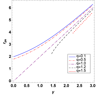
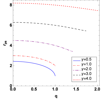
Figure 1: Change of the photon sphere radius $r_{ps}$ with parameters $q$ and $\gamma$ in the background of a black hole spacetime with torsion (II). Here, we set $m=1$.

As expected, the radius of the photon sphere $r_{ps}$ depends on both the parameters $q$ and $\gamma$ of the black hole. However, the appearance of $\gamma$ yields that the form of the photon sphere radius become very complicated in this case. In Fig.1, we present the variety of the photon sphere $r_{ps}$ with the parameter $q$ and $\gamma$ of by solving Eq. (31) numerically. It is shown that the photon sphere radius increases with the parameter $\gamma$ and decreases with $q$. The change of $r_{ps}$ with $q$ is similar to that in the Reissner-Nordström spacetime.

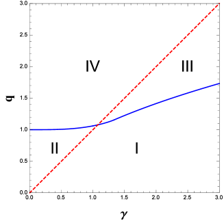
Figure 2: The boundary of the existence of horizon (red dashed line) and of the photon sphere (blue line) in the background of a black hole spacetime with torsion (II). Here, we set $m=1$.

Moreover, we find that the photon sphere $r_{ps}$ exists only in the regime $q<q_{c}$. The value of the upper limit $q_{c}$ depends on the parameter $\gamma$, and its form can be expressed as

$$q_{c}=\left\{\begin{array}[]{lll}\frac{m}{2\sqrt{6}}\bigg{[}\frac{\mathcal{W}^{2/3}+2(9\gamma^{2}+4)\mathcal{W}^{1/3}+(9\gamma^{2}-8)^{2}}{\mathcal{W}^{1/3}}\bigg{]}^{1/2},&&0<\gamma\leq 1,\\ \\ \frac{m}{4\sqrt{3}}\bigg{[}\frac{(-1-\sqrt{3}i)\mathcal{W}^{2/3}+4(9\gamma^{2}+4)\mathcal{W}^{1/3}+(-1+\sqrt{3}i)(81\gamma^{4}+64)^{2}}{\mathcal{W}^{1/3}}\bigg{]}^{1/2},&&1\leq\gamma\leq\frac{4}{3},\\ \\ \sqrt{\gamma},&&\gamma\geq\frac{4}{3},\end{array}\right.$$ (37)

where

$$\mathcal{W}=54\gamma^{2}\sqrt{2(27\gamma^{3}-18\gamma-8)(3\gamma-4)^{3}}|\gamma-1|+2187\gamma^{6}-5832\gamma^{5}+4860\gamma^{4}-1728\gamma^{2}+512.$$ (38)

Comparing Eq. (19) with Eq. (37), one can find that the condition of existence of horizons is not inconsistent with that of the photon sphere, which is also shown in Fig.(2). The red dashed line is the boundary for existence of horizon and the blue solid line is for photon sphere. It is obvious that the whole region in the parameter panel $(\gamma,q)$ is split into four regions $I$-$IV$ by those critical curves. When the parameters $(\gamma,q)$ lie in the region $I$, there exist both horizon and photon sphere radius $r_{ps}$, which is similar to that of in the static black hole spacetime in the Einstein’s general relativity. When $(\gamma,q)$ lie in the region $IV$, there is neither horizon nor photon sphere, which corresponds to case of strong naked singularity where the singularity is completely naked KS4 ; Gyulchev1 . When $(\gamma,q)$ is located in region $II$, there exists only photon sphere but no horizon, which corresponds to case of weak naked singularity where the singularity is covered by the photon sphere KS4 ; Gyulchev1 . When $(\gamma,q)$ lies in the region $III$, there is horizon but no photon sphere. These four situations are similar to those in the black hole spacetime with a torsion zchen . The special situation in which the black hole owns horizon but no photon sphere is absent in other theories of gravity. Thus, the presence of torsion changes the spacetime structure which will affect the propagation of photon in the background spacetime.

Let us now to discuss the behavior of the deflection angle of light ray in the spacetime described by a metric with torsion (II). For the photon coming from infinity, the deflection angle in a curved spacetime can be expressed as

$$\alpha(r_{0})=I(r_{0})-\pi,$$ (39)

where $r_{0}$ is the closest approach distance and $I(r_{0})$ is KS1

$$I(r_{0})=2\int^{\infty}_{r_{0}}\frac{\sqrt{\mathcal{B}(r)}dr}{\sqrt{C(r)}\sqrt{\frac{C(r)\mathcal{A}(r_{0})}{C(r_{0})\mathcal{A}(r)}-1}}.$$ (40)

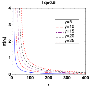
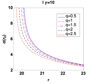
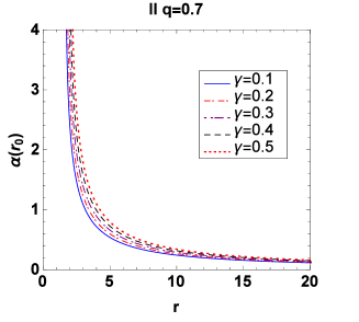
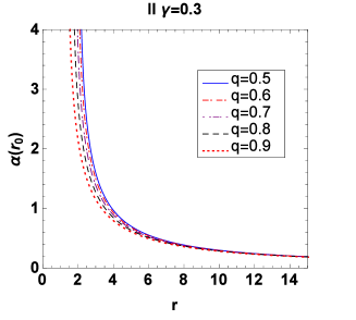
Figure 3: Deflection angle $\alpha(r_{0})$ as a function of the closest distance of approach $r_{0}$ for the cases with photon sphere. The panels in the upper and bottom rows correspond to the cases in which the parameters ($\gamma,q$) are located in the regions $I$ and $II$ in Fig.(2), respectively. Here, we set $m=1$.

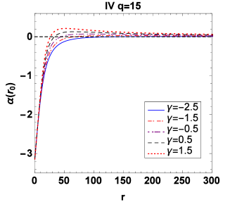
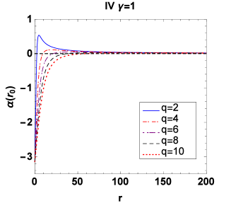
Figure 4: Deflection angle $\alpha(r_{0})$ as a function of the closest distance of approach $r_{0}$ for the case without photon sphere and horizon in which the parameters ($\gamma,q$) lie in the region $IV$ in Fig.(2). Here, we set $m=1$.

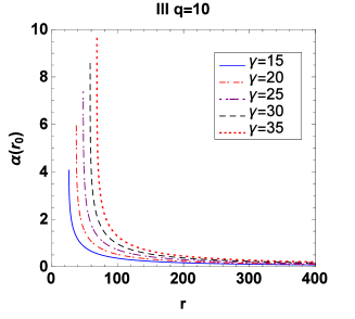
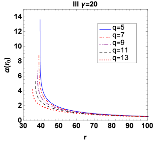
Figure 5: Deflection angle $\alpha(r_{0})$ as a function of the closest distance of approach $r_{0}$ for the case with horizon and no photon sphere in which the parameters ($\gamma,q$) lie in the region $III$ in Fig.(2). Here, we set $m=1$.

In Figs.(3)-(5), we plot the change of the deflection angle $\alpha(r_{0})$ with the distance of approach $r_{0}$ for different parameters $\gamma$ and $q$ in the spacetime with torsion (II). For the cases with photon sphere, i.e., the parameters ($\gamma,q$) lie in the region $I$ or $II$ in Fig.(2), the deflection angle for different $\gamma$ and $q$ strictly increases with the decreases of the closest distance of approach $r_{0}$ and finally becomes infinite as $r_{0}$ tends to the respective photon sphere radius $r_{ps}$, i.e., $\text{lim}_{r_{0}\rightarrow r_{ps}}\alpha(r_{0})=\infty$, which is shown in Fig.(3). In Fig.(4), we present the deflection angle in the case in which the parameters ($\gamma,q$) lie in the region $IV$ in Fig.(2). There is neither horizon nor photon sphere so that the singularity is naked completely. It is shown that the deflection angle of the light ray closing to the naked singularity tends to a finite value $-\pi$ for different $\gamma$ and $q$, which means that the photon could not be captured by the compact object so that the photon goes back along the original direction in this situation. This behavior can be regarded as a common feature of gravitational lensing by strong naked singularity. As the parameters ($\gamma,q$) lie in the region $III$ in Fig.(2), there exists horizon but no photon sphere, we find that the deflection angle of the light finally becomes a finite value as $r_{0}$ tends to the respective event horizon radius $r_{H}$, i.e., $\text{lim}_{r_{0}\rightarrow r_{H}}\alpha(r_{0})=\alpha_{r_{H}}$. This behavior differs from those in the black hole with a torsion considered in Ref.zchen in which the deflection angle of the light finally becomes unlimited large as $r_{0}$ tends to the event horizon radius. It could be understand by a fact that due to nonexistence of photon sphere the photon is captured directly by black hole before it make infinite complete loops around the central object in this case. Moreover, we find that the deflection angle $\alpha_{r_{H}}$ increases with the parameter $\gamma$ and decreases with $q$. In the far-field limit, the deflection angle can be approximated as

$$\alpha|_{r_{0}\rightarrow\infty}\simeq\frac{2(\gamma+1)m}{r_{0}}+\frac{(6\pi-8)(\gamma+1)m^{2}+3\pi(\gamma^{2}m^{2}-q^{2})}{4r^{2}_{0}},$$ (41)

which means that $\text{lim}_{r_{0}\rightarrow\infty}\alpha(r_{0})=0$ for all values of parameters $\gamma$ and $q$, which is a common feature in all asymptotical flat spacetimes.

We are now in position to study the strong gravitational lensing by a compact object (II) with the photon sphere and then probe how the parameters $\gamma$ and $q$ affect the coefficients in the strong field limit. Using of the method developed by Bozza VB1 , one can define a variable

$$z=1-\frac{r_{0}}{r},$$ (42)

and then rewrite the integral (40) as

$$I(r_{0})=\int^{1}_{0}R(z,r_{0})f(z,r_{0})dz,$$ (43)

with

$$R(z,r_{0}) = 2\sqrt{\mathcal{A}(r)\mathcal{B}(r)C(r)},$$ (44)

$$f(z,r_{0}) = \frac{1}{\sqrt{\mathcal{A}(r_{0})C(r)-\mathcal{A}(r)C(r_{0})}}.$$ (45)

The function $R(z,r_{0})$ is regular for all values of $z$ and $r_{0}$, but $f(z,r_{0})$ diverges as $z$ tends to zero. Thus, one can split the integral (43) into the divergent part $I_{D_{1}}(r_{0})$ and the regular part $I_{R}(r_{0})$,

$$I_{D}(r_{0}) = \int^{1}_{0}R(0,r_{ps})f_{0}(z,r_{0})dz,$$

$$I_{R}(r_{0}) = \int^{1}_{0}[R(z,r_{0})f(z,r_{0})-R(0,r_{ps})f_{0}(z,r_{0})]dz.$$ (46)

Expanding the argument of the square root in $f(z,r_{0})$ to the second order in $z$, one can obtain

$$f_{0}(z,r_{0})=\frac{1}{\sqrt{\alpha(r_{0})z+\beta(r_{0})z^{2}}},$$ (47)

with

$$\alpha(r_{0}) = \frac{2}{(\gamma^{2}-q^{2})^{2}\sqrt{r^{2}_{0}-2\gamma r_{0}+q^{2}}}\bigg{[}(\gamma-1)(q^{2}-\gamma r_{0})+(q^{2}-\gamma)\sqrt{r^{2}_{0}-2\gamma r_{0}+q^{2}}\bigg{]}$$

$$\times \bigg{[}(\gamma-q^{2})(r^{2}_{0}-3\gamma r_{0}+2q^{2})+(\gamma-1)(\gamma r_{0}-2q^{2})\sqrt{r^{2}_{0}-2\gamma r_{0}+q^{2}}\bigg{]},$$

$$\beta(r_{0}) = \frac{1}{(\gamma^{2}-q^{2})^{2}}\bigg{\{}(\gamma-1)(q^{2}-\gamma)\bigg{[}\frac{r_{0}(\gamma r_{0}-q^{2})[2r_{0}^{3}-6\gamma r_{0}^{2}-2\gamma q^{2}+3(\gamma^{2}+q^{2})r_{0}]}{(r^{2}_{0}-2\gamma r_{0}+q^{2})^{3/2}}$$ (48)

$$+ \frac{2r_{0}(\gamma-r_{0})(\gamma r_{0}-2q^{2})}{\sqrt{r^{2}_{0}-2\gamma r_{0}+q^{2}}}-2(3\gamma r_{0}-2q^{2})\sqrt{r^{2}_{0}-2\gamma r_{0}+q^{2}}\bigg{]}+2q^{6}-6\gamma^{3}r_{0}$$

$$+ [3r_{0}^{2}-6\gamma r_{0}+2(\gamma^{2}-4\gamma+1)]q^{4}-2\gamma[3r_{0}^{2}+3(\gamma^{2}-4\gamma+1)r_{0}-\gamma]q^{2}+3\gamma^{2}r_{0}^{2}(\gamma^{2}-2\gamma+2)\bigg{\}}.$$

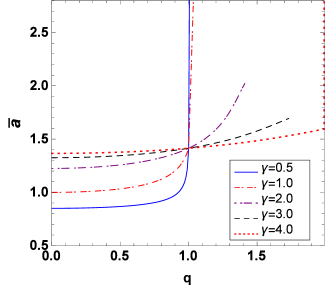
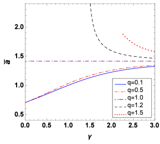
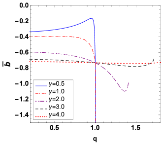
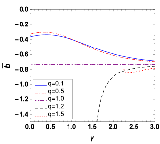
Figure 6: Change of the strong deflection limit coefficients $\bar{a}$ and $\bar{b}$ with the parameters $\gamma$ and $q$ in the spacetime with torsion (II).

It is obvious that the coefficient $\alpha(r_{0})$ vanishes as $r_{0}$ tends to the radius of photon sphere $r_{ps}$, and then the leading term of the divergence in $f_{0}(z,r_{0})$ is $z^{-1}$. This means that near the photon sphere the deflection angle of light ray can be expressed as VB1

$$\alpha(\theta)=-\bar{a}\ln{\bigg{(}\frac{\theta D_{OL}}{u_{ps}}-1\bigg{)}}+\bar{b}+O(u-u_{ps}),$$ (49)

with

$$\bar{a} =\frac{R(0,r_{ps})}{2\sqrt{\beta(r_{ps})}},$$ (50)

$$\bar{b} =-\pi+b_{R}+\bar{a}\ln{\frac{r^{2}_{ps}[C^{\prime\prime}(r_{ps})\mathcal{A}(r_{ps})-C(r_{ps})\mathcal{A}^{\prime\prime}(r_{ps})]}{u_{ps}\sqrt{\mathcal{A}^{3}(r_{ps})C(r_{ps})}}},$$

$$b_{R} =I_{R}(r_{ps}),\;\;\;\;\;u_{ps}=\frac{r_{ps}}{\sqrt{\mathcal{A}(r_{ps})}},$$

which indicates clearly that the deflection angle diverges logarithmically where the light is close to the photon sphere. The quantity $D_{OL}$ is the distance between gravitational lens object and observer, $\bar{a}$ and $\bar{b}$ are the strong field limit coefficients which depend on the spacetime functions at the photon sphere. The changes of the coefficients ($\bar{a}$ and $\bar{b}$ ) with the parameters $\gamma$ and $q$ is shown in Fig.(6). For the fixed $\gamma$, the coefficient $\bar{a}$ increases monotonously with $q$. With increase of $q$, the coefficient $\bar{b}$ first increases and then decreases for the smaller $\gamma$, but first decreases and then increases for the larger $\gamma$. With increase of the parameter $\gamma$, $\bar{a}$ increases monotonously as $q<1$ and decreases as $q>1$, $\bar{b}$ first increases and then decreases as $q<1$. For the case with $q>1$, $\bar{b}$ increases with $\gamma$ as the quantity $q-1$ is small. With the further increase of $q$, the change of $\bar{b}$ shows gradually a tendency of first decreasing and then increasing.

Let us now to estimate the numerical values for the observables of gravitational lensing in the strong field limit by assuming that the spacetime of the supermassive compact object at the Galactic center of Milky Way can be described by the metric (II).

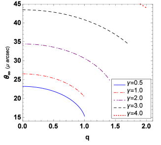
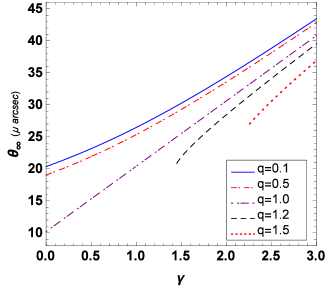
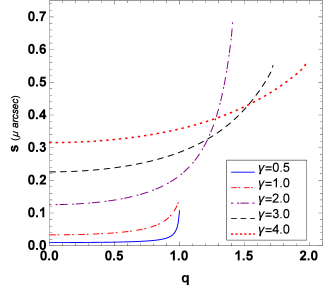
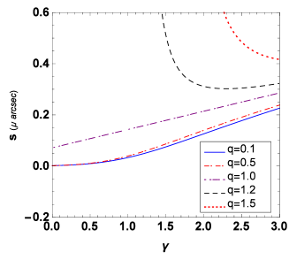
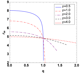
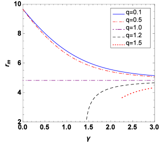
Figure 7: Gravitational lensing by the center black hole in Milk Way Galaxy. Variation of the values of the angular position $\theta_{\infty}$, the angular separation $s$, and the relative magnitudes $r_{m}$ with the parameters $q$ and $\gamma$ in the spacetime with torsion (II).

As the light source and observer are far enough from the central compact object, the corresponding lens equation can be expressed as VB2

$$\bar{\gamma}=\frac{D_{OL}+D_{LS}}{D_{LS}}\theta-\alpha(\theta)\;mod\;2\pi$$ (51)

where $D_{LS}$ is the lens-source distance and $D_{OL}$ is the observer-lens distance. $\bar{\gamma}$ is the angle between the optical axis and the direction of the source. $\theta$ is the angular separation between the lens and the image, which has a form $\theta=u/D_{OL}$. As in Ref.VB2 , we here focus only on the simplest situation in which the source, lens and observer are highly aligned so that the angular separation between the lens and the $n$-th relativistic image can be simplified as

$$\theta_{n}\simeq\theta^{0}_{n}\bigg{(}1-\frac{u_{ps}e_{n}(D_{OL}+D_{LS})}{\bar{a}D_{OL}D_{LS}}\bigg{)},$$ (52)

with

$$\theta^{0}_{n}=\frac{u_{ps}}{D_{OL}}(1+e_{n}),\;\;\;\;\;\;e_{n}=e^{\frac{\bar{b}+|\bar{\gamma}|-2\pi n}{\bar{a}}},$$ (53)

where $\theta^{0}_{n}$ is the image positions corresponding to $\alpha=2n\pi$, and $n$ is an integer. As $n\rightarrow\infty$, from Eqs.(52) and (53), it is easy to find that $e_{n}$ tends to zero, which means that the relationship between the asymptotic position of a set of images $\theta_{\infty}$ and the minimum impact parameter $u_{ps}$ owns a simpler form

$$u_{ps}=D_{OL}\theta_{\infty}.$$ (54)

In order to estimate the coefficients $\bar{a}$ and $\bar{b}$ as in Refs.VB1 ; VB2 , we can consider a perfect situation in which only the outermost image $\theta_{1}$ is separated as a single image and all the remaining ones are packed together at $\theta_{\infty}$. And then, the angular separation $s$ and the relative magnitudes $r_{m}$ between the first image and other ones can be simplified further as VB1 ; VB2 ; Gyulchev1

$$s = \theta_{1}-\theta_{\infty}=\theta_{\infty}e^{\frac{\bar{b}-2\pi}{\bar{a}}},$$

$$r_{m} = 2.5\log{\frac{\mu_{1}}{\sum^{\infty}_{n=2}\mu_{n}}}=\frac{5\pi}{\bar{a}}\log{e},$$ (55)

Therefore, one can obtain the coefficients $\bar{a}$, $\bar{b}$ in strong deflection limit and the minimum impact parameter $u_{ps}$ through measuring $s$, $\theta_{\infty}$ and $r_{m}$ from observation experiments and extract further information about the central compact object. For Milk Way Galaxy, the mass of the central object of is estimated recently to be $4.4\times 10^{6}M_{\odot}$ Genzel1 and its distance is around $8.5kpc$, which leads to the ratio of the mass to the distance $M/D_{OL}\approx 2.4734\times 10^{-11}$. With these data, we present the numerical value for the angular position of the relativistic images $\theta_{\infty}$, the angular separation $s$ and the relative magnitudes $r_{m}$ in Fig.(7). It is shown that the angular position of the relativistic images $\theta_{\infty}$ decreases with the parameter $q$ and increases with the parameter $\gamma$. The angular separation $s$ between $\theta_{1}$ and $\theta_{\infty}$ increases with the tidal-like charge $q$. With increase of $\gamma$, $s$ increases for the smaller $q$ case and decreases for the larger $q$ case. The change of $r_{m}$ with the parameters $q$ and $\gamma$ is converse to that of the angular separation $s$.

Finally, we make a brief comparison among the main features of strong gravitational lensing by compact objects in different gravitational theories, which is shown in Table (I). It tells us that the event horizon and photon sphere are two important surfaces in the propagation of light rays. From Table (I), it is obvious that in the cases with photon sphere the deflection angle $\alpha$ for the light ray near the photon sphere diverges logarithmically, which can be regarded as a common feature in the strong gravitational lensing by compact objects in various theories of gravity. In the cases of strong naked singularity where there is neither photon sphere nor horizon, the deflection angle $\alpha$ for the light ray near singularity tends to a finite value $\alpha_{s}$. The sign and value of $\alpha_{s}$ depend on the spacetime parameters.

	Existence		Deflection angle $\alpha$ close to
Spacetimes	Event	Photon	Event	Photon		Literature
	horizon	sphere	horizon	sphere	Singularity
Schwarzschild black hole	yes	yes	-	$\infty$	-	VB1 ; KS2
Reissner-Nördström black hole	yes	yes	-	$\infty$	-	VB1 ; Eirc1
Kerr black hole	yes	yes	-	$\infty$	-	VB2 ; VB202
Janis-Newman-Winicour naked singularities	no	yes	-	$\infty$	-	KS4 ; Gyulchev1
	no	no	-	-	finite value
Dilaton black holes	yes	yes	-	$\infty$	-	Gyulchev ; Bhad1 ; TSa1
Hořava-Lifshitz black holes	yes	yes	-	$\infty$	-	Song1 ; Song1add
Squashed Kaluza-Klein black holes	yes	yes	-	$\infty$	-	Song101 ; gr4 ; gr401
Braneworld black holes	yes	yes	-	$\infty$	-	whisk ; AnAv ; bran1
Eddington-inspired Born-Infeld black holes	yes	yes	-	$\infty$	-	agl1 ; agl1add
Einstein-Born-Infeld black holes	yes	yes	-	$\infty$	-	agl1add0
Black Holes in Loop Quantum Gravity	yes	yes	-	$\infty$	-	agl101
Black hole pierced by a cosmic string	yes	yes	-	$\infty$	-	gr201
Kerr-Taub-NUT spacetime	yes	yes	-	$\infty$	-	gr2
Gauss-Bonnet black hole	yes	yes	-	$\infty$	-	gr51
Johannsen-Psaltis rotating non-Kerr spacetime	yes	yes	-	$\infty$	-	Song102
	no	no	-	-	finite value
Konoplya-Zhidenko rotating non-Kerr spacetime	yes	yes	-	$\infty$	-	Song2
	no	yes	-	$\infty$	-
	no	no	-	-	finite value
Phantom black holes	yes	yes	-	$\infty$	-	gr1 ; gr1add0 ; gr1add
Noncommutative black hole	yes	yes	-	$\infty$	-	gr1noncom
Einstein-Skyrme black hole	yes	yes	-	$\infty$	-	glcom31
Horndeski black hole	yes	yes	-	$\infty$	-	glcom32 ; glcom33
Black hole in massive gravity	yes	yes	-	$\infty$	-	mg1
Black hole in Chern-Simons modified gravity	yes	yes	-	$\infty$	-	CSmg
Black hole in F(R) gravity	yes	yes	-	$\infty$	-	fR1 ; fR2
Wormholes	no	yes	-	$\infty$	-	worm1 ; worm2 ; worm3
High dimensional black holes	no	yes	-	$\infty$	-	Exdim1 ; Exdim2
Charged black holes in scalar-tensor gravity	no	yes	-	$\infty$	-	Scatensor
Bardeen spacetime	yes	yes	-	$\infty$	-	Bardeen
	no	yes	-	$\infty$	-
	no	no	-	-	finite value
Spacetime with torsion sbh1 in ECKS theory	yes	yes	-	$\infty$	-	zchen
	no	yes	-	$\infty$	-
	yes	no	$\infty$	-	-
	no	no	-	-	finite value
Spacetime with torsion (II) in ECKS theory	yes	yes	-	$\infty$	-	In our current work
	no	yes	-	$\infty$	-
	yes	no	finite value	-	-
	no	no	-	-	finite value

Table 1: Comparison among the main features of gravitational lensing by compact objects in different gravitational theories.

From Table.(I), we also note that only in the spacetimes with a torsion in generalized ECKS theory considered here or in Ref.zchen , there is a special parameter region in which there exists only horizon but no photon sphere. In this special parameter region, the deflection angle $\alpha$ is also logarithmically divergent as the light ray approaches the event horizon in the spacetime sbh1 . However, for the spacetime (II), we find that the deflection angle $\alpha$ tends to a certain finite value as the light ray approaches the event horizon, which could be understand by a fact that the photon is captured directly by black hole before it make infinite complete loops around the central object. For the black holes in general relativity (i.e., the coupling coefficient $a_{1}=0$ ), such as, Schwarzschild and Kerr black holes, one can find that the photon sphere lies always outside of the event horizon and then for the light ray from infinity the deflection angle $\alpha$ diverges logarithmically as the closest approach distance $r_{0}$ tends to the photon sphere, which means that photons are captured by black hole once they reach the photon sphere. However, in the generalized ECKS theory, there are a special kind of black hole without photon sphere (II) or in Ref.sbh1 , so that photons can be captured by black hole only when they reach the event horizon, which differs from that in the black holes in general relativity and other theories of gravity. Moreover, comparing with in Reissner-Nördström black hole case, as $\gamma>1$, due to the larger coefficient $\bar{a}$, the deflection angle for light ray with the same $r_{0}$ in the strong field limit is larger in the spacetime of the black hole with photon sphere (II). Similarly, the observables $\theta_{\infty}$ and $s$ have larger values. However, as $\gamma<1$, the deflection angle, the observables $\theta_{\infty}$ and $s$ are less than that in Reissner-Nördström black hole case. On the contrary, comparing with in Reissner-Nördström black hole spacetime, the relative magnitudes $r_{m}$ is smaller for the cases with $\gamma>1$ and is larger for the cases with $\gamma<1$. These deviation from the cases in general relativity could help us in understanding the gravitational lensing caused by torsion in the generalized ECKS theory of gravity.

IV summary

In this paper we firstly present a new black hole solution in the generalized ECKS gravity with three independent parameters $m$, $q$ and $\gamma$ and then investigate the propagation of photon in this background. We find that these spacetime parameters affect sharply photon sphere, deflection angle of light ray and strong gravitational lensing. The photon sphere exists only in the regime $q<q_{c}$ and the value of $q_{c}$ depends on the parameter $\gamma$. In the regime where photon sphere exists, the radius of photon sphere increases with the parameter $\gamma$, but decreases with $q$. Moreover, the condition of existence of horizons is not inconsistent with that of photon sphere, which yields that the whole region in the panel ($\gamma,q$) can be split into four regions by the boundaries of the existence of horizon and of the photon sphere. In the cases with photon sphere, the deflection angle of the light ray near the photon sphere diverges logarithmically, which is similar to those in the usual spacetime of a black hole or a weak naked singularity in the strong-field limit. In the case without photon sphere and horizon, the deflection angle of the light ray closing very to the singularity approaches a finite value $-\pi$, which does not depend on spacetime parameters $\gamma$ and $q$. It should be a common feature of the deflection angle of light ray near the static strong naked singularity. Furthermore, we also find that there exists a special case in which there is horizon but no photon sphere for the spacetime (II) as in the spacetime with a torsion zchen . However, we find that the deflection angle of the light ray near the event horizon tends to a finite value in this case, which differs from those in the black hole with a torsion considered in Ref.zchen where the deflection angle of the light finally becomes diverges logarithmically. It could be attribute to that the photon is captured directly by black hole before it make infinite complete loops around the central object in this case. Finally, we studied the strong gravitational lensing by a compact object (II) with the photon sphere and then probed how the parameters $\gamma$ and $q$ affect the coefficients in the strong field limit.

V Acknowledgments

We would like to thank the referee for useful comments. This work was partially supported by the National Natural Science Foundation of China under Grant No. 11875026, the Scientific Research Fund of Hunan Provincial Education Department Grant No. 17A124. J. Jing’s work was partially supported by the National Natural Science Foundation of China under Grant No. 11475061, 11875025.

References

- (1) A. G. Riess et al., Astron. J. 116 1009 (1998).
- (2) A. G. Riess et al., Astrophys. J. 659 98 (2007).
- (3) P. de Bernardis et al., Nature (London) 404 955 (2000).
- (4) S. Perlmutter et al., Astrophys. J. 517 565 (1999).
- (5) R. A. Knop et al., Astrophys. J. 598 102 (2003).
- (6) E. Cartan, C. R. Acad. Sci. (Paris) 174, 593 (1922); E. Cartan, Ann. Ec. Norm. Sup. 40, 325 (1923); E. Cartan, Ann. Ec. Norm. Sup. 41, 1 (1924); E. Cartan, Ann. Ec. Norm. Sup. 42, 17 (1925).
- (7) T. W. B. Kibble, J. Math. Phys. 2, 212 (1961); D. W. Sciama, Rev. Mod. Phys. 36, 463 (1964); F. Hehl and E. Kroner, Z. Phys. 187, 478 (1965); F. Hehl, Abb. Braunschweig. Wiss. Ges. 18, 98 (1966); F. Hehl, P. Heyde, G. Kerlick, J. Nester, Rev. Mod. Phys. 48, 393 (1976). A. Trautman, Bull. Polon. Acad. Sci. 20, 185 (1972); A. Trautman, Bull. Polon. Acad. Sci. 20, 503 (1972).
- (8) W. Kopczyński, Phys. Lett. A 39, 219 (1972); Phys. Lett. A 43, 63 (1973).
- (9) A. Trautman, Nature (Phys. Sci.) 242, 7 (1973); J. Tafel, Phys. Lett. A 45, 341 (1973); F. Hehl, P. von der Heyde, and G. Kerlick, Phys. Rev. D 10, 1066 (1974); B. Kuchowicz, Gen. Relativ. Gravit. 9, 511 (1978); M. Gasperini, Phys. Rev. Lett. 56, 2873 (1986); M. Gasperini, Gen. Relativ. Gravit. 30, 1703 (1998).
- (10) N. Poplawski, Phys. Rev. D, 85 107502 (2012); Gen. Relativ. and Gravit., 44 1007 (2012); Phys. Lett. B, 690 73 (2010).
- (11) S. D. Brechet, M. P. Hobson, A. N. Lasenby, Class. Quantum Grav. 25 245016 (2008).
- (12) Y. N. Obukhov, V. N. Ponomarev and V. V. Zhytnikov, Gen. Rel. Grav. 21 1107 (1989); Y. N. Obukhov, Int. J. Geom. Meth. Mod. Phys. 3 95 (2006).
- (13) S. M. Christensen, J. Phys. A: Math. Gen. 13 3001 (1980).
- (14) E. Sezgin, P. V. Nieuwenhuizen, Phys. Rev. D, 21 3269 (1980).
- (15) M. Leclerc, Int. J. Mod. Phys. D 16, 655 (2007).
- (16) J. A. R. Cembranos and J. G. Valcarcel,J. Cosmol. Astropart. Phys. 01, 014 (2017), arXiv:1608.00062 [gr-qc].
- (17) H. Shabani, and A. Hadi Ziaie, Int. J. Mod. Phys. A 33, 1850095 (2018), arXiv:1709.06512.
- (18) K. Hayashi and T. Shirafuji, Phys. Rev. D 19, 3524 (1979) [Phys. Rev. D 24, 3312 (1982)].
- (19) R. Casadio, A. Fabbri, L. Mazzacurati, Phys. Rev. D 65, 084040 (2002).
- (20) A. Einstein, Science 84 506 (1936).
- (21) C. Darwin, Proc. R. Soc. London 249 180 (1959).
- (22) K. S. Virbhadra, D. Narasimha, and S. M. Chitre, Astron. Astrophys. 337 1 (1998).
- (23) K. S. Virbhadra and G. F. R. Ellis, Phys. Rev. D 62 084003 (2000); C. M. Claudel, K. S. Virbhadra, and G. F. R. Ellis, J. Math. Phys. (N.Y.) 42 818 (2001).
- (24) K. S. Virbhadra and G. F. R. Ellis, Phys. Rev. D 65 103004 (2002).
- (25) V. Bozza, Phys. Rev. D 66 103001 (2002).
- (26) V. Bozza, Phys. Rev. D 67 103006 (2003); V. Bozza, F. De Luca, G. Scarpetta, and M. Sereno, Phys. Rev. D 72 083003 (2005).
- (27) V. Bozza, F. De Luca, and G. Scarpetta, Phys. Rev. D 74 063001(2006).
- (28) G. N. Gyulchev and S. S. Yazadjiev, Phys. Rev. D 75 023006 (2007).
- (29) G. N. Gyulchev and S. S. Yazadjiev, Phys. Rev. D 78 083004 (2008).
- (30) S. Frittelly, T. P. Kling, E. T. Newman, Phys. Rev. D 61 064021 (2000).
- (31) V. Bozza, S. Capozziello, G. lovane, G. Scarpetta, Gen. Rel. and Grav. 33 1535 (2001).
- (32) E. F. Eiroa, G. E. Romero, D. F. Torres, Phys. Rev. D 66 024010 (2002).
- (33) R. Whisker, Phys. Rev. D 71 064004 (2005).
- (34) A. Bhadra, Phys. Rev. D 67 103009 (2003).
- (35) S. Chen and J. Jing, Phys. Rev. D 80 024036 (2009).
- (36) Z. Horváth, L. Gergely, Z. Keresztes, T. Harko, F. Lobo, Phys. Rev. D 84, 083006 (2011).
- (37) Y. Liu, S. Chen and J. Jing, Phys. Rev. D 81 124017 (2010); S. Chen, Y. Liu and J. Jing, Phys. Rev. D 83 124019 (2011); L. Ji, S. Chen, J. Jing, J. High Energ. Phys. 1403, 089 (2014).
- (38) S. Chen and J. Jing, Phys. Rev. D 85 124029 (2012).
- (39) S. Chen, S. Wang, Y. Huang, J. Jing, S. Wang, Phys. Rev. D 95, 104017 (2017); S. Chen, J. Jing, J. Cosmol. Astropart. Phys. 10, 002 (2015).
- (40) S. Wang, S. Chen, J. Jing, J. Cosmol. Astropart. Phys. 11, 020 (2016).
- (41) T. Ghosh, S. Sengupta, Phys. Rev. D 81 044013 (2010).
- (42) A. N. Aliev, P. Talazan, Phys. Rev. D 80 044023 (2009).
- (43) E. F. Eiroa, C. M. Sendra, Phys. Rev. D 86, 083009 (2012).
- (44) H. Sotani and U. Miyamoto, Phys. Rev. D 92 044052 (2015).
- (45) Shao-Wen Wei, Ke Yang, Yu-Xiao Liu, Eur. Phys. J. C 75 253 (2015).
- (46) E. F. Eiroa, Phys. Rev. D 73, 043002 (2006).
- (47) S. Sahu, K. Lochan and D. Narasimha, Phys. Rev. D 91, 063001 (2015).
- (48) C. Ding, C. Liu, Y. Xiao, L. Jiang and R. Cai, Phys. Rev. D 88, 104007 (2013).
- (49) E. F. Eiroa and C. M. Sendra, Phys. Rev. D 88 103007 (2013).
- (50) G. N. Gyulchev, I. Z. Stefanov, Phys. Rev. D87, 063005 (2013)
- (51) C. Ding, S. Kang, C. Chen, S. Chen, J. Jing, Phys. Rev. D 83,084005 (2011).
- (52) S. Wei, Y. Liu, C. Fu and K. Yang, J. Cosmol. Astropart. Phys. 1210 053 (2012).
- (53) S. Wei, Y. Liu, Phys. Rev. D 85 064044 (2012).
- (54) G. V. Kraniotis, Class. Quant. Grav. 28 085021 (2011).
- (55) J. Sadeghi, H. Vaez, Phys. Lett. B 728 170 (2014).
- (56) J. Sadeghi, A. Banijamali and H. Vaez, Astrophys. Space Sci. 343 559 (2013).
- (57) J. Sadeghi, H. Vaez, J. Cosmol. Astropart. Phys. 1406, 028 (2014).
- (58) F. Canfora, E. F. Eiroa, C. M. Sendra, arXiv:1805.03626.
- (59) J. Badia, E. F. Eiroa, Eur. Phys. J. C 77, 779 (2017).
- (60) S. Zhao, Y. Xie, J. Cosmol. Astropart. Phys.1607 007, (2016).
- (61) R. Zhang, J. Jing, S. Chen, Phys. Rev. D 95, 064054 (2017).
- (62) S. Chen, J. Jing, Class. Quant Grav.27, 225006 (2010).
- (63) J. Man, H. Cheng, Phys. Rev. D 92, 024004 (2015).
- (64) A. Nzioki, P. Dunsby, R. Goswami, S. Carloni, Phys. Rev. D 83, 024030 (2011).
- (65) K. Jusufi, A. Övgün, Phys. Rev. D 97, 024042 (2018).
- (66) R. Shaikh, S. Kar, Phys. Rev. D 96, 044037 (2017).
- (67) N. Tsukamoto, Phys. Rev. D 94, 124001 (2016).
- (68) S. Chakraborty, S. SenGupta, J. Cosmol. Astropart. Phys. 1707, 045 (2017).
- (69) N. Tsukamoto, T. Kitamura, K. Nakajima, H. Asada, Phys. Rev. D 90,064043 (2014).
- (70) E. F. Eiroa, C. M. Sendra, Eur. Phys. J. C 74, 3171 (2014).
- (71) J. Schee, Z. Stuchlik, J. Cosmol. Astropart. Phys. 1506, 048 (2015).
- (72) L. Zhang, S. Chen, J. Jing, Int. J. Mod. Phys. D 27, 1850110 (2018); arXiv:1712.00160.
- (73) Y. M. Cho, Phys. Rev. D 14, 2521 (1976).
- (74) F. W. Hehl, Y. Neéman, J. Nitsch and P. Von der Heyde, Phys. Lett. B 78, 102 (1978).
- (75) J. Nitsch and F. W. Hehl, Phys. Lett. B 90, 98 (1980).
- (76) J. W. Maluf and F. F. Faria, Phys. Rev. D 85, 027502 (2012).
- (77) C. Q. Geng and L. W. Luo, Class. Quant. Grav. 34, 115012 (2017).
- (78) M. Tsamparlis, Phys. Lett. A 75, 27 (1979); Phys. Rev. D 24, 1451 (1981).
- (79) R. Shaikh, S. Kar, Phys. Rev. D 94, 024011 (2016).
- (80) F. W. Hehl, P. von der Heyde and G.D. Kerlick, Rev. Mod. Phys. 48, 393 (1976); F. W. Hehl and Y.N. Obukhov, Annales Fond. Broglie 32, 157 (2007).
- (81) K. Pasmatsiou, C. G. Tsagas, J. D. Barrow, Phys. Rev. D 95, 104007 (2017)
- (82) R. Genzel, F. Eisenhauer and S. Gillessen, Rev. Mod. Phys. 82 (2010) 3121, arXiv:1006.0064.