Sublattice Coding Algorithm and Distributed Memory Parallelization for Large-Scale Exact Diagonalizations of Quantum Many-Body Systems

Abstract

We present algorithmic improvements for fast and memory-efficient use of discrete spatial symmetries in Exact Diagonalization computations of quantum many-body systems. These techniques allow us to work flexibly in the reduced basis of symmetry-adapted wave functions. Moreover, a parallelization scheme for the Hamiltonian-vector multiplication in the Lanczos procedure for distributed memory machines avoiding load balancing problems is proposed. We demonstrate that using these methods low-energy properties of systems of up to $50$ spin-$1/2$ particles can be successfully determined.

I Introduction

Exact Diagonalization, short ED, studies have in the past been a reliable source of numerical insight into various problems in quantum many-body physics, ranging from quantum chemistry Gan and Harrison (2005), nuclear structureSternberg et al. (2008); Vary et al. (2009); Maris et al. (2010), quantum field theory Rychkov and Vitale (2015) to strongly correlated lattice models in condensed matter physics. The method is versatile, unbiased and capable of simulating systems with a sign problem. The main limitation of ED is the typically exponential scaling of computational effort and memory requirements in the system size. Nevertheless, the number of particles or lattice sites feasible for simulation has steadily increased since the early beginnings Oitmaa and Betts (1978) and have provided valuable insight to many problems in modern condensed matter physics, for example, frustrated magnetism Wietek and Läuchli (2017); Wietek et al. (2015); Dagotto and Moreo (1989); Leung and Elser (1993); Schulz, H.J.  et al. (1996); Richter and Schulenburg (2010); Läuchli et al. (2012, 2016), high temperature superconductivity Lin and Hirsch (1987); Hasegawa and Poilblanc (1989); Bonča et al. (1989); Poilblanc (1995), quantum hall effect and fractional Chern insulators He et al. (1994); Morf et al. (2002); Neupert et al. (2011); Läuchli et al. (2013) and quantum critical points in 2+1 dimensions Schuler et al. (2016); Whitsitt et al. (2017). Different approaches for increasing the system size in these simulations have been proposed over time Lin (1990); Weiße (2013). Not only does increasing the number of particles yield better approximations to the thermodynamic limit, but also several interesting simulation clusters with many symmetries become available if more particles can be simulated. Having access to such clusters becomes important if several competing phases ought to be realized on the same finite size sample.

The ED method is essentially equivalent to simulating quantum circuits. With the advent of scalable experimental quantum computation Feynman (1982); Häffner et al. (2005); Castelvecchi (2017), exact classical simulation of quantum circuits has become important for benchmarking and validating results from actual quantum computers Häner and Steiger (2017); Pednault et al. (2017); Gheorghiu et al. (2017). At present, we are on the verge of quantum computers surpassing the capabilities of classical supercomputers in terms of the number of simulated Qubits, colloquially referred to as quantum advantage. Specifically, the barrier of classically simulating $50$ Qubits has not been breached to date.

In this work, we present algorithms and strategies for the implementation of a state-of-the-art large-scale ED code and prove that applying these methods systems of up to $50$ spin-$1/2$ particles can be simulated on present day supercomputers. There are two key ingredients making these computations possible:

• Efficient use of symmetries. We present an algorithm to work with symmetry-adapted wave functions in a fast and memory efficient way. This so-called sublattice coding algorithm allows us to diagonalize the Hamiltonian in every irreducible representation of a discrete symmetry group. The basic idea behind this algorithm goes back to H.Q. Lin Lin (1990). An extension of this method was proposed in Ref. Weiße (2013). We generalize these approaches to arbitrary discrete symmetries, varying number of sublattices and arbitrary geometries.

• Parallelization of the matrix-vector multiplications in the Lanczos algorithm Lanczos (1950) for distributed memory machines. We propose a method avoiding load-balancing problems in message-passing and present a computationally fast way of storing the Hilbert space basis.

These ideas have been implemented and tested on various supercomputers. We present results and benchmarks to demonstrate the efficiency and flexibility of the proposed methods.

II Symmetry adapted basis states

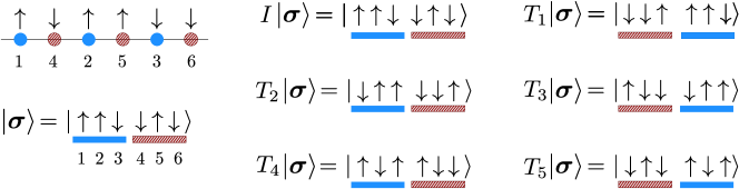
Figure 1: Two sublattice coding of the spin state $\ket{\bm{\sigma}}$ on a six-site chain lattice and action of translational symmetries. The sites are enumerated such that site $1$-$3$ are on the blue (solid) sublattice $A$, $4$-$6$ on the red (dashed) sublattice $B$. The representative state with this enumeration of sites is given by $\ket{\tilde{\bm{\sigma}}}=T_{1}\ket{\bm{\sigma}}=\ket{\downarrow\downarrow\uparrow\uparrow\uparrow\downarrow}$. Notice, that the symmetries act on real space and thus the transformation of the basis states also depends on the numbering of sites.

Employing symmetries in ED computations amounts to block diagonalizing the Hamiltonian. The blocks correspond to the irreducible representations of the symmetry group and the procedure of block diagonalization amounts to changing the basis of the Hilbert space to symmetry-adapted basis states. Here, we briefly review this basis and recall some basic notions commonly used in this context. For a more detailed introduction to this topic see e.g. Refs. Landau (1988); Läuchli (2011). In this manuscript, we only consider one-dimensional representations of the symmetry group. Consider a generic spin configuration on $N$ lattice sites with local dimension $d$,

$$\ket{\bm{\sigma}}=\ket{\sigma_{1},\ldots,\sigma_{N}},\quad\sigma_{i}\in\{1,\ldots,d\}.$$ (1)

The symmetry-adapted basis states $\ket{\bm{\sigma}_{\rho}}$ are given by

$$\ket{\bm{\sigma}_{\rho}}\equiv\frac{1}{N_{\rho,\bm{\sigma}}}\sum\limits_{g\in\mathcal{G}}\chi_{\rho}(g)^{*}{g}\ket{\bm{\sigma}},$$ (2)

where $\mathcal{G}$ denotes a discrete symmetry group, $\rho$ a one-dimensional representation of this group, $\chi_{\rho}(g)$ the character of this representation evaluated at group element $g$, and $N_{\rho,\bm{\sigma}}$ denotes the normalization constant of the state $\ket{\bm{\sigma}_{\rho}}$. The set of basis state spin configurations $\ket{\bm{\sigma}}$ is divided into orbits,

$$\text{Orbit}(\ket{\bm{\sigma}})=\{{g}\ket{\bm{\sigma}}|g\in\mathcal{G}\}.$$ (3)

We define,

$$\ket{\bm{\sigma}}<\ket{\bm{\sigma}^{\prime}}:\Leftrightarrow\operatorname{int}(\ket{\bm{\sigma}})<\operatorname{int}(\ket{\bm{\sigma}^{\prime}}),$$ (4)

where $\operatorname{int}(\ket{\bm{\sigma}})$ denotes an integer value coding on the computer for the spin configuration $\ket{\bm{\sigma}}$. The representative $\ket{\tilde{\bm{\sigma}}}$ within each orbit is given by the element with smallest integer value,

$$\ket{\tilde{\bm{\sigma}}}=g_{\bm{\sigma}}\ket{\bm{\sigma}},\quad g_{\bm{\sigma}}=\operatornamewithlimits{argmin}_{g\in\mathcal{G}}\,\text{int}(g\ket{\bm{\sigma}}).$$ (5)

The matrix element $\braket{\tilde{\bm{\sigma}^{\prime}}_{\rho}}{H_{k}}{\tilde{\bm{\sigma}}_{\rho}}$ for non-branching terms $H_{k}$ for two symmetry-adapted basis states with representation $\rho$ is given by

$$\braket{\tilde{\bm{\sigma}^{\prime}}_{\rho}}{H_{k}}{\tilde{\bm{\sigma}}_{\rho}}=\chi_{\rho}(g_{\bm{\sigma}^{\prime}})\frac{N_{\rho,\bm{\sigma}^{\prime}}}{N_{\rho,\bm{\sigma}}}\braket{\bm{\sigma}^{\prime}}{H_{k}}{\tilde{\bm{\sigma}}}.$$ (6)

III Sublattice coding algorithm

Evaluating the matrix elements $\braket{\tilde{\bm{\sigma}^{\prime}}_{\rho}}{H_{k}}{\tilde{\bm{\sigma}}_{\rho}}$ in Eq. 6 for all basis states $\ket{\tilde{\bm{\sigma}}_{\rho}}$ and $\ket{\tilde{\bm{\sigma}^{\prime}}_{\rho}}$ efficiently is the gist of employing symmetries in ED computations. In an actual implementation on the computer we need to perform the following steps:

• Apply the non-branching term $H_{k}$ on the representative state $\ket{\tilde{\bm{\sigma}}}$. This yields a possibly non-representative state $\ket{\bm{\sigma}^{\prime}}$. From this, we can compute the factor $\braket{\bm{\sigma}^{\prime}}{H_{k}}{\tilde{\bm{\sigma}}}$.

• Find the representative $\ket{\tilde{\bm{\sigma}^{\prime}}}$ of $\ket{\bm{\sigma}^{\prime}}$ and determine the group element $g_{\bm{\sigma}^{\prime}}$ such that $\ket{\tilde{\bm{\sigma}^{\prime}}}={g}_{\bm{\sigma}^{\prime}}\ket{\bm{\sigma}^{\prime}}$. This yields the factor $\chi_{\rho}(g_{\bm{\sigma}^{\prime}})$.

• Know the normalization constants $N_{\rho,\bm{\sigma}^{\prime}}$ and $N_{\rho,\bm{\sigma}}$. These are usually computed when creating a list of all representatives and stored in a separate list.

The problem of finding the representative $\ket{\tilde{\bm{\sigma}}}$ of a given state $\ket{\bm{\sigma}}$ and its corresponding symmetry ${g}_{\bm{\sigma}}$ turns out to be the computational bottleneck of ED in a symmetrized basis. It is thus desirable to solve this problem fast and memory efficient. There are two straightforward approaches to solving this problem:

• Apply all symmetries directly to $\ket{\bm{\sigma}^{\prime}}$ to find the minimizing group element $g_{\bm{\sigma}^{\prime}}$,

  $$g_{\bm{\sigma}^{\prime}}=\operatornamewithlimits{argmin}_{g\in\mathcal{G}}\,\text{int}(g\ket{\bm{\sigma}^{\prime}}).$$ (7)

  This method does not have any memory overhead but is computationally slow since all symmetries have to be applied to the given state $\ket{\bm{\sigma}^{\prime}}$.

• For every state $\ket{\bm{\sigma}}$ we store $\ket{\tilde{\bm{\sigma}}}$ and $g_{\bm{\sigma}}$ in a lookup table. While this is very fast computationally, the lookup table for storing all representatives grows exponentially in the system size.

The key to solving the representative search problem adequately is to have an algorithm that is almost as fast as a lookup table, where memory requirements are within reasonable bounds. This problem has already been addressed by several authors Lin (1990); Weiße (2013). The central idea in these so-called sublattice coding techniques is to have a lookup table for the representatives on a sublattice of the original lattice and combine the information of the sublattice representatives to compute the total representative. These ideas were first introduced in Lin (1990); Weiße (2013); Schulz, H.J.  et al. (1996). In the following paragraphs, we explain the basic idea behind these algorithms and propose a flexible extension to arbitrary geometries and number of sublattices.

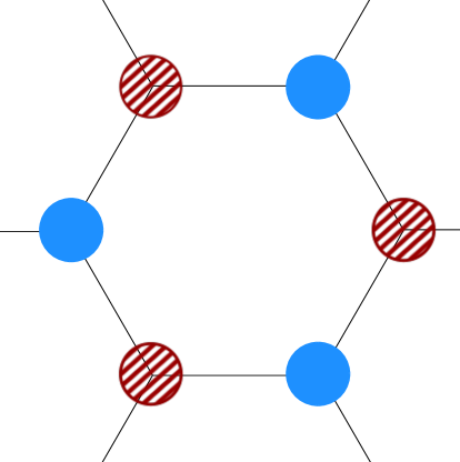
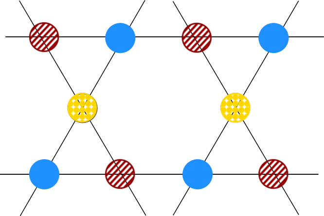
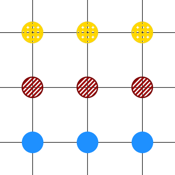
Figure 2: Sublattice orderings for several common lattices. The sublattices are distinguished by different colors (shadings). Left: Two sublattice ordering in a honeycomb lattice. The sublattices are stable with respect to all spatial symmetries. Middle: Three sublattice ordering on a kagome lattice. The sublattices are stable with respect to all spatial symmetries. Right: Three sublattice ordering on a square lattice. The sublattices are stable with respect to all translational symmetries, horizontal and vertical reflections, $180^{\circ}$ rotations but not with respect to $90^{\circ}$ rotations or diagonal reflections.

III.1 Sublattice coding on two sublattices

For demonstration purposes, we consider a simple translationally invariant spin-$1/2$ system on a six-site chain lattice with periodic boundary conditions. The lattice is divided into two sublattices as in Fig. 1. The even sites form the sublattice $A$ and the odd sites form the sublattice $B$. We enumerate the sites such that the sites $1$ to $3$ are in sublattice $A$ and the sites $4$ to $6$ are in sublattice $B$. We choose the integer representation of a state $\ket{\bm{\sigma}}$ such that the most significant bits are formed by the spins in sublattice $A$. The symmetry group we consider consists of the six translations on the chain

$$\mathcal{G}=\{\text{Id},T,T_{2},T_{3},T_{4},T_{5}\},$$ (8)

where $T_{n}$ denotes the translation by $n$ lattice sites. The splitting of the lattice into two sublattices is stable in the sense that every symmetry element $g\in\mathcal{G}$ either maps the $A$ sublattice to $A$ and the $B$ sublattice to $B$ or the $A$ sublattice to $B$ and the $B$ sublattice to $A$. We call this property sublattice stability. It is both a property of the partition of our lattice into sublattices and the symmetry group. Hence, the symmetry group is composed of two kinds of symmetries

$$\begin{split}\mathcal{G}_{A}&\equiv\{g\in\mathcal{G}\,;\quad g\text{ maps sublattice }A\text{ onto }A\},\\ \mathcal{G}_{B}&\equiv\{g\in\mathcal{G}\,;\quad g\text{ maps sublattice }B\text{ onto }A\}.\end{split}$$ (9)

We denote by $\ket{\bm{\sigma}}_{A}$ (resp. $\ket{\bm{\sigma}}_{B}$) the state restricted to sublattice $A$ (resp. $B$) and define the sublattice representatives,

$$\begin{split}\texttt{Rep}_{A}(\ket{\bm{\sigma}}_{A})&\equiv h_{A}\ket{\bm{\sigma}}_{A},\quad h_{A}=\operatornamewithlimits{argmin}_{g\in\mathcal{G}_{A}}\,\text{int}(g\ket{\bm{\sigma}}_{A}),\\ \texttt{Rep}_{B}(\ket{\bm{\sigma}}_{B})&\equiv h_{B}\ket{\bm{\sigma}}_{B},\quad h_{B}=\operatornamewithlimits{argmin}_{g\in\mathcal{G}_{B}}\,\text{int}(g\ket{\bm{\sigma}}_{B}),\end{split}$$ (10)

and the representative symmetries,

$$\begin{split}\texttt{Sym}_{A}(\ket{\bm{\sigma}}_{A})&\equiv\{g\in\mathcal{G}_{A}\,;\quad{g}\ket{\bm{\sigma}}_{A}=\texttt{Rep}_{A}(\ket{\bm{\sigma}}_{A})\},\\ \texttt{Sym}_{B}(\ket{\bm{\sigma}}_{B})&\equiv\{g\in\mathcal{G}_{B}\,;\quad{g}\ket{\bm{\sigma}}_{B}=\texttt{Rep}_{B}(\ket{\bm{\sigma}}_{B})\}.\end{split}$$ (11)

Let again $\ket{\tilde{\bm{\sigma}}}=g_{\bm{\sigma}}\ket{\bm{\sigma}}$, where $\ket{\tilde{\bm{\sigma}}}$ is the representative of $\ket{\bm{\sigma}}$. The minimizing symmetry $g_{\bm{\sigma}}$ can only be an element of $\texttt{Sym}_{A}(\ket{\bm{\sigma}}_{A})$ if $\texttt{Rep}_{A}(\ket{\bm{\sigma}}_{A})\leq\texttt{Rep}_{B}(\ket{\bm{\sigma}}_{B})$, or vice versa. Put differently,

$$\texttt{Rep}_{B}(\ket{\bm{\sigma}}_{B})<\texttt{Rep}_{A}(\ket{\bm{\sigma}}_{A})\quad\Rightarrow\quad g_{\bm{\sigma}}\notin\texttt{Sym}_{A}(\ket{\bm{\sigma}}_{A}).$$ (12)

Otherwise, any symmetry element in $\texttt{Rep}_{B}(\ket{\bm{\sigma}}_{B})$ would yield a smaller integer value than $g_{\bm{\sigma}}$. This is the core idea behind the sublattice coding technique. We store $\texttt{Rep}_{A,B}(\ket{\bm{\sigma}}_{A,B})$ for every substate $\ket{\bm{\sigma}}_{A,B}$ in a lookup table together with $\texttt{Sym}_{A,B}(\ket{\bm{\sigma}}_{A,B})$. In a first step, we determine the sublattice representative with smallest most significant bits. Then we apply the representative symmetries to $\ket{\bm{\sigma}}$ in order to determine the true representative $\ket{\tilde{\bm{\sigma}}}$. The number of representative symmetries $|\texttt{Sym}_{A,B}(\ket{\bm{\sigma}}_{A,B})|$ is typically much smaller than the total number of symmetries $|\mathcal{G}|$. The following example illustrates the idea and shows how to compute the representative given the information about sublattice representatives and representative symmetries.

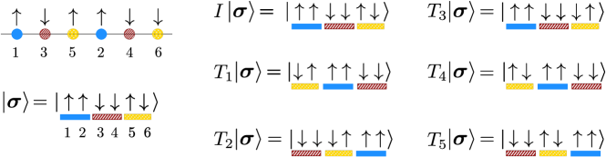
Figure 3: Three sublattice coding of the spin state $\ket{\bm{\sigma}}$ on a six-site chain lattice and action of translation symmetries. The sites are enumerated such that site $1$ and $2$ are on sublattice $A$ (blue, solid), $3$,$4$ on $B$ (red, dashed) and $5$,$6$ on $C$ (yellow, dotted). The representative state with this enumeration of sites is given by $\ket{\tilde{\bm{\sigma}}}=T_{2}\ket{\bm{\sigma}}=\ket{\downarrow\downarrow\downarrow\uparrow\uparrow\uparrow}$

Example

We consider the state $\ket{\bm{\sigma}}=\ket{\uparrow\uparrow\downarrow\downarrow\uparrow\downarrow}$ on a six-site chain lattice as in Fig. 1. Notice that the sites are not enumerated from left to right but such that sites $1$ to $3$ belong to the sublattice $A$ and sites $4$ to $6$ belong to sublattice $B$. The states restricted on the sublattices are $\ket{\bm{\sigma}}_{A}=\ket{\uparrow\uparrow\downarrow}$ and $\ket{\bm{\sigma}}_{B}=\ket{\downarrow\uparrow\downarrow}$. The action of the sublattice symmetries

$$\begin{split}\mathcal{G}_{A}&\equiv\{\text{Id},T_{2},T_{4}\},\\ \mathcal{G}_{B}&\equiv\{T_{1},T_{3},T_{5}\},\\ \end{split}$$ (13)

on $\ket{\bm{\sigma}}$ is shown in Fig. 1. From this, we compute the sublattice representatives as in Eq. 10,

$$\begin{split}\texttt{Rep}_{A}(\ket{\bm{\sigma}}_{A})&=\ket{\downarrow\uparrow\uparrow},\\ \texttt{Rep}_{B}(\ket{\bm{\sigma}}_{B})&=\ket{\downarrow\downarrow\uparrow},\end{split}$$ (14)

whose integer values are given by

$$\begin{split}\operatorname{int}(\texttt{Rep}_{A}(\ket{\bm{\sigma}}_{A}))&=(011)_{2}=3,\\ \operatorname{int}(\texttt{Rep}_{B}(\ket{\bm{\sigma}}_{B}))&=(001)_{2}=1.\end{split}$$ (15)

Since $\texttt{Rep}_{B}(\ket{\bm{\sigma}}_{B})<\texttt{Rep}_{A}(\ket{\bm{\sigma}}_{A})$ the symmetry $g_{\bm{\sigma}}$ yielding the total representative $\ket{\tilde{\bm{\sigma}}}$ must be contained in

$$\texttt{Sym}_{B}(\ket{\bm{\sigma}}_{B})=\{T_{1}\},$$ (16)

which in this case just contains a single element, namely $T_{1}$. Consequently, the representative $\ket{\tilde{\bm{\sigma}}}$ is given by

$$\ket{\tilde{\bm{\sigma}}}=T_{1}\ket{\bm{\sigma}}=\ket{\downarrow\downarrow\uparrow\uparrow\uparrow\downarrow}.$$ (17)

Lookup tables

If the quantities $\texttt{Rep}_{A,B}(\ket{\bm{\sigma}}_{A,B})$ and $\texttt{Sym}_{A,B}(\ket{\bm{\sigma}}_{A,B})$ are now stored in a lookup table, this computation can be done very efficiently. Notice that instead of having to store $2^{N}$ entries in the lookup table for the representative we only need four lookup tables of order $\mathcal{O}(2^{N/2})$, two for the quantities $\texttt{Rep}_{A}(\ket{\bm{\sigma}}_{A})$ and $\texttt{Rep}_{B}(\ket{\bm{\sigma}}_{B})$, and two for $\texttt{Sym}_{A}(\ket{\bm{\sigma}}_{A})$ and $\texttt{Sym}_{B}(\ket{\bm{\sigma}}_{B})$. On larger system sizes the difference between memory requirements of order $\mathcal{O}(2^{N})$ and $\mathcal{O}(2^{N/2})$ is substantial.

To further speed up computations we also create lookup tables to store the action of each symmetry $g\in\mathcal{G}$ on a substate $\ket{\bm{\sigma}}_{A}$,

$$\begin{split}\texttt{SymmetryAction}_{A}(g,\ket{\bm{\sigma}}_{A})&={g}\ket{\bm{\sigma}}_{A},\\ \texttt{SymmetryAction}_{B}(g,\ket{\bm{\sigma}}_{B})&={g}\ket{\bm{\sigma}}_{B}.\end{split}$$ (18)

With this information, we can efficiently apply symmetries to a given spin configuration by looking up the action of $g$ on the respective substate and combining the results. The memory requirement for these lookup tables is $\mathcal{O}(N_{\text{sym}}2^{N/2})$, where $N_{\text{sym}}=|\mathcal{G}|$. This can be reduced by generalizing the sublattice coding algorithm to multiple sublattices, as explained in the following section. In that case, $2N_{\text{sublat}}$ lookup tables of size $\mathcal{O}(2^{N/N_{\text{sublat}}})$ are required for storing the sublattice representatives $\texttt{Rep}_{X}(\ket{\bm{\sigma}}_{X})$ and representative symmetries $\texttt{Sym}_{X}(\ket{\bm{\sigma}}_{X})$, as defined in Eqs. 21 and 22, respectively. $N_{\text{sublat}}$ denotes the number of sublattices. For storing the action of each symmetry $\texttt{SymmetryAction}_{X}(g,\ket{\bm{\sigma}}_{X})$ as in Eq. 23 we further need $N_{\text{sublat}}$ lookup tables of size $\mathcal{O}(N_{\text{sym}}2^{N/N_{\text{sublat}}})$.

III.2 Generic sublattice coding algorithm

We start by discussing how we subdivide a lattice $\Lambda$ into $N_{\text{sublat}}$ sublattices. The basic requirement is that every symmetry group element either only operates within the sublattices or exchanges sublattices. We do not allow for symmetry elements that split up a sublattice onto different sublattices. Therefore we make the following definition:

Definition (Sublattice stability)

A decomposition,

$$\Lambda=\mathop{\vphantom{\bigcup}\mathchoice{\leavevmode\vtop{\halign{\hfil$\m@th\displaystyle#$\hfil\cr\bigcup\cr\cdot\crcr}}}{\leavevmode\vtop{\halign{\hfil$\m@th\textstyle#$\hfil\cr\bigcup\cr\cdot\crcr}}}{\leavevmode\vtop{\halign{\hfil$\m@th\scriptstyle#$\hfil\cr\bigcup\cr\cdot\crcr}}}{\leavevmode\vtop{\halign{\hfil$\m@th\scriptscriptstyle#$\hfil\cr\bigcup\cr\cdot\crcr}}}}\displaylimits\limits_{X=1}^{N_{\text{sublat}}}\Lambda_{X},$$ (19)

of a lattice $\Lambda$ with symmetry group $\mathcal{G}$ into $N_{\text{sublat}}$ disjoint sublattices $\Lambda_{X}$ is called sublattice stable if every $g\in\mathcal{G}$ maps each $\Lambda_{X}$ onto exactly one (possibly different) $\Lambda_{Y}$, i.e. for all $g\in\mathcal{G}$ and all $\Lambda_{X}$ there exists a $\Lambda_{Y}$ such that

$$g(\Lambda_{X})=\Lambda_{Y}.$$

The set $\Lambda_{X}$ is called the $X$-sublattice of $\Lambda$.

The notion of sublattice stability is illustrated in Fig. 2. The sublattices $\Lambda_{X}$ are drawn in different colors (shadings). A translation by one unit cell keeps the sublattices of the honeycomb lattice invariant whereas a $60^{\circ}$ rotation exchanges the sublattices. For the kagome lattice in Fig. 2 a $60^{\circ}$ rotation around a hexagon center for example cyclically permutes the three sublattices. One checks that for both the honeycomb and the kagome lattice in Fig. 2 all translational as well as all point group symmetries are sublattice stable, so different color (shading) sublattices are mapped onto each other. This is different for the square lattice in Fig. 2. Still here all translational symmetries just permute the sublattices, but a $90^{\circ}$ rotation splits up a sublattice into different sublattices. Nevertheless, a $180^{\circ}$ rotation keeps the sublattices stable, similarly a vertical or horizontal reflection. Therefore, only the reduced point group $\mathrm{D}2$ instead of the full $\mathrm{D}4$ point group for the square lattice fulfills the sublattice stability condition in this case. $\mathrm{D}2$ and $\mathrm{D}4$ denote the dihedral groups of order $4$ and $8$ with two- and four-fold rotations and reflections. Note, that for a square lattice a two or four sublattice decomposition for which the full $\mathrm{D}4$ point group is sublattice stable can be chosen instead. The choice of this particular sublattice decomposition just serves illustrational purposes.

From the definition of sublattice stability, it is clear that the total number of sites $N$ has to be divisible by the number of sublattices $N_{\text{sublat}}$. The numbering of the lattice sites is chosen such that the lattice sites from $(X-1)N/N_{\text{sublat}}+1$ to $XN/N_{\text{sublat}}$ belong to sublattice $X$. We choose the most significant bits in the integer representation to be the bits on sublattice $1$. Similar as in the previous section we define the following quantities

Definition

For every sublattice $\Lambda_{X}$ we define the following notions:

• sublattice symmetries:

  $$\mathcal{G}_{X}\equiv\{g\in\mathcal{G}\,|\,g\text{ maps sublattice }X\text{ onto sublattice }1\}.$$ (20)

• sublattice representative:

  $$\texttt{Rep}_{X}(\ket{\bm{\sigma}}_{X})\equiv h_{X}\ket{\bm{\sigma}}_{X},\quad h_{X}=\operatornamewithlimits{argmin}_{g\in\mathcal{G}_{X}}\,\text{int}(g\ket{\bm{\sigma}}_{X}),$$ (21)

  where $\ket{\bm{\sigma}}_{X}$ denotes the substate of $\ket{\bm{\sigma}}$ restricted on sublattice $\Lambda_{X}$.

• representative symmetries:

  $$\texttt{Sym}_{X}(\ket{\bm{\sigma}}_{X})\equiv\{g\in\mathcal{G}_{X}\,|\,{g}\ket{\bm{\sigma}}_{X}=\texttt{Rep}_{X}(\ket{\bm{\sigma}}_{X})\}.$$ (22)

• sublattice symmetry action:

  $$\texttt{SymmetryAction}_{X}(g,\ket{\bm{\sigma}}_{X})={g}\ket{\bm{\sigma}}_{X}.$$ (23)

The symmetries in $\mathcal{G}_{X}$ map the sublattice $X$ onto the most significant bits. Therefore, the symmetry that minimizes the integer value in the orbit must be contained in the representative symmetries of a minimal sublattice representative, i.e.

$$g_{\bm{\sigma}}=\operatornamewithlimits{argmin}\limits_{g\in\mathcal{G}}{g}\ket{\bm{\sigma}}\Rightarrow g_{\bm{\sigma}}\in\bigcup\limits_{\begin{subarray}{c}Y\text{, {Rep}}_{Y}(\ket{\bm{\sigma}}_{Y})\\ \text{minimal}\end{subarray}}{\texttt{Sym}}_{Y}(\ket{\bm{\sigma}}_{Y}).$$ (24)

To find the minimizing symmetry $g_{\bm{\sigma}}$, we only have to check the symmetries yielding the minimal sublattice representative. The quantities $\texttt{Rep}_{X}(\ket{\bm{\sigma}}_{X})$ and $\texttt{Sym}_{X}(\ket{\bm{\sigma}}_{X})$ are stored in lookup tables, whose size scales as $\mathcal{O}(2^{N/N_{\text{sublat}}})$. In order to quickly apply the symmetries, we can additionally store $\texttt{SymmetryAction}_{X}(g,\ket{\bm{\sigma}}_{X})$ in another lookup table. The memory cost of doing so scales as $\mathcal{O}(N_{\text{sym}}2^{N/N_{\text{sublat}}})$ and thus requires the most memory. The generic sublattice coding algorithm consists of two parts. The preparation of the lookup tables is shown as pseudocode in algorithm 1. The pseudocode of the actual algorithm for finding the representative using the lookup tables is shown in algorithm 2.

Algorithm 1 Preparation of lookup tables for sublattice coding algorithm

for each substate $\ket{\bm{\sigma}_{X}}$ :

     for each sublattice $X$ :

         compute $\texttt{Rep}_{X}(\ket{\bm{\sigma}}_{X})$ Eq. 21, store it

         compute $\texttt{Sym}_{X}(\ket{\bm{\sigma}}_{X})$ Eq. 22, store them

         for each symmetry $g\in\mathcal{G}$ :

              compute $\texttt{SymmetryAction}_{X}(g,\ket{\bm{\sigma}}_{X})$, store it               

Algorithm 2 Sublattice coding algorithm for finding the representative.

state $\ket{\bm{\sigma}}$

representative $\ket{\tilde{\bm{\sigma}}}$ and $g_{\bm{\sigma}}$

Determine $\texttt{MinRep}=\min\limits_{X}\left\{\texttt{Rep}_{X}(\ket{\bm{\sigma}}_{X})\right\}$

Set $\ket{\tilde{\bm{\sigma}}}=+\infty$

for each sublattice $Y$ with $\texttt{Rep}_{Y}(\ket{\bm{\sigma}}_{Y})=\texttt{MinRep}$ :

     for each symmetry $g\in\texttt{Sym}_{Y}(\ket{\bm{\sigma}}_{Y})$ :

         compute ${g}\ket{\bm{\sigma}}$ from $\texttt{SymmetryAction}_{X}(g,\ket{\bm{\sigma}}_{X})$

         if ${g}\ket{\bm{\sigma}}<\ket{\tilde{\bm{\sigma}}}$ :

              $\ket{\tilde{\bm{\sigma}}}\leftarrow{g}\ket{\bm{\sigma}}$

              $g_{\bm{\sigma}}\leftarrow{g}$               

return $\ket{\tilde{\bm{\sigma}}}$, $g_{\bm{\sigma}}$

Example

We consider the same state on a six-site chain lattice as in Fig. 1, but now using a three sublattice decomposition in Fig. 3. We call the blue (solid) sublattice the $A$ sublattice, the red (dashed) $B$ and the yellow (dotted) $C$. Notice, that due to different sublattice structure the labeling of the real space sites is different from the two sublattice case. In the three sublattice case, we are now given the state

$$\ket{\bm{\sigma}}=\ket{\uparrow\uparrow\downarrow\downarrow\uparrow\downarrow}.$$ (25)

Its substates are

$$\begin{split}\ket{\bm{\sigma}}_{A}=\ket{\uparrow\uparrow},\\ \ket{\bm{\sigma}}_{B}=\ket{\downarrow\downarrow},\\ \ket{\bm{\sigma}}_{C}=\ket{\uparrow\downarrow},\end{split}$$ (26)

with corresponding sublattice representatives

$$\begin{split}\texttt{Rep}_{A}(\ket{\bm{\sigma}}_{A})=\ket{\uparrow\uparrow},\\ \texttt{Rep}_{B}(\ket{\bm{\sigma}}_{B})=\ket{\downarrow\downarrow},\\ \texttt{Rep}_{C}(\ket{\bm{\sigma}}_{C})=\ket{\downarrow\uparrow},\end{split}$$ (27)

and representative symmetries

$$\begin{split}\texttt{Sym}_{A}(\ket{\bm{\sigma}}_{A})=\{I,T_{3}\},\\ \texttt{Sym}_{B}(\ket{\bm{\sigma}}_{B})=\{T_{2},T_{5}\},\\ \texttt{Sym}_{C}(\ket{\bm{\sigma}}_{C})=\{T_{1}\}.\end{split}$$ (28)

The minimal sublattice representative MinRep as in algorithm 2 is given by

$$\texttt{MinRep}=\texttt{Rep}_{B}(\ket{\bm{\sigma}}_{B})=\ket{\downarrow\downarrow}.$$ (29)

The minimizing symmetry must now be in $\texttt{Sym}_{B}(\ket{\bm{\sigma}}_{B})=\{T_{2},T_{5}\}$. We see that

$$T_{2}\ket{\bm{\sigma}}=\ket{\downarrow\downarrow\downarrow\uparrow\uparrow\uparrow}<T_{5}\ket{\bm{\sigma}}=\ket{\downarrow\downarrow\uparrow\downarrow\uparrow\uparrow}.$$ (30)

Therefore, the representative $\ket{\tilde{\bm{\sigma}}}$ is given by

$$\ket{\tilde{\bm{\sigma}}}=\ket{\downarrow\downarrow\downarrow\uparrow\uparrow\uparrow},$$ (31)

with the minimizing symmetry $g_{\bm{\sigma}}=T_{2}$. Notice, that this state differs from the one found in the two sublattice example since the labeling of the sites changes the integer representation of a state and thus the definition of the representative. Once a given labeling of sites is fixed the representative is of course unique.

IV Distributed and hybrid memory parallelization

For reaching larger system sizes in ED computations a proper balance between memory requirements and computational costs has to be found. There are two major approaches when applying the Lanczos algorithm. The Hamiltonian matrix can either be stored in memory in some sparse-matrix format or generated on-the-fly every time a matrix-vector multiplication is performed. Storing the matrix is usually faster, yet memory requirements are higher. This approach is for example pursued by the software package SPINPACK Schulenburg (2017). A matrix-free implementation of the Lanczos algorithm usually needs more computational time since the matrix generation, especially in a symmetrized basis can be expensive. Of course, the memory cost is drastically reduced since only a few vectors of the size of the Hilbert space have to be stored. It turns out that on current supercomputing infrastructures the main limitation in going to larger system sizes is indeed the memory requirements of the computation. It is thus often favorable to use a slower matrix-free implementation, as done by the software package ${\mathcal{H}}\Phi$ Kawamura et al. (2017), for example. Due to this reasons, we also choose the matrix-free approach.

The most computational time in the Lanczos algorithm is used in the matrix-vector multiplication. The remaining types of operations are scalar multiplications, dot products of Lanczos vectors or the diagonalization of the $T$-matrix which are usually of negligible computational cost. Today’s largest supercomputers are typically distributed memory machines, where every process only has direct access to a small part of the total memory. It is thus a nontrivial task to distribute data onto several processes and implement communication amongst them once remote memory has to be accessed. Also, when scaling the software to a larger amount of processes load balancing becomes important. The computational work should be evenly distributed amongst the individual processes in order to avoid waiting times in communication. In the following, we explain how we achieve this goal in our implementation using the Message Passing Protocol (MPI).

Matrix-vector multiplication

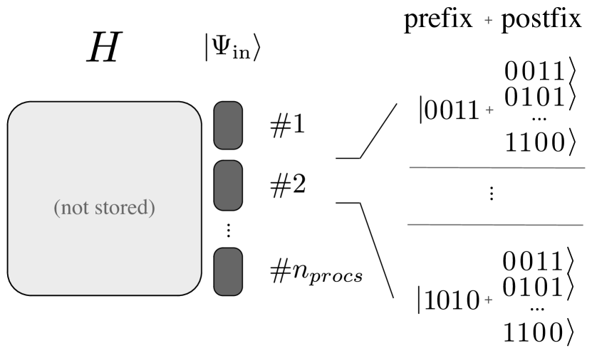
Figure 4: Storage layout of the distributed Hilbert space. The prefixes are randomly distributed amongst the MPI processes using a hash function. States with same prefixes are mapped to the same process. Within a process, the states are ordered lexicographically. The Hamiltonian matrix is not stored.

The Hamiltonian can be written a sum of non-branching terms,

$$H=\sum\limits_{k}H_{k}.$$ (32)

To perform the full matrix-vector multiplication we compute the matrix-vector multiplication for the non-branching terms $H_{k}$ and add up the results,

$$H\ket{\psi}=\sum\limits_{k}H_{k}\ket{\psi}.$$ (33)

We denote by

$$\{\ket{\bm{\sigma}_{i}}\},\quad i=1,\ldots,D\quad,$$ (34)

a (possibly symmetry-adapted) basis of the Hilbert space. A wave function $\ket{\psi}$ is represented on the computer by storing its coefficients $\braket{\bm{\sigma}_{i}}{\psi}$. Given an input vector,

$$\ket{\psi_{\text{in}}}=\sum\limits_{i=1}^{D}\braket{\bm{\sigma}_{i}}{\psi_{\text{in}}}\ket{\bm{\sigma}_{i}},$$ (35)

we want to compute the coefficients $\braket{\bm{\sigma}_{i}}{\psi_{\text{out}}}$ in

$$H_{k}\ket{\psi_{\text{in}}}=\ket{\psi_{\text{out}}}.$$ (36)

The resulting output vector $\ket{\psi_{\text{out}}}$ is given by

$$\begin{split}\ket{\psi_{\text{out}}}&=\sum\limits_{i=1}^{D}\braket{\bm{\sigma}_{i}}{\psi_{\text{out}}}\ket{\bm{\sigma}_{i}}=\sum\limits_{i=1}^{D}\braket{\bm{\sigma}_{i}}{H_{k}}{\psi_{\text{in}}}\ket{\bm{\sigma}_{i}}\\ &=\sum\limits_{i,j=1}^{D}c_{k}(\bm{\sigma}_{j})\braket{\bm{\sigma}_{j}}{\psi_{\text{in}}}\braket{\bm{\sigma}_{i}}{\bm{\sigma}_{j}^{\prime}}\ket{\bm{\sigma}_{i}},\end{split}$$ (37)

where $c_{k}(\bm{\sigma}_{j})$ and $\ket{\bm{\sigma}_{j}^{\prime}}$ are given by

$$H_{k}\ket{\bm{\sigma}_{j}}=c_{k}(\bm{\sigma}_{j})\ket{\bm{\sigma}_{j}^{\prime}}.$$ (38)

Notice, that in a symmetry-adapted basis, evaluating $c_{k}(\bm{\sigma}_{j})$ requires the evaluation of Eq. 6, where the sublattice coding technique can be applied. Clearly, we have

$$\braket{\bm{\sigma}_{i}}{\bm{\sigma}_{j}^{\prime}}=\begin{cases}1\text{ if }\ket{\bm{\sigma}_{i}}=\ket{\bm{\sigma}_{j}^{\prime}},\\ 0\text{ else.}\end{cases}$$ (39)

For parallelizing the multiplication Eq. 37, we distribute the coefficients in the basis $\{\ket{\bm{\sigma}_{i}}\}$ onto the different MPI processes. This means we have a mapping,

$$\texttt{proc}:\ket{\bm{\sigma}_{i}}\rightarrow\{1,\dots,n_{\text{procs}}\},$$ (40)

that assigns to every basis state of the Hilbert space its MPI process number. Here, $n_{\text{procs}}$ denotes the number of MPI processes. In general, $\ket{\bm{\sigma}_{j}}$ and $\ket{\bm{\sigma}_{j}^{\prime}}$ are not stored in the same process. Hence, the coefficient $c_{k}(\bm{\sigma}_{j})\braket{\bm{\sigma}_{j}}{\psi_{\text{in}}}$ has to be sent from the process no. $\texttt{proc}(\ket{\bm{\sigma}_{j}})$ to process no. $\texttt{proc}(\ket{\bm{\sigma}_{j}^{\prime}})$. This makes communication between the processes necessary. This communication is buffered in our implementation, i.e. for every basis state $\ket{\bm{\sigma}_{j}}$ we first store the target basis state $\ket{\bm{\sigma}_{j}^{\prime}}$ and the coefficient $c_{k}(\bm{\sigma}_{j})\braket{\bm{\sigma}_{j}}{\psi_{\text{in}}}$ locally. Once every local basis state has been evaluated, we perform the communication and exchange the information amongst all processes. This corresponds to an MPI_Alltoallv call in the MPI standard.

After this communication step, every process has to add the received coefficient to the locally stored coefficient $\braket{\bm{\sigma}_{j}^{\prime}}{\psi_{\text{out}}}$. For this, we have to search, where the now locally stored coefficient of the basis state $\ket{\bm{\sigma}_{j}^{\prime}}$ is located in memory. Typically, we keep a list of all locally stored basis states defining the position of the coefficients. This list is then searched for the entry $\ket{\bm{\sigma}_{j}^{\prime}}$, which can also be time-consuming and needs to be done efficiently. We are thus facing the following challenges when distributing the basis states of the Hilbert space amongst the MPI processes:

• Every process has to know which process any basis state $\ket{\bm{\sigma}_{i}}$ belongs to.

• The storage of the information about the distribution should be memory efficient.

• The distribution of basis states has to be fair, in the sense that every process has a comparable workload in every matrix-vector multiplication.

• The search for a basis state within a process should be done efficiently.

We now propose a method to address these issues in a satisfactory way.

Distribution of basis states

The central point of our parallelization strategy is the proper choice of the distribution function $\texttt{proc}(\bm{\sigma})$ for the basis states in Eq. 40. We split up every basis state into prefix and postfix sites,

$$\ket{\bm{\sigma}}=\ket{\underbrace{\sigma_{1}\cdots\sigma_{n_{\text{prefix}}}}_{\text{prefix sites}}\quad\underbrace{\sigma_{n_{\text{prefix}}+1}\cdots\sigma_{n_{\text{prefix}}+n_{\text{postfix}}}}_{\text{postfix sites}}},$$ (41)

where $n_{\text{prefix}}$ and $n_{\text{postfix}}$ denote the number of prefix and postfix sites. We decide that states with the same prefix are stored in the same MPI process. The prefixes are randomly distributed amongst all the processes. We do this by using a hash function that maps the prefix bits onto a random but deterministic MPI process. This hash function can be chosen such that every process has a comparable amount of states stored locally. Moreover, a random distribution of states reduces load balance problems significantly since the communication structure is randomized. This is in stark contrast to distributing the basis states in a linear fashion. Thereby, single processes can often have a multiple of the workload than other processes, thus causing idle time in other processes.

Algorithm 3 Preparation of the distributed and symmetrized Hilbert space

Perform the following steps on every process in parallel (no communication necessary)

myid denotes the number of the current MPI process

prepares data structures Basis, Limits on each process

for each prefix spin configuration $\ket{\bm{\sigma}_{\text{prefix}}}=\ket{\sigma_{1}\cdots\sigma_{n_{\text{prefix}}}}$ :

     if $\texttt{proc}(\ket{\bm{\sigma}_{\text{prefix}}})\neq$ myid :

         continue

     else:

         begin = length(Basis)

         for each spin configuration $\ket{\bm{\sigma}}$ with prefix $\ket{\bm{\sigma}_{\text{prefix}}}$ :

              compute representative $\ket{\tilde{\bm{\sigma}}}$ of $\ket{\bm{\sigma}}$

              if $\ket{\bm{\sigma}}=\ket{\tilde{\bm{\sigma}}}$ :

                  append $\ket{\bm{\sigma}}$ to Basis                        end = length(Basis)

         if end $\neq$ begin :

              insert ($\ket{\bm{\sigma}_{\text{prefix}}}$, begin, end) to Limits               

Algorithm 4 Parallel matrix-vector multiply for a non-branching term $H_{k}$

input wave function $\ket{\psi_{\text{in}}}$

matrix-vector product $\ket{\psi_{\text{out}}}=H_{k}\ket{\psi_{\text{in}}}$

$\rhd$ Preparation and sending step (communication may be buffered)

for each basis state $\ket{\bm{\sigma}_{j}}$ stored locally in Basis :

     $\cdot$ apply non-branching $H_{k}$ and use sublattice coding technique to compute $c_{k}(\bm{\sigma}_{j})$ and $\ket{\bm{\sigma}_{j}^{\prime}}$,

$$H_{k}\ket{\bm{\sigma}_{j}}=c_{k}(\bm{\sigma}_{j})\ket{\bm{\sigma}_{j}^{\prime}}.$$

     $\cdot$ compute $c=c_{k}(\bm{\sigma}_{j})\braket{\bm{\sigma}_{j}}{\psi_{\text{in}}}$

     $\cdot$ send the pair $(\ket{{\bm{\sigma}}_{j}^{\prime}},c)$ to process no. $\texttt{proc}(\ket{{\bm{\sigma}}_{j}^{\prime}})$

$\rhd$ Receiving and search step

for each pair $(\ket{{\bm{\sigma}}_{j}^{\prime}},c)$ received :

     $\cdot$ determine indices (begin, end) from $\texttt{Limits}(\ket{{\bm{\sigma}}_{j}^{\prime}})$

     $\cdot$ determine index $i$ of $\ket{\bm{\sigma}^{\prime}}$ by binary search in array Basis between (begin, end)

     $\cdot$ Set $\braket{\bm{\sigma}_{j}^{\prime}}{\psi_{\text{out}}}[i]\leftarrow c$

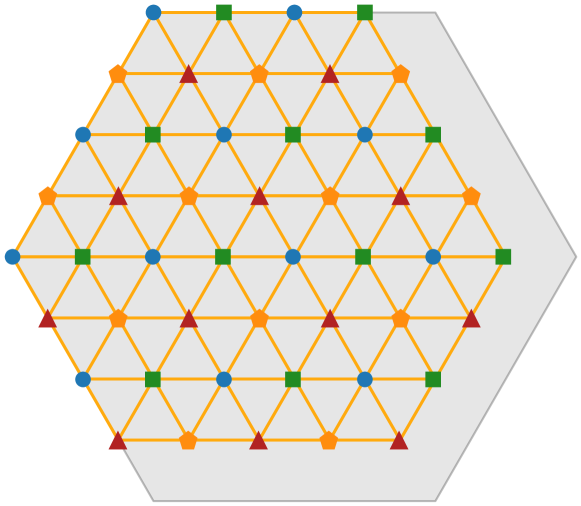
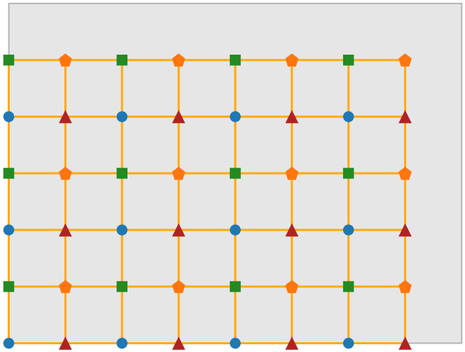
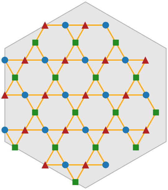
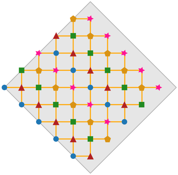
Figure 5: Geometries of Heisenberg spin-$1/2$ model benchmarks. Different colors (symbols) show the sublattice structure used for the sublattice coding technique. Grey background shows the Wigner-Seitz cell defining the periodicity of the lattice. Left: Triangular lattice, $48$ sites, four sublattice structure. Middle left: Square lattice, $48$ sites, four sublattice structure. Middle right: Kagome lattice, $48$ sites, three sublattice structure. Right: Square lattice, $50$ sites, five sublattice structure.

By choosing this kind of random distribution of basis states, we also don’t have to store any information about their distribution. This information is all encoded in the hash function. Nevertheless, we store the basis states belonging to a process locally in an array. Finding the index of a given basis state also requires some computational effort. Here, we use the separation between prefix and postfix sites. We store the basis states in an ordered way. This way, states belonging to the same prefix are aligned in memory as shown in Fig. 4. We can store the index of the first and the last states that belong to a given prefix. To find the index of a given state we can now lookup the first and last index of the prefix of this state and perform a binary search for the state between these two indices. This reduces the length of the array we have to perform the binary search on and, hence, reduces the computational effort in finding the index. For implementing this procedure we need two data structures locally stored on each process.

1. An array $\texttt{Basis}(i)$ storing all the basis states,

   $$\texttt{Basis}(i)=\ket{\bm{\sigma}_{i}},\quad i=1,\ldots,D.$$ (42)

2. An associative array $\texttt{Limits}(\ket{\bm{\sigma}_{\text{prefix}}})$ storing the map

   $$\texttt{Limits}(\ket{\bm{\sigma}_{\text{prefix}}})=\left[\texttt{begin}(\ket{\bm{\sigma}_{\text{prefix}}}),\texttt{end}(\ket{\bm{\sigma}_{\text{prefix}}})\right]$$ (43)

   where $\texttt{begin}(\ket{\bm{\sigma}_{\text{prefix}}})$ denotes the index of the first state with prefix $\ket{\bm{\sigma}_{\text{prefix}}}$ and $\texttt{end}(\ket{\bm{\sigma}_{\text{prefix}}})$ denotes the index of the last state with this prefix in the array $\texttt{Basis}(i)$, $\ket{\bm{\sigma}_{\text{prefix}}}=\ket{\sigma_{1}\cdots\sigma_{n_{\text{prefix}}}}$.

In algorithm 3 we summarize how to prepare these data structures. The parallel matrix-vector multiplication in pseudocode is shown in algorithm 4. When working in the symmetry-adapted basis, the lookup tables of the sublattice coding method need to be accessible to every MPI process. One way to achieve this is of course, that every process generates its own lookup tables. However, in present-day supercomputers, several processes will be assigned to the same physical machine sharing the same physical memory. To save memory, the lookup tables are stored only once on a computing node. Its processes can then access the lookup tables via shared memory access. In our code, we use POSIX shared memory functions pos (2017) to implement this hybrid parallelization.

V Benchmarks

In order to assess the power of the methods proposed in the previous sections, we performed test runs to compute ground state energies. We considered the Heisenberg antiferromagnetic spin-$1/2$ nearest neighbor model,

$$H=J\sum\limits_{\langle i,j\rangle}\bm{S}_{i}\cdot\bm{S}_{j},\quad J=1,$$ (44)

on four different lattice geometries: square ($48$ sites), triangular ($48$ sites), kagome ($48$ sites) and square ($50$ sites). Fig. 5 shows the simulation clusters and the sublattice structure we used. The benchmarks were performed on three different supercomputers. The Vienna Scientific Cluster VSC3 is built up from over 2020 nodes with two Intel Xeon E5-2650v2, 2.6 GHz, 8 core processors, the supercomputer Hydra at the Max Planck Supercomputing & Data Facility in Garching with over 3500 nodes with 20 core Intel Ivy Bridge 2.8 GHz processors and the System B Sekirei at the Institute for Solid State Physics of the University of Tokyo with over 1584 nodes with two Intel Xeon E5-2680v3 12 core 2.5GHz processors. Both the Hydra and Sekirei use InfiniBand FDR interconnect, whereas the VSC3 uses Intel TrueScale Infiniband for network communication.

The benchmarks are summarized in table 1. We make use of all translational, certain point group symmetries and spin-flip symmetry. We show the memory occupied by a single lookup table for the symmetries. Since we use a single buffered and blocking all-to-all communication in the implementation it is straightforward to measure the percentage of time spent for MPI communication by taking the time before the communication call and afterward. In order to validate the results of our computation, we compared the results of the unfrustrated square case to Quantum Monte Carlo computations of the ground state energy. We used a continuous time world-line Monte Carlo Code Todo and Kato (2001) with $10^{5}$ thermalization and $10^{6}$ measurements at temperature $T=0.01$. The computed energies per site are $E/N=-0.676013\pm 2\cdot 10^{-5}$ for the $48$ site square cluster and $E/N=-0.67512\pm 2\cdot 10^{-5}$ for the $50$ site cluster. The actual values computed with ED are within the error bars. The ground state energy of the kagome Heisenberg antiferromagnet on $48$ sites has been previously computed Läuchli et al. (2016) with a specialized code and agrees with our results. We see that the amount of time spent for communication is different for the three supercomputers. On Sekirei, a parallel efficiency of $61\%$ on 3456 cores has been achieved.

Results for running the same problem on various numbers of processors are shown in Fig. 6. We chose two different problems for two sets of number of cores, the Heisenberg antiferromagnet with additional next-nearest neighbour and third nearest neighbour interactions on a $40$ site square lattice and the Heisenberg antiferromagnet on a $48$ site triangular lattice. We observe almost ideal scaling behaviour up to $4096$ MPI processes. Hence, the parallelization strategy described above successfully solves load balancing problems in the MPI communication. This benchmark has been performed on the Curie supercomputer at GENCI-TGCC-CEA, France.

Geometry	Triangular 48	Square 48	Kagome 48	Square 50
computer	Sekirei	VSC3	Hydra	Sekirei
point group	D6	D2	D6	D2
No. of symmetries	1152	384	384	400
dimension	$2.8\cdot 10^{10}$	$8.3\cdot 10^{10}$	$8.4\cdot 10^{10}$	$3.2\cdot 10^{11}$
No. of cores	3456	8192	10240	3456
total memory	2.5 TB	n.A.	n.A.	15.5 TB
memory lookup	151 MB	50 MB	604 MB	17 MB
Time / MVM	399 s	1241 s	258 s	3304 s
% comm. time	39%	77%	48%	39%
g.s. sector	$\Gamma$.A1.even	$\Gamma$.A1.even	$\Gamma$.A1.even	M.A1.odd
g.s. energy	-26.8129452715	-32.4473598728	-21.0577870635	-33.7551019315

Table 1: Benchmark results for various problems on three different supercomputer systems described in the main text. The employed symmetries include translational, point group and spinflip symmetry. We show the total memory used by all MPI processes and the memory used by the lookup tables for the sublattice coding technique. We also show the amount of time spent for communication. For labeling the ground state representations $\Gamma$ denotes the $(0,0)$ and $M$ the $(\pi,\pi)$ point in the Brillouin zone. A1 denotes the trivial point group representation and even/odd denotes the spinflip symmetry representation.

Figure 6: Scaling behaviour of the parallelization. The time for one matrix-vector multiplication in seconds is compared for the total number of processes. Both axes are scaled logarithmically. The matrix is the Hamiltonian of the Heisenberg spin $1/2$ antiferromagnet on a $40$ site cluster with additional next-nearest neighbour and third-nearest neighbour interactions for the benchmark on $16$, $64$, $128$ and $256$ cores. For $1024$, $2048$ and $4096$ cores the matrix is the Hamiltonian of the Heisenberg spin $1/2$ antiferromagnet on a $48$ site triangular cluster. The Hamiltonian is considered in its ground state sector. We observe almost ideal scaling behaviour up to $4096$ processors.

VI Discussion

The sublattice coding technique presented in section II allows for fast and memory-efficient evaluation of the matrix elements in a symmetry-adapted basis Eq. 6. Still, the construction of the sublattices imposes restrictions on the geometry of the simulation cluster. A sublattice construction with $N_{\text{sublat}}$ sublattices at least requires the number of sites to be divisible by $N_{\text{sublat}}$. The sublattice coding technique yields no advantages for lattice samples that have a prime number of sites. For lattices with several basis sites per unit cell a natural sublattice decomposition exists. The sublattices are given by the lattices defined by the corresponding basis sites. This is the case for the honeycomb and kagome lattice, where a natural two (resp. three) sublattice decomposition exists, cf. Fig. 2.

The sublattice decomposition for a given lattice is not unique. This can be seen in the case of the $50$ site square lattice, whose five sublattice decomposition is shown in Fig. 5. As a bipartite square lattice, it also allows for a two-sublattice decomposition. Three- and four-sublattice decompositions exist for other square lattice clusters as well (see e.g. Fig. 5). Hence, for a given simulation cluster there may exist more than one sublattice decomposition. Most of the high symmetry square and triangular lattice samples possess at least one sublattice decomposition in two or more sublattices. Still, a given sublattice decomposition may restrict the symmetry group if certain symmetry elements split up sublattices. This is, for example, the case for the $50$ site square lattice in Fig. 5. While the cluster itself has a full four-fold rotational and reflectional symmetry, the $90^{\circ}$ rotation is not sublattice stable. Therefore, only the $180^{\circ}$ rotation and reflection symmetry has been used as point group symmteries in the computation.

Increasing the number of sublattices decreases the memory required for storing the lookup tables. The computational effort for computing the representative as in algorithm 2 increases linearly in the number of sublattices. Also, smaller sublattices yield more potential representative symmetries Eq. 22 that have to be applied to the spin configuration. In principle, there is no restriction on the number of sublattices and the proper choice depends on the geometry of the simulation cluster, the available memory, and the desired speed. Fewer sublattices allow algorithm 2 to evaluate matrix elements faster.

The method of distributing the basis states of the Hilbert space is independent of the sublattice coding algorithm. Hence, this kind of parallelization can also be applied to problems without symmetries, like disordered systems. All information about the distribution of basis states is encoded by the hash function, that can be of rather simple type to achieve a balanced distribution.

One main motivation for performing large-scale ED computations is reaching system sizes for which high symmetry clusters are available. The possibility to simulate $48$ spin-$1/2$ particles gives access to the interesting triangular and kagome lattices shown in Fig. 5. These samples both have full sixfold rotational and reflectional symmetry. In reciprocal space, these clusters both accommodate the $K$ point and even the $M$ point for the triangular case. This feature is important to distinguish different phases with different ordering vectors. For the square lattice case, an interesting $52$ site cluster with four-fold rotational symmetry exists featuring the $(\pi,\pi)$ and $(\pi,0)$ point in reciprocal space. A study of the Heisenberg model with next-nearest neighbor interactions on this cluster can, therefore, yield valuable insights into nature of the intermediate phase, whose nature is not fully understood as of today. The methods proposed in this manuscript allow for these calculations on large present-day supercomputers, since the Hilbert space dimension of this problem is roughly four times larger than the investigated $50$ site case and a four sublattice decomposition is available.

Apart from spin systems, the sublattice coding algorithm also applies to fermionic systems, when the Hamiltonian is expressed in the occupation number basis. The occupation numbers of the orbitals on the respective sublattices define the sublattice configurations. In addition to computing a representative and representative symmetry, a Fermi sign has to be computed to evaluate matrix elements, which can be done efficiently.

VII Conclusion

We proposed the generic sublattice coding algorithm for making efficient use of discrete symmetries in large-scale ED computations. The method can be used flexibly on most lattice geometries and only requires a reasonable amount of memory for storing the lookup tables. The parallelization strategy for distributed memory architectures we discussed includes a random distribution of the Hilbert space amongst the parallel processes. Lookup tables of the sublattice coding technique are stored only once per node and are accessed via shared memory. Using these techniques, we showed that computations of spin-$1/2$ models of up to 50 spins have now become feasible.

References

- Gan and Harrison (2005) Z. Gan and R. J. Harrison, in Supercomputing, 2005. Proceedings of the ACM/IEEE SC 2005 Conference (2005) pp. 22–22.
- Sternberg et al. (2008) P. Sternberg, E. G. Ng, C. Yang, P. Maris, J. P. Vary, M. Sosonkina, and H. V. Le, in Proceedings of the 2008 ACM/IEEE Conference on Supercomputing, SC ’08 (IEEE Press, Piscataway, NJ, USA, 2008) pp. 15:1–15:12.
- Vary et al. (2009) J. P. Vary, P. Maris, E. Ng, C. Yang, and M. Sosonkina, Journal of Physics: Conference Series 180, 012083 (2009).
- Maris et al. (2010) P. Maris, M. Sosonkina, J. P. Vary, E. Ng, and C. Yang, Procedia Computer Science 1, 97 (2010), iCCS 2010.
- Rychkov and Vitale (2015) S. Rychkov and L. G. Vitale, Phys. Rev. D 91, 085011 (2015).
- Oitmaa and Betts (1978) J. Oitmaa and D. D. Betts, Can. J. Phys. 56, 897 (1978).
- Wietek and Läuchli (2017) A. Wietek and A. M. Läuchli, 95 (2017), 10.1103/PhysRevB.95.035141, arXiv:1604.07829 [cond-mat.str-el] .
- Wietek et al. (2015) A. Wietek, A. Sterdyniak, and A. M. Läuchli, 92 (2015), 10.1103/PhysRevB.92.125122, arXiv:1503.03389 [cond-mat.str-el] .
- Dagotto and Moreo (1989) E. Dagotto and A. Moreo, Phys. Rev. B 39, 4744 (1989).
- Leung and Elser (1993) P. W. Leung and V. Elser, Phys. Rev. B 47, 5459 (1993).
- Schulz, H.J. et al. (1996) Schulz, H.J. , Ziman, T.A.L. , and Poilblanc, D., J. Phys. (France) 6, 675 (1996).
- Richter and Schulenburg (2010) J. Richter and J. Schulenburg, Eur. Phys. J. B 73, 117 (2010).
- Läuchli et al. (2012) A. M. Läuchli, R. Johanni, and R. Moessner, “An exact diagonalization perspective on the kagome heisenberg antiferromagnet,” Talk, KITP Fragnets Program (2012).
- Läuchli et al. (2016) A. M. Läuchli, J. Sudan, and R. Moessner, arXiv E-prints , 1 (2016), arXiv:1611.06990 .
- Lin and Hirsch (1987) H. Q. Lin and J. E. Hirsch, Phys. Rev. B 35, 3359 (1987).
- Hasegawa and Poilblanc (1989) Y. Hasegawa and D. Poilblanc, Phys. Rev. B 40, 9035 (1989).
- Bonča et al. (1989) J. Bonča, P. Prelovšek, and I. Sega, Phys. Rev. B 39, 7074 (1989).
- Poilblanc (1995) D. Poilblanc, Phys. Rev. B 52, 9201 (1995).
- He et al. (1994) S. He, S. H. Simon, and B. I. Halperin, Phys. Rev. B 50, 1823 (1994).
- Morf et al. (2002) R. H. Morf, N. d’Ambrumenil, and S. Das Sarma, Phys. Rev. B 66, 075408 (2002).
- Neupert et al. (2011) T. Neupert, L. Santos, C. Chamon, and C. Mudry, Phys. Rev. Lett. 106, 236804 (2011).
- Läuchli et al. (2013) A. M. Läuchli, Z. Liu, E. J. Bergholtz, and R. Moessner, Phys. Rev. Lett. 111, 126802 (2013).
- Schuler et al. (2016) M. Schuler, S. Whitsitt, L.-P. Henry, S. Sachdev, and A. M. Läuchli, Phys. Rev. Lett. 117, 210401 (2016).
- Whitsitt et al. (2017) S. Whitsitt, M. Schuler, L.-P. Henry, A. M. Läuchli, and S. Sachdev, Phys. Rev. B 96, 035142 (2017).
- Lin (1990) H. Q. Lin, Phys. Rev. B 42, 6561 (1990).
- Weiße (2013) A. Weiße, Phys. Rev. E 87, 043305 (2013).
- Feynman (1982) R. P. Feynman, Int. J. Theor. Phys. 21, 467 (1982).
- Häffner et al. (2005) H. Häffner, W. Hänsel, C. F. Roos, J. Benhelm, D. Chek-al kar, M. Chwalla, T. Körber, U. D. Rapol, M. Riebe, P. O. Schmidt, C. Becher, O. Gühne, W. Dür, and R. Blatt, Nature 438, 643 EP (2005).
- Castelvecchi (2017) D. Castelvecchi, Nature 541, 9–10 (2017).
- Häner and Steiger (2017) T. Häner and D. S. Steiger, in Proceedings of the International Conference for High Performance Computing, Networking, Storage and Analysis, SC ’17 (ACM, New York, NY, USA, 2017) pp. 33:1–33:10.
- Pednault et al. (2017) E. Pednault, J. A. Gunnels, G. Nannicini, L. Horesh, T. Magerlein, E. Solomonik, and R. Wisnieff, ArXiv e-prints (2017), arXiv:1710.05867 [quant-ph] .
- Gheorghiu et al. (2017) A. Gheorghiu, T. Kapourniotis, and E. Kashefi, ArXiv e-prints (2017), arXiv:1709.06984 [quant-ph] .
- Lanczos (1950) C. Lanczos, J. Res. Natl. Bur. Stand. 45, 255 (1950).
- Landau (1988) E. L. L. Landau, L.D. Landau, E.M. Lifshitz, Lehrbuch der Theoretischen Physik, vol. III, Quantenmechanik, 8th edn (Akademie-Verlag, Berlin, 1988).
- Läuchli (2011) A. M. Läuchli, “Introduction to Frustrated Magnetism: Materials, Experiments, Theory,” (Springer, Berlin, Heidelberg, 2011) Chap. Numerical Simulations of Frustrated Systems, pp. 481–511.
- Schulenburg (2017) J. Schulenburg, “SPINPACK,” (2017).
- Kawamura et al. (2017) M. Kawamura, K. Yoshimi, T. Misawa, Y. Yamaji, S. Todo, and N. Kawashima, Comput. Phys. Commun. 217, 180 (2017).
- pos (2017) SHM_OVERVIEW(7) Linux Programmer’s Manual, 4th ed. (2017).
- Todo and Kato (2001) S. Todo and K. Kato, Phys. Rev. Lett. 87, 047203 (2001).