Quantum temporal steering in a dephasing channel with quantum criticality

Abstract

We investigate the quantum temporal steering (TS), i.e., a temporal analogue of Einstein-Podolsky-Rosen steering, in a dephasing channel which is modeled by a central spin half surrounded by a spin-1/2 XY chain where quantum phase transition happens. The TS parameter $S_{\text{TS}}$ and the TS weight $W_{\text{TS}}$ are employed to characterize the TS dynamics. We analytically obtain the dependence of $S_{\text{TS}}$ on the decoherence factor. The numerical results show an obvious suppression of $S_{\text{TS}}$ and $W_{\text{TS}}$ when the XY chain approaches to the critical point. In view of the significance of quantum channel, we develop a new concept, TS weight power, in order to quantify the capacity of the quantum channel in dominating TS behavior. This new quantity enables us to indicate the quantum criticality of the environment by the quantum correlation of TS in the coupled system.

I Introduction

Recently, the problems of quantum steering have attracted considerable interest theoretically and experimentally 1 ; 2 ; 5 ; 3 ; 4 ; 6 ; 7 ; 8 ; QYHe1 ; 9 ; 10 ; QYHe2 ; 11 ; 12 ; 14 ; 15 ; 16 ; 17 ; 18 ; 19 . In a bipartite system sharing entangled states, Einstein-Podolsky-Rosen (EPR) steering problems refer to the quantum nonlocal correlations which allows one of the subsystems to remotely prepare or steer the other one via local measurements. Apart from the fundamental significance of steering in quantum mechanics 1 ; 2 ; 5 ; 3 ; 4 ; 6 ; 7 ; 8 , there are lots of application motivations that EPR steering was thought to be the driving power of quantum cryptography and teleportation 9 ; 10 ; QYHe2 ; 11 . For example, steering allows quantum key distribution (QKD) if one party trusts his own devices but not that of the other party 11 . An obvious advantage of this steering-dominated scenario is easier to implement, when compared with the device-independent protocols 12 .

In order to detect steerability, several inequalities in terms of the sufficient conditions of steerability were employed 1 ; 2 ; 5 ; 3 , and such inequalities have been tested by several experiments 3 ; 4 ; 9 . Beyond inequalities, a range of possible measures were developed to quantify the amount of steering 14 , then the existence of steerability can be sufficiently and necessarily demonstrated. Very recently, a powerful measure named the steerable weight was proposed 15 ; 16 . In other respects, steerability was found to be equivalent to joint measurability 17 ; 18 . A close relationship between steerability and quantum-subchannel discrimination was discovered in 19 .

Instead of discussing spatially-separated systems, a novel and important direction is to consider the quantum steering in time, i.e., the so-called temporal steering (TS) 20 , which focuses on a single object at different times. In this frame, a system is sent to a distant receiver (say Bob) through a quantum channel, then a detector or manipulator (say Alice) can perform some operations including measurements on the system, before Bob receives the system and performs his measurement. The existence of nonzero TS indicates that the temporal correlations, accounting for how strong Alice’s choice of measurements at an initial time, can influence the final state captured by Bob. This kind of correlation can be detected by the TS inequality 20 ; 20-1 ; 20-2 , which also becomes a very useful tool in verifying the suitability of a quantum channel for a certain QKD process. Compared to the spatial steering inequalities, TS inequality presents a superior applicability that the entanglement-based scenarios are no longer necessary, and one can directly carry out the BB84 protocol and other related protocols.

In order to quantify TS, a concept of TS weight was introduced in the literature 21 , where the authors found that TS characterized by the weight can be used to define a sufficient and practical measure of strong non-Markovianity. Therefore, it also implies the evident dependence of TS dynamics on the properties of quantum channels. Another temporal steering quantify called temporal steering robustness was introduced in by Ku et al. Ku16 , where TS was used for testing magnetoreception. The TS problems were also studied experimentally in a phenomenologically designed channel 22 and in a proposed channel based on the spin-boson interaction without rotating-wave rotating approximations Xiong17 . In other aspects, TS was found intrinsically associated with realism and joint measurability 23 ; 24 . The hierarchy among the temporal inseparability, temporal steering, and macrorealism was found Ku17 . Moreover, there is a recent work which studies the spatial-temporal steering Chen17 ; Costa17 and applied for testing quantum correlations in quantum networks including biological nano-structures.

In this paper, we intensively investigate the influence of the quantum channel on the TS behavior. This is a particular problem in TS other than EPR steering, because the formation of the quantum correlation between the system’s initial and final state lies on the quantum-channel. Therefore, TS is sensitive to the characteristic of the channel, then an interesting question arises: How does the TS behave in a special environment where quantum phase transition (QPT) happens?

It is known that QPT takes place at zero temperature, at which the thermal fluctuations vanish. Therefore, quantum fluctuation plays the major role in QPT. At the critical point, a qualitative change occurs in the ground state and long-range correlation also develops. Actually, if QPTs appear in the surrounding, the coherence properties of the center system indeed suffer significance changes, e.g., it enhances the decoherence of the system quan ; Zhang ; XSMa ; BShao ; Yuan , accelerates the disentanglement Zhe07 and also helps to induce quantum correlations X.X.Yi ; QAi . Motivated by these, we will take into account the influence of the quantum criticality on the dynamics of quantum TS.

II Two-dimensional dephasing channel

Let us start from a general dephasing model. For a two-dimensional system, the two basis vectors $\left|1\right\rangle$ and $\left|0\right\rangle$ are chosen as the eigenstates of the Pauli operator $\sigma_{z}$ obeying $\sigma_{z}\left|1\right\rangle=\left|1\right\rangle$ and $\sigma_{z}\left|0\right\rangle=-\left|0\right\rangle$. The interaction Hamiltonian reads

$$H=\left|1\right\rangle\left\langle 1\right|\otimes H_{+}+\left|0\right\rangle\left\langle 0\right|\otimes H_{-},$$ (1)

where $H_{\pm}$ denotes the resulting Hamiltonian corresponding to the eigenvalues of the qubit system. Thus the time evolution operator becomes

$$U(t)=\left|1\right\rangle\left\langle 1\right|\otimes U_{+}(t)+\left|0\right\rangle\left\langle 0\right|\otimes U_{-}(t).$$ (2)

The initial state of the total system is assumed in a product form

$$\rho_{\text{tot}}(0)=\rho_{s}\left(0\right)\otimes\rho_{e}\left(0\right),$$ (3)

where the states $\rho_{s}$ and $\rho_{e}$ denote the system and environment state respectively. Under the time evolution defined in Eq. (2) we finally obtain the reduced density matrix of the system

$$\rho_{s}\left(t\right)=\left(\begin{array}[]{cc}\rho_{11}\left(0\right)&\rho_{12}\left(0\right)F_{t}^{\ast}\\ \rho_{21}\left(0\right)F_{t}&1-\rho_{11}\left(0\right)\end{array}\right),$$ (4)

where $\rho_{ij}\left(0\right)$ ($i,j=1,2$) denote the elements of the initial state of the system. The decoherence factor, defined by $F\left(t\right)=$Tr$\left[\rho_{e}\left(0\right)U_{+}^{\dagger}(t)U_{-}(t)\right]$, plays a key role in the dynamic process.

III System-bath Hamiltonian with quantum criticality

A spin-1/2 XY spin chain displays the surrounding system where rich QPTs happen, and the Hamiltonian reads

$$H_{e}=-\sum_{l=-M}^{M}\left(\frac{1+\gamma}{2}\sigma_{l}^{x}\sigma_{l+1}^{x}+\frac{1-\gamma}{2}\sigma_{l}^{y}\sigma_{l+1}^{y}+{\lambda}\sigma_{l}^{z}\right),$$ (5)

where ${\lambda}$ characterizes the strength of the transverse field, and $\gamma$ is the dimensionless anisotropy parameter. $\sigma_{l}^{\alpha}\left(\alpha=x,y,z\right)$ are the Pauli operators defined on the $l$-th site, and the total number of spins in the chain is $L=2M+1$. The periodic boundary condition $\sigma_{L+1}=\sigma_{1}$ is assumed here and we henceforth set $\hbar=1$.

This XY model becomes the transverse Ising chain for $\gamma=1$. The critical point is at $\left|\lambda_{c}\right|=1$. Before that, when $\left|\lambda\right|\ll 1$, there are doubly degenerate ground states with all spins pointing either up or down along the $x$ (or $y$) axis. Whereas, for large cases of $\left|\lambda\right|\gg 1$, the spins of ground state are polarized up along $z$ direction. Therefore, at the critical point $\left|\lambda_{c}\right|=1$, there is a fundamental change of the ground state. When the parameter $\gamma=0$, it is the XX model. There is a criticality region along the line between $\lambda=-1$ and $\lambda=1$.

If one characterizes the critical features in terms of a critical exponent $\nu$ defined by the correlation length $\delta=\left|\lambda-\lambda_{c}\right|^{-\nu}$. For any values of $\gamma$, quantum criticality occurs at the critical field $\lambda_{c}=1$. For the interval $0<\gamma\leq 1$ the model belongs to the Ising universality class corresponding to the critical exponent $\nu=1$, while for $\gamma=0$ the model belongs to the XX universality class with $\nu=1/2$ S.Sachdev .

Fortunately, this XY model can be calculated exactly. By combining Jordan-Wigner transformation via $\prod\nolimits_{k<l}\sigma_{k}^{z}\sigma_{l}^{+}=c_{l}$ and Fourier transformation via $d_{k}=\frac{1}{\sqrt{N}}\sum_{l=-M}^{M}e^{-i\frac{2\pi lk}{N}}c_{l}$ to the momentum space S.Sachdev , the Hamiltonian can be written in a diagonal form as YDWang ; Zhe07

$$H_{e}=\sum_{k>0}\left(\Omega_{k}e^{i\frac{\theta_{k}}{2}\tilde{\sigma}_{kx}}\sigma_{kz}e^{-i\frac{\theta_{k}}{2}\tilde{\sigma}_{kx}}\right)+({\lambda-1)}\tilde{\sigma}_{0z},$$ (6)

where we have used the following pseudospin operators $\tilde{\sigma}_{k\alpha}\left(\alpha=x,y,z\right)$ Anderson

$$\tilde{\sigma}_{kx} = d_{k}^{\dagger}d_{-k}^{\dagger}+d_{-k}d_{k},\left(k=1,2,...M\right)\$$

$$\tilde{\sigma}_{ky} = -id_{k}^{\dagger}d_{-k}^{\dagger}+id_{-k}d_{k},$$

$$\tilde{\sigma}_{kz} = d_{k}^{\dagger}d_{k}+d_{-k}^{\dagger}d_{-k}-1,$$

$$\tilde{\sigma}_{0z} = 2d_{0}^{\dagger}d_{0}-1,$$ (7)

and $d_{k}^{\dagger},d_{k}\{k=0,1,2,...\}$ denote the fermionic creation and annihilation operators in the momentum space, respectively. Here,

$$\Omega_{k} = -2\sqrt{[{\lambda}-\cos(2\pi k/L)]^{2}+\gamma^{2}\sin^{2}(2\pi k/L)},$$

$$\theta_{k} = \arcsin\left[\frac{2\gamma\sin\left(2\pi k/L\right)}{\Omega_{k}}\right].$$ (8)

When an auxiliary qubit system is transversely coupled to the chain through the interaction Hamiltonian described by

$$H_{I}={g\sigma}_{z}\sum_{l=-M}^{M}\sigma_{l}^{z},$$ (9)

where operator ${\sigma}_{z}$ displays the center qubit system, and $g$ denotes the coupling strength. Then the total Hamiltonian becomes $H=H_{e}+H_{I}$, where we safely ignore the free Hamiltonian of the auxiliary particle. The $H=\left|1\right\rangle\left\langle 1\right|\otimes H_{+}+\left|0\right\rangle\left\langle 0\right|\otimes H_{-}$ in Eq. (1) can be constructed, where $H_{\pm}$ can be obtained by replacing ${\lambda}$ with ${\lambda}_{\pm}={\lambda\pm g}$ in Eq. (6) and (8).

The evolution is described as:

$$U_{\pm}(t)=e^{i(1-{\lambda}_{\pm}{)}\tilde{\sigma}_{0z}t}\prod_{k>0}e^{i\frac{\theta_{k\pm}}{2}\tilde{\sigma}_{kx}}e^{-it\Omega_{k\pm}\tilde{\sigma}_{kz}}e^{-i\frac{\theta_{k\pm}}{2}\tilde{\sigma}_{kx}},$$ (10)

where the parameters $\Omega_{k,\pm}$ and $\theta_{k,\pm}$ can be obtained by replacing ${\lambda}$ with ${\lambda}_{\pm}={\lambda\pm g}$ in Eq. (8). When we focus on the dynamics of the center system by doing partial trace over the bath space, the decoherence factor $F_{t}$ ( $F^{*}_{t}$) appears at the non-diagonal element of the reduced density matrix of the system with the definition $F_{t}=\text{Tr}[\rho_{e}U^{\dagger}_{-}U_{+}]$, which characterizes the dynamics of the quantum coherence. If we assume that the initial state of the environment is the ground state of the XY spin chain

$$|\psi\rangle_{e}=|1\rangle_{k=0}\otimes_{k>0}e^{i\frac{\theta_{k}}{2}\sigma_{kx}}|1\rangle_{k}|1\rangle_{-k},$$ (11)

where it should be noted that the first term $|1\rangle_{k=0}$ is for the case $\lambda<1,$ while $\lambda\geq 1$, it should be $|0\rangle_{k=0}$. Subsequently we obtain the decoherence factor

$$F_{t} = e^{-2itg}\prod_{k>0}\{\cos\left(\Omega_{k,-}t\right)\cos\left(\Omega_{k,+}t\right)$$ (12)

$$+\sin\left(\Omega_{k,-}t\right)\sin\left(\Omega_{k,+}t\right)\cos\left(\theta_{k,+}-\theta_{k,-}\right)$$

$$+i\cos\left(\Omega_{k,-}t\right)\sin\left(\Omega_{k,+}t\right)\cos\theta_{k,+}$$

$$-i\sin\left(\Omega_{k,-}t\right)\cos\left(\Omega_{k,+}t\right)\cos\theta_{k,-}\},$$

By introducing a cutoff number $K_{c}$ at the thermodynamic limit $L\rightarrow\infty$ and the critical limit $\lambda\rightarrow 1$, the norm of the factor approximately decays with time as quan (see details in the methods):

$$\left|F\right|_{K_{c}}\approx e^{-R_{c}t^{2}},$$ (13)

with $R_{c}=16E\left(K_{c}\right)\gamma^{2}g^{2}\left(1-\lambda\right)^{-2}$ and $E(K_{c})=2\pi^{2}K_{c}(K_{c}+1)(2K_{c}+1)/(6L^{2})$. Even at some cases that the factor $E\left(K_{c}\right)\gamma^{2}g^{2}\rightarrow 0$, the decay of the $\left|F\left(t\right)\right|$ is still possible due to the vanishing denominator $\left(1-\lambda\right)^{2}$ near the critical point $\lambda_{c}=1$. This heuristic analysis approximately predicts a monotonic decoherence process near the critical point $\lambda_{c}=1$ for any values of $\gamma$, while, beyond the critical region, different dynamics will be found.

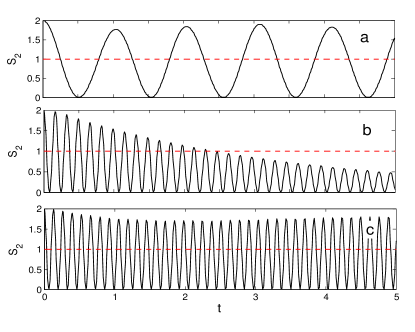
Figure 1: (Color online) Bidirectional-measurement TS parameter versus time $t$ for different parameters $\lambda=0.2,~{}1$ and $1.2$ presented in subfigures (a), (b) and (c), respectively. The parameter $\gamma=1$, the size of the surrounding spin chain is $L=1501$ and the system-bath coupling is $g=0.01$. The horizontal red dashed line denotes the steering limit. All the parameters are dimensionless throughout this paper. The time $t$ was rescaled dimensionless according to the coupling constants in all the following figures.

IV TS inequality and TS parameter

Let us briefly introduce a useful tool to detect steerability, i.e., the TS parameter $S_{N}$ which is derived from a temporal analogue of the steering inequality 20 ; 20-1 ,

$$S_{N}\equiv\sum\limits_{i=1}^{N}E\left(\left\langle B_{i,t_{B}}\right\rangle_{A_{i,t_{A}}}^{2}\right)\leq 1,$$ (14)

where $N$ ($=2$, $3$) is the number of mutually-unbiased measurements that Bob implements on his qubit and $A_{i,t_{A}}$ ($B_{i,t_{B}}$) stands for the $i_{\text{th}}$ observable measured by Alice (Bob) at $t_{A}$ ($t_{B}$). The violation of the above inequality indicates the existence of steerability, otherwise, it is not sure. In the definition of steering parameter $S_{N}$,

$$E\left(\left\langle B_{i,t_{B}}\right\rangle_{A_{i,t_{A}}}^{2}\right)\equiv\sum\limits_{a=\pm 1}P\left(A_{i,t_{A}}=a\right)\left\langle B_{i,t_{B}}\right\rangle_{A_{i,t_{A}}=a}^{2},$$ (15)

with $P\left(A_{i,t_{A}}=a\right)$ is the probability of the Alice’s measurement to receive the result of $a=+1$ or $-1$, and the Bob’s expectation value conditioned on Alice’s result defined as

$$\left\langle B_{i,t_{B}}\right\rangle_{A_{i,t_{A}}=a}\equiv\sum\limits_{b=\pm 1}bP\left(B_{i,t_{B}}=b|A_{i,t_{A}}=a\right),$$ (16)

where $P\left(B_{i,t_{B}}=b|A_{i,t_{A}}=a\right)$ denotes the condition probability of Bob’s measurement to get outcome $b$ (at time $t_{B}$) on the evolved state starting from the collapsed version as Alice’s measurement to get $a$ (at time $t_{A}$).

Let us take $N=2$ for example, Alice actually has a freedom to choose her measurement. Namely, the observables $A_{1,2}$($B_{1,2}$) can be any two of the Pauli operators $\sigma_{x,y,z}$, more generally, can be the operators consisting of the Pauli operators with arbitrary coefficients, as long as the direction of $A_{1}$($B_{1}$) is perpendicular to $A_{2}$($B_{2}$). Obviously one can expect that different measurements of Alice will produce different steerability, and which will be shown in the following sections. When associating TS with the error rate of a channel in BB84 protocol, the steering inequality bound and the BB84 threshold are found to be equivalent 20 . Namely, when $S_{2}$ [in Eq. (14) for $N=2$] becomes larger than $1$, both of the steerability and security of the channel will be verified. For a unitary evolution, there will always be $S_{2}>1$ in the whole duration, whereas, the quantum decoherence will significantly shorten the security time intervals 20 .

TS parameter in a two-dimensional dephasing channel. Now let us calculate the TS parameter based on an arbitrary choice of measurement pairs. By using two kinds of rotation: $U_{x,\theta}\equiv e^{i\frac{\theta}{2}\sigma_{x}}$, and $U_{y,\phi}\equiv e^{i\frac{\phi}{2}\sigma_{y}}$, the measurement bases can be described as $\left|\psi_{1}^{(+)}\right\rangle=U_{y,\phi}U_{x,\theta}\left|1\right\rangle$, $\left|\psi_{1}^{(-)}\right\rangle=U_{y,\phi}U_{x,\theta+\pi}\left|1\right\rangle$, $\left|\psi_{2}^{(+)}\right\rangle=U_{y,\phi}U_{x,\theta+\pi/2}\left|1\right\rangle$, and $\left|\psi_{2}^{(-)}\right\rangle=U_{y,\phi}U_{x,\theta+3\pi/2}\left|1\right\rangle$. Note that $\left|\psi_{1}^{(\pm)}\right\rangle$ are the eigenstates of the observable of $A_{1}$ and $\left|\psi_{2}^{(\pm)}\right\rangle$ are responsible for $A_{2}$. If we add a rotation around $\hat{z}$ axis to $\left|\psi_{2}^{(+)}\right\rangle$, it will turn to other directions on the plane perpendicular to $A_{1}$. Whereas, all the rotation around $\hat{z}$ direction causes no change to the TS parameter. By varying $\theta$ and $\phi$, one can reach the eigenstates corresponding to an arbitrary observable pair $\{A_{1},A_{2}\}$. When choosing the initial state of the system as a maximally mixed state, i.e., $\rho_{s}\left(0\right)=\mathbb{I}/2$, we obtain a general form of the TS parameter that

$$S_{2}=E_{1}+E_{2},$$ (17)

with the quantity:

$$E_{1} = P_{1}^{(+)}\left\{\text{Tr}\left[\left|\psi_{1}^{(+)}\right\rangle\left\langle\psi_{1}^{(+)}\right|\rho_{1t}^{(+)}\right]-\text{Tr}\left[\left|\psi_{1}^{(-)}\right\rangle\left\langle\psi_{1}^{(-)}\right|\rho_{1t}^{(+)}\right]\right\}^{2}$$

$$+P_{1}^{(-)}\left\{\text{Tr}\left[\left|\psi_{1}^{(+)}\right\rangle\left\langle\psi_{1}^{(+)}\right|\rho_{1t}^{(-)}\right]-\text{Tr}\left[\left|\psi_{1}^{(-)}\right\rangle\left\langle\psi_{1}^{(-)}\right|\rho_{1t}^{(-)}\right]\right\}^{2},$$

where $P_{1}^{(\pm)}=$Tr$\left[\left|\psi_{1}^{(\pm)}\right\rangle\left\langle\psi_{1}^{(\pm)}\right|\rho_{s}\left(0\right)\right]$ denotes the probability of Alice’s measurement on the initial state of the system and $\rho_{1t}^{(\pm)}$ displays the evolved state from $\left|\psi_{1}^{(\pm)}\right\rangle\left\langle\psi_{1}^{(\pm)}\right|$ under the quantum channel, consequently, we have

$$E_{1}=\left[\cos^{2}\theta\cos^{2}\phi\left(1-\text{Re}F_{t}\right)+\text{Re}F_{t}\right]^{2},$$ (19)

with $F_{t}$ corresponding to the decoherence factor causing by the dephasing channel in Eq. (4). Similarly, over the state $\left|\psi_{2}^{(\pm)}\right\rangle$, one can obtain

$$E_{2}=\left[\sin^{2}\theta\cos^{2}\phi\left(1-\text{Re}F_{t}\right)+\text{Re}F_{t}\right]^{2}.$$ (20)

We shall emphasize that the above expressions generally demonstrate the dependence of the TS parameter $S_{2}$ on the decoherence factor in a dephasing channel. Different values of $\theta$ and $\phi$ reflect the contribution of different measurement choices on $S_{2}$. Obviously, $S_{2}$ can reach its maximal value when $\theta$ and $\phi$ are set to satisfy $\sin 2\theta=0$ and $\sin\phi=0$, namely, $A_{1}=\sigma_{z}$ and $A_{2}=\sigma_{y}$ (or $\sigma_{x}$), and thus

$$S_{2,\max}=1+\text{Re}^{2}F_{t}.$$ (21)

We can also consider the case of three measurements operated by Alice, then another observable $A_{3}$ is introduced, whose direction is perpendicular to both $A_{1}$ and $A_{2}$ and the corresponding eigenstates can be described as $\left|\psi_{3}^{(\pm)}\right\rangle=U_{y,\phi}\left|1\right\rangle$. Then we have the third quantity

$$E_{3}=\left(\cos^{2}\phi\text{Re}F_{t}+\sin^{2}\phi\right)^{2},$$ (22)

and thus the TS parameter becomes

$$S_{3}=E_{1}+E_{2}+E_{3},$$ (23)

For the case of $A_{1}=\sigma_{z}$, $A_{2}=\sigma_{y}$, and $A_{3}=\sigma_{x}$, we have the maximum

$$S_{3,\max}=1+2\text{Re}^{2}F_{t}.$$ (24)

Obviously, the maximal values of $S_{2,\max}$ and $S_{3,\max}$ are not less than $1$ and their dynamics are absolutely dominated by the real part of the decoherence factor, i.e., Re$F_{t}$, which implies that before Re$F_{t}$ decays to zero, proper observable pair of Alice such as $\left\{\sigma_{z},\sigma_{x}\right\}$ (or $\left\{\sigma_{z},\sigma_{y}\right\}$) make sure the existence of the bidirectional-measurement TS. Furthermore, a choice of the measurements $\left\{\sigma_{z},\sigma_{x},\sigma_{y}\right\}$ guarantees the persistence of the tridirectional-measurement TS. However, after a sufficiently long-time decoherence process, $S_{2,\max}$ and $S_{3,\max}$ will tend to $1$, then the existence of TS becomes not sure.

In Fig. 1, we plot TS parameter $S_{2}$ vs evolution time with a duration $t_{b}=5$. The parameter $\gamma=1$. The coupling parameter is chosen as $g=0.01$ throughout the following numerical calculations. The measurement bases are chosen as $\left|+\right\rangle$ ($\left|-\right\rangle$) and $\left|R\right\rangle$ ($\left|L\right\rangle$) which are the eigenstates of $\sigma_{x}$ and $\sigma_{y}$. This choice of measurement bases leads to a non-maximal $S_{2}$ and it behaves as an oscillation with time. We investigate the cases of $\lambda=0.2$, $1$ and $1.2$ in subfigures (a), (b) and (c), respectively. When the environment undergoes the criticality at $\lambda=1$ [see subfigure (b)], the peak values of TS are obviously suppressed below the steering limit ($S_{N,\text{Lim}}=1$ denoted by red dashed lines) after a certain time. Whereas, beyond the critical region [see subfigures (a) and (c)], $S_{2}$ periodically crosses the steering limit and the peak values keep higher than $S_{N,\text{Lim}}=1$. The above comparison of the dynamical behavior of $S_{2}$ reveals the significant influence of the quantum criticality of the environment on the TS property of the coupled system.

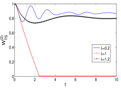
Figure 2: (Color online) Bidirectional-measurement TS weight versus time $t$ for different parameters $\lambda=0.2,~{}1$ and $1.2$. The parameter $\gamma=1$, the size of the surrounding spin chain is $L=1501$ and the system-bath coupling is $g=0.01$.

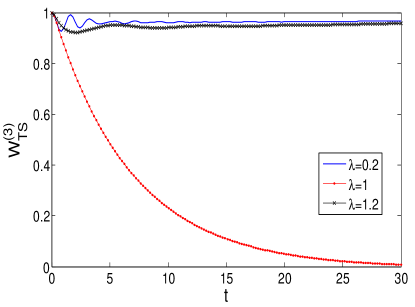
Figure 3: (Color online) Tridirectional-measurement TS weight versus time $t$ for different parameters $\lambda=0.2,~{}1$ and $1.2$. The parameter $\gamma=1$, the size of the surrounding spin chain is $L=1501$ and the system-bath coupling is $g=0.01$.

V TS weight and its power

TS weight. In order to precisely quantify the TS, a direct analogue of EPR steerable weight named TS weight is introduced via semidefinite programing as 21

$$W_{\text{TS}}^{(N)}\equiv 1-\max\text{ Tr}\sum\limits_{\lambda}^{m^{N}}\tilde{\sigma}_{\lambda},$$ (25)

subject to

$$\sigma_{a|A_{i}}-\sum\limits_{\lambda}D_{\lambda}\left(a|A_{i}\right)\tilde{\sigma}_{\lambda}\geq 0,\text{ \ }\forall a,A_{i},$$ (26)

and

$$\tilde{\sigma}_{\lambda}\geq 0,$$ (27)

where $\{\sigma_{a|A_{i}}\}$ stands for the assemblage received by Bob and whose origin is the resulting state after Alice’s measurements and a following evolution under a quantum channel. $N$ denotes the number of the observables measured by Alice and a $m$-dimensional operator $A_{i}$ ($i=1...N$) represents the $i_{\text{th}}$ observable chosen by Alice and $a$ is the measurement result. Then Bob only cares whether the assemblage he receives can be written in a hidden-state form 16 ; 21 , e.g., the second term in Eq. (26), where $\lambda$ indicates a local hidden variable, correspondingly, a set of semidefinite matrices $\tilde{\sigma}_{\lambda}$ act as the basis matrices, held by Bob, cooperating with the extremal deterministic single party conditional probability $D_{\lambda}\left(a|A_{i}\right)$. If there does not exists steerability between Alice’s and Bob’s system, at least one of the hidden-state form can be found to classically fabricate Alice’s measurement result. And thus $W_{\text{TS}}^{(N)}$ in Eq. (25) outputs a zero value. Otherwise, the steerability is sufficiently and necessarily verified.

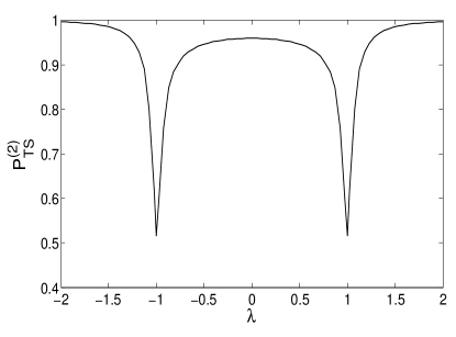
Figure 4: (Color online) Bidirectional-measurement TS weight power versus parameter $\lambda$ for $\gamma=1$. The evolution duration is bounded by $t_{b}=10$. The size of the surrounding spin chain is $L=1501$ and the system-bath coupling is $g=0.01$.

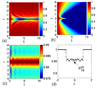
Figure 5: (Color online) Bidirectional-measurement TS weights versus both time $t$ and $\gamma$ are shown by the contours in subfigures (a), (b) and (c) corresponding to the cases $\lambda=0.2,~{}1$ and $1.2$, respectively. The size of the surrounding spin chain is $L=1501$ and the system-bath coupling is $g=0.01$. (d) presents the bidirectional-measurement TS weight power versus different $\lambda$ for the case of $\gamma=0.002$ (close to zero).

We numerically study a bidirectional-measurement TS weight $W_{\text{TS}}^{(2)}$ versus time $t$ for different field strengths of $\lambda=0.2$, $1$, and $1.2$ and show the results in Fig. 2. Our results clearly show that the quantum criticality in the environment seriously destroys the TS. When the parameter $\lambda$ is adjusted to the critical point $\lambda_{c}=1$, the TS weight $W_{\text{TS}}^{(2)}$ decays rapidly and displays a “sudden death”. This numerical result agrees well with the heuristic analysis of the decoherence factor in Eq. (13). Other cases beyond the critical region, such as $\lambda=0.2$ and $1.2$, $W_{\text{TS}}^{(2)}$ oscillates slightly around a high value about $0.9$ and $0.8$, respectively. Recalling the results in Fig. 1, after the time about $t>2.4$, the parameter $S_{2}$ becomes lower than $1$, however, it does not make sure whether there exists TS or not. Fortunately, the precise quantity $W_{\text{TS}}^{(2)}$ verifies the vanishment of TS.

In order to show the influence of different choices of measurement on the TS, in Fig. 3, we consider the tridirectional-measurement-induced TS characterized by $W_{\text{TS}}^{(3)}$. Differently, the quantum criticality suppresses $W_{\text{TS}}^{(3)}$ to zero asymptotically unlike the “sudden death” of $W_{\text{TS}}^{(2)}$ (in Fig. 2). Moreover, the decay rate is much more slowly than that of $W_{\text{TS}}^{(2)}$ (in Fig. 2). For the cases of $\lambda=0.2$ and $1.2$, the average values of $W_{\text{TS}}^{(3)}$ are obviously higher than these of $W_{\text{TS}}^{(2)}$ (in Fig. 2). Doing more measurements is generally helpful to capture more information of the target state, and thus it is expected to be beneficial for quantum steering. In the reference 16 , the authors numerically show the fact that increasing measurement direction numbers will increase quantum steering weight. Therefore, when the quantum decoherence is considered, the steering proposal with more measurement directions will be more robust to decoherence. Consequently, our results show that the steerability with two-directional measurements vanishes after a certain time (red line in Fig. 2). However, in the case of three-directional measurements, the steerability will keep non-zero values for quite a long time (red line in Fig. 3). We note that the sudden vanishing phenomena were found in several kinds of nonclassical effects Bartkowiak ; Miranowicz ; LiuYX ; WangXG ; Lambert ; MaJ .

On the other hand, from the analytical result of the decoherence factor in Eq. (12) and the approximate result in Eq. (13), one can find that only near the critical point, there is a monotonic decay of the quantum coherence. Other than that, the quantum coherence dynamics behaves like periodic function of time, which can be understood as the information periodically flow back to the system from the bath. Because of the close relationship between quantum coherence and steerability, the dramatic decoherence at the critical point leads to much lower steerability (red lines in Fig. 2 and Fig. 3) than those cases beyond the critical region (blue and black lines in Fig. 2 and Fig. 3).

TS weight power. In order to highlight the power of a quantum channel in influencing TS, we introduce a concept of TS weight power $P_{\text{TSW}}^{(N)}$ as

$$P_{\text{TSW}}^{(N)}\equiv\underset{\{A_{i}\}}{\max}\frac{1}{T_{b}}\int_{0}^{T_{b}}W_{\text{TS}}^{(N)}(t)\text{d}t,$$ (28)

where the maximalization is obtained over all the possible observables $A_{i}$ in an assemblage consists of $N$-directional measurements, then a time average is performed over an evolution duration $T_{b}$. In the definition of $P_{\text{TSW}}^{(N)}$, the influences of Alice’s choice of measurements and the temporal evolution on the steerability are technically covered, therefore, the role of the quantum channel becomes prominent.

In Fig. 4, we plot $P_{\text{TSW}}^{(2)}$ vs the coupling strength parameter $\lambda$ for the case of $\gamma=1$. By randomly choosing a sufficient number of observables along two directions, we numerically complete the maximization process in the definition of Eq. (28). From the results, the two minimum points precisely indicate the critical points of the environment.

When we take into account another values of $\gamma$, in Fig. 5, we plot $W_{\text{TS}}^{(2)}$ versus parameter $\gamma$ and time $t$ in subfigures (a), (b) and (c) corresponding to $\lambda=0.2$, $1$ and $1.2$, respectively. From the contour maps, one can clearly see the critical region drawn by $\gamma\rightarrow 0$. For a small parameter such as $\lambda=0.2$, the sudden death of TS appears only near the critical region $\gamma=0$. While, for the case $\lambda=1$ (a critical value), the phenomenon of the sudden death of TS exists for all the range of $\gamma$ as long as the evolution is long enough. This is consistent with the fact that for any values of $\gamma$, QPTs can occur at the critical point of $\lambda_{c}=1$. However, larger strength such as $\lambda=1.2$ prohibits the sudden death of TS for any values of $\gamma$. Instead, $W_{\text{TS}}^{(2)}$ displays weak oscillations around the values close to $1$. In order to clearly show the critical region, we calculate the power $P_{\text{TSW}}^{(2)}$ versus different $\lambda$ in the case of $\gamma=0.002$ (close to zero). When the environment undergoes the quantum critical region bounded by $\left|\lambda\right|\leq 1$, $P_{\text{TSW}}^{(2)}$ enters a disorder region which sensitively indicates the critical region.

VI Conclusion

In this paper, we have investigated the TS of a qubit surrounded by a XY spin chain where rich QPTs take place. The system-bath interaction has been assumed in a dephasing form, and the decoherence factor was obtained analytically. Based on this dephasing channel, we have given the analytical expression of the TS parameter which is directly dependent on the decoherence factor. Numerical results showed that at the critical point $\lambda=1$, the values of the TS parameter was obviously suppressed below the steering limit after a certain time. The disappearance of TS was confirmed when we took into account the TS weight. The sudden death of TS was found when the environment underwent its QPT. Finally, we have developed a new concept named TS weight power to quantify the capacity of the channel in influencing TS. With its help, the criticality of the environment can be clearly indicated. All of our analytical and numerical results reflect the significant influence of the quantum criticality on the TS dynamics. From another perspective, our results also reveal that the TS in such an auxiliary qubit can play as an effective tool to detect the QPTs of the surroundings. It still remains future interests of investigation on other quantum correlation dynamics in a wide variety of quantum-crical environments.

Appendix: Heuristic analysis of the decoherence factor

We calculate the norm of the decoherence factor,

$$\left|F_{t}\right| = \prod_{k>0}\left|F_{t}^{k}\right|$$

$$= \prod_{k>0}\big{\{}1-\big{[}\cos\left(t\Omega_{k,-}\right)\sin\left(t\Omega_{k,+}\right)\sin\alpha_{k,+}$$

$$-\sin\left(t\Omega_{k,-}\right)\cos\left(t\Omega_{k,+}\right)\sin\alpha_{k,-}\big{]}^{2}$$

$$-\sin^{2}\left(t\Omega_{k,+}\right)\sin^{2}\left(t\Omega_{k,-}\right)\sin^{2}\left(\alpha_{k,+}-\alpha_{k,-}\right)\big{\}}^{\frac{1}{2}},$$

where the parameters $\Omega_{k,\pm}$ and $\alpha_{k,\pm}=\theta_{k}-\theta_{k,\pm}$ can be obtained from Eq. (8) by replacing $\lambda$ with ${\lambda}_{\pm}={\lambda\pm g}$. Obviously, the values of $\left|F_{t}^{k}\right|$ are less than unit. Therefore, in the large $L$ limit, $\left|F_{t}\right|$ is expected to decay to zero.

By similar analysis of Ref. quan ; Zhe07 , we introduce a cutoff number $K_{c}$ to provide a lower bound of the norm of the decoherence factor as

$$\left|F_{t}\right|_{K_{c}}=\prod_{k>0}^{K_{c}}\left|F_{t}^{k}\right|\geq\left|F_{t}\right|,$$ (30)

therefore, we have the logarithmic form

$$S\left(t\right)=\ln\left|F_{t}\right|_{K_{c}}\equiv-\sum_{k>0}^{K_{c}}\left|\ln F_{t}^{k}\right|.$$ (31)

Now let us consider some conditions that $k$ is small enough, $L$ is very large, and $\gamma$ is a finite number, then we could omit some small terms in higher orders. Thus we have the following approximations: $\Omega_{k,\pm}\approx-2\left|1-{\lambda}_{\pm}\right|$, and $\sin\alpha_{k,\pm}\approx\pm 2g\gamma\pi k/\left(L\left|1-\lambda\right|\left|1-{\lambda}_{+}\right|\right)$ consequently $\sin\left(\alpha_{k,+}-\alpha_{k,-}\right)\approx 4g\gamma\pi k/\left(L\left|\left(1-{\lambda}_{+}\right)\left(1-\lambda_{-}\right)\right|\right)$. Furthermore, the approximated value of $S\left(t\right)$ reads

$$S\left(t\right) \approx -E\left(K_{c}\right)\left(1-{\lambda}_{+}\right)^{-2}\left(1-{\lambda}_{-}\right)^{-2}\left|1-\lambda\right|^{-2}\gamma^{2}g^{2}$$

$$\times\big{\{}4\sin^{2}\left(2t\left|1-\lambda_{+}\right|\right)\sin^{2}\left(2t\left|1-\lambda_{-}\right|\right)\left|1-\lambda\right|^{2}$$

$$+[\cos\left(2t\left|1-\lambda_{-}\right|\right)\sin\left(2t\left|1-\lambda_{+}\right|\right)\left|1-\lambda_{-}\right|$$

$$+\sin\left(2t\left|1-\lambda_{-}\right|\right)\cos\left(2t\left|1-\lambda_{+}\right|\right)\left|1-\lambda_{+}\right|]^{2}\big{\}},$$

where $E\left(K_{c}\right)=2\pi^{2}K_{c}\left(K_{c}+1\right)\left(2K_{c}+1\right)/\left(6L^{2}\right).$ Now let us consider a short time and a weak enough coupling $g$, when $\lambda$ approaches to $\lambda_{c}=1,$ there will be $S_{c}\left(t\right)\approx-16E\left(K_{c}\right)\gamma^{2}g^{2}\left[4t^{4}+t^{2}\left(1-\lambda\right)^{-2}\right]$.

Note that when $L\rightarrow\infty$ in thermodynamic limit, the parameter$\ E\left(K_{c}\right)$ should tend to $0$. In this case, due to the contribution of $\left(1-\lambda\right)^{-2}$, the terms with $t^{2}$ survive. Thus, the norm of the factor approximately behaves as

$$\left|F_{t}\right|_{K_{c}}\approx e^{-R_{c}t^{2}},$$ (33)

with a decay rate $R_{c}=16E\left(K_{c}\right)\gamma^{2}g^{2}\left(1-\lambda\right)^{-2}.$ In some cases that the factor $E\left(K_{c}\right)\gamma^{2}g^{2}$ approaches to$\ 0$, the decay of the $\left|F\left(t\right)\right|$ is still possible when the parameter enter the critical region, i.e., $\lambda\rightarrow 1$ due to the denominator $\left(1-\lambda\right)^{2}$. However, beyond the critical region, the decay of the bound $\left|F_{t}\right|_{K_{c}}$ will not be sure. Instead, it perhaps behave as an oscillation with time due to the periodic functions such as the $\sin\left(2t\left|1-\lambda_{+}\right|\right)$ in Eq. (LABEL:S). The analysis above reveals the fact that the remarkable decay of $\left|F\left(t\right)\right|$ corresponds to the occurrence of quantum criticality at the critical point $\lambda_{c}=1$ for any values of $\gamma$.

VII Acknowledgments

Z.S. is supported by the National Natural Science Foundation of China under Grant No. 11375003 and 11775065, the Program for HNUEYT under Grant No. 2011-01-011, the Zhejiang Natural Science Foundation with Grant Nos. LZ13A040002 and LY17A050003, the Ministry of Science and Technology of China under Grant No. 2016YFA0301802, the funds for the Hangzhou-City Quantum Information and Quantum Optics Innovation Research Team. B.L. acknowledges the Thirteenth Five-year Planning Project of Jilin Provincial Education Department Foundation under Grant No.JJKH20170650KJ. Y.H. acknowledges support by the Natural Science Foundation of Zhejiang province of China NO. LQ16A040001 and NSFC through Grant No. 11605157.

References

- (1) H. M. Wiseman, S. J. Jones, and A. C. Doherty, Phys. Rev. Lett. 98, 140402 (2007).
- (2) S. J. Jones, H. M. Wiseman, and A. C. Doherty, Phys. Rev. A 76, 052116 (2007).
- (3) E. G. Cavalcanti, S. J. Jones, H. M. Wiseman, and M. D. Reid, Phys. Rev. A 80, 032112 (2009).
- (4) D. Smith, G. Gillett, M. de Almeida, C. Branciard, A. Fedrizzi, T. Weinhold, A. Lita, B. Calkins, T. Gerrits, H. Wiseman, S. W. Nam, and A. White, Nat. Commun. 3, 625 (2012).
- (5) V. Handchen, T. Eberle, S. Steinlechner, A. Samblowski, T. Eberle, Torsten. Franz, R. F. Werner, and R. Schnabel, Phys. Rev. Lett. 6, 596 (2012).
- (6) K. Sun, X. J. Ye, J. S. Xu, X. Y. Xu, J. S. Tang, Y. C. Wu, J. L. Chen, C. F. Li, and G. C. Guo, Phys. Rev. Lett. 116, 160404 (2016).
- (7) Z. Y. Ou, C. F. Pereira, H. J. Kimble, and K. C. Peng, Phys. Rev. Lett. 68, 3663 (1992).
- (8) J. Bowles, T. Vértesi, M. T. Quintino, and N. Brunner, Phys. Rev. Lett. 112, 200402 (2014).
- (9) Q. Y. He, Q. H. Gong, and M. D. Reid, Phys. Rev. Lett. 114, 060402 (2015).
- (10) D. J. Saunders, S. J. Jones, H. M. Wiseman, and G. J. Pryde, Nat. Phys. 6, 845-849 (2010).
- (11) S. P. Walborn, A. Salles, R. M. Gomes, F. Toscano, and P. H. Souto Ribeiro, Phys. Rev. Lett. 106, 130402 (2011).
- (12) Q. Y. He, L. Rosales-Zarate, G. Adesso, and M. D. Reid, Phys. Rev. Lett. 115, 180502 (2015).
- (13) C. Branciard, E. G. Cavalcanti, S. P. Walborn, V. Scarani, and H. M. Wiseman, Phys. Rev. A 85, 010301(R) (2012).
- (14) A. Acin, N. Brunner, N. Gisin, S. Massar, S. Pironio, and V. Scarani, Phys. Rev. Lett. 98, 230501 (2007).
- (15) I. Kogias, A. R. Lee, S. Ragy, and G. Adesso, Phys. Rev. Lett. 114, 060403 (2015).
- (16) M. F. Pusey, Phys. Rev. A 88, 032313 (2013).
- (17) P. Skrzypczyk, M. Navascués, and D. Cavalcanti, Phys. Rev. Lett. 112, 180404 (2014).
- (18) M. T. Quintino, T. Vértesi, and N. Brunner, Phys. Rev. Lett. 113, 160402 (2014).
- (19) R. Uola, T. Moroder, and O. Gühne, Phys. Rev. Lett. 113, 160403 (2014).
- (20) M. Piani, and J. Watrous, Phys. Rev. Lett. 114, 060404 (2015).
- (21) Y. N. Chen, C. M. Li, N. Lambert, S. L. Chen, Y. Ota, G. Y. Chen, and F. Nori, Phys. Rev. A 89, 032112 (2014).
- (22) C. Emary, N. Lambert, and F. Nori, Rep. Prog. Phys. 77, 016001 (2014).
- (23) K. Bartkiewicz, A. Černoch, K. Lemr, A. Miranowicz, and F. Nori, Phys. Rev. A 93, 062345 (2016).
- (24) S. L. Chen, et al., Phys. Rev. Lett. 116, 020503 (2016).
- (25) H. Y. Ku, S. L. Chen, H. B. Chen, N. Lambert, Y. N. Chen, and F. Nori, Phys. Rev. A 94, 062126 (2016).
- (26) K. Bartkiewicz, A. Černoch, K. Lemr, A. Miranowicz, and F. Nori, Sci. Rep. 6, 38076 (2016).
- (27) S. J. Xiong, Y. Zhang, Z. Sun, L. Yu, Q. Su, X. Q. Xu, J. S. Jin, Q. Xu, J. M. Liu, K. Chen, and C. P. Yang, Optica 4, 1065 (2017).
- (28) C. M. Li, Y. N. Chen, N. Lambert, C. Y. Chiu, and F. Nori, Phys. Rev. A 92, 062310 (2015).
- (29) H. S. Karthik, J. Prabhu Tej, A. R. Usha Devi, and A. K. Rajagopal, J. Opt. Soc. Am. B 32, A34 (2015).
- (30) H. Y. Ku, S. L. Chen, N. Lambert, Y. N. Chen, and F. Nori, arXiv :1710.11387.
- (31) S. L. Chen, N. Lambert, C. M. Li, G. Y. Chen, Y. N. Chen, A. Miranowicz, and F. Nori, Sci. Rep. 7, 3728 (2017).
- (32) E. Costa, M. Ringbauer, M. E. Goggin, A. G. White, and A. Fedrizzi, arXiv :1710.01776.
- (33) H. T. Quan, Z. Song, X. F. Liu, P. Zanardi, and C. P. Sun, Phys. Rev. Lett. 96, 140604 (2006).
- (34) J. F. Zhang, X. H. Peng, N. Rajendran, and D. Suter, Phys. Rev. Lett. 100, 100501 (2008).
- (35) X. S. Ma, A. M. Wang, and Y. Cao, Phys. Rev. B 76, 155327 (2007).
- (36) B. Q. Liu, B. Shao, and J. Zou, Phys. Rev. A 80, 062322 (2009).
- (37) Z. G. Yuan, P. Zhang, and S. S. Li, Phys. Rev. A 76, 042118 (2007).
- (38) Z. Sun, X. G. Wang, and C. P. Sun, Phys. Rev. A 75, 062312 (2007).
- (39) X. X. Yi, H. T. Cui, and L. C. Wang, Phys. Rev. A 74, 054102 (2006).
- (40) Q. Ai, T. Shi, G. L. Long, and C. P. Sun, Phys. Rev. A 78, 022327 (2008).
- (41) S. Sachdev, Quantum Phase Transition (Cambridge University Press, Cambridge, 1999).
- (42) Y. D. Wang, F. Xue, Z. Song, and C. P. Sun, Phys. Rev. B 76, 174519 (2007).
- (43) P. W. Anderson, Phys. Rev. 112, 1900 (1958).
- (44) M. Bartkowiak, A. Miranowicz, X. G. Wang, Y. X. Liu, W. Leoński, and F. Nori, Phys. Rev. A 83, 053814 (2011).
- (45) A. Miranowicz, M. Bartkowiak, X. G. Wang, Y. X. Liu, and F. Nori, Phys. Rev. A 82, 013824 (2010).
- (46) Y. X. Liu, A. Miranowicz, G. B. Gao, J. Bajer, C. P. Sun, and F. Nori, Phys. Rev. A 82, 032101 (2010).
- (47) X. G. Wang, A. Miranowicz, Y. X. Liu, C. P. Sun, and F. Nori, Phys. Rev. A 81, 022106 (2010).
- (48) N. Lambert, Y. N. Chen, R. Johansson, and F. Nori, Phys. Rev. B 80, 165308 (2009).
- (49) J. Ma, X. G. Wang, C. P. Sun, and F. Nori, Phys. Rep. 509, 89 (2011).