Probing the isotropy of cosmic acceleration using different supernova samples

Abstract

Recent studies indicated that an anisotropic cosmic expansion may exist. In this paper, we use three data sets of type Ia supernovae (SNe Ia) to probe the isotropy of cosmic acceleration. For the Union2.1 data set, the direction and magnitude of the dipole are $(l=309.3^{\circ}{}^{+15.5^{\circ}}_{-15.7^{\circ}},\ b=-8.9^{\circ}{}^{+11.2^{\circ}}_{-9.8^{\circ}})$, and $\ A=(1.46\pm 0.56)\times 10^{-3}$ from dipole fitting method. The hemisphere comparison results are $\delta=0.20,l=352^{\circ},b=-9^{\circ}$. For the Constitution data set, the results are $(l=67.0^{\circ}{}^{+66.5^{\circ}}_{-66.2^{\circ}},\ b=-0.6^{\circ}{}^{+25.2^{\circ}}_{-26.3^{\circ}})$, and $\ A=(4.4\pm 5.0)\times 10^{-4}$ for dipole fitting and $\delta=0.56,l=141^{\circ},b=-11^{\circ}$ for hemisphere comparison. For the JLA data set, no significant dipolar or quadrupolar deviation is found. We find previous works using ($l,b,A$) directly as fitting parameters may get improper results. We also explore the effects of anisotropic distributions of coordinates and redshifts on the results using Monte-Carlo simulations. We find that the anisotropic distribution of coordinates can cause dipole directions and make dipole magnitude larger. Anisotropic distribution of redshifts is found to have no significant effect on dipole fitting results.

1 Introduction

Type Ia supernovae (SNe Ia) are ideal standard candles Phillips1993 . In 1998, the accelerating expansion of the Universe was discovered using the luminosity-redshift relation of SNe Ia Riess1998 ; Perlmutter1999 . The cosmological principle assumes that the Universe is homogeneous and isotropic at large scales. Based on the cosmological principle and numerous observational facts, the standard $\Lambda$CDM model has been established. It can be used to explain various observations.

However, it is worthy to examine the validity of the standard $\Lambda$CDM model Kroupa2013 ; Kroupa2012 ; Perivolaropoulos2014 ; Koyama2015 and its assumptions, namely the cosmological principle. Deviation from cosmic isotropy with high statistical confidence level would lead to a major paradigm shift. At present, the standard cosmology confronts some challenges. Observations on the large-scale structure of the Universe, such as “great cold spot” on cosmic microwave background (CMB) sky map Vielva2004 , alignment of lower multipoles in CMB power spectrum DeOliveira-Costa2004 ; Tegmark2003 , alignment of polarization directions of quasars in large scale Hutsemekers2005 , handedness of spiral galaxies Longo2009 , and spatial variation of the fine structure constant King2012 ; Mariano2012 , show that the Universe may be anisotropic.

The isotropy of the cosmic acceleration has been widely tested using SNe Ia. Generally, there are two different ways to study the possible anisotropy from SNe Ia. The first one is directly fitting the data to a specific anisotropic model (AM) Campanelli2011 ; Li2013 ; Wang2018 . Many anisotropic cosmological models have been proposed to match the observations, including the Bianchi I type cosmological model Campanelli2011 ; Aluri2013 and the Rinders-Finsler cosmological model Chang2014 . The extended topological quintessence model with a spherical inhomogeneous distribution for dark energy density is also proposed Mariano2012 .

An alternative method is directly analysing the SNe Ia data in a model-independent way Antoniou2010 ; Cai2012 ; Cai2013 ; Mariano2012 ; Zhao2013 ; Yang2013 ; Wang2014 ; Javanmardi2015 ; BeltranJimenez2015 ; Lin2016 ; Chang2018 ; Deng2018a ; Deng2018b ; Sun2018 , which does not depend on the specific cosmological model. The hemisphere comparison (HC) method and dipole fitting (DF) method are usually used in literature. The hemisphere comparison method divides samples into two hemispheres perpendicular to a polar axis, then fits cosmological parameters using samples in each hemisphere independently and compares their differences. The dipole fitting (DF) method assumes a dipolar deviation on redshift-distance modulus relation, then derives the dipole’s direction and magnitude using statistic approaches. Meanwhile, low-redshift SNe Ia are used to estimate the direction and amplitude of the local bulk flow Bonvin2006 ; Schwarz2007 ; Gordon2008 ; Colin2011 ; Turnbull2012 ; Kalus2013 ; Appleby2014 ; Huterer2015 . So far, no study has been able to rule out the isotropy at more than 3$\sigma$. The gravitational wave as standard siren has also been proposed to probe cosmic anisotropy Cai2018 .

The directions and magnitudes of anisotropy from previous works are shown in Table 1. It’s obvious that different results are derived from different authors. In this paper, we compare the DF fitting results of different SNe Ia samples and try to find the reason for the differences. This paper is organized as follows. In Section 2, SNe Ia data sets and DF method are introduced. The fitting results are shown in section 3.1. We discuss the possible reasons for the differences in Section 4. Finally, we summarize in Section 5.

2 Data and Methods

2.1 data sets

Large-scale systematic sky surveys on SNe Ia have been performed in the past decades. These surveys, which cover a wide range of redshifts from $z<0.1$ to $z\sim 1$, include Supernovae Legacy Survey (Astier2006, ; Sullivan2011, , SNLS), Sloan Supernova Survey Holtzman2008 , the Pan-STARRS survey Rest2013 ; Scolnic2013 ; Tonry2012 , Harvard-Smithsonian Center for Astrophysics survey (Hicken2009, , CfA), the Carnegie Supernova Project (Stritzinger2011, ; Folatelli2009, ; Contreras2009, , CSP), the Lick Observatory Supernova Search (Ganeshalingam2013, , LOSS), the Nearby Supernova Factory(Aldering2002, , NSF), etc. Thanks to these sky surveys, a bunch of SNe Ia catalogs has been published, including “SNLS” Astier2006 , “Union” Rubin2009 , “Constitution” Hicken2009 , “SDSS” Campbell2013 , “SNLS3” Conley2011 , “Union2.1” Suzuki2012 , and “Joint Light-curve Analysis(JLA)” Betoule2014 .

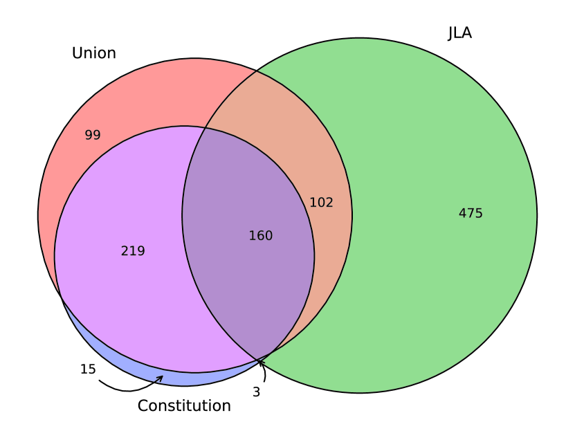
Figure 1: Venn diagram of the three SNe Ia catalogs. Overlapped data points are shown as labeled numbers.

In this paper, we used three SNe Ia catalogs in our analysis: Union2.1, Constitution, and JLA. Union2.1 includes 580 SNe Ia Suzuki2012 . The catalog covers samples with redshift range $0.015\leq z\leq 1.414$. Constitution catalog combines samples from Union and CfA3, containing 397 SNe Ia with redshifts in the range $0.015\leq z\leq 1.55$ Hicken2009 . The coordinate information of the Constitution catalog is adopted from the Open Supernova Catalog in this paper Guillochon2016 . JLA catalog includes several low-redshift samples ($z<0.1)$, all three seasons from the SDSS-II ($0.05<z<0.4$), and three years from SNLS ($0.2<z<1$). It includes 740 SNe Ia with high-quality light curves Betoule2014 . It covers redshift range $0.01\leq 1.30$. The three SNe Ia catalogs have some overlap in samples. The numbers of overlapped data points are shown in Figure 1.

2.2 Dipole fitting method

Firstly, we briefly introduce the dipole fitting method. For Union2.1 and Constitution data sets, the luminosity distance could be expanded by Hubble series parameters: Hubble parameter $H$, deceleration parameter $q$, jerk parameter $j$ and snap parameter $s$. These parameters can be expressed as functions of the scale factor $a$ and its derivatives,

$$H =\frac{\dot{a}}{a} q =-\frac{1}{H^{2}}\frac{\ddot{a}}{a}$$ (1)

$$j =\frac{1}{H^{3}}\frac{\dddot{a}}{a} s =\frac{1}{H^{4}}\frac{\ddddot{a}}{a}.$$

Taylor expansion of luminosity distance could be made in terms of redshift and Hubble series parameters Visser2004 . However, this expansion diverges at $z>1$. Thus, another parameter $y=z/(1+z)$ is introduced to overcome this problem. The luminosity distance can be expanded as a function of $y$ Cattoen2007 ; Wang2009

$$d_{\mathrm{L}}(y) =\frac{c}{H_{0}}[y-\frac{1}{2}(q_{0}-3)y^{2}+\frac{1}{6}(11-5q_{0}-j_{0})y^{3}$$ (2)

$$+\frac{1}{24}(50-7j_{0}-26q_{0}+10q_{0}j_{0}+21q_{0}^{2}-15q_{0}^{3}+s_{0})y^{4}$$

$$+O(y^{5})].$$

The distance modulus is defined as

$$\mu_{\mathrm{th}}=5\log\frac{d_{\mathrm{L}}}{\mathrm{Mpc}}+25.$$ (3)

Then the $\chi^{2}$ can be calculated as

$$\chi^{2}(H_{0},q_{0},j_{0},s_{0})=\sum_{i}\frac{(\mu_{\mathrm{obs},i}-\mu_{\mathrm{th},i})^{2}}{\sigma_{i}^{2}},$$ (4)

where $\mu_{\mathrm{obs}}$ and $\sigma_{i}$ are observational values of distance moduli and their errors, respectively. The best-fitting values of parameters could be obtained by minimizing $\chi^{2}(H_{0},q_{0},j_{0},s_{0})$.

For the JLA sample, the observational values of distance moduli are not directly given. Therefore, we use the values obtained in the $\Lambda$CDM model to avoid fitting too many free parameters simultaneously. The theoretical luminosity distance in $\Lambda$CDM model can be expressed as

$$d_{\mathrm{L}}(z)=\frac{(1+z)c}{H_{0}}\int_{0}^{z}\frac{\mathrm{d}z^{\prime}}{\sqrt{\Omega_{\mathrm{m}}(1+z)^{3}+(1-\Omega_{\mathrm{m}})}}.$$ (5)

Union2.1 and Constitution data sets already give $\mu_{\mathrm{obs}}$ as a part of the released data. For JLA data set, $\mu_{\mathrm{obs}}$ can be derived from light curve parameters of SN Ia from Betoule2014

$$\mu_{\mathrm{obs}}=m_{\mathrm{B}}^{*}-(M_{\mathrm{B}}-\alpha\times X_{1}+\beta\times\mathcal{C}),$$ (6)

where $m_{\mathrm{B}}^{*}$ is the observed peak magnitude in the rest-frame of the B band, $X_{1}$ describes the time stretching of light-curve, $\mathcal{C}$ describes the supernova color at maximum brightness and $M_{\mathrm{B}}$ is the absolute B-band magnitude, which depends on the host galaxy properties. $\alpha,\beta$ are nuisance parameters. $M_{\mathrm{B}}$ can be fitted by a simple step function related to $M_{\mathrm{stellar}}$ Johansson2013 ,

$$M_{\mathrm{B}}=\left\{\begin{array}[]{ll}M_{\mathrm{B}}^{1}&M_{\mathrm{stellar}}<10^{10}M_{\odot}\\ M_{\mathrm{B}}^{1}+\Delta_{M}&M_{\mathrm{stellar}}\geqslant 10^{10}M_{\odot}.\\ \end{array}\right.$$ (7)

where $M_{\mathrm{B}}^{1}$ and $\Delta_{M}$ are nuisance parameters. $\boldsymbol{C}(\alpha,\beta)$ is the total covariance matrix, which can be obtained with JLA data. $\chi^{2}$ is defined as

$$\chi^{2}_{JLA}(\alpha,\beta,M_{\mathrm{B}}^{1},\Delta_{M},\Omega_{\mathrm{m}})=(\boldsymbol{\mu}_{\mathrm{obs}}-\boldsymbol{\mu}_{\mathrm{th}})^{{\dagger}}\boldsymbol{C}^{-1}(\boldsymbol{\mu}_{\mathrm{obs}}-\boldsymbol{\mu}_{\mathrm{th}}).$$ (8)

By minimizing $\chi^{2}_{JLA}$, all free parameters mentioned above can be fitted. Our best-fitting results are consistent with those of Betoule2014 .

To quantify the anisotropic deviations on luminosity distance, we define the distance moduli with dipole $\boldsymbol{A}$ and monopole $B$ as

$$\tilde{\mu}_{\mathrm{th}}=\mu_{\mathrm{th}}(1-\boldsymbol{A}\cdot\hat{\boldsymbol{n}}+B),$$ (9)

where $\tilde{\mu}_{\mathrm{th}}$ is the theoretical value of distance modulus with dipolar direction dependence, and $\hat{\boldsymbol{n}}$ is the unit vector pointing at the corresponding SN Ia. $\boldsymbol{A}\cdot\hat{\boldsymbol{n}}$ represents the projected dipole magnitude in the direction of the given SNe Ia sample. $\hat{\boldsymbol{n}}$ can be represented in galactic coordinate as

$$\hat{\boldsymbol{n}}=\cos(b)\cos(l)\hat{\boldsymbol{i}}+\cos(b)\sin(l)\hat{\boldsymbol{j}}+\sin(b)\hat{\boldsymbol{k}}.$$ (10)

Then the projection is

$$\boldsymbol{A}\cdot\hat{\boldsymbol{n}}=\cos(b)\cos(l)A_{x}+\cos(b)\sin(l)A_{y}+\sin(b)A_{z}.$$ (11)

The best-fitting dipole and monopole parameters can be derived with the following steps:

1. Substitute $\mu_{\mathrm{th}}$ with $\tilde{\mu}_{\mathrm{th}}$ in the expression of $\chi^{2}$ as is shown in equation (4) and equation (8).

2. Fit the dipole $(A_{x},A_{y},A_{z})$ and the monopole component $B$ by minimizing $\chi^{2}$.

3. Transform the fitted dipole from Cartesian coordinate $(A_{x},A_{y},A_{z})$ back to spherical coordinate $(l,b,A)$.

Finally, we analyze the likelihood of the fitted parameters and the significance of dipole magnitude utilizing Markov Chain Monte Carlo (MCMC) sampling. To obtain the significance of dipole anisotropy precisely, we use the Monte Carlo simulation method Mariano2012 ; Yang2013 ; Wang2014 . To be specific, we construct a type of synthetic samples based on original data sets by assuming that theoretical values of distance moduli are “real” values. We refer to these synthetic samples as “isotropic” samples. Applying MCMC sampling on these samples, probability distributions of the fitted parameters can be obtained. They are also used to probe the effect of anisotropic factors, which we will discuss in section 4.

2.3 Quadrupole fitting

To examine whether a higher order of anisotropy exists, we fit the quadrupole along with the dipole in a similar manner as mentioned previously. We define the quadrupole $\mathbf{Q}$ in

$$\tilde{\mu}_{\mathrm{th}}=\mu_{\mathrm{th}}(1-\mathbf{Q}^{T}\hat{\boldsymbol{n}}\mathbf{Q}-\boldsymbol{A}\cdot\hat{\boldsymbol{n}}+B),$$ (12)

where $\mathbf{Q}$ is a symmetric, traceless $3\times 3$ matrix determined by 5 individual parameters.

2.4 Hemisphere comparison method

We applied hemisphere comparison method to the three samples. For a randomly chosen axis, data points contained in each hemisphere is used to fit $\Omega_{\mathrm{m}}$ individually, then the difference between each hemisphere is shown as

$$\delta=\frac{\Delta\Omega_{\mathrm{m0}}}{\bar{\Omega}_{\mathrm{m0}}}=\frac{\Omega_{\mathrm{m0,u}}-\Omega_{\mathrm{m0,d}}}{(\Omega_{\mathrm{m0,u}}+\Omega_{\mathrm{m0,d}})/2},$$ (13)

where the subscripts $u$ and $d$ represent the best parameter fitting value in the ‘up’ and ‘down’ hemispheres, respectively.

3 Results

3.1 Dipole fitting method

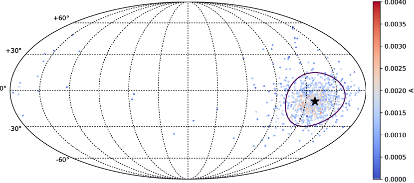
Figure 2: Best-fitting dipole direction (star) and 1$\sigma$ error range of the Union2.1 data set. Scatter points represent dipole fitting results of simulating samples.

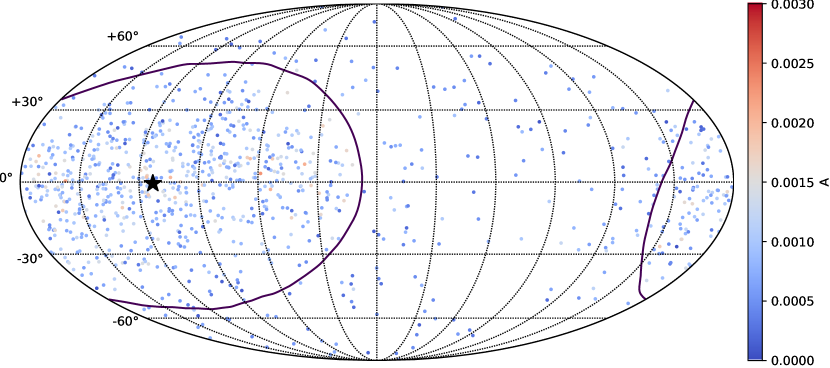
Figure 3: Similar to Figure 2 for the Constitution data set.

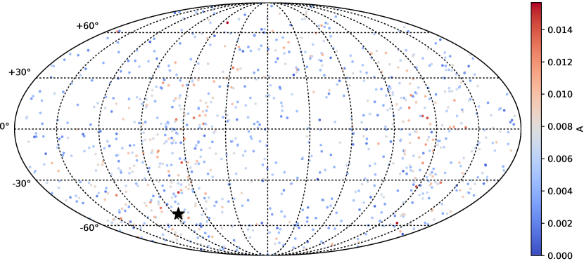
Figure 4: Best-fitting dipole direction (star) of the JLA data set. Scatter points represent dipole directions and magnitudes generated by MCMC sampling of original samples.

Fitting results are shown in Table 2. The confidence level is defined as the probability $\mathrm{P(|\boldsymbol{A}_{iso}|<|\boldsymbol{A}_{fit}|)}$, where $\mathrm{|\boldsymbol{A}_{iso}|}$ is the dipole magnitude of an arbitrary data set in “isotropic” samples, and $\mathrm{|\boldsymbol{A}_{fit}|}$ is the best-fitting dipole magnitude. Best-fitting dipole directions and 1$\sigma$ errors for Union2.1, Constitution, and JLA data sets, along with dipole fitting results of samples are plotted in Figures 2, 3 and 4, respectively.

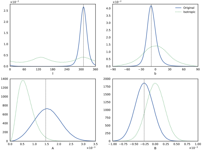
Figure 5: Blue lines show marginalized likelihoods of dipole $A$, monopole $B$ and $(l,b)$ for Union2.1 data set, and black vertical lines represent best-fitting values. Green dotted lines represent results of “isotropic” samples.

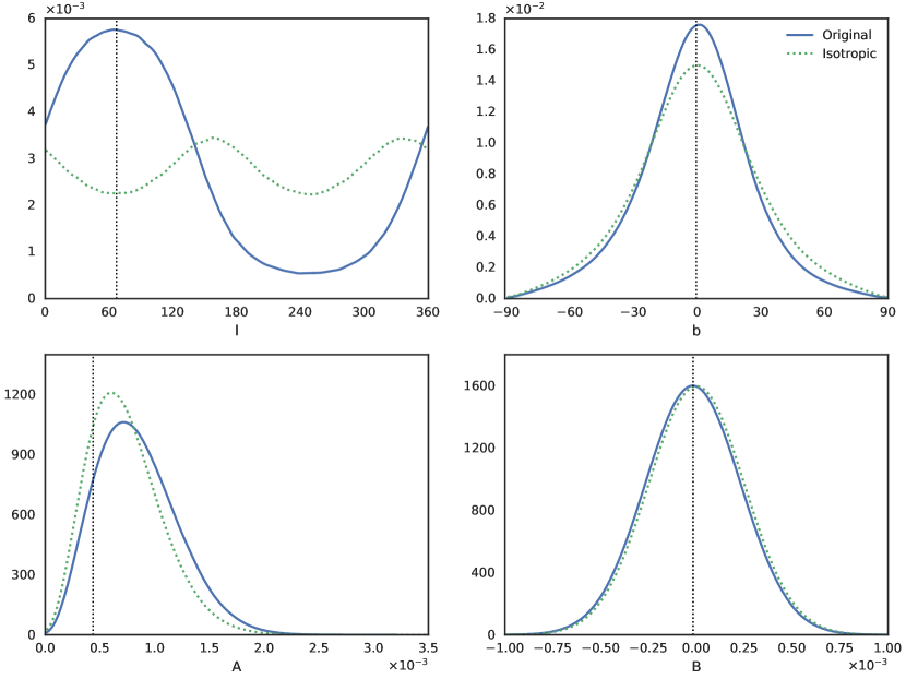
Figure 6: Similar to Figure 5 for Constitution data set.

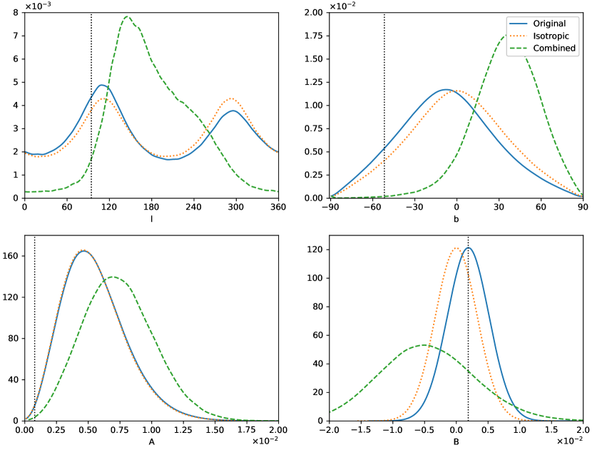
Figure 7: Blue lines show marginalized likelihoods of dipole $A$, monopole $B$ and $(l,b)$ for JLA data set, and black vertical lines represent best-fitting values. Orange dotted lines represent results of “isotropic” samples. Green dashed lines represent results of combined fitting of dipole parameters and nuisance parameters.

We generate $2\times 10^{6}$ effective samples for each data set for MCMC sampling. Probability distributions of dipole and monopole parameters for Union2.1, Constitution, and JLA data sets are shown in Figures 5, 6 and 7, respectively. Note that the best-fitting parameters do not coincide with most probable values for some parameters. This is because that the best-fitting values represent the maximum point of probability density function (PDF), while the most probable values in presented figures are the maximum values of marginal PDF of $l,b,A$, respectively. The marginalization process ”flattens” lots of information about the original PDF, thus the maxima can differ from those of the original PDF. Also notice that because the volume of parameter space approaches to zero when $A\to 0$ or $b\to\pm 90^{\circ}$, $A$ will always have zero likelihood at $A=0$ while having its maximum likelihood at some finite value, and $b$ will form a sine curve, even when samples are uniformly distributed around the origin. This does not affect the validity of analyzing the magnitude and direction of the dipole, so long as the sampling results are compared with those of “isotropic” samples, where deviations from “isotropic” scenario can be discerned from bias introduced from features of the spherical coordinate.

For Union2.1 data set, the direction and magnitude of the dipole are $(l=309.3^{\circ}{}^{+15.5^{\circ}}_{-15.7^{\circ}},\ b=-8.9^{\circ}{}^{+11.2^{\circ}}_{-9.8^{\circ}})$, and $\ A=(1.46\pm 0.56)\times 10^{-3}$. The confidence level of dipolar anisotropy is 98.3%. For Constitution data set, these parameters are $(l=67.0^{\circ}{}^{+66.5^{\circ}}_{-66.2^{\circ}},\ b=-0.6^{\circ}{}^{+25.2^{\circ}}_{-26.3^{\circ}})$, $\ A=(4.4\pm 5.0)\times 10^{-4}$, and $\ B=(-0.2\pm 2.4)\times 10^{-4}$. The confidence level of dipolar anisotropy is 19.7%.

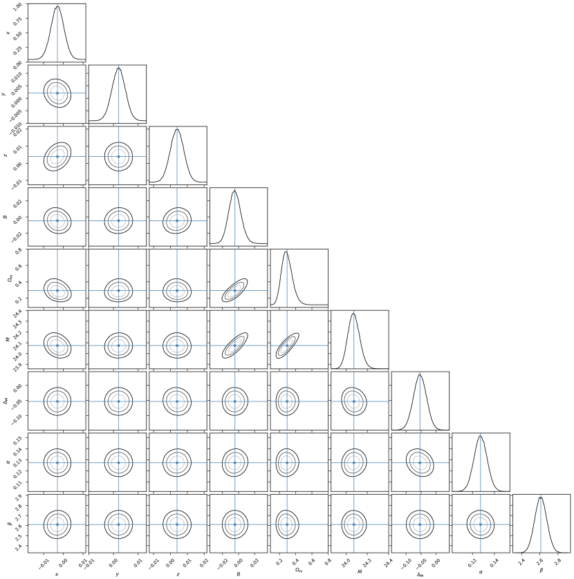
Figure 8: Probability distribution functions of dipole parameters and nuisance parameters when fitted simultaneously for JLA data set.

We fit JLA data set in two different approaches. Firstly, we fit nuisance parameters, then fit dipole parameters using the fitted nuisance parameters as constant. Secondly, we fit the nuisance parameters and dipole parameters simultaneously. Since nuisance parameters are related to both theoretical and observational values of distance moduli, “isotropic” synthetic data sets are not implemented in this approach. As is shown in Table 3, the combined fitting approach gives larger anisotropy than the separate fitting approach. Furthermore, the fitted values of nuisance parameters are slightly shifted. As shown in Figure 8, $B$, $\Omega_{\mathrm{m}}$, and $M$ are correlated.

It is worth mentioning that, JLA data set gives null results in dipole fitting. The 1$\sigma$ error range of dipole direction covers the whole celestial sphere. The confidence level of dipole magnitude is merely 0.23%. Furthermore, there is no significant difference between the likelihood of simulation results in 1$\sigma$ error range and full results. The same is true for the likelihood of parameters of “isotropic” samples and original samples. Besides, significant deviations exist in best-fitting values and most probable values of fitted parameters. Thus, no significant dipolar anisotropy of redshift-distance modulus relation is found in the JLA data set.

For Union2.1 data set, we get similar results as previous works Antoniou2010 ; Cai2012 ; Cai2013 ; Mariano2012 ; Yang2013 ; Wang2014 ; Lin2016 . For Constitution data sets, our results are different from those of Kalus2013 . Considering different methods, and the weak signal of the dipole in this data set, the difference is reasonable.

For JLA data set, we get different likelihood distributions as Lin2015 , which can be attributed to different fitting parameters used in the MCMC estimation. In this paper, we fit the dipole by fitting its rectangular components $(A_{x},A_{y},A_{z})$, then convert the fitting results to spherical coordinate. However, Lin2015 used the galactic coordinate $(l,b)$ and dipole magnitude $A$ directly. The likelihood distributions given in Lin2015 are inappropriate because the marginalized likelihood of $b$ does not approach zero at $b=\pm 90^{\circ}$. Moreover, the marginalized likelihood of $l$ at $0^{\circ}$ diverges from the likelihood at $360^{\circ}$, which is contrary to the fact that the two longitudes actually “wrap up” on the sphere. We also notice that some other work, such as Chang2018 ; Deng2018a ; Deng2018b shows similar improper likelihood distribution.

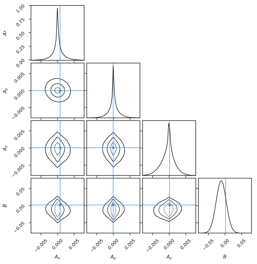
Figure 9: Probability distribution functions of rectangular components of dipole $\boldsymbol{A}$ and monopole $B$ for JLA data set directly using $(l,b,A)$ as fitted parameters.

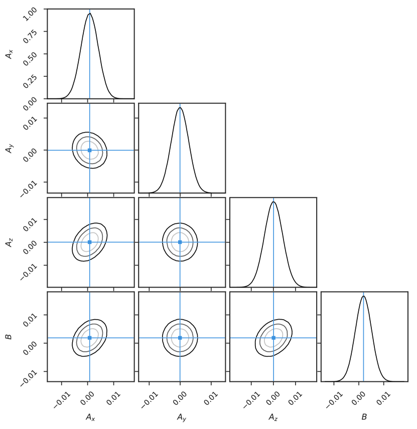
Figure 10: Probability distribution functions of rectangular components of dipole $\boldsymbol{A}$ and monopole $B$ for JLA data set directly using $(A_{x},A_{y},A_{z})$ as fitted parameters.

We fit parameter$(l,b,A)$ with constraints $0^{\circ}<l<360^{\circ},-90^{\circ}<b<90^{\circ},A>0$ enforced on them, i.e., sampling results out of such boundaries will be discarded by the MCMC sampler. By using the fitting method described above, the likelihood distributions mentioned in Lin2015 can be reproduced. Though seemingly proper, such constraints ignore the periodicity and symmetry of spherical coordinate, which results in artificial “gaps” on fitting parameters, thus blocking the sampler from properly sampling on those boundaries. As shown in Figure 9, non-zero likelihood at $b=\pm 90^{\circ}$ forms an unreasonable ‘spike’ at poles, which depends on the choice of the coordinate system. The proper method would be “set free” $(l,b,A)$ when sampling, then “wrap around” those parameters to their boundaries afterward. By using this “wrap around” technique, we reproduce the same posteriors as using rectangular components $(A_{x},A_{y},A_{z})$ for fitting. By comparison, posteriors used in this paper are following best-fitting values, and joint likelihood contours are smooth oval shapes, as shown in Figure 10.

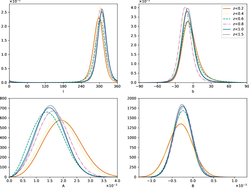
Figure 11: Marginalized likelihoods of dipole $A$, monopole $B$ and $(l,b)$ for different redshift range of Union2.1 data set.

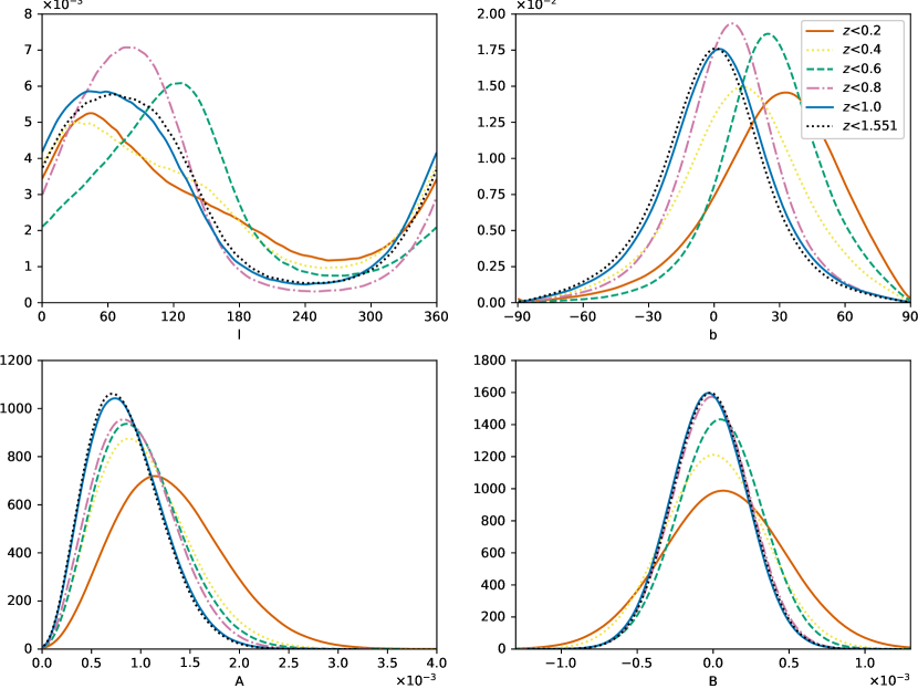
Figure 12: Similar to Figure 11, but for Constitution data set.

The redshift tomography results for Union2.1 and Constitution data sets are shown in Tables 4 and 5, respectively. The probability distributions for each data set are shown in Figures 11 and 12. Because the covariance matrix is involved in the fitting, it takes considerably long time to give the results for JLA sample, we do not perform the redshift tomography analysis.

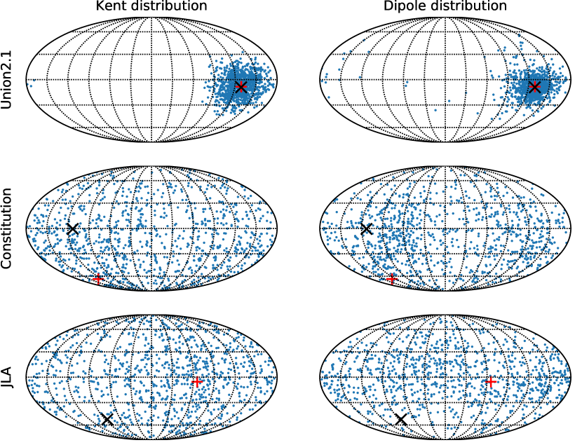
Figure 13: Left column shows samples drawn from fitted Kent distribution, the right column shows original dipole positions. Black x-cross shows the center of Kent distribution. Red cruciform shows the position of the best-fitting dipole.

We fit the spherical distribution of dipole position with Kent distributionKent1982 , which is the analogy to the bivariate normal distribution on the two-dimensional unit sphere. The samples drawn from Kent distribution are shown along with the original dipole positions in Figure 13. We find that Kent distribution fits well with dipole positions derived from Union2.1 data set, but is less suitable for Constitution and JLA data set.

3.2 Quadrupole fitting method

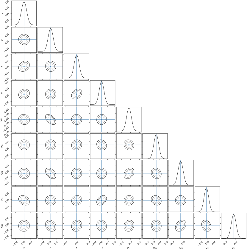
Figure 14: Probability distribution functions of dipole and quadrupole parameters.

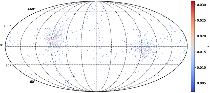
Figure 15: Distribution of eigenvectors with maximum eigenvalues of fitted quadrupole matrices, with eigenvalues represented in different colors.

We performed the quadrupole fitting method for the JLA data set. Five independent parameters $Q_{11},Q_{22},Q_{12},\allowbreak Q_{13},Q_{23}$ are used to represent the quadrupole $\mathbf{Q}$. The likelihood distributions of these parameters are shown in Figure 14. The distributions of the main eigenvectors are shown in Figure 15. The averaged absolute value of the determinant of fitted matrices is $4.1\times 10^{-7}$. The quadrupole of JLA data set is not significant.

3.3 Hemisphere comparison method

The hemisphere comparison results in different redshift bins are shown in Tables 6 and 7. The results are roughly following dipole fitting results for Union2.1 data set but show larger discrepancies for Constitution data set.

4 Discussions

4.1 Effects of anisotropy in data distribution

As shown in Figures 5, 6 and 7, even if no redshift-distance anisotropy in the input data, fitting results are still distributed an-isotropically (green dotted lines). This indicates other reasons, such as anisotropic coordinate or redshift distribution would affect the results.

To determine whether the coordinate distribution of samples would affect the results, we introduce two types of synthetic data sets.

Type A data sets

substituting the coordinates in the original data set with random coordinates uniformly distributed in the whole sky. $\boldsymbol{\mu}_{\mathrm{obs}}$ are replaced with synthetic data.

Type B data sets

substituting the coordinates in the original data set with random coordinates, but only uniformly distributed in the eastern hemisphere of the celestial sphere. Distance moduli are substituted in the same manner as type A data sets.

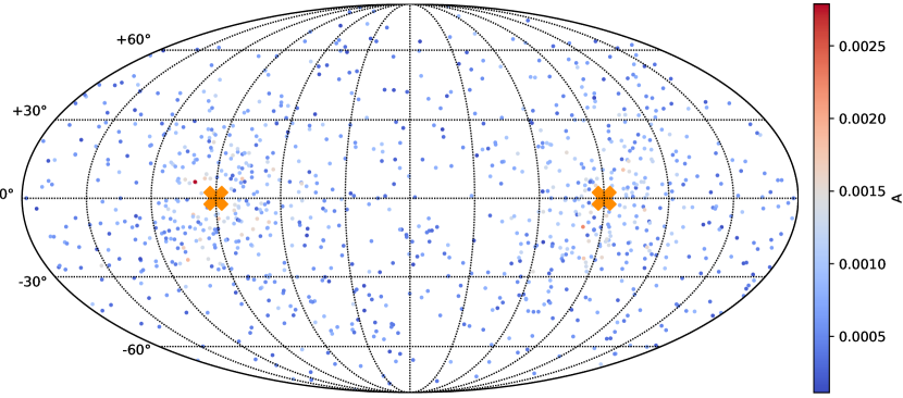
Figure 16: Distribution of dipole directions of type B samples. Dipole directions concentrate near crossed positions.

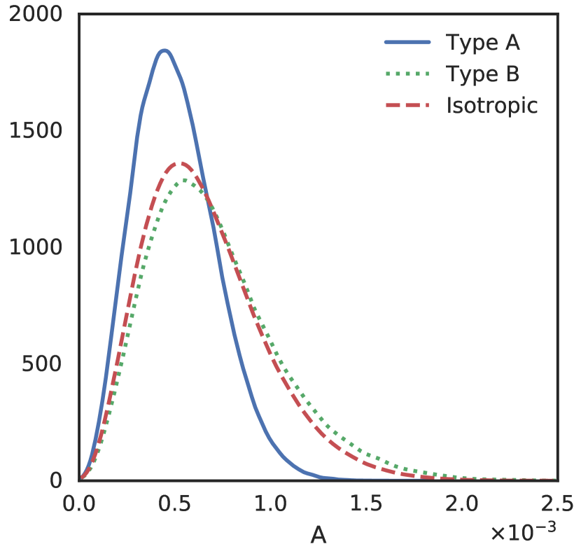
Figure 17: Likelihood of dipole magnitude $A$ of different samples. Blue solid line indicates the result of synthetic samples with isotropically distributed coordinates, which tend to reduce the dipole magnitude. Green dotted line indicates the result of synthetic samples with extremely an-isotropically distributed coordinates, which increase the dipole magnitude.

Using MCMC sampling method introduced in section 2, we find the dipoles in type A data sets are uniformly distributed in the whole sky. However, the dipoles in Type B data sets tend to concentrate in $(l,b)=(90^{\circ},0^{\circ})$, $(l,b)=(270^{\circ},0^{\circ})$, as shown in Figure 16. Meanwhile, dipole magnitudes are generally larger than it is in Type A data sets, as shown in Figure 17. This indicates that the anisotropy of coordinates of samples does affect the results of dipole fitting.

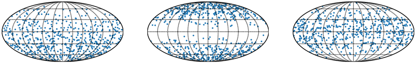
Figure 18: Coordinates generated for three synthetic data sets. The probability density functions of the coordinate density are proportional to $1-\sin(b)$, $\sin^{2}(b)$ and $\cos^{2}(b)$, respectively.

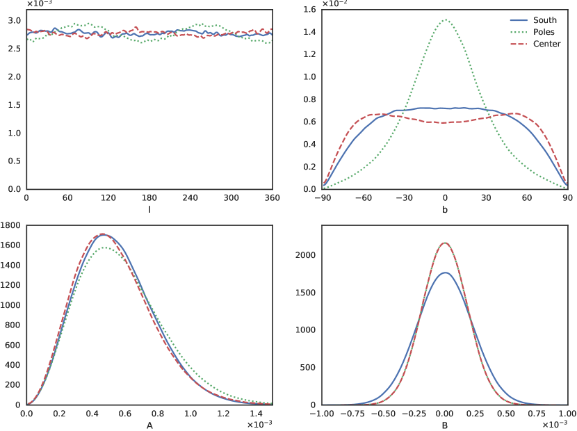
Figure 19: Probability distributions of three synthetic data sets with a specific coordinate distribution.

In addition, we generate three kinds of synthetic data sets with specific coordinate distributions, based on the Union2.1 data set. The probability density function of the randomly-generated coordinates are proportional to $1-\sin(b)$, $\sin^{2}(b)$ and $\cos^{2}(b)$, respectively. In other words, the coordinates are concentrated on the south galactic pole, both galactic poles, and the galactic plane, respectively, as is shown in Figure 18. Distance moduli are replaced in the same manner as “isotropic” data sets. The fitted results are shown in Figure 19.

The spatial distribution of redshifts can be anisotropic, i.e., the redshift of samples in one patch of the sky may be generally smaller than another patch of sky. This may also cause an influence on fitting results. To extract the effects of anisotropy in redshift distribution from other factors, we introduce another kind of synthetic data set.

Type C data sets

shuffle the coordinates in the original data set, making distance-related data of every sample correspond with a coordinate of another random sample in the data set. Keep the ‘shuffled coordinates’ order unchanged, then substitute distance moduli as type A data sets.

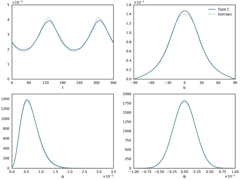
Figure 20: Likelihood of parameters for type C samples and isotropic samples. No significant deviation caused by the different spatial distribution of redshifts is found.

Using the generating method described above, we can alternate the spatial distribution of redshifts without changing the distribution of coordinates. We find that the fitting results of type C data sets are fairly consistent with “isotropic” samples, as shown in Figure 20. Therefore, the anisotropy of redshift distribution does not cause a significant influence on fitting results.

5 Conclusions

In this paper, we study three different data sets of SNe Ia, namely Union2.1, Constitution, and JLA, to find possible dipolar anisotropy in redshift-distance relation. We fit the dipole and monopole parameters by minimizing $\chi^{2}$, then run MCMC sampling to determine the error range and confidence level of the fitting parameters. We also apply the hemisphere comparison method to find possible anisotropy in $\Omega_{\mathrm{m}}$ on Union2.1 and Constitution data sets, and compare the results with dipole fitting method.

For Union2.1 data set, we find the direction and magnitude of the dipole are $(l=309.3^{\circ}{}^{+15.5^{\circ}}_{-15.7^{\circ}},\ b=-8.9^{\circ}{}^{+11.2^{\circ}}_{-9.8^{\circ}}),\ A=(1.46\pm 0.56)\times 10^{-3}$. The monopole magnitude is $B=(-2.6\pm 2.1)\times 10^{-4}$. The confidence level of dipolar anisotropy is 98.3%. Hemisphere comparison method gives $\delta=0.20,l=352^{\circ},b=-9^{\circ}$. For Constitution data set, these parameters are $(l=67.0^{\circ}{}^{+66.5^{\circ}}_{-66.2^{\circ}},\ b=-0.6^{\circ}{}^{+25.2^{\circ}}_{-26.3^{\circ}}),\ A=(4.4\pm 5.0)\times 10^{-4},\ B=(-0.2\pm 2.4)\times 10^{-4}$, The confidence level of dipolar anisotropy is 19.7%. The results of hemisphere comparison method are$\delta=0.56,l=141^{\circ},b=-11^{\circ}$. For JLA data set, fitted parameters are $l=94.4^{\circ},\ b=-51.7^{\circ},\ A=7.8\times 10^{-4},\ B=1.9\times 10^{-3}$. The 1$\sigma$ error range of dipole direction covers almost the whole sky. The confidence level of dipolar anisotropy is merely 0.23%. Redshift tomography results show slightly larger anisotropy at lower redshift range.

As shown above, the Union2.1 and Constitution data sets, although have a large portion of overlapped data points, give radically different results in terms of the best-fitting dipole parameters and confidence levels. Furthermore, JLA data set, which contains more data and a smaller portion of overlapped data than the other two data sets, gives an essentially null result in dipolar anisotropy. Due to the large discrepancies of the best-fitting dipole parameters among different data sets, and the low confidence level given by Constitution and JLA data set, we conclude that no sufficient evidence of dipolar anisotropy is found in the aforementioned three SNe Ia catalogs. The larger confidence level of dipolar anisotropy shown in Union2.1 data set may come from non-cosmological factors.

We also study the effects of anisotropy of coordinate and redshift distribution in dipole fitting method and find that anisotropy distribution of coordinates can cause dipole magnitude to become larger. However, anisotropy distribution of redshifts does not have a significant influence on fitting results.

In future, the next-generation cosmological surveys, such as LSST LSST2019 , Euclid Euclid2018 , and WFIRST WFIRST2018 will observe much larger SNe Ia data sets with enhanced light-curve calibration, which may shed light on the anisotropy in redshift-distance relation.

Table 1: Incomplete list of previous works on cosmological preferred directions. AM is short for a specific anisotropic model, DF for dipole fitting method, and HC for hemisphere comparison method.

Authors	Sample Used	Method	$(l,b)$	Anisotropy Level	C.L.
Antoniou & Perivolaropoulos (2010)Antoniou2010	Union2	HC	$(306^{\circ},15^{\circ})$	$\Delta\Omega_{m}/\Omega_{m}=0.42$	70%
Cai & Tuo (2012)Cai2012	Union2	HC	$(314^{\circ}{}^{+20^{\circ}}_{-13^{\circ}},28^{\circ}{}^{+11^{\circ}}_{-33^{\circ}})$	$\Delta q_{0}/q_{0}=0.79{}^{+0.27}_{-0.28}$
Cai et al. (2013)Cai2013	Union2+67GRB	AM	$(306^{\circ},-13^{\circ})$	$g_{0}=0.030{}^{+0.010}_{-0.030}$	2$\sigma$
Mariano & Perivolaropoulos (2012)Mariano2012	Union2	DF	$(309.4^{\circ}\pm 18.0^{\circ},-15.1^{\circ}\pm 11.5^{\circ})$	$A=(1.3\pm 0.6)\times 10^{-3}$	2$\sigma$
	Keck+VLT	DF	$(320.5^{\circ}\pm 11.8^{\circ},-11.7^{\circ}\pm 7.5^{\circ})$	$A=(1.02\pm 0.25)\times 10^{-5}$	3.9 $\sigma$
Kalus et al. (2013)Kalus2013	Constitution	HC	$(-35^{\circ},-19^{\circ})$	$\Delta H/H\sim 0.026$	95%
Yang et al. (2013)Yang2013	Union2.1	HC	No Significance	No Significance
		DF	$(307.1^{\circ}\pm 16.2^{\circ},-14.3^{\circ}\pm 10.1^{\circ})$	$A=(1.2\pm 0.5)\times 10^{-3}$	95.45%
Wang & Wang (2014)Wang2014	Union2.1+116GRB	DF	$(309.2^{\circ}\pm 15.8^{\circ},-8.6^{\circ}\pm 10.5^{\circ})$	$A=(1.37\pm 0.57)\times 10^{-3}$	97.29%
Lin et al. (2015)Lin2015	JLA	DF	No Significance	No Significance
Lin et al. (2016)Lin2016	Union2.1	HC	$(241.9^{\circ},-19.5^{\circ})$	$\Delta\Omega_{m}/\Omega_{m}=0.306$	37%
		AM	$(310,6^{\circ}\pm 18.2^{\circ},-13.0^{\circ}\pm 11.1^{\circ})$	$D=(1.2\pm 0.5)\times 10^{-3}$	95.9%
Deng & Wei (2018a)Deng2018a	JLA	DP	$(309.4^{\circ}\pm 18.0^{\circ},-15.1^{\circ}\pm 11.5^{\circ})$	$A=(1.3\pm 0.6)\times 10^{-3}$	2$\sigma$
		HC	$(23^{\circ},2^{\circ})\&(299^{\circ},28^{\circ})$	$\Delta\Omega_{m}/\Omega_{m}=0.31,0.28$
Deng & Wei (2018b)Deng2018b	Pantheon	DF	No Significance	No Significance
		HC	$(138^{\circ},-7^{\circ})\&(102^{\circ},-29^{\circ})$	$\Delta\Omega_{m}/\Omega_{m}=0.30,0.24$
Sun & Wang (2018)Sun2018	Pantheon	DF	$(108^{\circ}{}^{+43^{\circ}}_{-77^{\circ}},7^{\circ}{}^{+41^{\circ}}_{-77^{\circ}})$	$A=(2.6\pm 2.6)\times 10^{-4}$	36.2%
		HC	$(110^{\circ}\pm 11^{\circ},15^{\circ}\pm 19^{\circ})$	$\Delta\Omega_{m}/\Omega_{m}=0.105$

Table 2: Best-fitting results of dipole and monopole for three data sets. The confidence level (C.L.) is defined as the probability of the case where the dipole magnitude of an arbitrary data set in “isotropic” samples being smaller than the best-fitting dipole magnitude.

data sets	Union 2.1	Constitution	JLA
$l$	$309.3^{\circ}{}^{+15.5^{\circ}}_{-15.7^{\circ}}$	$67.0^{\circ}{}^{+66.5^{\circ}}_{-66.2^{\circ}}$	$94.4^{\circ}$
$b$	$-8.9^{\circ}{}^{+11.2^{\circ}}_{-9.8^{\circ}}$	$-0.6^{\circ}{}^{+25.2^{\circ}}_{-26.3^{\circ}}$	$-51.7^{\circ}$
$A$	$(1.46\pm 0.56)\times 10^{-3}$	$(4.4\pm 5.0)\times 10^{-4}$	$7.8\times 10^{-4}$
$B$	$(-2.6\pm 2.1)\times 10^{-4}$	$(-0.2\pm 2.4)\times 10^{-4}$	$1.9\times 10^{-3}$
C.L.	98.3%	19.7%	0.23%

Table 3: Fitted parameters of JLA data set for separated fitting and combined fitting.

Fitting method	$l$	$b$	$A$	$B$	$M_{\mathrm{B}}^{1}$	$\Delta_{M}$	$\alpha$	$\beta$	$\Omega_{\mathrm{m}}$
Separated	$94.4^{\circ}$	$-51.7^{\circ}$	$7.8\times 10^{-4}$	$1.9\times 10^{-3}$	24.12	-0.06	0.140	3.12	0.29
Combined	$171.7^{\circ}$	$48.2^{\circ}$	$5.3\times 10^{-3}$	$-4.6\times 10^{-3}$	24.07	-0.05	0.127	2.61	0.29

Table 4: Redshift tomography results for the Union2.1 data set using dipole fitting method.

$z$ range	$l$	$b$	$A$	$B$
$z<0.2$	$296.9^{\circ}$	$-6.3^{\circ}$	$1.8\times 10^{-3}$	$-3.0\times 10^{-4}$
$z<0.4$	$301.2^{\circ}$	$-11.0^{\circ}$	$1.8\times 10^{-3}$	$-3.1\times 10^{-4}$
$z<0.6$	$302.2^{\circ}$	$-8.1^{\circ}$	$1.3\times 10^{-3}$	$-2.4\times 10^{-4}$
$z<0.8$	$304.8^{\circ}$	$-13.5^{\circ}$	$1.6\times 10^{-3}$	$-2.3\times 10^{-4}$
$z<1.0$	$308.5^{\circ}$	$-9.7^{\circ}$	$1.4\times 10^{-3}$	$-2.5\times 10^{-4}$
$z<1.5$	$309.4^{\circ}$	$-8.9^{\circ}$	$1.5\times 10^{-3}$	$-2.6\times 10^{-4}$

Table 5: Similar to Table 4, but for the Constitution data set.

$z$ range	$l$	$b$	$A$	$B$
$z<0.2$	$64.1^{\circ}$	$54.5^{\circ}$	$6.9\times 10^{-4}$	$7.1\times 10^{-5}$
$z<0.4$	$65.4^{\circ}$	$28.3^{\circ}$	$4.2\times 10^{-4}$	$6.9\times 10^{-6}$
$z<0.6$	$106.0^{\circ}$	$41.9^{\circ}$	$5.9\times 10^{-4}$	$4.6\times 10^{-5}$
$z<0.8$	$73.3^{\circ}$	$10.6^{\circ}$	$5.9\times 10^{-4}$	$-1.2\times 10^{-5}$
$z<1.0$	$59.9^{\circ}$	$3.1^{\circ}$	$4.5\times 10^{-4}$	$-2.8\times 10^{-5}$
$z<1.55$	$67.0^{\circ}$	$-0.6^{\circ}$	$4.4\times 10^{-4}$	$-1.8\times 10^{-5}$

Table 6: Redshift tomography results using hemisphere comparison method for the Union2.1 data set.

$z$ range	$\delta$	$l$	$b$
$z\leq 0.2$	0.88	$306^{\circ}$	$-20^{\circ}$
$z\leq 0.4$	0.52	$325^{\circ}$	$15^{\circ}$
$z\leq 0.6$	0.20	$242^{\circ}$	$-47^{\circ}$
$z\leq 0.8$	0.22	$310^{\circ}$	$-30^{\circ}$
$z\leq 1.0$	0.20	$1^{\circ}$	$-3^{\circ}$
$z\leq 1.5$	0.20	$352^{\circ}$	$-9^{\circ}$

Table 7: Similar to Table 6, but for the Constitution data set.

Redshift range	$\delta$	$l$	$b$
$z\leq 0.6$	0.78	$141^{\circ}$	$-19^{\circ}$
$z\leq 0.8$	0.52	$31.6^{\circ}$	$-15^{\circ}$
$z\leq 1.0$	0.51	$135^{\circ}$	$-5^{\circ}$
$z\leq 1.0$	0.51	$135^{\circ}$	$-5^{\circ}$
$z\leq 1.55$	0.56	$126^{\circ}$	$-11^{\circ}$

References

- (1) M.M. Phillips, Astron. J. 413, L105 (1993)
- (2) A.G. Riess, et al., Astron. J. 116(3), 1009 (1998)
- (3) S. Perlmutter, et al., Astrophys. J. 517(2), 565 (1999)
- (4) P. Kroupa, M. Pawlowski, M. Milgrom, Int. J. Mod. Phys. D 21, 1230003 (2012)
- (5) P. Kroupa, Publ. Astron. Soc. Aust. 29(4), 395 (2012)
- (6) L. Perivolaropoulos, Galaxies 2(1), 22 (2014)
- (7) K. Koyama, Reports Prog. Phys. 79, 46902 (2016)
- (8) P. Vielva, et al., Astrophys. J. 609(1), 22 (2004)
- (9) A. de Oliveira-Costa, et al., Phys. Rev. D 69(6), 63516 (2004)
- (10) M. Tegmark, A. De Oliveira-Costa, A.J.S. Hamilton, Phys. Rev. D 68(12) (2003)
- (11) D. Hutsemékers, et al., Astron. Astrophys. 441(3), 915 (2005)
- (12) M.J. Longo, arXiv 04, 1 (2009)
- (13) J.A. King, et al., Mon. Not. R. Astron. Soc. 422(4), 3370 (2012)
- (14) A. Mariano, L. Perivolaropoulos, Phys. Rev. D 86(8) (2012)
- (15) Campanelli, L, et al., Phys. Rev. D 83(10) (2011)
- (16) X. Li, et al., Eur. Phys. J. C 73, 2653 (2013)
- (17) Y.Y. Wang, F.Y. Wang, Mon. Not. R. Astron. Soc. 474(3), 3516 (2018)
- (18) P.K. Aluri, et al., J. Cosmol. Astropart. Phys. 12(1), 3 (2013)
- (19) Z. Chang, et al., Eur. Phys. J. C 74, 2821 (2014)
- (20) I. Antoniou, L. Perivolaropoulos, J. Cosmol. Astropart. Phys. 12, 12 (2010)
- (21) R.G. Cai, Z.L. Tuo, J. Cosmol. Astropart. Phys. 2012, 6 (2012)
- (22) R.G. Cai, et al., Phys. Rev. D 87(12), 123522 (2013)
- (23) W. Zhao, P. Wu, Y. Zhang, Int. J. Mod. Phys. D 22, 1350060 (2013)
- (24) X. Yang, F.Y. Wang, Z. Chu, Mon. Not. R. Astron. Soc. 437(2), 1840 (2013)
- (25) J.S. Wang, F.Y. Wang, Mon. Not. R. Astron. Soc. 443(2), 1680 (2014)
- (26) B. Javanmardi, et al., Astrophys. J. 810(1), 47 (2015)
- (27) J.B. Jimenez, V. Salzano, R. Lazkoz, Phys. Lett. B 741, 168 (2015)
- (28) H.N. Lin, X. Li, Z. Chang, Mon. Not. R. Astron. Soc. 460(1), 617 (2016)
- (29) Z. Chang, et al., Mon. Not. R. Astron. Soc. 478, 3633 (2018)
- (30) H.K. Deng, H. Wei, Eur. Phys. J. C 78, 755 (2018)
- (31) H.K. Deng, H. Wei, Phys. Rev. D 97, 123515 (2018)
- (32) Z.Q. Sun, F.Y. Wang, Mon. Not. R. Astron. Soc. 478, 5153 (2018)
- (33) C. Bonvin, R. Durrer, M. Kunz, Phys. Rev. Lett. 96(19), 191302 (2006)
- (34) D.J. Schwarz, B. Weinhorst, Astron. Astrophys. 474(3), 717 (2007)
- (35) C. Gordon, K. Land, A. Slosar, Mon. Not. R. Astron. Soc. 387(1), 371 (2008)
- (36) J. Colin, et al., Mon. Not. R. Astron. Soc. 414(1), 264 (2011)
- (37) S. Turnbull, et al., Mon. Not. R. Astron. Soc. 420, 447 (2012)
- (38) B. Kalus, et al., Astron. Astrophys. 553(120824), 56 (2013)
- (39) S. Appleby, A. Shafieloo, J. Cosmol. Astropart. Phys. 10, 70 (2014)
- (40) D. Huterer, D. Shafer, F. Schmidt, J. Cosmol. Astropart. Phys. 12, 33 (2015)
- (41) R.G. Cai, et al., Phys. Rev. D 97, 103005 (2018)
- (42) P. Astier, et al., Astron. Astrophys. 447(1), 31 (2006)
- (43) M. Sullivan, et al., Astrophys. J. 737(2), 102 (2011)
- (44) J.A. Holtzman, et al., Astron. J. 136(6), 2306 (2008)
- (45) A. Rest, et al., Astrophys. J. 795(1), 44 (2014)
- (46) D.M. Scolnic, et al., Astrophys. J. 780(1), 37 (2014)
- (47) J.L. Tonry, et al., Astrophys. J. 750(2), 99 (2012)
- (48) M. Hicken, et al., Astrophys. J. 700(2), 1097 (2009)
- (49) M. Stritzinger, et al., Astron. J. 142(5) (2011)
- (50) G. Folatelli, et al., Astron. J. 139(1), 120 (2009)
- (51) C. Contreras, et al., Astron. J. 139(2), 519 (2009)
- (52) M. Ganeshalingam, W. Li, A.V. Filippenko, Mon. Not. R. Astron. Soc. 433(3), 2240 (2013)
- (53) G. Aldering, et al., in Proc. SPIE, vol. 4836, ed. by J.A. Tyson, S. Wolff (2002), vol. 4836, pp. 61–72
- (54) D. Rubin, et al., Astrophys. J. 695(1), 391 (2009)
- (55) H. Campbell, et al., Astrophys. J. 763(2), 88 (2013)
- (56) A. Conley, et al., Astrophys. Journal, Suppl. 192(1), 1 (2011)
- (57) N. Suzuki, et al., Astrophys. J. 746(1), 85 (2012)
- (58) M. Betoule, et al., Astron. Astrophys. 568, A22 (2014)
- (59) Guillochon, James, et al., Astrophys. J. 835(1) (2016)
- (60) M. Visser, Class. Quantum Gravity 21(11), 2603 (2004)
- (61) C. Cattoën, M. Visser, Class. Quantum Gravity 24, 5985 (2007)
- (62) F.Y. Wang, Z.G. Dai, S. Qi, Astron. Astrophys. 507(1), 53 (2009)
- (63) J. Johansson, et al., Mon. Not. R. Astron. Soc. 435(2), 1680 (2013)
- (64) H.N. Lin, et al., Mon. Not. R. Astron. Soc. 456(2), 1881 (2015)
- (65) J.T. Kent, J. R. Stat. Soc. Ser. B 44(1), 71 (1982)
- (66) Ž. Ivezić, et al., Astrophys. J. 873, 111 (2019)
- (67) L. Amendola, et al., Living Rev. Relativ. 21, 2 (2018)
- (68) R. Hounsell, et al., Astrophys. J. 867, 23 (2018)