Holographic Reconstruction of Bubbles

Abstract

We discuss the holographic reconstruction of static thin bubble walls in BTZ black hole geometries. We consider two reconstruction prescriptions suggested in recent years: hole-ography and light-cone cuts, in the context of thin bubble walls, and comment on their applicability in the presence of non-trivial matter in the bulk. We find that while the light-cone cuts prescription goes through within its own limitations, the current hole-ographic approaches are inadequate to describe bubble spacetimes completely. Much like entanglement shadows found around BTZ black holes and conical defects in the bulk, we find that thin bubbles are accompanied by shadows of their own, which are regions of spacetime which are only partially probed by minimal geodesics. We speculate that such shadows might be a generic feature of the presence of matter in the bulk.

1 Introduction

Since the seminal work of Maldacena in 1997 Maldacena:1997re , holography has came to become one of the cornerstones of twenty-first century high energy physics. The so called “AdS/CFT duality” has found a multitude of applications in condensed matter physics, as it provides a probe for studying strongly coupled highly quantum phenomenon in field theories using their dual weakly coupled semi-classical gravity theories. These applications have been well explored in the literature; see e.g. Hartnoll:2009sz ; McGreevy:2009xe ; Gubser:2009md and references therein. The other direction of this duality can in turn be used to potentially understand some characteristics of quantum gravity — which continues to be one of the most profound puzzles in physics — by looking at the well understood weakly coupled field theories. Soon after the AdS/CFT conjecture was proposed, these ideas began to take shape under the name of bulk reconstruction Balasubramanian:1999ri ; Giddings:1999qu . Since then, there has been a tremendous amount of research towards reconstructing local bulk operators from the boundary CFT ones Hamilton:2006az ; Hamilton:2005ju ; Hamilton:2006fh ; Hamilton:2007wj ; Almheiri:2014lwa ; Swingle:2012wq ; Qi:2013caa . See DeJonckheere:2017qkk for an excellent set of lecture notes on the subject, and references therein.

An important part of the bulk reconstruction program is to understand how classical spacetime emerges from the underlying quantum degrees of freedom. Presumably, any theory of quantum gravity should provide an answer to this question, however, the precise mechanism is still unknown. In the holographic setting, one would like to isolate the degrees of freedom in the boundary field theory that might encode the information about the geometry, or more specifically the metric, of the bulk spacetime. A number of proposals have been put forth in this regard over the past two decades, perhaps the most developed of which is the idea that the bulk spacetime emerges from the entanglement structure of the boundary field theory Ryu:2006bv ; VanRaamsdonk:2009ar . In $(2+1)$ bulk dimensions, which will be the focus of this paper, these ideas have been rigorously developed using boundary observables like entanglement entropy, differential entropy and entwinement Balasubramanian:2013lsa ; Czech:2014ppa ; Myers:2014jia ; Headrick:2014eia ; Balasubramanian:2014sra ; Balasubramanian:2016xho . Another more recent approach to bulk reconstruction, called light-cone cuts, uses $n$-point correlation functions in the boundary field theory to obtain the bulk metric in arbitrary number of dimensions up to a conformal factor Engelhardt:2016wgb .

Most of the work cited above for geometric bulk reconstruction trials the methods with a fairly limited class of bulk geometries: global AdS₃, BTZ black holes and point conical defects, all of which are quotients of AdS₃. It is important therefore to subject these proposals to further tests, and in particular, to apply these recipes to more complicated (and hence realistic) geometries, which will allow us to understand them better and help determine their limits of applicability. To this end, in this paper we consider spacetimes with massive thin shells as an interesting candidate to test the validity of the proposed bulk reconstruction approaches. These spacetimes have several generic features related to the problem: the presence of non-trivial matter in the bulk in the form of a collapsing or expanding thin shell is combined with almost the same amount of isometries as in the empty AdS spacetime. However crucially, the presence of the shell-matter in the bulk causes a controllable breaking of the bulk symmetries that can lead to interesting features in the dual boundary field theory.

There are two type of physical processes which could be described by massive thin shells. A collapsing shell describes the process of a spherical collapse and black hole formation in AdS spacetime. This would correspond to a thermalisation process in the boundary field theory and has been explored e.g. in Danielsson:1999zt ; Danielsson:1999fa . Thin wall bubbles also describe the process of false vacuum decay Coleman:1977py ; Coleman:1980aw , can be time dependent or static, and can occur with or without a black hole Gregory:2013hja ; Burda:2015isa ; Burda:2015yfa . Aspects of their dual holographic description were studied in Barbon:2010gn . We will concentrate on the special case at the boundary of these two examples — static shells in $(2+1)$-dimensions. These can be viewed as special instantons in the context of vacuum decay, or as limits of flows or domain walls in AdS. The advantage of using a thin wall is that it is an analytic gravitational set-up. We can therefore derive analytic expressions for the quantities being proposed in bulk reconstruction, and easily explore their validity.

Our set-up is such that the static shell solution bounds two BTZ black hole spacetimes: the inside “$-$” and outside “$+$” respectively. These two spacetimes in general have different mass parameters, $M_{-}\neq M_{+}$, and different AdS radii, $\ell_{-}<\ell_{+}$. We refer to these spacetimes as BTZ bubbles, and it is clear that they cover a wide range of geometries, easily generalisable to higher dimensions. Leaving consideration of this, and dynamical shells, for the future, it is worth mentioning that time evolution of the holographic entanglement entropy in higher dimensions with collapsing shells has previously been studied in the adiabatic limit in Keranen:2015fqa . However, the question of bulk reconstruction was not addressed there.

We will focus on two proposals for bulk reconstruction in this paper that use a geometrical approach to the problem, in the sense that they define points and distances in the bulk via introduction of auxiliary geometric constructions on top of the boundary field theory data. The first approach was introduced in Balasubramanian:2013lsa ; Czech:2014ppa , which we will refer to as “hole-ography”. This method provides a recipe to reconstruct the spatial part of the bulk metric using the entanglement structure of the boundary CFT, which involves observables like entanglement entropy, differential entropy and entwinement. This proposal is quite natural, as the very first indication of an “emergence” of the bulk geometry was seen in the Ryu-Takayanagi formula for holographic entanglement entropy Ryu:2006bv . It has been widely felt that the entanglement entropy data of the boundary field theory should play an important role in bulk reconstruction, therefore, we discuss holographic entanglement entropy for the BTZ bubble spacetimes in details in section 3. The hole-ography method itself is reviewed and applied to BTZ bubble spacetimes in section 4.1.

The second and more recent approach of using light-cone cuts to reconstruct bulk geometry was introduced in Engelhardt:2016crc ; Engelhardt:2016wgb . This method provides a strategy to obtain the metric of the bulk spacetime up to an overall conformal factor. However, only the part of the spacetime that is in a casual contact with the boundary can be reconstructed using this prescription. The method is based on the knowledge of the divergence structure of the correlation functions in the boundary CFT. We will review this method in details in section 4.2 and provide explicit examples of the reconstruction of empty AdS, BTZ black hole and BTZ bubble spacetimes.

In addition to the comments on reconstructability of bubbles, we note the existence of what we call “bubble shadows”. These are a region of spacetime surrounding a bubble in the bulk, which can be seen as a particular generalisation of entanglement shadows discussed extensively in the literature (see e.g.  Balasubramanian:2014sra ; Freivogel:2014lja ; Balasubramanian:2017hgy ). Unlike an entanglement shadow however, which is a region of spacetime where minimal length geodesics (Ryu-Takayanagi surfaces) do not enter, these bubble shadows are only partially probed by minimal geodesics. Given that entanglement shadows have been found in BTZ black holes and spacetimes with a conical defect, which can be seen as point matter sources in the bulk, it seems to suggest that such shadows might be a generic feature of the presence of matter in the bulk.

The paper is structured as follows. We give an overview of static thin wall bubble geometries and their geodesics in section 2. In section 3 we give a detailed discussion of holographic entanglement entropy in the presence of bubbles in the bulk, and note the existence of bubble shadows. In section 4 we investigate hole-ographic and light-cone cuts reconstruction schemes in the context of bubble spacetimes. Finally, we close with discussion in section 5. In the appendix, we present the construction of kinematic spaces associated with bubble spacetimes.

2 Static bubble geometry

We will start with a brief review of thin wall bubbles and Israel junction conditions (see Gregory:2008rf for more details). We will work out various kinds of geodesics in this geometry, which will form the basis for our discussion in the bulk of this work. A generic bubble spacetime in arbitrary dimensions consists of an infinitesimally thin wall separating two bulk solutions of the vacuum Einstein’s equations. The symmetries of our setup and bubble wall energy-momentum require that each bulk has the form of an AdS black hole Bowcock:2000cq . The vacuum energy and mass parameters of the black hole on each side are, in general, different and related to the tension of the bubble wall via the Israel junction conditions Israel:1966rt . Generically, a bubble will have a time-dependent trajectory, however, to illustrate the issues in geometric bulk reconstruction, it is sufficient to consider the subset of bubble geometries that are static. We therefore briefly review the $(2+1)$-dimensional bubble geometries in this section before considering their holographic interpretation.

2.1 Static bubble metric

Recall that the metric of a $(2+1)$-dimensional BTZ black hole can be written as

$$ds^{2}=\frac{1}{z^{2}}\left(-\left(1-Mz^{2}\right)dt^{2}+dx^{2}+\frac{\ell^{2}}{1-Mz^{2}}dz^{2}\right),$$ (1)

with coordinates $t,x\in\mathbb{R}$ and $z\in(0,1/\sqrt{M})$. Here $\ell$ is the AdS radius related to the cosmological constant as $\Lambda=-1/\ell^{2}$ and $M$ is the mass parameter of the black hole. Notice that this metric is invariant under the scaling of coordinates $\{t,x,z\}\to\{\lambda t,\lambda x,\lambda z\}$ if we transform $M\rightarrow M/\lambda^{2}$. The horizon of the black hole is at $z=1/\sqrt{M}$, while $z\to 0$ represents the asymptotic boundary of the spacetime.

It is worth pointing out that our coordinate $x\in\mathbb{R}$, and hence the horizon of the black hole, is non-compact. This is in contrast with most of the holographic literature on this subject (see e.g. Ryu:2006bv ; Ryu:2006ef ), where $x\in\mathrm{S}^{1}$ is taken to be compact. An important feature of these compact black holes, as is well illustrated in Ryu:2006bv ; Ryu:2006ef , is that for any interval at the boundary, there is an infinite cascade of geodesics anchored at its end points, characterised by their winding number around the black hole. For a major part of this work, we will be interested in holographic entanglement entropy, wherein the length of the shortest among these infinite set of geodesics computes the entanglement entropy of the boundary interval in question, while the longer ones are said to compute “entwinement” Balasubramanian:2014sra . As we shall explore in the due course, the presence of a bubble gives rise to two new geodesics for some boundary intervals, on top of the infinite cascade arising due to compactness. Therefore by going to a non-compact version of the BTZ black hole, which is essentially an infinite cover of the compact one, we can efficiently isolate and focus on the effects of the bubble.

To construct a bubble spacetime, we will “glue” together two BTZ black holes with masses $M_{\pm}$ and AdS radii $\ell_{\pm}$ along a timelike hypersurface given by $z=Z(\tau)$, while respecting the translation invariance in $x$ direction. Here $\tau$ is a timelike coordinate on the hypersurface. The geometry is supported by a brane/bubble with constant tension $\sigma$ on the hypersurface. By a suitable choice of coordinates, we take an ansatz for the metric

$$ds^{2}=\begin{cases}\displaystyle\frac{1}{z^{2}}\left(-(1-M_{+}z^{2})dt^{2}_{+}+dx^{2}+\frac{\ell_{+}^{2}}{1-M_{+}z^{2}}dz^{2}\right)&\quad\text{for}\quad z\leq Z(\tau),\vspace{0.1cm}\\ \displaystyle\frac{1}{z^{2}}\left(-(1-M_{-}z^{2})dt^{2}_{-}+dx^{2}+\frac{\ell_{-}^{2}}{1-M_{-}z^{2}}dz^{2}\right)&\quad\text{for}\quad z\geq Z(\tau).\end{cases}$$ (2)

The bulk time coordinates are given by $t_{\pm}$, which becomes a function of $\tau$ in the vicinity of the bubble. For this ansatz to be consistent, it should induce the same metric on the bubble $z=Z(\tau)$ from either sides. If we represent the induced metric on the bubble as

$$ds^{2}_{\text{Bubble}}=h_{ij}dx^{i}dx^{j}=\frac{1}{{Z(\tau)}^{2}}\left(-d\tau^{2}+dx^{2}\right),$$ (3)

this gives a consistency condition on the bulk metric ansatz

$$(1-M_{\pm}Z^{2})\dot{t}^{2}_{\pm}-\frac{\ell_{\pm}^{2}\dot{Z}^{2}}{(1-M_{\pm}Z^{2})}=1,$$ (4)

where dot denotes the derivative with respect to $\tau$. This condition should be read as relating the time coordinates $t_{\pm}$ to $\tau$. In particular for a static bubble, defined by $\dot{Z}=\ddot{Z}=0$, this boils down to a simple relation

$$t_{+}\sqrt{1-M_{+}Z^{2}}=t_{-}\sqrt{1-M_{-}Z^{2}}=\tau.$$ (5)

Except on the bubble, metric in eq. 2 is merely a BTZ black hole and hence satisfies the Einstein equations. On the bubble however, Einstein equations imply that this geometry can be supported by a uniform tension bubble with an energy-momentum tensor $T^{i}_{\ j}=-\sigma\delta^{i}_{\ j}$, provided the Israel junction conditions Israel:1966rt are met

$$8\pi G\sigma =-\sqrt{\frac{1-M_{+}Z^{2}}{\ell_{+}^{2}}+\dot{Z}^{2}}+\sqrt{\frac{1-M_{-}Z^{2}}{\ell_{-}^{2}}+\dot{Z}^{2}},$$

$$\frac{\ddot{Z}-\frac{M_{+}Z}{\ell_{+}^{2}}}{\sqrt{\frac{1-M_{+}Z^{2}}{\ell_{+}^{2}}+\dot{Z}^{2}}} =\frac{\ddot{Z}-\frac{M_{-}Z}{\ell_{-}^{2}}}{\sqrt{\frac{1-M_{-}Z^{2}}{\ell_{-}^{2}}+\dot{Z}^{2}}}.$$ (6)

For the static case these conditions simplify considerably, and imply a range of parameter space where we are allowed to have a static bubble. For $M_{\pm}\neq 0$, section 2.1 in the static case implies

$$8\pi G\sigma=\sqrt{\left(\frac{M_{-}}{\ell_{-}^{2}}-\frac{M_{+}}{\ell_{+}^{2}}\right)\left(\frac{1}{M_{-}}-\frac{1}{M_{+}}\right)},\qquad Z=\frac{1}{\sqrt{M_{+}M_{-}}}\sqrt{\frac{\frac{M_{-}^{2}}{\ell_{-}^{2}}-\frac{M_{+}^{2}}{\ell_{+}^{2}}}{\frac{M_{-}}{\ell_{-}^{2}}-\frac{M_{+}}{\ell_{+}^{2}}}}.$$ (7)

Requiring the bubble tension $\sigma\geq 0$ and radius $0<Z<\min(\frac{1}{\sqrt{M_{+}}},\frac{1}{\sqrt{M_{-}}})$, it gives the allowed range of parameter space as

$$M_{+}\geq M_{-},\qquad\frac{\ell_{+}}{M_{+}}\geq\frac{\ell_{-}}{M_{-}},$$ (8)

which also implies a weaker condition $\ell_{+}\geq\ell_{-}$. On the other hand, if either of the black hole masses $M_{+}$ or $M_{-}$ is zero, the static condition forces the other mass to vanish as well. Consequently for $M_{\pm}=0$, using section 2.1 we get

$$8\pi G\sigma=\frac{1}{\ell_{-}}-\frac{1}{\ell_{+}},\qquad Z\in\mathbb{R}^{+},$$ (9)

with the allowed region of parameter space

$$\ell_{+}\geq\ell_{-}.$$ (10)

It is interesting to note that in both the cases, the bubble separates a BTZ spacetime with a less negative cosmological constant and higher mass parameter in the UV (near the boundary) from a more negative cosmological constant and lower mass parameter in the IR (deep in the bulk). This is in agreement with a holographic c-theorem Freedman:1999gp ; Myers:2010tj .

2.2 Spatial geodesics

During our discussion of bulk reconstruction later, we will extensively need the form of geodesics in the bulk. Hence we dedicate this subsection and the next to derive geodesics in static bubble geometries. The bubble spacetime is locally a BTZ black hole everywhere except in the vicinity of the bubble. So to find the geodesics we can use the following trick: we can start with the known geodesics in the “$+$” and “$-$” parts of the spacetime independently, and “glue” them with suitable boundary conditions (corresponding to the local continuity and smoothness of the geodesic). As innocuous as it sounds, this procedure can be quite cumbersome for a generic geodesic. Fortunately, for our purposes it suffices to consider just two special cases: spatial geodesics confined to a constant time slice and null geodesics that reach out to the boundary.

By a straightforward computation, one finds that spatial geodesics on a constant time slice of the BTZ metric in eq. 1 are given by two distinct branches. First kind of geodesics start from the boundary, turn at a point $(t_{0},x_{0},z_{0})$ in the bulk and return to the boundary:

$$t=t_{0},\qquad x=x_{0}\pm\frac{\ell}{\sqrt{M}}\sinh^{-1}\left(\sqrt{\frac{M(z_{0}^{2}-z^{2})}{1-Mz_{0}^{2}}}\right)\quad\text{with}\quad 0<z_{0}<\frac{1}{\sqrt{M}}.$$ (11)

These are the geodesics one would consider when computing entanglement entropy of a spatial slice at the boundary. The other kind of geodesics start from the boundary, cross the black hole horizon and escape all the way to the other asymptotic boundary:

$$t=t_{0},\qquad x=x_{0}\pm\frac{\ell}{\sqrt{M}}\cosh^{-1}\left(\sqrt{\frac{M(z_{0}^{2}-z^{2})}{Mz_{0}^{2}-1}}\right)\quad\text{with}\quad\frac{1}{\sqrt{M}}<z_{0}<\infty.$$ (12)

One would employ these if one needs to understand entanglement between the two asymptotic regions. If we are interested in the intervals at a boundary of the BTZ black hole, they are not quite as useful. However, upon introduction of bubbles, we find that they in fact start to play an important role.

For notational clarity, let us combine the two branches of geodesics into an analytically continued form

$$t=t_{0},\qquad x=x_{0}\pm\frac{\ell}{\sqrt{M}}\mathcal{S}^{-1}\left[z,z_{0},M\right]\,,$$ (13)

where

$${\cal{S}}^{-1}\left[z,z_{0},M\right]=\sinh^{-1}\left(\sqrt{\frac{M(z_{0}^{2}-z^{2})}{1-Mz_{0}^{2}}}\right)-\frac{i\pi missing}{2}\Theta({\textstyle|z_{0}|-\frac{1}{\sqrt{M}}}).$$ (14)

Here $0<z_{0}<\infty$ and $\Theta(z)$ is the Heaviside theta function. We have illustrated some representative geodesics in figure 1.

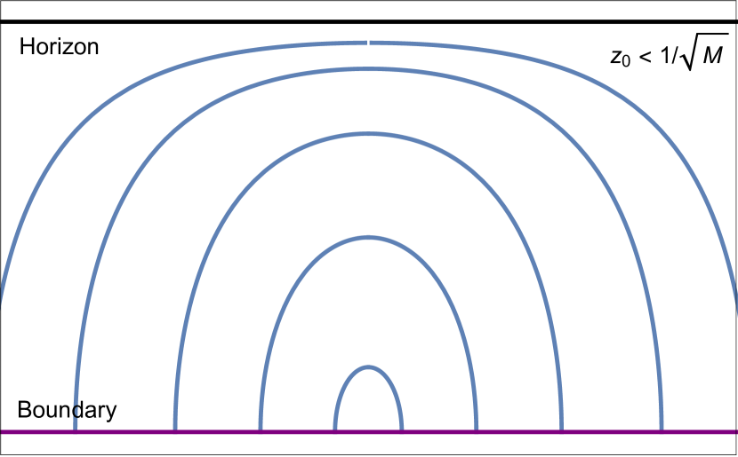
(a)

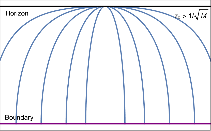
(b)

Figure 1: Spatial geodesics for BTZ black holes with (a) $0<z_{0}<1/\sqrt{M}$ and (b) $1/\sqrt{M}<z_{0}<\infty$. [Parameters: $\ell=1$, $M=0.1$, $t_{0}=0$ and $x_{0}=0$]. Note that the second branch of geodesics appears to be grazing the horizon and returning, but this is just a product of an inappropriate set of coordinates. They indeed cross the horizon, as can be illustrated by computing their slope at the horizon.

We construct spatial geodesics in the static bubble geometry by gluing spatial geodesics in the “$+$” and “$-$” spacetimes, given in eq. 13, and requiring continuity and smoothness of the geodesic on the bubble. If the geodesic turns at a point $(t_{0},x_{0},z_{0})$ in “$+$” spacetime with $z_{0}\leq Z$, it does not enter the “$-$” spacetime at all, and is simply given by

$$t_{+}=t_{0},\qquad x=x_{0}\pm\frac{\ell_{+}}{\sqrt{M_{+}}}{\cal{S}}^{-1}\left[z,z_{0},M_{+}\right]\,.$$ (15)

On the other hand if $z_{0}>Z$, then the geodesic will enter the minus spacetime, thus crossing the bubble at two distinct points. Although the spatial coordinates $x$ and $z$ have been chosen to be continuous across the bubble wall, the time coordinates are different on each side, so the time $t_{+}=t_{0}$ on the plus side of the bubble will match up to $t_{-}=\gamma t_{0}$ on the minus side, where $\gamma=\sqrt{\frac{1-M_{+}Z^{2}}{1-M_{-}Z^{2}}}$ is the time warp factor when we cross the wall. Once on the minus side of the bubble, the geodesic will have the standard form

$$t_{-}=\gamma t_{0}\;,\qquad x=x_{0}\pm\frac{\ell_{-}}{\sqrt{M_{-}}}\mathcal{S}^{-1}\left[z,z_{0},M_{-}\right],$$ (16)

that must be matched through the bubble to a generic geodesic segment in the plus spacetime

$$t_{+}=t_{0}\pm\alpha_{1}\;,\qquad x=x_{0}\pm\alpha_{2}\pm\frac{\ell_{+}}{\sqrt{M_{+}}}{\cal{S}}^{-1}\left[z,\alpha_{3},M_{+}\right].$$ (17)

The constants $\alpha_{1}$, $\alpha_{2}$ and $\alpha_{3}$ are fixed by local continuity and smoothness of the geodesic at the bubble

$$\alpha_{1}=0,\qquad\alpha_{2}=\frac{\ell_{-}}{\sqrt{M}_{-}}{\cal{S}}^{-1}\left[Z,z_{0},M_{-}\right]-\frac{\ell_{+}}{\sqrt{M}_{+}}{\cal{S}}^{-1}\left[Z,z_{0},M_{+}\right],\qquad\alpha_{3}=z_{0}.$$ (18)

These geodesics start from the boundary in “$+$” spacetime and reach the bubble, then (in this coordinate system) “refract” through the bubble to a standard “$-$” geodesic. Depending on how $z_{0}$ compares to $1/\sqrt{M_{-}}$, these geodesics will either turn and return via a similar trajectory, or will cross the horizon all the way to the other asymptotic boundary.

Note that the geodesics in bubble geometry only cross the horizon if $z_{0}>1/\sqrt{M_{-}}$. In particular if $M_{+}>M_{-}$, geodesics with $1/\sqrt{M_{+}}<z_{0}<1/\sqrt{M_{-}}$ will stay well away from the black hole. These geodesics have segments in the “$+$” spacetime which would have crossed the horizon by themselves in the absence of the bubble, but the bubble refracts them such that they do not make it to the horizon after all.

To summarize, spatial geodesics in bubble geometry are given in the “$+$” spacetime as

$$t_{+} =t_{0},$$ (19)

$$x =x_{0}\pm\frac{\ell_{+}}{\sqrt{M_{+}}}{\cal{S}}^{-1}\left[z,z_{0},M_{+}\right]$$

$$\qquad\pm\Theta({\textstyle z_{0}-Z})\left(\frac{\ell_{-}}{\sqrt{M_{-}}}{\cal{S}}^{-1}\left[Z,z_{0},M_{-}\right]-\frac{\ell_{+}}{\sqrt{M_{+}}}{\cal{S}}^{-1}\left[Z,z_{0},M_{+}\right]\right),$$

while for $z_{0}>Z$ they also have a branch in the “$-$” spacetime

$$t_{-}=\gamma t_{0},\qquad x=x_{0}\pm\frac{\ell_{-}}{\sqrt{M_{-}}}{\cal{S}}^{-1}\left[z,z_{0},M_{-}\right].$$ (20)

These different types of spatial bubble geodesics are shown in figure 2. As discussed in Balasubramanian:2011ur , the physical effect of the bubble and the interior BTZ spacetime is analogous to a medium with lower refractive index to the exterior BTZ geometry. Geodesics therefore have a tendency to cross to the interior “$-$” spacetime to transit across the bulk. This gives rise to interesting phenomena when considering the length of such geodesics, which we will review in section 3 while talking about holographic entanglement entropy.

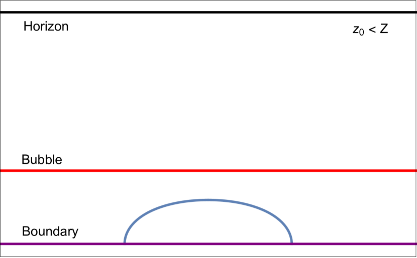
(a)

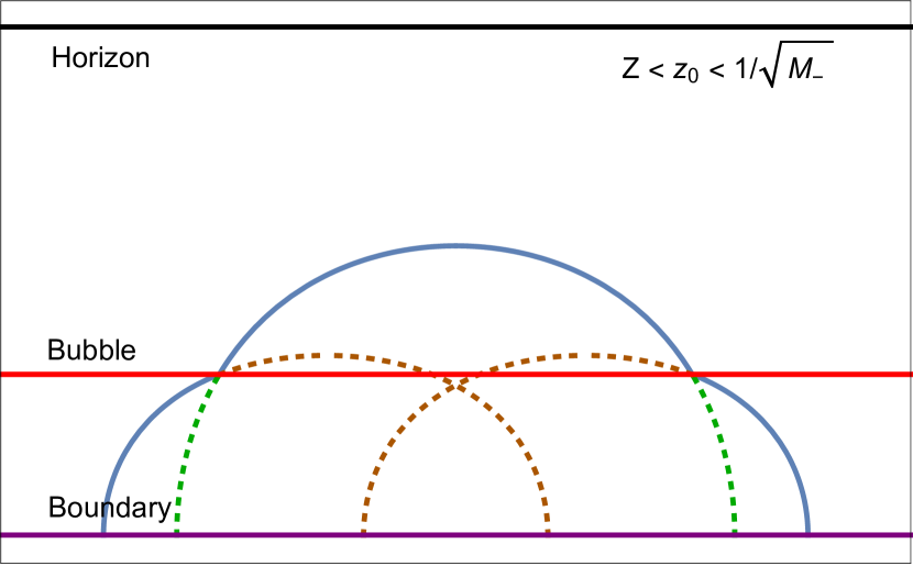
(b)

Figure 2: Sample spatial geodesics for BTZ bubbles for (a) $z_{0}<Z$ and (b) $Z<z_{0}<1/\sqrt{M_{-}}$. Dotted lines represent geodesics in “$+$” and “$-$” spacetimes, which have been “glued” together to get the resultant geodesics in bubble spacetime. [Parameters: $\ell_{+}=2$, $M_{+}=0.8$, $\ell_{-}=1$, $M_{-}=0.1$, $Z=1$, $t_{0}=0$, $x_{0}=0$ and $z_{0}=0.6,\leavevmode\nobreak\ 1.8$].

2.3 Null geodesics

We now move on to the discussion of null geodesics. A generic null geodesic for the BTZ black hole metric (1), which escapes to the boundary, is given as,

$$\begin{split}t&=t_{0}\pm\frac{\ell}{\sqrt{M}}\mathcal{T}_{t}^{-1}[z,p,M],\quad\mathcal{T}_{t}^{-1}[z,p,M]=\tanh^{-1}\left(\frac{z\sqrt{M}}{\sqrt{1-p^{2}(1-Mz^{2})}}\right),\\ x&=x_{0}\pm\frac{\ell}{\sqrt{M}}\mathcal{T}_{x}^{-1}[z,p,M],\quad\mathcal{T}_{x}^{-1}[z,p,M]=\tanh^{-1}\left(\frac{pz\sqrt{M}}{\sqrt{1-p^{2}(1-Mz^{2})}}\right).\end{split}$$ (21)

Here $(t_{0},x_{0})$ are coordinates of a point at the boundary where the geodesic hits, while $p\in(-1,1)$ represents the momentum of the null geodesic in $x$ direction. We can also find null geodesics which do not escape to the boundary, but we will not need them in this work.

Now performing an analysis similar to that for the spatial geodesics, i.e. considering null geodesics in “$+$” and “$-$” spacetimes and imposing suitable boundary conditions on the bubble, we can recover null geodesics for static BTZ bubbles. The resultant solutions for the ones that escape to the boundary are: for $z<Z$ in “$+$” spacetime

$$\begin{split}t_{+}&=t_{0}\pm\frac{\ell_{+}}{\sqrt{M_{+}}}\Big{(}\mathcal{T}_{t}^{-1}[z,p_{0},M_{+}]-\mathcal{T}_{t}^{-1}[Z,p_{0},M_{+}]\Big{)}\pm\frac{1}{\gamma missing}\frac{\ell_{-}}{\sqrt{M_{-}}}\mathcal{T}_{t}^{-1}[Z,\gamma p_{0},M_{-}],\\ x&=x_{0}\pm\frac{\ell_{+}}{\sqrt{M_{+}}}\Big{(}\mathcal{T}_{x}^{-1}[z,p_{0},M_{+}]-\mathcal{T}_{x}^{-1}[Z,p_{0},M_{+}]\Big{)}\pm\frac{\ell_{-}}{\sqrt{M_{-}}}\mathcal{T}_{x}^{-1}[Z,\gamma p_{0},M_{-}],\end{split}$$ (22)

and for $z\geq Z$ in “$-$” spacetime

$$t_{-}=\gamma t_{0}\pm\frac{\ell_{-}}{\sqrt{M}_{-}}\mathcal{T}_{t}^{-1}[z,\gamma p_{0},M_{-}],\qquad x=x_{0}\pm\frac{\ell_{-}}{\sqrt{M_{-}}}\mathcal{T}_{x}^{-1}[z,\gamma p_{0},M_{-}].$$ (23)

Here $(t_{0},x_{0})$ are coordinates of a point at the boundary where the geodesic hits, while $p_{0}$ and $\gamma p_{0}$ represent the momentum of the null geodesic in the $x$ direction in “$+$” and “$-$” spacetime respectively.

This finishes our general discussion of static bubble geometries. We constructed static uniform tension infinitesimally thin bubbles with a BTZ black hole geometry on either sides, and studied the behavior of some special geodesics in this spacetime. In the following sections we will use these results to probe some exciting holographic implications of these bubbles.

3 Holographic entanglement entropy

In recent years, there has been a tremendous amount of interest in connections between quantum gravity and quantum information theory. We have learned that we can get some profound insights into the quantum nature of gravity by appealing to techniques pertaining to quantum information Ryu:2006bv ; Lewkowycz:2013nqa ; Maldacena:2013xja ; Brown:2015bva . Perhaps the best understood of these insights come from a field theory observable called the “entanglement entropy”. Naively, entanglement entropy $S_{A}$ of a spatial region $A$ in a field theory is a measure of quantum entanglement between degrees of freedom living in $A$ and those in its complement. For an excellent review on the subject, see Rangamani:2016dms . For field theories which admit a holographic dual, entanglement entropy can be computed using the formula due to Ryu-Takayanagi Ryu:2006bv ; Hubeny:2007xt

$$S_{A}=\min_{i}\left(\frac{\text{Area}(\Sigma^{i}_{A})}{4G}\right).$$ (24)

Here $\Sigma^{i}_{A}$ are extremal area surfaces in the bulk anchored at $A$ at the boundary, i.e. $\partial\Sigma_{A}^{i}=\partial A$, and are homologous to $A$ (can be smoothly deformed into $A$ at the boundary). The index “$i$” runs over multiple such surfaces, if available, in which case the formula picks up the minimal area surface. For a $(1+1)$-dimensional field theory which has a $(2+1)$-dimensional bulk dual, like the ones we are interested in, spatial region $A$ is just an interval at the boundary and $\Sigma^{i}_{A}$ is a spacelike geodesic anchored at its end points.

We would like to use this framework of holographic entanglement entropy for our case of static bubble geometries. This would allow us to better understand the holographic interpretation of these bubbles. From the boundary field theory perspective, dynamics of thin bubble walls in a black hole spacetime is understood as a thermalisation process Balasubramanian:2011ur . It was noted in Balasubramanian:2011ur , for the case when $M_{-}=0$, that entanglement entropy in these dual field theories shows an interesting swallowtail behaviour. This is due to the presence of multiple spatial geodesics that are anchored at the same boundary interval. We will inspect this behaviour in detail in the following for arbitrary BTZ masses, focusing on the static limit. We will see later in section 4.1 that this swallowtail behaviour has important consequences for the holographic reconstruction of bubble spacetimes.

3.1 BTZ black holes

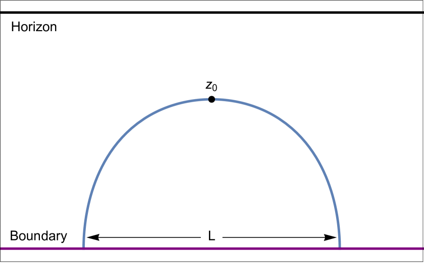
(a)

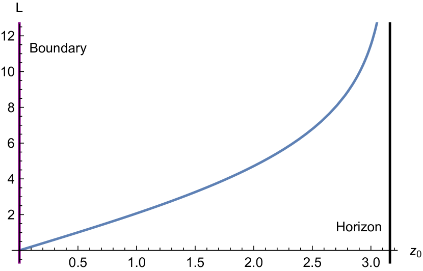
(b)

Figure 3: (a) Spatial geodesics anchored at a boundary interval of length $L$. (b) Length of the interval spanned at the boundary $L$ as a function of $z_{0}$. [Parameters: $\ell=1$, $M=0.1$, and in (a) $t_{0}=0$, $x_{0}=0$, $z_{0}=2$ and $L=4.71$].

Let us start with a warm-up exercise of computing holographic entanglement entropy in a bubble-free BTZ black hole spacetime. A detailed analysis can be found, for example, in Ryu:2006bv . Recall that the metric of a BTZ black hole is given by eq. 1. For an interval in the boundary with endpoints $(t_{0},x_{0}\pm L/2)$ at the boundary to be linked by a bulk spatial geodesic, we require

$$L=\frac{2\ell}{\sqrt{M}}{\cal{S}}^{-1}\left[0,z_{0},M\right],$$ (25)

where the parameter $z_{0}$ refers to the turning point of the geodesic in the bulk, which is in defined eq. 13. This constraint has is solved by

$$z_{0}=\frac{1}{\sqrt{M}}\tanh\left(\frac{\sqrt{M}}{\leavevmode\nobreak\ 2\ell}L\right).$$ (26)

See figure 3 for a diagrammatic representation. We can compute the length of this geodesics as

$$S_{\epsilon}=2\ell\log\left(\frac{2z_{0}/\epsilon missing}{\sqrt{1-Mz_{0}^{2}}}\right)+\mathcal{O}(\epsilon)=2\ell\log\left(\frac{2/\epsilon missing}{\sqrt{M}}\sinh\left(\frac{\sqrt{M}}{2\ell}L\right)\right)+\mathcal{O}(\epsilon),$$ (27)

where $\epsilon$ is an infinitesimal UV cut-off. It determines the entanglement entropy of the interval of length $L$ via the Ryu-Takayanagi formula:

$$S_{\mathrm{EE}}(L)=\frac{c}{3}\log\left(\frac{2\beta}{a}\sinh\left(\frac{L}{2\beta}\right)\right),$$ (28)

where $c=3\ell/2G$ is the central charge of the CFT, $a=\epsilon\ell$ is the length scale associated with the UV cutoff in the CFT and $\beta=\ell/\sqrt{M}$ is the inverse temperature. See figure 4 for a plot of $S$ verses the turning point $z_{0}$ and the boundary interval $L$.

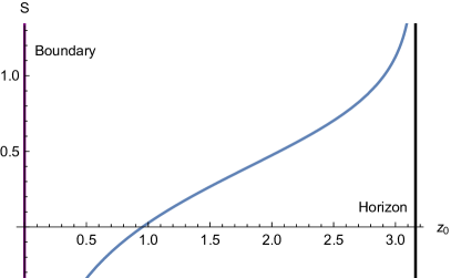
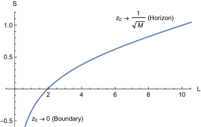
Figure 4: Renormalized holographic entanglement entropy for BTZ black holes. The first plot shows the behaviour of renormalized entangling function $S$ as a function of $z_{0}$, while the second shows the mutual behaviour of $S$ with $L$ for varying $z_{0}$. [Parameters: $\ell=1$, $M=0.1$, $G_{3}=1$].

3.2 Static BTZ bubbles

We can now move on to our primary case of interest: static BTZ bubble spacetimes. Eq. 19 implies that for a geodesic to be anchored at a boundary interval $(t_{0},x_{0}\pm L/2)$, we must have:

$$L=\frac{2\ell_{+}}{\sqrt{M_{+}}}\mathcal{S}^{-1}\left[0,z_{0},M_{+}\right]+\Theta({\textstyle z_{0}-Z})\left(\frac{2\ell_{-}}{\sqrt{M_{-}}}\mathcal{S}^{-1}\left[Z,z_{0},M_{-}\right]-\frac{2\ell_{+}}{\sqrt{M_{+}}}\mathcal{S}^{-1}\left[Z,z_{0},M_{+}\right]\right).$$ (29)

Unlike the pure BTZ case however, this relation is not simply analytically invertible, apart from the case when $z_{0}<Z$. Nevertheless, we can qualitatively analyse the behaviour of $L$ as we increase $z_{0}$. The first term in eq. 29 is an increasing function of $z_{0}$ until the turning point $z_{0}=1/\sqrt{M_{+}}>Z$ is reached. At that point, the constraints on the parameters of the plus and minus geometries, eq. 8, imply that the second term in eq. 29 is negative. Specifically, expanding $z_{0}=Z+\delta z_{0}$ for small $\delta z_{0}$, we see that

$$L\approx\frac{2\ell_{+}}{\sqrt{M_{+}}}\mathcal{S}[0,Z,M_{+}]+\frac{2\ell_{+}\delta z_{0}}{1-M_{+}Z^{2}}+\Theta(\delta z_{0})\sqrt{8Z\delta z_{0}}\left(\frac{\ell_{-}}{\sqrt{1-M_{-}Z^{2}}}-\frac{\ell_{+}}{\sqrt{1-M_{+}Z^{2}}}\right),$$ (30)

and hence $L(z_{0})$ has a local maximum at $z_{0}=Z$. Meanwhile, as $z_{0}\to 1/\sqrt{M_{-}}$, $L\to\infty$, hence $L$ has a minimum between $Z$ and $1/\sqrt{M_{-}}$, while for $z_{0}>1/\sqrt{M_{-}}$, $L$ decreases again, approaching zero as $z_{0}\to\infty$. This behaviour is displayed in figure 5 for a sample set of parameters for the bubble geometry.

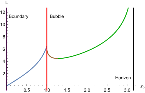
Figure 5: Length of the interval spanned at the boundary $L$ against the turning point $z_{0}$. [Parameters: $\ell_{+}=2$, $M_{+}=0.8$, $\ell_{-}=1$, $M_{-}=0.1$, $Z=1$].

We can tie this behaviour to the fact that there are now three distinct types of spatial geodesics, depending on the value of $L$. For small $L$, i.e.

$$L<L_{a}=\frac{2\ell_{+}}{\sqrt{M_{+}}}\tanh^{-1}\left(\sqrt{M_{+}}Z\right)\,,$$ (31)

there are ‘branch (a)’ geodesics, remaining entirely within the “$+$” spacetime. As we increase the interval length past some $L=L_{c}<L_{a}$, two new branches of geodesics pop-up, as it becomes preferable for the geodesic to cross the bubble wall and take a path through the “$-$” spacetime. (see the middle plot in figure 6). One of these new geodesics, called ‘branch (c)’ goes deeper in the bulk than the other, called ‘branch (b)’. These geodesics will persist until $L=L_{a}$, at which point it is no longer possible for a geodesic to remain in the plus spacetime, and we will simply have a ‘branch (c)’ geodesic. See the third plot in figure 6). Figure 6 shows these different branches of spatial geodesics as $L$ increases, and figure 5 shows a plot of the length of the geodesics as a function of $z_{0}$.

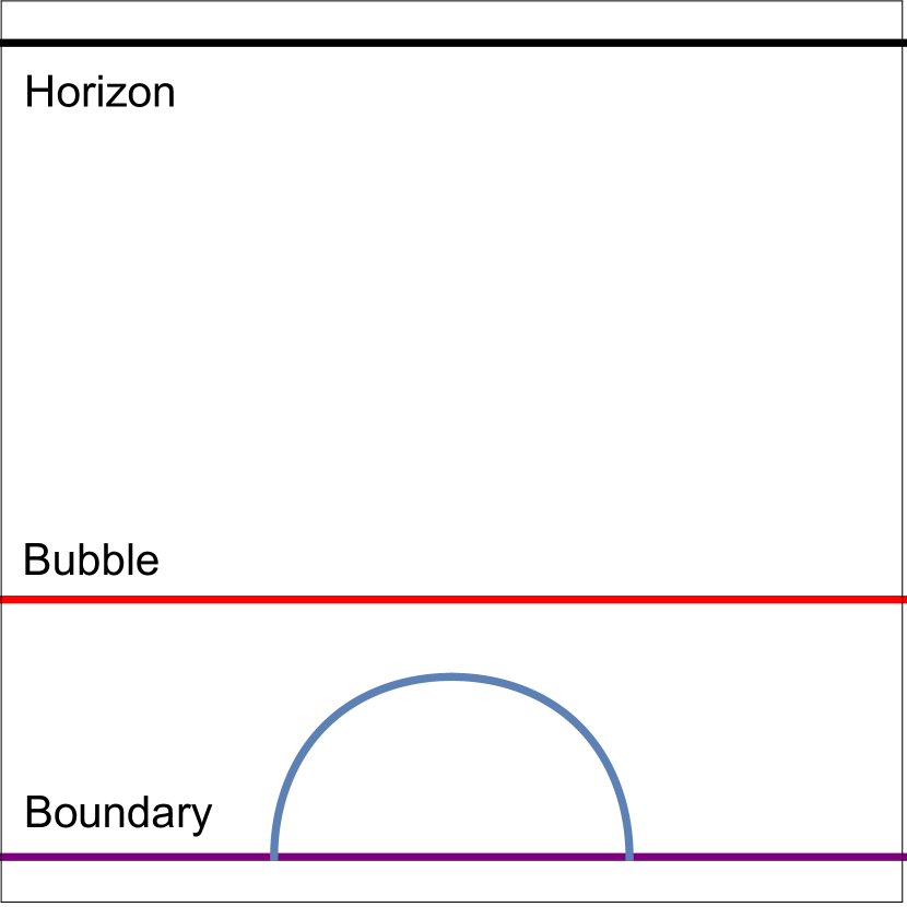
(a)

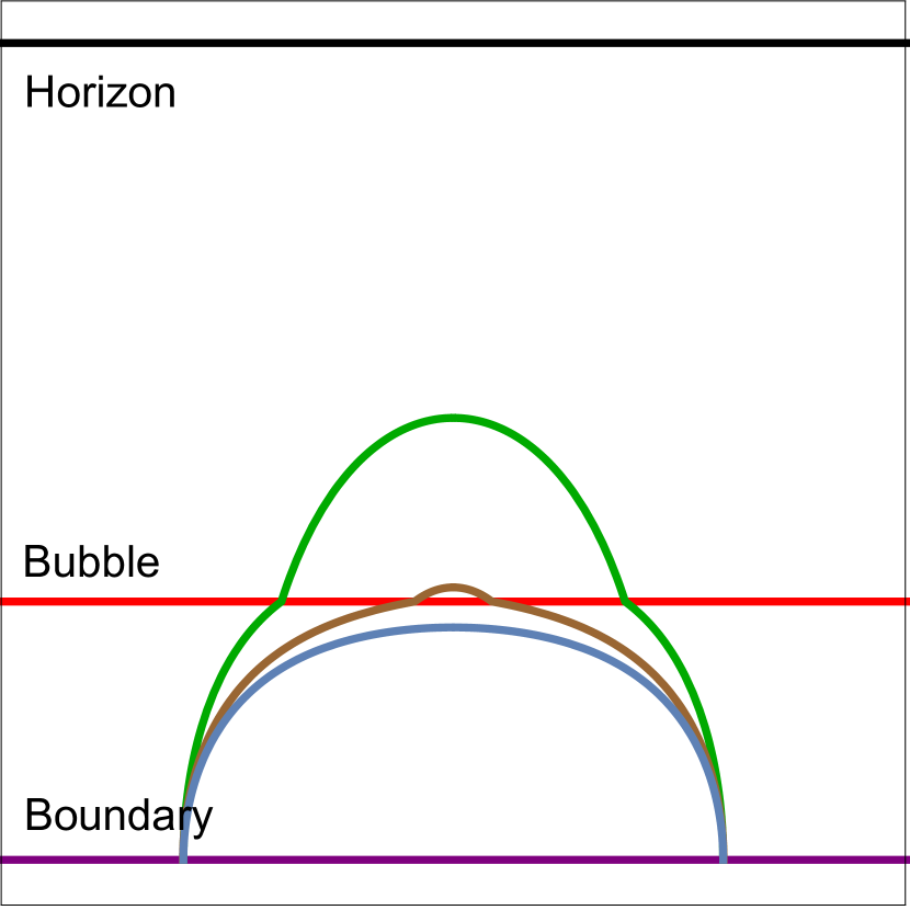
(b)

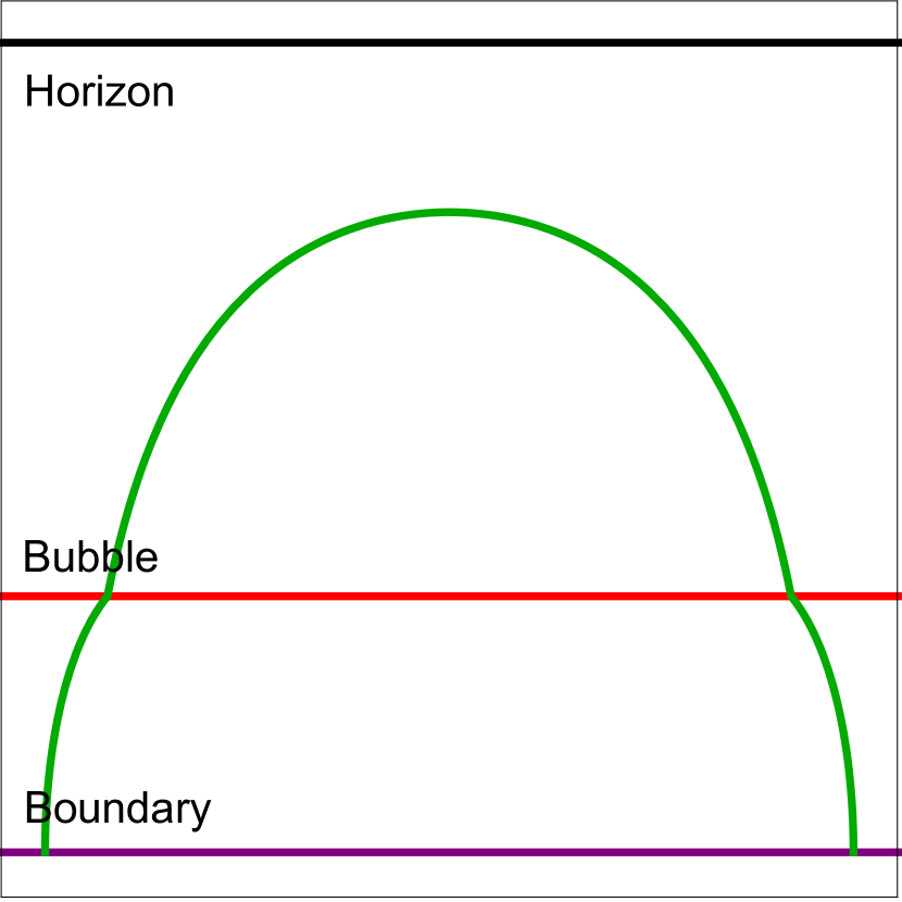
(c)

Figure 6: Multiple geodesics anchored at the boundary. The geometry parameters are: $\ell_{+}=2$, $M_{+}=0.8$, $\ell_{-}=1$, $M_{-}=0.1$, and $Z=1$. In plot (a) $L=2.15$, with $z_{0}=0.5$, in (b), $L=5.07$, with $z_{0}=0.9,\leavevmode\nobreak\ 1.05,\leavevmode\nobreak\ 1.71$, and in plot (c), $L=7.52$, with $z_{0}=2.5$.

The physical appearance of these geodesics suggests an interesting phase structure as we vary the boundary interval $L$. For small $L$, we expect the minimal length geodesic to remain ‘close’ to the boundary. However, as $L$ increases and the geodesic gets near to the bubble in the bulk, we might expect that it becomes preferable for the geodesic to ‘jump’ across the bubble wall, refracting into the interior “$-$” spacetime to cross the bulk at lower cost. To confirm this suspicion, we need to compare the length of these various geodesics. In terms of the parameter $z_{0}$, we find that the length of the geodesic has the form

$$S_{\epsilon} =2\ell_{+}\left[\log\left(\frac{2z_{0}/\epsilon missing}{\sqrt{1-M_{+}z_{0}^{2}}}\right)-\Theta(z_{0}-Z)\sinh^{-1}\left(\sqrt{\frac{Z^{-2}-z_{0}^{-2}}{z_{0}^{-2}-M_{+}}}\right)\right]$$

$$\qquad+2\Theta(z_{0}-Z)\ell_{-}\sinh^{-1}\left(\sqrt{\frac{Z^{-2}-z_{0}^{-2}}{z_{0}^{-2}-M_{-}}}\right).$$ (32)

Thus we can readily infer the geometric length of the spacelike geodesics connecting intervals of length $L$ on the boundary. In figure 7 we show the behaviour of the renormalized geodesic length $S=S_{\epsilon}+2\ell_{+}\log(\epsilon/2)$ as a function of $z_{0}$ and $L$. The geodesic with least length for a given value of the interval length $L$ determines the entanglement entropy for that interval, while the longer geodesics can be interpreted as determining entwinement Balasubramanian:2014sra .

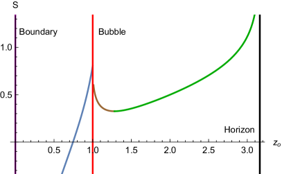
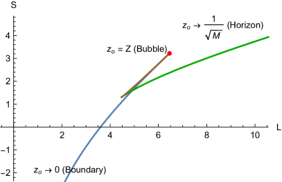
Figure 7: Renormalized holographic entanglement entropy for BTZ bubbles. The first plot shows the behaviour of the renormalized entangling function $S$ as a function of $z_{0}$, while the second shows the mutual behaviour of $S$ with $L$ for varying $z_{0}$. We see that for a given $L$ there are 2 to 4 allowed geodesics, the lowest of which computes entanglement entropy, and the remaining correspond to entwinement. The plot also shows the swallowtail behavior of holographic entanglement entropy observed by Balasubramanian:2011ur . [Parameters: $\ell_{+}=2$, $M_{+}=0.8$, $\ell_{-}=1$, $M_{-}=0.1$, $Z=1$, $G_{3}=1$].

The plot in figure 7 clearly shows the phase structure associated to geodesics in the bubble geometry. As we increase the length of the boundary interval, entanglement entropy spontaneously jumps from one branch of geodesics to another. The “swallowtail” behaviour of this phase diagram mimics the Van-der-Waals phase transition in condensed matter systems, and was originally observed by Balasubramanian:2011ur during the study of collapsing shells of matter. As a consequence of this behaviour, there is a range of $z_{0}$ around $Z$ for which none of the spatial geodesics are minimal, i.e., all spatial geodesics with turning points in this region around the bubble correspond purely to entwinement. We refer to this region as the “bubble shadow”. Similar regions, called “entanglement shadows”, are found around compact BTZ black holes or a conical deficit Czech:2014ppa . These however are fundamentally different from our bubble shadows, as minimal geodesics do not penetrate an entanglement shadow at all, whereas minimal geodesics do in fact cross the bubble shadow region, they just cannot turn inside it. Figure 8 illustrates the bubble shadow effect for our sample bubble geometry. One might dismiss the occurrence of bubble shadows as an artefact of working with infinitesimally thin wall, however, one can show that the phenomenon occurs for smooth walls thinner than a characteristic thickness PSIStudentsPaper .

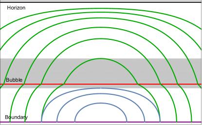
Figure 8: Two spatial geodesics which are anchored at the same interval at the boundary. [Parameters: $\ell_{+}=2$, $M_{+}=0.8$, $\ell_{-}=1$, $M_{-}=0.1$, $Z=1$, $t_{0}=0$, $x_{0}=0$, the bubble shadow is $0.89<z_{0}<1.68$ and the corresponding critical boundary interval is $4.91$].

4 Holographic reconstruction of static BTZ bubbles

A spacetime manifold is a set of points accompanied with a Lorentzian metric. The challenge in establishing a holographic dialogue lies in reconstructing the information that has been projected from the bulk onto the boundary. In order to reconstruct a bulk spacetime, one requires either differential information on the bulk, or causal ordering together with a notion of volume. Here we explore two different methods for reconstructing the bulk, first a differential approach using a prescription for defining points then a definition of distance, and second a causal approach, using the structure of bulk light-cones.

4.1 Bulk reconstruction using entanglement entropy

In Balasubramanian:2013lsa ; Czech:2014ppa , a prescription to reconstruct bulk spacetimes dual to a $1+1$ dimensional CFT was proposed, specifically with spacetime translation invariance. Entanglement entropy of an interval in the boundary CFT is equivalent to the length of the corresponding bulk geodesic joining the end points. Thus broadly speaking, intervals of different length sample different depths in the bulk, however a method for extracting the local spacetime structure is required. The approach of Balasubramanian:2013lsa ; Czech:2014ppa was to first note that a curve $\gamma(\tau)$ in the bulk, where $\tau$ is an arbitrary parameter on the curve, can be described on the boundary via a sequence of intervals, each of which is connected by a bulk geodesic that touches the bulk curve at, and tangent to, a point. This sequence of intervals is expressed as a boundary function $\alpha(x)$, where $x$ is the centre and $x\pm\alpha(x)$ are the endpoints of the interval. The bulk curve $\gamma(\tau)$ thus corresponds to a particular function $\alpha(x)$ on the boundary. The length of $\gamma(\tau)$ has a special interpretation in the bulk; it computes the so called differential entropy Balasubramanian:2013lsa of $\alpha(x)$,

$$E[\alpha]\equiv\frac{1}{2}\int\mathrm{d}x\left.\frac{\mathrm{d}S(\alpha)}{\mathrm{d}\alpha}\right|_{\alpha=\alpha(x)}=\frac{\text{Length}[\gamma]}{4G_{3}}.$$ (33)

Here $S(\alpha)$ denotes the entanglement entropy (or entwinement) corresponding to a boundary interval of length $L=2\alpha$.

Having identified functions on the boundary with curves in the bulk, we then identify a subset of the boundary functions that correspond to bulk points. To do this, simply note that a point is a limit of a sequence of closed curves with length and spanning area tending to zero. To be precise, a point boundary function $\alpha_{p}(x)$ corresponding to a point $p$ in the bulk is a sequence of intervals at the boundary, subtended by the geodesics passing from the point $p$. Therefore, the point boundary functions are a family of boundary functions parametrized by 3 parameters — coordinates of the associated point in the bulk. By definition, the differential entropy of a point boundary function vanishes $E[\alpha_{p}]=0$, which gives a necessary, but not sufficient, condition to determine them.

Point boundary functions are crucial to this bulk-reconstruction scheme, as they provide a boundary interpretation of the bulk manifold. Furthermore, as showed by Czech:2014ppa , given two points $p$ and $q$ in the bulk, geodesic distance between them can be computed using the corresponding point boundary functions $\alpha_{p}(x)$ and $\alpha_{q}(x)$

$$D(p,q)=D[\alpha_{p},\alpha_{q}]\equiv\frac{1}{2}|E[\min(\alpha_{p},\alpha_{q})]|.$$ (34)

The boundary function $\min(\alpha_{p},\alpha_{q})(x)$ is defined quite intuitively as

$$\min(\alpha_{p},\alpha_{q})(x)=\begin{cases}\alpha_{p}(x),&\quad\alpha_{p}(x)<\alpha_{q}(x),\\ \alpha_{q}(x),&\quad\alpha_{p}(x)\geq\alpha_{q}(x).\end{cases}$$ (35)

Consequently, if we are given the family of point boundary functions, and the entanglement (plus entwinement) profile of the boundary, we can reconstruct the bulk spacetime points and their mutual distances, hence recovering the bulk geometry.

4.1.1 Point boundary functions for BTZ black holes

A crucial part of the aforementioned reconstruction scheme is to be able to work out the family of point-boundary functions for a given CFT, without invoking the holographic bulk. As we mentioned above, a necessary condition for a boundary function $\alpha(x)$ to be a point boundary function is that $E[\alpha]=0$, however it is not sufficient. To get some insight into the generic prescription, we start with the family of point boundary functions when we know that the holographic dual is a BTZ black hole geometry.

Consider a point $p=(x_{p},z_{p})$ on a spatial slice of a BTZ black hole with mass $M$ and AdS radius $\ell$. In section 2.2 we established that the family of spatial geodesics can be characterized by their turning point $p_{0}=(x_{0},z_{0})$ in the bulk. Requiring these geodesics to pass the point $p$ determines $|x_{0}-x_{p}|$ leaving a family of geodesics depending on $z_{0}\geq 0$ and $\operatorname{sgn}(x_{0}-x_{p})$. By working out the intersection of these geodesics with the boundary and defining a parameter $\lambda=z_{0}\operatorname{sgn}(x_{0}-x_{p})$, point boundary functions can be expressed parametrically as (see eqs. 13 and 29)

$$\alpha_{p}(\lambda)=\frac{\ell}{\sqrt{M}}\mathcal{S}^{-1}[0,\lambda,M],\qquad x(\lambda)=x_{p}+\operatorname{sgn}(\lambda)\frac{\ell}{\sqrt{M}}\mathcal{S}^{-1}[z_{p},\lambda,M].$$ (36)

On the other hand, the entanglement function for these boundary functions is given by the length of the geodesics given in eq. 27 leading to

$$S(\lambda)=2\ell\log\left(\frac{2|\lambda|/\epsilon}{\sqrt{1-M\lambda^{2}}}\right).$$ (37)

Authors in Czech:2014ppa noted that these point boundary functions obey a curious relation independent of the black hole parameters $\ell$ and $M$

$$\left(1-{\alpha^{\prime}(x)}^{2}\right)\left.\frac{\mathrm{d}^{3}S(\alpha)}{\mathrm{d}\alpha^{3}}\right|_{\alpha=\alpha(x)}+2\alpha^{\prime\prime}(x)\left.\frac{\mathrm{d}^{2}S(\alpha)}{\mathrm{d}\alpha^{2}}\right|_{\alpha=\alpha(x)}=0.$$ (38)

This is a second order ordinary differential equation for $\alpha(x)$, and hence completely determines the two parameter family of point boundary functions. Given that there is no explicit reference to parameters of the bulk in this relation, one might wonder if it holds true in general, and if it could be used as a boundary definition of point boundary functions. One can in fact write down an action

$$I[\alpha]=\int\mathrm{d}x\sqrt{-\left(1-{\alpha^{\prime}(x)}^{2}\right)\left.\frac{\mathrm{d}^{2}S(\alpha)}{\mathrm{d}\alpha^{2}}\right|_{\alpha=\alpha(x)}},$$ (39)

whose extrema lies at the point boundary functions. From the point of view of a bulk curve $\gamma(\tau)$ associated with $\alpha(x)$, the action is merely $\int_{\gamma}d\tau\sqrt{h}K$ where $d\tau\sqrt{h}$ is the line element on $\gamma(\tau)$, while $K$ is the extrinsic curvature. Due to the Gauss-Bonnet theorem in negatively curved spacetimes, this integral extremizes curves enclosing zero area, i.e. points.

These hints lead the authors of Czech:2014ppa to conjecture that perhaps the action eq. 39 is more generic and can be used to isolate point boundary functions in more generic translationally invariant boundary field theories. In the following subsection, we provide a counter example of this naive expectation using our BTZ bubbles. In the absence of a universal bulk independent mechanism to find point boundary functions, this bulk reconstruction mechanism is incomplete.

4.1.2 Point boundary functions for bubbles

We now turn our attention to point boundary functions for BTZ bubbles, and inspect if they agree with the naive differential equation (38). Let us first consider a point $p=(x_{p},z_{p})$ outside the bubble in “$+$” spacetime, i.e. $z_{p}<Z$. Geodesics passing through $p$ are of one of the two types: either they turn outside the bubble staying in “$+$” spacetime all the while, or they penetrate the bubble and turn in “$-$” spacetime. Denoting the turning point by $p_{0}=(x_{0},z_{0})$, we can find the center of the boundary interval (which is merely $x_{0}$ by symmetry) using eqs. 19 and 20, and requiring that the geodesic passes the point $p$

$$x(\lambda)=x_{p}+\operatorname{sgn}(\lambda)\frac{\ell_{+}}{\sqrt{M_{+}}}\bigg{(}\mathcal{S}^{-1}\left[z_{p},\lambda,M_{+}\right]-\Theta(|\lambda|-Z)\mathcal{S}^{-1}\left[Z,\lambda,M_{+}\right]\bigg{)}\\ +\operatorname{sgn}(\lambda)\Theta(|\lambda|-Z)\frac{\ell_{-}}{\sqrt{M_{-}}}\mathcal{S}^{-1}\left[Z,\lambda,M_{-}\right].$$ (40)

As in the bubble-free case, we have defined $\lambda=z_{0}\operatorname{sgn}(x_{0}-x_{p})$. On the other hand, for the point $p$ behind or on the bubble in “$-$” spacetime, i.e. $z_{p}\geq Z$, every geodesic must turn in “$-$” spacetime, hence $z_{0}\geq Z$ as well. In this case, using eqs. 19 and 20 the center of the boundary interval is given as

$$x(\lambda)=x_{p}+\operatorname{sgn}(\lambda)\frac{\ell_{-}}{\sqrt{M_{-}}}\mathcal{S}^{-1}\left[z_{p},\lambda,M_{-}\right].$$ (41)

Now to specify the point boundary functions, we just need the length of the boundary interval subtended by a spatial geodesic in terms of the turning point. We can directly borrow the results from eq. 29 to get

$$\alpha(\lambda)=\frac{\ell_{+}}{\sqrt{M_{+}}}\bigg{(}\mathcal{S}^{-1}[0,\lambda,M_{+}]-\Theta(|\lambda|-Z)\mathcal{S}^{-1}[Z,\lambda,M_{+}]\bigg{)}\\ +\Theta(|\lambda|-Z)\frac{\ell_{-}}{\sqrt{M}_{-}}\mathcal{S}^{-1}[Z,\lambda,M_{-}].$$ (42)

In summary, eq. 42 along with eq. 40 for a point in front of the bubble ($|\lambda|<Z$) and eq. 41 for a point behind the bubble ($|\lambda|\geq Z$) parametrically specify the entire set of point boundary functions for a bubble geometry.

Finally, we compute the entanglement function $S(\lambda)$ by computing the length of the aforementioned geodesics. Using section 3.2 we get

$$S(\lambda) =2\ell_{+}\left[\log\left(\sqrt{\frac{4\lambda^{2}/\epsilon^{2}}{1-M_{+}\lambda^{2}}}\right)-\Theta(|\lambda|-Z)\sinh^{-1}\left(\sqrt{\frac{Z^{-2}-\lambda^{-2}}{\lambda^{-2}-M_{+}}}\right)\right]$$

$$\qquad+2\Theta(|\lambda|-Z)\ell_{-}\sinh^{-1}\left(\sqrt{\frac{Z^{-2}-\lambda^{-2}}{\lambda^{-2}-M_{-}}}\right).$$ (43)

We wish to see whether the point boundary functions satisfy the bulk independent differential equations (38). To do so, it is helpful to decompose eq. 38 in terms of an intermediate parameter $\lambda$ to give

$$3\alpha^{\prime\prime}(\chi){\alpha^{\prime}(\chi)}^{2}+\frac{2}{\chi missing}{\alpha^{\prime}(\chi)}^{3}\overset{?}{=}{x^{\prime}(\chi)}^{2}\left(\frac{2}{\chi missing}\alpha^{\prime}(\chi)+\alpha^{\prime\prime}(\chi)\right)+2\frac{x^{\prime\prime}(\chi)}{x^{\prime}(\chi)}{\alpha^{\prime}(\chi)}^{3},$$ (44)

where all the derivatives are taken with respect to the parameter $\chi$. We have used the fact that $S^{\prime}(\chi)=\frac{2}{|\chi|}\alpha^{\prime}(\chi)$ to simplify the equation, which can be checked to hold explicitly on the point boundary functions associated with bubble or BTZ geometries. Plugging the point boundary functions in eqs. 42, 40 and 41 into this differential equation, we can check that it indeed is not satisfied as we claimed.

Using this counter-example, we see that point boundary functions for generic holographic CFT’s cannot, in fact, be generated using the action in eq. 39. Another plausible mechanism to figure out point boundary functions was suggested in the appendix of Czech:2015qta , which among other things, assumes the bulk to not have any pair of conjugate points (points connected by more than one geodesics). As we discussed in section 2.2, this assumption severely breaks down in the presence of bubbles. Bubbles, as we constructed them, exemplify the simplest form of extended matter in the bulk which confirms with the symmetries of the boundary, hence we expect that the assumptions in Czech:2015qta will continue to be invalid in bulk spacetimes with arbitrary matter distribution. Other methods include using geodesics in boundary Kinematic space as an alternative definition of point boundary functions, but as we show in appendix A, they do not work with bubbles either. We conclude that a more generic bulk-independent mechanism to define point boundary functions in the field theory is required for this bulk reconstruction prescription to be complete.

4.2 Light-cone cuts

In a recent paper Engelhardt:2016wgb (see also Engelhardt:2016crc ; Engelhardt:2016vdk ), Engelhardt and Horowitz proposed a new mechanism to reconstruct the metric of a spacetime, up to a conformal factor, using its holographic dual. Unlike hole-ography however, which relies on the entanglement structure of the boundary field theory, this prescription makes use of the divergence structure of ($d+2$)-point correlation functions in the field theory to reconstruct the $(d+1)$-dimensional bulk metric. The proposal involves a novel field theory observable called “light-cone cuts” defined as the hypersurfaces that are null separated from a point in the dual bulk. These cuts can be used to reconstruct the metric, up to a conformal factor, for a part of the bulk that is in causal contact with the boundary. From a purely field theoretic perspective, light-cone cuts can be obtained using the divergence structure of $(d+2)$-point correlation functions.

In the following, we give a quick review of the reconstruction procedure of Engelhardt:2016wgb , presented in a slightly different language than the original material. To a given point $p$ in the causally visible bulk (from the boundary), we can associate a unique cut $C_{p}$ at the boundary defined as the intersection of the boundary with the light-cone of $p$. Engelhardt and Horowitz further showed that distinct bulk points cannot lead to the same cut, establishing a bijection between the set of cuts, which we refer to as the “cut-space”, and points in the causally visible bulk. From the bulk point of view, it is clear that the cut-space should be a $(d+1)$-parameter family of hypersurfaces in the $d$-dimensional boundary. Hence a cut in the family can be represented as $C_{\lambda}$ where $\lambda=(\lambda^{0},\ldots,\lambda^{d})$ is an arbitrary set of parameters. Given the bijection, $\lambda$ can also serve as a coordinate system in the causally visible bulk. On a given cut $C_{\lambda}$, we will sometimes choose a parametrization $\sigma=(\sigma^{1},\ldots,\sigma^{d-1})$ and denote a point on the cut as $C^{i}_{\lambda}(\sigma)$ where the index $i$ refers to the boundary coordinates.

One can make a curious observation in the setup defined above. Consider a point with coordinates $\lambda_{0}$ in the causally visible bulk and the corresponding cut $C_{\lambda_{0}}$ at the boundary; if another point $\lambda$ in the bulk is null separated from $\lambda_{0}$, then the associated cut $C_{\lambda}$ intersects $C_{\lambda_{0}}$ tangentially at the boundary. That the two cuts intersect follows trivially from the fact that the light ray joining $\lambda$ to $\lambda_{0}$ hits the boundary at some point $\sigma_{0}$ which lies on both the cuts. Furthermore, let $\lambda$ be in the future of $\lambda_{0}$, then the entire causal future of $\lambda$ is visible to $\lambda_{0}$ while $\lambda$ can see the entire past of $\lambda_{0}$, and vice-versa if $\lambda$ is in the past of $\lambda_{0}$. If the cuts were to cross, and not intersect tangentially, at least one of these conditions will be violated.

The more interesting part of this observation is the converse, which is the backbone of this reconstruction mechanism. Let $C_{\lambda_{0}}$ be a cut at the boundary, then all the cuts $C_{\lambda}$ that intersect $C_{\lambda_{0}}$ tangentially at some point $\sigma_{0}$, trace out a curve in the $\lambda$-space (i.e. cut-space) which corresponds to a light ray in the bulk passing through the point $\lambda_{0}$ and hitting the boundary at the point $\sigma_{0}$. It is obviously a curve, as opposed to a higher dimensional surface, because $\lambda$ is a set of $(d+1)$ parameters and the condition of tangential intersection imposes $d$ constraints on it, leaving one free parameter defining the curve. Since we know that the cuts corresponding to the points on a light ray joining $\lambda_{0}$ with $\sigma_{0}$ must be tangential to $C_{\lambda_{0}}$ at $\sigma_{0}$, this light ray must be the unknown curve in question.

The philosophy of reconstruction this point forth is rather straightforward: we assume that we are provided with a family of light-cone cuts $C_{\lambda}$ at the boundary with some arbitrary parametrization $\lambda$. We will come back to the question of determining this family using the field theory data in a while. Given a particular cut $C_{\lambda_{0}}$ in this family and a point parametrized by $\sigma_{0}$ on $C_{\lambda_{0}}$, we will look for a curve $\gamma_{(\lambda_{0},\sigma_{0})}$ in the $\lambda$-space which corresponds to cuts tangent to $C_{\lambda_{0}}$ at the point $\sigma_{0}$. $\gamma_{(\lambda_{0},\sigma_{0})}$ can be defined via the tangential intersection constraints

$$C_{\lambda}^{i}(\sigma)=C_{\lambda_{0}}^{i}(\sigma_{0}),\qquad\frac{\mathrm{d}missing}{\mathrm{d}\sigma missing}C^{i}_{\lambda}(\sigma)\propto\left.\frac{\mathrm{d}missing}{\mathrm{d}\sigma missing}C^{i}_{\lambda_{0}}(\sigma)\right|_{\sigma=\sigma_{0}}\qquad\text{for some}\leavevmode\nobreak\ \sigma.$$ (45)

Obviously the point $\lambda_{0}$ lies on $\gamma_{(\lambda_{0},\sigma_{0})}$. We denote the tangent vector to $\gamma_{(\lambda_{0},\sigma_{0})}$ at the point $\lambda_{0}$ as $n^{a}_{(\lambda_{0},\sigma_{0})}$, where the index $a$ runs from $0$ to $d$. We know that from the point of view of the bulk, $n^{a}_{(\lambda_{0},\sigma_{0})}$ must be a null vector. So we define a metric $g_{ab}(\lambda)$ on the $\lambda$-space such that it gives zero norm to $n^{a}_{(\lambda_{0},\sigma_{0})}$

$$g_{ab}(\lambda_{0})n^{a}_{(\lambda_{0},\sigma_{0})}n^{b}_{(\lambda_{0},\sigma_{0})}=0.$$ (46)

We can repeat this procedure for as many values of $\sigma_{0}$ as we like, making the system overdetermined for $g_{ab}(\lambda_{0})$. If the boundary field theory is indeed holographic, there must exist at least one value of $g_{ab}(\lambda_{0})$ which satisfies eq. 46 for all values of $\sigma_{0}$. Note that $g_{ab}(\lambda_{0})$ has $\frac{1}{2}(d+1)(d+2)$ independent components, but a conformal factor can never be determined through eq. 46. Nevertheless, we can choose $\frac{1}{2}(d+1)(d+2)-1=\frac{1}{2}d(d+3)$ generic values of $\sigma_{0}$ and determine the metric $g_{ab}(\lambda_{0})$ at the point $\lambda_{0}$ up to a conformal factor. We can then go ahead and repeat this procedure for all values of $\lambda_{0}$ to determine the conformal metric in the entire causally visible bulk.

Now for the reconstruction procedure to be complete, up to a conformal factor, we just need a field theoretic definition of light-cone cuts. Maldacena:2015iua argued that an $n$-point Lorentzian correlator in a holographic field theory can diverge if all its points are null separated from a bulk point, given that we can associate null momenta to each of the points while conserving energy-momentum at the bulk point. Let us consider a set of $d+1$ points $\{x_{1},\ldots,x_{d+1}\}$ in a $d$-dimensional holographic field theory, so that there is a unique point $p$ in the bulk which is null separated from all $x_{i}$. Let us also take two more points $z_{1}$ and $z_{2}$ at the boundary, so that the following correlator diverges,

$$\Big{<}\mathcal{O}(z_{1})\mathcal{O}(z_{2})\mathcal{O}(x_{1})\dots\mathcal{O}(x_{d+1})\Big{>}\rightarrow\infty.$$ (47)

For this to happen, the point $z_{1}$ can be anywhere on the light-cone cut corresponding to the bulk point $p$, while $z_{2}$ should be another point on the cut so that the energy-momentum at $p$ is conserved. Now we can find light-cone cuts by fixing some points $\{x_{i}\}$ at the boundary — which fixes the bulk point $p$ — and tracing the points $z_{1}$, $z_{2}$ at the boundary, so that the $(d+3)$-point correlator in eq. 47 remains divergent. Once we have the cuts, we can go ahead and reconstruct the bulk metric, up to a conformal factor.

Above, we gave an extremely compact review of bulk reconstruction via light-cone cuts. Naturally, we had to gloss over a lot of tiny yet important details, which can be found in Engelhardt:2016wgb . In the following we will now try to explicitly reconstruct our static BTZ bubble using this method. This might help better understand the prescription by applying to a non-trivial geometry in presence of matter.

4.2.1 Light-cone cuts for BTZ black hole

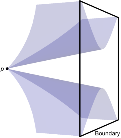
(a)

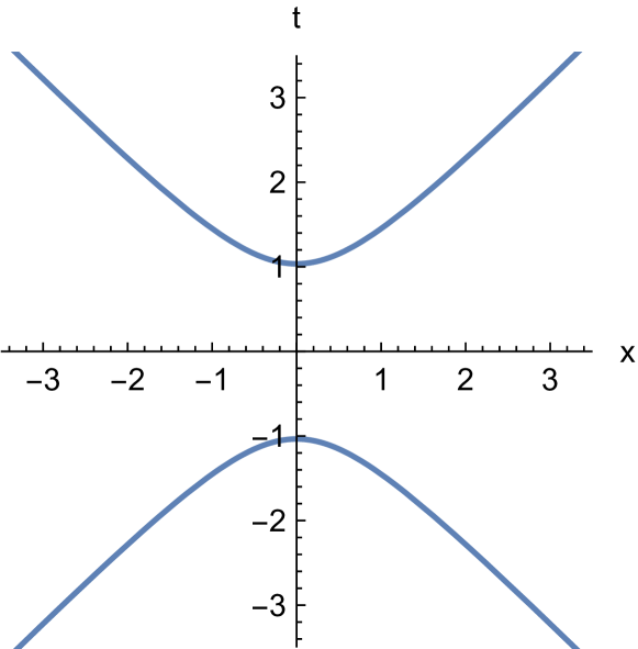
(b)

Figure 9: (a) Part of the light-cone originating at a point $p$ in the bulk. (b) A generic light-cone cut at the boundary. (Parameters: $\ell=1$, $M=0.1$ and $p=(0,0,1)$).

For simplicity, let us start an ordinary BTZ black hole whose metric has been given in eq. 1. A generic null geodesic in this geometry, which escapes to the boundary, is given in eq. 21. To find the light-cone cuts, we need to trace the trajectory of the boundary point $(t_{0},x_{0})$ in eq. 21 for all the null geodesics that pass through some point $(t_{p},x_{p},z_{p})$ in the bulk. We find

$$C^{t}_{\lambda}(\sigma)=\lambda^{0}\mp\frac{1}{\sqrt{\mu}}\mathcal{T}^{-1}_{t}[\lambda^{2},\sigma,\mu],\qquad C^{x}_{\lambda}(\sigma)=\lambda^{1}\mp\frac{1}{\sqrt{\mu}}\mathcal{T}^{-1}_{x}[\lambda^{2},\sigma,\mu],$$ (48)

where $\mu=M/\ell^{2}$ is the only parameter on which the family of light-cone cuts depends, and not on the parameters $M$ and $\ell$ independently. This can be traced back to the fact that under a scaling $M\rightarrow M\Omega^{2}$, $\ell\rightarrow\ell\Omega$, $z\rightarrow z/\Omega$, the metric changes by a conformal factor $\Omega^{2}$, leaving light-cones and hence the light-cone cuts invariant. The set $\lambda=(\lambda^{0}=t_{p},\lambda^{1}=x_{p},\lambda^{2}=\ell z_{p})$ can be understood as coordinates in the cut-space, while the momentum $\sigma=p$ is a parameter on the cut. Eliminating $\sigma$, we can write down a constraining equation for the light-cone cuts

$$\tanh^{2}\left(\sqrt{\mu}(C^{t}-\lambda^{0})\right)-\left(1-\mu{(\lambda^{2})}^{2}\right)\tanh^{2}\left(\sqrt{\mu}(C^{x}-\lambda^{1})\right)=\mu{(\lambda^{2})}^{2}.$$ (49)

See figure 9 for a graphical illustration. Interestingly in the AdS limit, i.e. when the black hole mass $M\rightarrow 0$, light-cone cuts become hyperbolas,

$${(C^{t}-\lambda^{0})}^{2}-{(C^{x}-\lambda^{1})}^{2}={(\lambda^{2})}^{2},$$ (50)

which are independent of the AdS radius $\ell$. This is expected, because in pure AdS we can always transform away $\ell$ to a conformal factor.

Reconstruction:

We will now forget about the bulk, and will assume that these light-cone cuts can be obtained directly by a field theory computation. Such a computation, in general, might lead to an arbitrarily different parametrization of the cuts. The metric thus obtained via the reconstruction prescription, will be related to the one given in eq. 1 by merely a coordinate transformation and an arbitrary conformal factor.

Plugging the light-cone cuts in eq. 48 into eq. 45, a straightforward computation will lead to the null generators

$$n^{a}_{(\lambda,\sigma)}\propto\left(\pm\frac{1}{1-\mu{(\lambda^{2})}^{2}}\leavevmode\nobreak\ ,\leavevmode\nobreak\ \pm\sigma\leavevmode\nobreak\ ,\leavevmode\nobreak\ \sqrt{1-\sigma^{2}(1-\mu{(\lambda^{2})}^{2})}\right).$$ (51)

Defining a metric $g_{ab}\mathrm{d}\lambda^{a}\mathrm{d}\lambda^{b}$, eq. 46 then takes the form

$$\frac{1}{1-\mu{(\lambda^{2})}^{2}}\left(\frac{g_{00}}{1-\mu{(\lambda^{2})}^{2}}+g_{22}(1-\mu{(\lambda^{2})}^{2})\right)+\sigma^{2}\left(g_{11}-g_{22}(1-\mu{(\lambda^{2})}^{2})\right)\\ +\frac{2\sigma g_{01}}{1-\mu{(\lambda^{2})}^{2}}\pm 2\left(\sigma g_{12}+\frac{g_{02}}{1-\mu{(\lambda^{2})}^{2}}\right)\sqrt{1-\sigma^{2}(1-\mu{(\lambda^{2})}^{2})}=0.$$ (52)

Since this equation must be imposed for all values of $\sigma$, we can perform a Taylor expansion around $\sigma=0$ and set all the coefficients to zero. For example, the coefficients of $\sigma^{3}$ and $\sigma^{4}$ only get contributions from the last term and set $g_{12}=g_{02}=0$. The coefficient of $\sigma$ then sets $g_{01}=0$, while the coefficients of $\sigma^{2}$ and $1$ determine the metric up to an arbitrary overall factor

$$\mathrm{d}s^{2}=\Omega^{2}(\lambda)\left[-\left(1-\mu{(\lambda^{2})}^{2}\right){(\mathrm{d}\lambda^{0})}^{2}+{(\mathrm{d}\lambda^{1})}^{2}+\frac{1}{1-\mu{(\lambda^{2})}^{2}}{(\mathrm{d}\lambda^{2})}^{2}\right].$$ (53)

Choosing the conformal factor $\Omega(\lambda)=\ell/\lambda^{2}$ and picking a basis $\{\lambda^{0}=t,\lambda^{1}=x,\lambda^{2}=\ell z\}$, we can recover the BTZ metric in eq. 1 with mass $M=\mu\ell^{2}$.

4.2.2 Light-cone cuts for bubbles

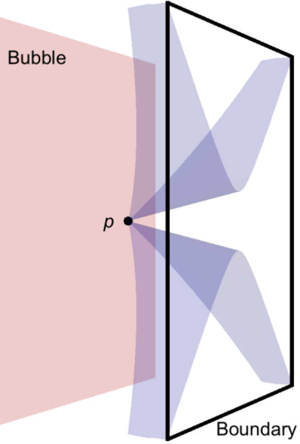
(a)

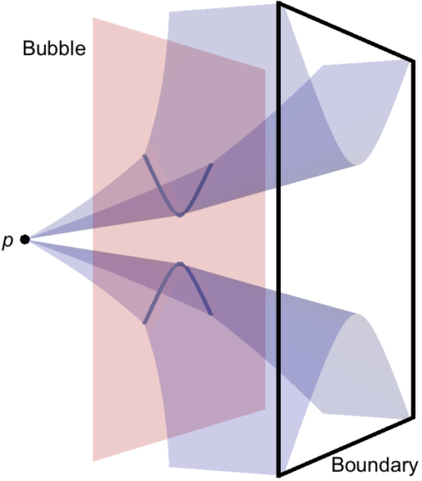
(b)

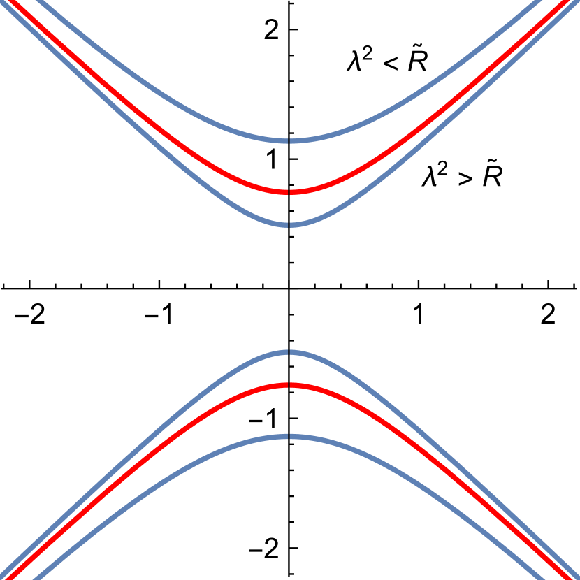
(c)

Figure 10: Part of the light-cone originating at a point $p$ in the bulk (a) in front of the bubble and (b) behind the bubble. (c) A generic set of light-cone cuts at the boundary; the one in red corresponds to a $\lambda^{2}=R$ (i.e. when the corresponding bulk point is on the bubble). (Parameters: $\ell_{+}=1$, $M_{+}=0.1$, $\ell_{-}=0.5$, $M_{-}=0.05$, $R=0.75$ and $p=(0,0,0.5),(0,0,1.5)$).

We now move on to the case of static BTZ bubbles. Similar to our calculation in the previous section, we can use null geodesics for bubbles given in eqs. 23 and 22 to work out the light cone cuts. We trace the trajectory of the point $(t_{0},x_{0})$ in eqs. 23 and 22 while requiring the null geodesics to pass a fixed point $(t_{p},x_{p},z_{p})$ in the “$+$” part of the bulk or equivalently $(\gamma t_{p},x_{p},z_{p})$ in the “$-$” part. We find

$$C^{t_{+}}_{\lambda}(\sigma) =\lambda^{0}\mp\frac{1}{\sqrt{\mu_{+}}}\bigg{[}\mathcal{T}_{t}^{-1}[\lambda^{2},\sigma,\mu_{+}]-\Theta(\lambda^{2}-\zeta_{+})\Big{(}\mathcal{T}_{t}^{-1}[\lambda^{2},\sigma,\mu_{+}]-\mathcal{T}_{t}^{-1}[\zeta_{+},\sigma,\mu_{+}]\Big{)}\bigg{]}$$

$$\qquad\mp\Theta(\lambda^{2}-\zeta_{+})\frac{1}{\gamma missing}\frac{1}{\sqrt{\mu_{-}}}\Big{(}\mathcal{T}_{t}^{-1}[\zeta\lambda^{2},\gamma\sigma,\mu_{-}]-\mathcal{T}_{t}^{-1}[\zeta_{-},\gamma\sigma,\mu_{-}]\Big{)},$$

$$C^{x}_{\lambda}(\sigma) =\lambda^{1}\mp\frac{1}{\sqrt{\mu_{+}}}\bigg{[}\mathcal{T}_{x}^{-1}[\lambda^{2},\sigma,\mu_{+}]-\Theta(\lambda^{2}-\zeta_{+})\left(\mathcal{T}_{x}^{-1}[\lambda^{2},\sigma,\mu_{+}]-\mathcal{T}_{x}^{-1}[\zeta_{+},\sigma,\mu_{+}]\right)\bigg{]}$$

$$\qquad\mp\Theta(\lambda^{2}-\zeta_{+})\frac{1}{\sqrt{\mu_{-}}}\left(\mathcal{T}_{x}^{-1}[\zeta\lambda^{2},\gamma\sigma,\mu_{-}]-\mathcal{T}_{x}^{-1}[\zeta_{-},\gamma\sigma,\mu_{-}]\right).$$ (54)

Here again, we have defined a set of coordinates $\lambda=(\lambda^{0}=t_{p},\lambda^{1}=x_{p},\lambda^{2}=\ell_{+}z_{p})$ on the cut-space, and $\sigma=p_{0}$ is a parameter on the cut. We have also condensed the parametric dependence of the cuts into four dimensionless combinations

$$\mu_{\pm}=\frac{M_{\pm}}{\ell_{\pm}^{2}},\qquad\zeta_{\pm}=Z\ell_{\pm},$$ (55)

and defined $\zeta=\zeta_{-}/\zeta_{+}=\ell_{-}/\ell_{+}$. In terms of these, $\gamma=\sqrt{\frac{1-\mu_{+}\zeta_{+}^{2}}{1-\mu_{-}\zeta_{-}^{2}}}$. The information about one independent parameter out of $M_{\pm}$, $\ell_{\pm}$ and $Z$ is lost. See figure 10. Interestingly, when the bubble is on an AdS-AdS interface, i.e. $M_{\pm}\rightarrow 0$, the light-cone cuts reduce to

$$\begin{split}\lim_{M_{\pm}\rightarrow 0}C^{t_{+}}_{\lambda}(\sigma)&=\lambda^{0}\mp\frac{1}{\sqrt{1-\sigma^{2}}}\left[\lambda^{2}+\Theta(\lambda^{2}-\zeta_{+})\left(\zeta\lambda^{2}-\lambda^{2}-\zeta_{-}+\zeta_{+}\right)\right],\\ \lim_{M_{\pm}\rightarrow 0}C^{x}_{\lambda}(\sigma)&=\lambda^{1}\mp\frac{\sigma missing}{\sqrt{1-\sigma^{2}}}\left[\lambda^{2}+\Theta(\lambda^{2}-\zeta_{+})\left(\zeta\lambda^{2}-\lambda^{2}-\zeta_{-}+\zeta_{+}\right)\right].\end{split}$$ (56)

Note that we can remove all the parametric dependence by performing a coordinate transformation in the cut-space: $\lambda^{2}\to\lambda^{\prime 2}=\lambda^{2}+\Theta(\lambda^{2}-\zeta_{+})\left(\zeta\lambda^{2}-\lambda^{2}-\zeta_{-}+\zeta_{+}\right)$, after which they merely reduce to their bubble-free hyperbolic form given in eq. 50. Hence we can infer that the cut-space of an AdS-AdS bubble is same as that of a bubble-free AdS.

Reconstruction:

Having obtained the light-cone cuts section 4.2.2, we can now forget about the bulk and try to reconstruct it using the boundary data. Similar to the ordinary BTZ case, the normal vector $n^{a}_{(\lambda,\sigma)}$ can be obtained by solving eq. 45. We find that for “$+$” spacetime we have

$$n^{a}_{(\lambda,\sigma)}\propto\left(\leavevmode\nobreak\ \pm\frac{1}{1-\mu_{+}{(\lambda^{2})}^{2}}\leavevmode\nobreak\ ,\leavevmode\nobreak\ \pm\sigma\leavevmode\nobreak\ ,\leavevmode\nobreak\ \sqrt{1-\sigma^{2}\left(1-\mu_{+}{(\lambda^{2})}^{2}\right)}\leavevmode\nobreak\ \right).$$ (57)

while for “$-$” spacetime

$$n^{a}_{(\lambda,\sigma)}\propto\left(\leavevmode\nobreak\ \pm\frac{1/\gamma missing}{1-\mu_{-}{(\zeta\lambda^{2})}^{2}}\leavevmode\nobreak\ ,\leavevmode\nobreak\ \pm\gamma\sigma\leavevmode\nobreak\ ,\leavevmode\nobreak\ \frac{1}{\zeta}\sqrt{1-\gamma^{2}\sigma^{2}\left(1-\mu_{-}{(\zeta\lambda^{2})}^{2}\right)}\right).$$ (58)

Putting this back in eq. 46 we get the constraints: in the “$+$” spacetime

$$\frac{1}{1-\mu_{+}{(\lambda^{2})}^{2}}\left(\frac{g_{00}}{1-\mu_{+}{(\lambda^{2})}^{2}}+g_{22}\left(1-\mu_{+}{(\lambda^{2})}^{2}\right)\right)+\sigma^{2}\Big{(}g_{11}-g_{22}\left(1-\mu_{+}{(\lambda^{2})}^{2}\right)\Big{)}\\ \pm 2\left(\frac{g_{02}}{1-\mu_{+}{(\lambda^{2})}^{2}}+\sigma g_{12}\right)\sqrt{1-\sigma^{2}\left(1-\mu_{+}{(\lambda^{2})}^{2}\right)}+\frac{2\sigma g_{10}}{1-\mu_{+}{(\lambda^{2})}^{2}}=0,$$ (59)

and in the “$-$” spacetime

$$\frac{1}{1-\mu_{-}{(\zeta\lambda^{2})}^{2}}\left(\frac{g_{00}/\gamma^{2}}{1-\mu_{-}{(\zeta\lambda^{2})}^{2}}+g_{22}\frac{1-\mu_{-}{(\zeta\lambda^{2})}^{2}}{\zeta^{2}}\right)+\gamma^{2}\sigma^{2}\left(g_{11}-g_{22}\frac{1-\mu_{-}{(\zeta\lambda^{2})}^{2}}{\zeta^{2}}\right)\\ \pm\frac{2}{\zeta missing}\left(\frac{g_{02}/\gamma missing}{1-\mu_{-}{(\zeta\lambda^{2})}^{2}}+\gamma\sigma g_{12}\right)\sqrt{1-\gamma^{2}\sigma^{2}\left(1-\mu_{-}{(\zeta\lambda^{2})}^{2}\right)}+\frac{2\sigma g_{10}}{1-\mu_{-}{(\zeta\lambda^{2})}^{2}}=0.$$ (60)

Again performing a Taylor expansion in $\sigma$ we can find that the metric must be diagonal. In fact up to a conformal factor $\Omega^{2}(\lambda)$ we get

$$ds^{2}=\begin{cases}\displaystyle\Omega^{2}(\lambda)\left[-\left(1-\mu_{+}{(\lambda^{2})}^{2}\right){(d\lambda^{0})}^{2}+{(d\lambda^{1})}^{2}+\frac{1}{1-\mu_{+}{(\lambda^{2})}^{2}}{(d\lambda^{2})}^{2}\right],&\lambda^{2}\geq\zeta_{+}\\ \displaystyle\Omega^{2}(\lambda)\left[-\left(1-\mu_{-}{(\lambda^{2})}^{2}\right){(\gamma d\lambda^{0})}^{2}+{(d\lambda^{1})}^{2}+\frac{\zeta^{2}}{1-\mu_{-}{(\lambda^{2})}^{2}}{(d\lambda^{2})}^{2}\right],&\lambda^{2}<\zeta_{+}.\\ \end{cases}$$ (61)

Choosing the coordinates

$$\lambda^{0}=t_{+}=t_{-}/\gamma,\qquad\lambda^{1}=x,\qquad\lambda^{2}=\ell_{+}z,$$ (62)

and a conformal factor $\Omega(\lambda)=\ell_{+}/\lambda^{2}=1/z$, we can recover the metric in eq. 2 with AdS radii $\ell_{+}$ and $\ell_{-}=\zeta\ell_{+}$, masses $M_{\pm}=\mu_{\pm}\ell_{\pm}^{2}$ and the bubble radius $Z=\zeta_{+}/\ell_{+}=\zeta_{-}/\ell_{-}$.

5 Discussion

In this paper we considered the question of holographic reconstruction of spacetimes containing non-trivial matter. We believe that this is an important consistency check for any bulk reconstruction prescription, which aims to build non-trivial holographic spacetimes using purely boundary observables. Realising that most of the previous work on geometric bulk reconstruction has concerned itself with spacetimes which are quotients of AdS, we chose to work with thin BTZ bubble walls as an example of non-trivial matter content in the bulk. Such a choice of the matter presence has several unique features. On the one hand, it has almost the same amount of symmetries as pure AdS or BTZ black hole, whereas the presence of matter is non-local and the geometry is no longer merely a quotient of AdS. To retain some analytic control over the problem, we have further restricted ourselves to static thin bubble wall solutions. Some readers might argue against such a matter presence as we are explicitly giving away smoothness of the spacetime manifold. However, thin wall bubbles are a well known approximation to the more realistic thick wall solutions, for which the manifold is smooth everywhere. One can easily imagine a sequence of limiting and still smooth thick wall solutions approximating a thin bubble wall. We therefore expect the qualitative features discussed in this paper to be valid for thick bubble walls which are sufficiently thin compared to relevant length scales in the problem. We intend to discuss this issue in detail in a follow-up work PSIStudentsPaper .

An additional advantage of working with bubble spacetimes is that they can provide a toy model for understanding the process of matter collapse and black hole formation in the bulk. From the boundary perspective, this process is understood as thermalisation of a field theory state towards its thermal equilibrium Danielsson:1999fa ; Balasubramanian:2011ur . On the one hand, looking at these non-trivial dynamical processes from the perspective of holographic bulk reconstruction is expected to bring some new and important insights in the long-standing puzzles in (quantum) black hole physics Almheiri:2012rt . On the other hand, they should also guide our efforts towards writing with a universally applicable bulk reconstruction scheme. In any case, it would be interesting to extend the analysis done in this paper to include dynamical thin bubble walls and explore if we find any qualitative differences in the results. Having sacrificed the time translation invariance of our setup, it is likely that explicit results will require numerical techniques. We plan to return to this question in the near future.

We considered two recent schemes of geometric bulk reconstruction. Using the hole-ography method, we are able to reconstruct the metric on a spatial slice of the bulk using the entanglement structure of the boundary, provided we are given a bulk-independent mechanism to work out point boundary functions for a given field theory. Unfortunately, as we discussed in the bulk of this paper, the current mechanism in place to work out these functions using a variational principle seems to break down when applied to bubble geometries. There have also been some suggestions (see e.g. Czech:2016xec ) to use boundary Kinematic spaces to work out the point boundary functions. However, we show in appendix A that this also does not work with bubble geometries. In absence of such a mechanism, the hole-ographic prescription by itself is incomplete, which adds to the limitations of hole-ography previously pointed out in Engelhardt:2015dta .

The light-cone cuts method of Engelhardt:2016wgb , on the other hand, seems to work quite well for bubble spacetimes, considering the manifold we are working with is not smooth due to the presence of a thin wall. It should be noted, as the authors pointed out themselves, that this bulk reconstruction prescription only returns the metric up to a conformal factor. This essentially means that the information about the volume measure is not recoverable in this scheme. In particular, this implies that the light-cone cuts method is ignorant of a thin bubble wall bubble between two empty AdS spacetimes, which is conformally related to an empty AdS. We know that from the boundary field theory perspective, the presence of a dynamical thin shell in an empty AdS spacetime corresponds to an RG flow in the boundary field theory, whereas an empty AdS spacetime corresponds to the vacuum state. Therefore, a lot of such interesting physics is lost in the light-cone cut prescription, unless we can complement it with an independent prescription to compute the volume measure. As a future direction, it would be interesting to explore if the two methods of bulk reconstruction considered here can be made to complement each other, so as to mutually overcome their shortcomings.

Another important direction in the bulk reconstruction program is the ongoing research on tensor networks Almheiri:2014lwa ; Pastawski:2015qua ; Czech:2015kbp . These methods, again, have been quite successful in describing the emergence of locally AdS geometries from boundary field theory data. The natural next step therefore, is to extend this discussion to the cases where non-trivial matter is present in the bulk. A viable toy model to explore this direction is provided by the thin bubble walls discussed in this paper, whose analysis has already been initiated in Czech:2016nxc . Another bulk restriction prescription that we have not considered in this work is using the quantum error correcting structure of AdS/CFT, proposed recently by Sanches:2017xhn . Like the light-cone prescription, it promises to be able to reconstruct the bubble spacetime up to a conformal factor.

During our holographic analysis of thin bubble walls in section 3, we observed the existence of the so called “bubble shadows”: a region around a bubble wall in the bulk spacetime which is only partially probed by minimal geodesics. These appear to be a generalisation of entanglement shadows found around BTZ black holes and conical defects, which are spacetime regions where no minimal geodesics can enter. These preliminary results seem to suggest that such shadows in boundary entanglement structure might be a generic feature of the presence of matter in the bulk. However, more analysis is required before these suggestions can be turned into concrete claims.

Acknowledgements

We would like to thank Mike Appels, Leo Cuspinera, Aurora Ireland and Simon Ross for helpful discussions. The work of PB was supported by the “Quantum Universe” I-CORE program of the Israel Planning and Budgeting Committee. RG is supported in part by STFC Consolidated Grant ST/P000371/1. AJ is supported by Durham Doctoral Scholarship from Durham University. AJ would also like to acknowledge the hospitality provided by Perimeter Institute for Theoretical Physics, Canada where part of this project was done. Research at Perimeter Institute is supported by the Government of Canada through the Department of Innovation, Science and Economic Development Canada and by the Province of Ontario through the Ministry of Research, Innovation and Science.

Appendix A Kinematic space for BTZ bubbles

In this appendix we discuss the kinematic spaces associated with the bubble spacetimes discussed in this paper. For a detailed discussion of Kinematic spaces and their relevance in bulk reconstruction, see Czech:2015qta ; Bhowmick:2017egz ; Czech:2016xec and references therein. A kinematic space, from the boundary field theory perspective, is defined as the space of pair of boundary points. In pure AdS, it can equivalently be defined from the bulk perspective as the space of bulk geodesics anchored at those boundary points. In more complicated spacetimes however, this equivalence runs into some trouble because of the existence of multiple geodesics corresponding to same boundary intervals. For example, AdS spacetime with a conical defect admits multiple geodesics anchored at the same boundary points, labelled by their winding number around the defect. The kinematic space for this geometry was studied in Cresswell:2017mbk . A similar story holds true for cyclically identified BTZ black holes as well, wherein the geodesics wind around the horizon instead of the defect.

As we have explored in this paper, BTZ black holes with bubble walls admit additional geodesics for a subset of boundary intervals, which in a sense are more non-trivial than the ones wrapping around the horizon. To isolate this effect, we specialised to planar BTZ black holes, so that we can concentrate on only the multiple geodesics arising due to the bubble. In this section we would like to explore Kinematic spaces for these bubbles. Let us start with a generic discussion of $(2+1)$-dimensional bulk spacetimes, whose constant time slices look like

$$\mathrm{d}s^{2}=\frac{1}{z^{2}}\Big{(}\mathrm{d}x^{2}+f^{2}(z)\mathrm{d}z^{2}\Big{)},$$ (63)

where $f(z)=f(-z)$. In the case of BTZ bubbles discussed in the bulk of this paper (see metric (2)), $f(z)$ takes a step function profile

$$f^{2}(z)=\frac{\ell^{2}_{+}}{1-M_{+}z^{2}}\Theta(Z-z)+\frac{\ell^{2}_{-}}{1-M_{-}z^{2}}\Theta(z-Z).$$ (64)

Spatial geodesics corresponding to metric (63) are given by a two parameter family

$$x(\zeta)=x_{0}+\operatorname{sgn}(\zeta)\operatorname{sgn}(z_{0})\int_{|z_{0}|-|\zeta|}^{|z_{0}|}\mathrm{d}\lambda\frac{\lambda f(\lambda)}{\sqrt{z_{0}^{2}-\lambda^{2}}},\qquad z(\zeta)=|z_{0}|-|\zeta|.$$ (65)

where $x_{0},z_{0}\in\mathbb{R}$. Note that the way we have parametrised this family of geodesics, it is left invariant by $z_{0}\to-z_{0}$ provided we take the parameter on the geodesic $\zeta\to-\zeta$. Therefore every geodesic is counted twice. In this sense, eq. 65 actually parametrise the set of “oriented spatial geodesics”, where the orientation is defined by $\operatorname{sgn}\left(x^{\prime}(\zeta)\right)=\operatorname{sgn}(z_{0})$. This set is generally known as the “Kinematic space”. The pair of parameters $(x_{0},z_{0})$ serve as a basis on the Kinematic space. Locally, we can also use as basis the $x$-coordinates $(u,v)$ of the points at which the geodesic hits the boundary $z\to 0$, i.e. $\zeta=\pm|z_{0}|$. They are given in terms of $(x_{0},z_{0})$ as

$$u =x(-|z_{0}|)=x_{0}-\operatorname{sgn}(z_{0})\int_{0}^{|z_{0}|}\mathrm{d}\lambda\frac{\lambda f(\lambda)}{\sqrt{z_{0}^{2}-\lambda^{2}}},$$

$$v =x(|z_{0}|)=x_{0}+\operatorname{sgn}(z_{0})\int_{0}^{|z_{0}|}\mathrm{d}\lambda\frac{\lambda f(\lambda)}{\sqrt{z_{0}^{2}-\lambda^{2}}}.$$ (67)

Alternatively, we could also use the local basis $(\alpha,x_{0})$ where

$$\alpha(z_{0})=\frac{v-u}{2}=\operatorname{sgn}(z_{0})\int_{0}^{|z_{0}|}\mathrm{d}\lambda\frac{\lambda f(\lambda)}{\sqrt{z_{0}^{2}-\lambda^{2}}},$$ (68)

is half the signed length of the interval spanned by the geodesic. Note however, that when there are multiple spatial geodesics corresponding to the same boundary interval, such bases are not globally well defined. One can define a measure on the Kinematic space locally via the Crofton form Czech:2015qta

$$\omega_{\text{KS}}=\frac{\partial^{2}S(u,v)}{\partial u\partial v}\mathrm{d}u\wedge\mathrm{d}v=-\frac{1}{2}\frac{\mathrm{d}^{2}S(\alpha)}{\mathrm{d}\alpha^{2}}\mathrm{d}x_{0}\wedge\mathrm{d}\alpha,$$ (70)

where $S(u,v)=S(\alpha)$ is the length of the geodesic being considered. In accordance with the symmetries of our setup, we have taken $S(\alpha)$ to be only dependent on the length of the boundary interval and not its location. In terms of the global coordinates $(x_{0},z_{0})$, the Crofton form is given as

$$\omega_{\text{KS}}=-\frac{1}{2}\frac{\mathrm{d}missing}{\mathrm{d}z_{0}}\left(\frac{S^{\prime}(z_{0})}{\alpha^{\prime}(z_{0})}\right)\mathrm{d}x_{0}\wedge\mathrm{d}z_{0}.$$ (71)

where $S(z_{0})$ can be computed to be

$$S(z_{0})=2\operatorname{sgn}(z_{0})\int_{0}^{|z_{0}|}\mathrm{d}\lambda\frac{|z_{0}|f(\lambda)}{\lambda\sqrt{z_{0}^{2}-\lambda^{2}}}.$$ (72)

The authors in Czech:2015qta further endowed the Kinematic space with a causal structure via the metric represented locally as

$$\mathrm{d}s^{2}_{\text{KS}}=2\frac{\partial^{2}S(u,v)}{\partial u\partial v}\mathrm{d}u\mathrm{d}v=-\frac{1}{2}\frac{\partial^{2}S(\alpha)}{\partial\alpha^{2}}\left(-\mathrm{d}\alpha^{2}+\mathrm{d}x_{0}^{2}\right).$$ (73)

In our $(x_{0},z_{0})$ coordinate system, the same turns into

$$\mathrm{d}s^{2}_{\text{KS}}=-\frac{1}{2}\frac{\mathrm{d}missing}{\mathrm{d}z_{0}}\left(\frac{S^{\prime}(z_{0})}{\alpha^{\prime}(z_{0})}\right)\left(-\alpha^{\prime}(z_{0})\mathrm{d}z_{0}^{2}+\frac{1}{\alpha^{\prime}(z_{0})}\mathrm{d}x_{0}^{2}\right).$$ (74)

We would like to inspect this metric on the Kinematic space for our bubble setup. $\alpha(z_{0})$ and $S(z_{0})$ for these bulk geometries have been given in eq. 42 and section 4.1.2 respectively. Taking a straightforward derivative we can find that

$$-\frac{1}{2}\frac{\mathrm{d}missing}{\mathrm{d}z_{0}}\left(\frac{S^{\prime}(z_{0})}{\alpha^{\prime}(z_{0})}\right)=\frac{1}{z_{0}^{2}},$$ (75)

$$\alpha^{\prime}(z_{0})=\frac{\ell_{+}}{1-M_{+}z_{0}^{2}}+\frac{z_{0}\Theta(z_{0}-Z)}{\sqrt{z_{0}^{2}-Z^{2}}}\left(\frac{\ell_{-}\sqrt{1-M_{-}Z^{2}}}{1-M_{-}z_{0}^{2}}-\frac{\ell_{+}\sqrt{1-M_{+}Z^{2}}}{1-M_{+}z_{0}^{2}}\right).$$ (76)

The first thing we immediately note is that $\alpha^{\prime}(z_{0})$ is not well defined on the bubble wall $z_{0}=Z$. But that is hardly surprising, as we are working with a thin bubble wall. We expect this singularity to go away when we work with a smooth wall instead. However, $\alpha^{\prime}(z_{0})$ also vanishes at some point $z_{0}>Z$ finite distance away from the bubble, which we cannot attribute to working with a thin wall. It is not just a coordinate singularity either, scalar curvature $R$ blows up at this point, indicating that there is something really wrong with the spacetime. In fact, inspecting the behaviour or $R$ as a function of $z_{0}$, we see that the geometry in question is not nice at all.

One of the motivations of working with Kinematic spaces in the context of holographic bulk reconstruction is that the geodesics in Kinematic space are conjectured to correspond to point boundary functions in boundary field theory (see section 4.1 for the definition of point boundary functions). If true, this could provide the missing piece in the puzzle for hole-ographic bulk reconstruction. However, the geodesic equation for the Kinematic space metric (74) is given in eq. 38, and as we discussed in section 4.1.2, is not satisfied for point boundary functions in bubble spacetimes.

References

- (1) J. M. Maldacena, The Large N limit of superconformal field theories and supergravity, Int. J. Theor. Phys. 38 (1999) 1113–1133, [hep-th/9711200].
- (2) S. A. Hartnoll, Lectures on holographic methods for condensed matter physics, Class. Quant. Grav. 26 (2009) 224002, [0903.3246].
- (3) J. McGreevy, Holographic duality with a view toward many-body physics, Adv. High Energy Phys. 2010 (2010) 723105, [0909.0518].
- (4) S. S. Gubser and A. Karch, From gauge-string duality to strong interactions: A Pedestrian’s Guide, Ann. Rev. Nucl. Part. Sci. 59 (2009) 145–168, [0901.0935].
- (5) V. Balasubramanian, S. B. Giddings and A. E. Lawrence, What do CFTs tell us about Anti-de Sitter space-times?, JHEP 03 (1999) 001, [hep-th/9902052].
- (6) S. B. Giddings, The Boundary S matrix and the AdS to CFT dictionary, Phys. Rev. Lett. 83 (1999) 2707–2710, [hep-th/9903048].
- (7) A. Hamilton, D. N. Kabat, G. Lifschytz and D. A. Lowe, Holographic representation of local bulk operators, Phys. Rev. D74 (2006) 066009, [hep-th/0606141].
- (8) A. Hamilton, D. N. Kabat, G. Lifschytz and D. A. Lowe, Local bulk operators in AdS/CFT: A Boundary view of horizons and locality, Phys. Rev. D73 (2006) 086003, [hep-th/0506118].
- (9) A. Hamilton, D. N. Kabat, G. Lifschytz and D. A. Lowe, Local bulk operators in AdS/CFT: A Holographic description of the black hole interior, Phys. Rev. D75 (2007) 106001, [hep-th/0612053].
- (10) A. Hamilton, D. N. Kabat, G. Lifschytz and D. A. Lowe, Local bulk operators in AdS/CFT and the fate of the BTZ singularity, AMS/IP Stud. Adv. Math. 44 (2008) 85–100, [0710.4334].
- (11) A. Almheiri, X. Dong and D. Harlow, Bulk Locality and Quantum Error Correction in AdS/CFT, JHEP 04 (2015) 163, [1411.7041].
- (12) B. Swingle, Constructing holographic spacetimes using entanglement renormalization, 1209.3304.
- (13) X.-L. Qi, Exact holographic mapping and emergent space-time geometry, 1309.6282.
- (14) T. De Jonckheere, Modave lectures on bulk reconstruction in AdS/CFT, in 13th Modave Summer School in Mathematical Physics Modave, Belgium, September 10-16, 2017, 2017. 1711.07787.
- (15) S. Ryu and T. Takayanagi, Holographic derivation of entanglement entropy from AdS/CFT, Phys. Rev. Lett. 96 (2006) 181602, [hep-th/0603001].
- (16) M. Van Raamsdonk, Comments on quantum gravity and entanglement, 0907.2939.
- (17) V. Balasubramanian, B. D. Chowdhury, B. Czech, J. de Boer and M. P. Heller, Bulk curves from boundary data in holography, Phys. Rev. D89 (2014) 086004, [1310.4204].
- (18) B. Czech and L. Lamprou, Holographic definition of points and distances, Phys. Rev. D90 (2014) 106005, [1409.4473].
- (19) R. C. Myers, J. Rao and S. Sugishita, Holographic Holes in Higher Dimensions, JHEP 06 (2014) 044, [1403.3416].
- (20) M. Headrick, R. C. Myers and J. Wien, Holographic Holes and Differential Entropy, JHEP 10 (2014) 149, [1408.4770].
- (21) V. Balasubramanian, B. D. Chowdhury, B. Czech and J. de Boer, Entwinement and the emergence of spacetime, JHEP 01 (2015) 048, [1406.5859].
- (22) V. Balasubramanian, A. Bernamonti, B. Craps, T. De Jonckheere and F. Galli, Entwinement in discretely gauged theories, JHEP 12 (2016) 094, [1609.03991].
- (23) N. Engelhardt and G. T. Horowitz, Towards a Reconstruction of General Bulk Metrics, Class. Quant. Grav. 34 (2017) 015004, [1605.01070].
- (24) U. H. Danielsson, E. Keski-Vakkuri and M. Kruczenski, Spherically collapsing matter in AdS, holography, and shellons, Nucl. Phys. B563 (1999) 279–292, [hep-th/9905227].
- (25) U. H. Danielsson, E. Keski-Vakkuri and M. Kruczenski, Black hole formation in AdS and thermalization on the boundary, JHEP 02 (2000) 039, [hep-th/9912209].
- (26) S. R. Coleman, The Fate of the False Vacuum. 1. Semiclassical Theory, Phys. Rev. D15 (1977) 2929–2936.
- (27) S. R. Coleman and F. De Luccia, Gravitational Effects on and of Vacuum Decay, Phys. Rev. D21 (1980) 3305.
- (28) R. Gregory, I. G. Moss and B. Withers, Black holes as bubble nucleation sites, JHEP 03 (2014) 081, [1401.0017].
- (29) P. Burda, R. Gregory and I. Moss, Gravity and the stability of the Higgs vacuum, Phys. Rev. Lett. 115 (2015) 071303, [1501.04937].
- (30) P. Burda, R. Gregory and I. Moss, Vacuum metastability with black holes, JHEP 08 (2015) 114, [1503.07331].
- (31) J. L. F. Barbon and E. Rabinovici, Holography of AdS vacuum bubbles, JHEP 04 (2010) 123, [1003.4966].
- (32) D. Z. Freedman, S. S. Gubser, K. Pilch and N. P. Warner, Renormalization group flows from holography supersymmetry and a c theorem, Adv. Theor. Math. Phys. 3 (1999) 363–417, [hep-th/9904017].
- (33) V. Keranen, H. Nishimura, S. Stricker, O. Taanila and A. Vuorinen, Gravitational collapse of thin shells: Time evolution of the holographic entanglement entropy, JHEP 06 (2015) 126, [1502.01277].
- (34) N. Engelhardt and G. T. Horowitz, Recovering the spacetime metric from a holographic dual, Adv. Theor. Math. Phys. 21 (2017) 1635–1653, [1612.00391].
- (35) B. Freivogel, R. Jefferson, L. Kabir, B. Mosk and I.-S. Yang, Casting Shadows on Holographic Reconstruction, Phys. Rev. D91 (2015) 086013, [1412.5175].
- (36) V. Balasubramanian, A. Lawrence, A. Rolph and S. Ross, Entanglement shadows in LLM geometries, JHEP 11 (2017) 159, [1704.03448].
- (37) R. Gregory, Braneworld black holes, Lect. Notes Phys. 769 (2009) 259–298, [0804.2595].
- (38) P. Bowcock, C. Charmousis and R. Gregory, General brane cosmologies and their global space-time structure, Class. Quant. Grav. 17 (2000) 4745–4764, [hep-th/0007177].
- (39) W. Israel, Singular hypersurfaces and thin shells in general relativity, Nuovo Cim. B44S10 (1966) 1.
- (40) S. Ryu and T. Takayanagi, Aspects of Holographic Entanglement Entropy, JHEP 08 (2006) 045, [hep-th/0605073].
- (41) R. C. Myers and A. Sinha, Holographic c-theorems in arbitrary dimensions, JHEP 01 (2011) 125, [1011.5819].
- (42) V. Balasubramanian, A. Bernamonti, J. de Boer, N. Copland, B. Craps, E. Keski-Vakkuri et al., Holographic Thermalization, Phys. Rev. D84 (2011) 026010, [1103.2683].
- (43) A. Lewkowycz and J. Maldacena, Generalized gravitational entropy, JHEP 08 (2013) 090, [1304.4926].
- (44) J. Maldacena and L. Susskind, Cool horizons for entangled black holes, Fortsch. Phys. 61 (2013) 781–811, [1306.0533].
- (45) A. R. Brown, D. A. Roberts, L. Susskind, B. Swingle and Y. Zhao, Holographic Complexity Equals Bulk Action?, Phys. Rev. Lett. 116 (2016) 191301, [1509.07876].
- (46) M. Rangamani and T. Takayanagi, Holographic Entanglement Entropy, Lect. Notes Phys. 931 (2017) pp.1–246, [1609.01287].
- (47) V. E. Hubeny, M. Rangamani and T. Takayanagi, A Covariant holographic entanglement entropy proposal, JHEP 07 (2007) 062, [0705.0016].
- (48) R. Gregory, A. Ireland, A. Jain and D. Kubizňák, In preparation (2018) .
- (49) B. Czech, L. Lamprou, S. McCandlish and J. Sully, Integral Geometry and Holography, JHEP 10 (2015) 175, [1505.05515].
- (50) N. Engelhardt, Into the Bulk: A Covariant Approach, Phys. Rev. D95 (2017) 066005, [1610.08516].
- (51) J. Maldacena, D. Simmons-Duffin and A. Zhiboedov, Looking for a bulk point, JHEP 01 (2017) 013, [1509.03612].
- (52) A. Almheiri, D. Marolf, J. Polchinski and J. Sully, Black Holes: Complementarity or Firewalls?, JHEP 02 (2013) 062, [1207.3123].
- (53) B. Czech, L. Lamprou, S. McCandlish, B. Mosk and J. Sully, A Stereoscopic Look into the Bulk, JHEP 07 (2016) 129, [1604.03110].
- (54) N. Engelhardt and S. Fischetti, Covariant Constraints on Hole-ography, Class. Quant. Grav. 32 (2015) 195021, [1507.00354].
- (55) F. Pastawski, B. Yoshida, D. Harlow and J. Preskill, Holographic quantum error-correcting codes: Toy models for the bulk/boundary correspondence, JHEP 06 (2015) 149, [1503.06237].
- (56) B. Czech, L. Lamprou, S. McCandlish and J. Sully, Tensor Networks from Kinematic Space, JHEP 07 (2016) 100, [1512.01548].
- (57) B. Czech, P. H. Nguyen and S. Swaminathan, A defect in holographic interpretations of tensor networks, JHEP 03 (2017) 090, [1612.05698].
- (58) F. Sanches and S. J. Weinberg, Boundary dual of bulk local operators, Phys. Rev. D96 (2017) 026004, [1703.07780].
- (59) S. Bhowmick, S. Das and B. Ezhuthachan, Entanglement entropy and kinematic space in BCFT, 1703.01759.
- (60) J. C. Cresswell and A. W. Peet, Kinematic space for conical defects, JHEP 11 (2017) 155, [1708.09838].