What’s hard about Boolean Functional Synthesis?

Abstract

Given a relational specification between Boolean inputs and outputs, the goal of Boolean functional synthesis is to synthesize each output as a function of the inputs such that the specification is met. In this paper, we first show that unless some hard conjectures in complexity theory are falsified, Boolean functional synthesis must generate large Skolem functions in the worst-case. Given this inherent hardness, what does one do to solve the problem? We present a two-phase algorithm, where the first phase is efficient both in terms of time and size of synthesized functions, and solves a large fraction of benchmarks. To explain this surprisingly good performance, we provide a sufficient condition under which the first phase must produce correct answers. When this condition fails, the second phase builds upon the result of the first phase, possibly requiring exponential time and generating exponential-sized functions in the worst-case. Detailed experimental evaluation shows our algorithm to perform better than other techniques for a large number of benchmarks.

kolem functions, synthesis, SAT solvers, CEGAR based approach

1 Introduction

The algorithmic synthesis of Boolean functions satisfying relational specifications has long been of interest to logicians and computer scientists. Informally, given a Boolean relation between input and outupt variables denoting the specification, our goal is to synthesize each output as a function of the inputs such that the relational specification is satisfied. Such functions have also been called Skolem functions in the literature [22, 29]. Boole [7] and Lowenheim [27] studied variants of this problem in the context of finding most general unifiers. While these studies are theoretically elegant, implementations of the underlying techniques have been found to scale poorly beyond small problem instances [28]. More recently, synthesis of Boolean functions has found important applications in a wide range of contexts including reactive strategy synthesis [3, 18, 41], certified QBF-SAT solving [20, 34, 6, 31], automated program synthesis [38, 36], circuit repair and debugging [21], disjunctive decomposition of symbolic transition relations [40] and the like. This has spurred recent interest in developing practically efficient Boolean function synthesis algorithms. The resulting new generation of tools [29, 22, 2, 16, 39, 34, 33] have enabled synthesis of Boolean functions from much larger and more complex relational specifications than those that could be handled by earlier techniques, viz. [19, 20, 28].

In this paper, we re-examine the Boolean functional synthesis problem from both theoretical and practical perspectives. Our investigation shows that unless some hard conjectures in complexity theory are falsified, Boolean functional synthesis must necessarily generate super-polynomial or even exponential-sized Skolem functions, thereby requiring super-polynomial or exponential time, in the worst-case. Therefore, it is unlikely that an efficient algorithm exists for solving all instances of Boolean functional synthesis. There are two ways to address this hardness in practice: (i) design algorithms that are provably efficient but may give “approximate” Skolem functions that are correct only on a fraction of all possible input assignments, or (ii) design a phased algorithm, wherein the initial phase(s) is/are provably efficient and solve a subset of problem instances, and subsequent phase(s) have worst-case exponential behaviour and solve all remaining problem instances. In this paper, we combine the two approaches while giving heavy emphasis on efficient instances. We also provide a sufficient condition for our algorithm to be efficient, which indeed is borne out by our experiments.

The primary contributions of this paper can be summarized as follows.

1. We start by showing that unless $\mathsf{P}$ = $\mathsf{NP}$, there exist problem instances where Boolean functional synthesis must take super-polynomial time. Also, unless the Polynomial Hierarchy collapses to the second level, there must exist problem instances where Boolean functional synthesis must generate super polynomial sized Skolem functions. Moreover, if the non-uniform exponential time hypothesis [13] holds, there exist problem instances where Boolean functional synthesis must generate exponential sized Skolem functions, thereby also requiring at least exponential time.

2. We present a new two-phase algorithm for Boolean functional synthesis.

   1. Phase 1 of our algorithm generates candidate Skolem functions of size polynomial in the input specification. This phase makes polynomially many calls to an $\mathsf{NP}$ oracle (SAT solver in practice). Hence it directly benefits from the progess made by the SAT solving community, and is efficient in practice. Our experiments indicate that Phase 1 suffices to solve a large majority of publicly available benchmarks.

   2. However, there are indeed cases where the first phase is not enough (our theoretical results imply that such cases likely exist). In such cases, the first phase provides good candidate Skolem functions as starting points for the second phase. Phase 2 of our algorithm starts from these candidate Skolem functions, and uses a CEGAR-based approach to produce correct Skolem functions whose size may indeed be exponential in the input specification.

3. We analyze the surprisingly good performance of the first phase (especially in light of the theoretical hardness results) and show a sufficient condition on the structure of the input representation that guarantees correctness of the first phase. Interestingly, popular representations like ROBDDs [10] give rise to input structures that satisfy this condition. The goodness of Skolem functions generated in this phase of the algorithm can also be quantified with high confidence by invoking an approximate model counter [12], whose complexity lies in ${\mathsf{BPP}}^{\mathsf{NP}}$.

4. We conduct an extensive set of experiments over a variety of benchmarks, and show that our algorithm performs favourably vis-a-vis state-of-the-art algorithms for Boolean functional synthesis.

Related work

The literature contains several early theoretical studies on variants of Boolean functional synthesis [7, 27, 15, 8, 30, 5]. More recently, researchers have tried to build practically efficient synthesis tools that scale to medium or large problem instances. In [29], Skolem functions for $\mathbf{X}$ are extracted from a proof of validity of $\forall\mathbf{Y}\exists\mathbf{X}\,F(\mathbf{X},\mathbf{Y})$. Unfortunately, this doesn’t work when $\forall\mathbf{Y}\exists\mathbf{X}\,F(\mathbf{X},\mathbf{Y})$ is not valid, despite this class of problems being important, as discussed in [16, 2]. Inspired by the spectacular effectiveness of CDCL-based SAT solvers, an incremental determinization technique for Skolem function synthesis was proposed in [33]. In [19, 40], a synthesis approach based on iterated compositions was proposed. Unfortunately, as has been noted in [22, 16], this does not scale to large benchmarks. A recent work [16] adapts the composition-based approach to work with ROBDDs. For factored specifications, ideas from symbolic model checking using implicitly conjoined ROBDDs have been used to enhance the scalability of the technique further in [39]. In the genre of CEGAR-based techniques, [22] showed how CEGAR can be used to synthesize Skolem functions from factored specifications. Subsequently, a compositional and parallel technique for Skolem function synthesis from arbitrary specifications represented using AIGs was presented in [2]. The second phase of our algorithm builds on some of this work. In addition to the above techniques, template-based [38] or sketch-based [37] approaches have been found to be effective for synthesis when we have information about the set of candidate solutions. A framework for functional synthesis that reasons about some unbounded domains such as integer arithmetic, was proposed in [25].

2 Notations and Problem Statement

A Boolean formula $F(z_{1},\ldots z_{p})$ on $p$ variables is a mapping $F:\{0,1\}^{p}\rightarrow\{0,1\}$. The set of variables $\{z_{1},\ldots z_{p}\}$ is called the support of the formula, and denoted $\mathsf{sup}({F})$. A literal is either a variable or its complement. We use $F|_{z_{i}=0}$ (resp. $F|_{z_{i}=1}$) to denote the positive (resp. negative) cofactor of $F$ with respect to $z_{i}$. A satisfying assignment or model of $F$ is a mapping of variables in $\mathsf{sup}({F})$ to $\{0,1\}$ such that $F$ evaluates to $1$ under this assignment. If $\pi$ is a model of $F$, we write $\pi\models F$ and use $\pi(z_{i})$ to denote the value assigned to $z_{i}\in\mathsf{sup}({F})$ by $\pi$. Let $\mathbf{Z}=(z_{i_{1}},z_{i_{2}},\ldots z_{i_{j}})$ be a sequence of variables in $\mathsf{sup}({F})$. We use ${\pi}\!\!\downarrow\!\!{\small{\mathbf{Z}}}$ to denote the projection of $\pi$ on $\mathbf{Z}$, i.e. the sequence $(\pi(z_{i_{1}}),\pi(z_{i_{2}}),\ldots\pi(z_{i_{j}}))$.

A Boolean formula is in negation normal form (NNF) if (i) the only operators used in the formula are conjunction ($\wedge$), disjunction ($\vee$) and negation ($\neg$), and (ii) negation is applied only to variables. Every Boolean formula can be converted to a semantically equivalent formula in NNF. We assume an NNF formula is represented by a rooted directed acyclic graph (DAG), where nodes are labeled by $\wedge$ and $\vee$, and leaves are labeled by literals. In this paper, we use AIGs [24] as the initial representation of specifications. Given an AIG with $t$ nodes, an equivalent NNF formula of size $\mathcal{O}(t)$ can be constructed in $\mathcal{O}(t)$ time. We use $|F|$ to denote the number of nodes in a DAG represention of $F$.

Let $\alpha$ be the subformula represented by an internal node $N$ (labeled by $\wedge$ or $\vee$) in a DAG representation of an NNF formula. We use $lits({\alpha})$ to denote the set of literals labeling leaves that have a path to the node $N$ representing $\alpha$ in the AIG. A formula is said to be in weak decomposable NNF, or wDNNF, if it is in NNF and if for every $\wedge$-labeled internal node in the AIG, the following holds: let $\alpha=\alpha_{1}\wedge\ldots\wedge\alpha_{k}$ be the subformula represented by the internal node. Then, there is no literal $l$ and distinct indices $i,j\in\{1,\ldots k\}$ such that $l\in lits({\alpha_{i}})$ and $\neg l\in lits({\alpha_{j}})$. Note that wDNNF is a weaker structural requirement on the NNF representation vis-a-vis the well-studied $\mathsf{DNNF}$ representation, which has elegant properties [14]. Specifically, every $\mathsf{DNNF}$ formula is also a wDNNF formula.

We say a literal $l$ is pure in $F$ iff the NNF representation of $F$ has a leaf labeled $l$, but no leaf labeled $\neg l$. $F$ is said to be positive unate in $z_{i}\in\mathsf{sup}({F})$ iff $F|_{z_{i}=0}\Rightarrow F|_{z_{i}=1}$. Similarly, $F$ is said to be negative unate in $z_{i}$ iff $F|_{z_{i}=1}\Rightarrow F|_{z_{i}=0}$. Finally, $F$ is unate in $z_{i}$ if $F$ is either positive unate or negative unate in $z_{i}$. A function that is not unate in $z_{i}\in\mathsf{sup}({F})$ is said to be binate in $z_{i}$.

We also use $\mathbf{X}=(x_{1},\ldots x_{n})$ to denote a sequence of Boolean outputs, and $\mathbf{Y}=(y_{1},\ldots y_{m})$ to denote a sequence of Boolean inputs. The Boolean functional synthesis problem, henceforth denoted $\mathsf{BFnS}$, asks: given a Boolean formula $F(\mathbf{X},\mathbf{Y})$ specifying a relation between inputs $\mathbf{Y}=(y_{1},\ldots y_{m})$ and outputs $\mathbf{X}=(x_{1},\ldots x_{n})$, determine functions $\mathbf{\Psi}=(\psi_{1}(\mathbf{Y}),\ldots\psi_{n}(\mathbf{Y}))$ such that $F(\mathbf{\Psi},\mathbf{Y})$ holds whenever $\exists\mathbf{X}F(\mathbf{X},\mathbf{Y})$ holds. Thus, $\forall\mathbf{Y}\exists\mathbf{X}\,\left(F(\mathbf{X},\mathbf{Y})\right.\Leftrightarrow\left.F(\mathbf{\Psi},\mathbf{Y})\right)$ must be rendered valid. The function $\psi_{i}$ is called a Skolem function for $x_{i}$ in $F$, and $\mathbf{\Psi}=(\psi_{1},\ldots\psi_{n})$ is called a Skolem function vector for $\mathbf{X}$ in $F$.

For $1\leq i\leq j\leq n$, let $\mathbf{X}_{i}^{j}$ denote the subsequence $(x_{i},x_{i+1},\ldots x_{j})$ and let $F^{(i-1)}(\mathbf{X}_{i}^{n},\mathbf{Y})$ denote $\exists\mathbf{X}_{1}^{i-1}F(\mathbf{X}_{1}^{i-1},\mathbf{X}_{i}^{n},\mathbf{Y})$. It has been argued in [22, 16, 2, 19] that given a relational specification $F(\mathbf{X},\mathbf{Y})$, the $\mathsf{BFnS}$ problem can be solved by first ordering the outputs, say as $x_{1}\prec x_{2}\cdots\prec x_{n}$, and then synthesizing a function $\psi_{i}(\mathbf{X}_{i+1}^{n},\mathbf{Y})$ for each $x_{i}$ such that $F^{(i-1)}(\psi_{i},\mathbf{X}_{i+1}^{n},\mathbf{Y})\Leftrightarrow\exists x_{i}F^{(i-1)}(x_{i},\mathbf{X}_{i+1}^{n},\mathbf{Y})$. Once all such $\psi_{i}$ are obtained, one can substitute $\psi_{i+1}$ through $\psi_{n}$ for $x_{i+1}$ through $x_{n}$ respectively, in $\psi_{i}$ to obtain a Skolem function for $x_{i}$ as a function of only $\mathbf{Y}$. We adopt this approach, and therefore focus on obtaining $\psi_{i}$ in terms of $\mathbf{X}_{i+1}^{n}$ and $\mathbf{Y}$. Furthermore, we know from [22, 19] that a function $\psi_{i}$ is a Skolem function for $x_{i}$ iff it satisfies ${\Delta_{i}}^{F}\Rightarrow\psi_{i}\Rightarrow\neg{\Gamma_{i}}^{F}$, where ${\Delta_{i}}^{F}\equiv$ $\neg\exists\mathbf{X}_{1}^{i-1}\,$ $F(\mathbf{X}_{1}^{i-1},0,\mathbf{X}_{i+1}^{n},\mathbf{Y})$, and ${\Gamma_{i}}^{F}\equiv$ $\neg\exists\mathbf{X}_{1}^{i-1}F(\mathbf{X}_{1}^{i-1},1,\mathbf{X}_{i+1}^{n},\mathbf{Y})$. When $F$ is clear from the context, we often omit it and write ${\Delta_{i}}$ and ${\Gamma_{i}}$. It is easy to see that both ${\Delta_{i}}$ and $\neg{\Gamma_{i}}$ serve as Skolem functions for $x_{i}$ in $F$.

3 Complexity-theoretical limits

In this section, we investigate the computational complexity of $\mathsf{BFnS}$. It is easy to see that $\mathsf{BFnS}$ can be solved in EXPTIME. Indeed a naive solution would be to enumerate all possible values of inputs $\mathbf{Y}$ and invoke a SAT solver to find values of $\mathbf{X}$ corresponding to each valuation of $\mathbf{Y}$ that makes $F(\mathbf{X},\mathbf{Y})$ true. This requires worst-case time exponential in the number of inputs and outputs, and may produce an exponential-sized circuit. Given this one can ask if we can develop a better algorithm that works faster and synthesizes “small” Skolem functions in all cases? Our first result shows that existence of such small Skolem functions would violate hard complexity-theoretic conjectures.

Theorem 3.1

1. Unless $\mathsf{P}=\mathsf{NP}$, there exist problem instances where any algorithm for $\mathsf{BFnS}$ must take super-polynomial time.

2. Unless $\Sigma_{2}^{\mathsf{P}}=\Pi_{2}^{\mathsf{P}}$, there exist problem instances where $\mathsf{BFnS}$ must generate Skolem functions of size super-polynomial in the input size.

3. Unless the non-uniform exponential-time hypothesis (or $\mathsf{ETH_{nu}}$) fails, there exist problem instances where any algorithm for $\mathsf{BFnS}$ must generate Skolem functions of size exponential in the input size.

The assumption in the first statement implies that the Polynomial Hierarchy ($\mathsf{PH}$) collapses completely (to level 1), while the second implies that $\mathsf{PH}$ collapses to level 2. A consequence of the third statement is that, under this hypothesis, there must exist an instance of $\mathsf{BFnS}$ for which any algorithm must take EXPTIME time.

The exponential-time hypothesis ETH and its strengthened version, the non-uniform exponential-time hypothesis $\mathsf{ETH_{nu}}$ are unproven computational hardness assumptions (see [17],[13]), which have been used to show that several classical decision, functional and parametrized NP-complete problems (such as clique) are unlikely to have sub-exponential algorithms. $\mathsf{ETH_{nu}}$ states that there is no family of algorithms (one for each family of inputs of size $n$) that can solve 3-SAT in subexponential time. In [13] it is shown that if $\mathsf{ETH_{nu}}$ holds, then $p$-Clique, the parametrized clique problem, cannot be solved in sub-exponential time, i.e., for all $d\in\mathbb{N}$, and sufficiently large fixed $k$, determining whether a graph $G$ has a clique of size $k$ cannot be done in $\mathsf{DTIME}$$(n^{d})$.

Proof

We describe a reduction from $p$-Clique to $\mathsf{BFnS}$. Given an undirected graph $G=(V,E)$ on $n$-vertices and a number $k$ (encoded in binary), we want to check if $G$ has a clique of size $k$. We encode the graph as follows: each vertex $v\in V$ is identified by a unique number in $\{1,\ldots n\}$, and for every $(i,j)\in V\times V$, we introduce an input variable $y_{i,j}$ that is set to $1$ iff $(i,j)\in E$. We call the resulting vector of input variables $\vec{y}$. We also have additional input variables $\vec{z}=z_{1},\ldots z_{m}$, which represent the binary encoding of $k$ ($m=\lceil\log_{2}k\rceil$). Finally, we introduce output variables $x_{v}$ for each $v\in V$, whose values determine which vertices are present in the clique. Let $\vec{x}$ denote the vector of $x_{v}$ variables.

Given inputs $\mathbf{Y}=\{\vec{y},\vec{z}\}$, and outputs $\mathbf{X}=\{\vec{x}\}$, our specification is represented by a circuit $F$ over $\mathbf{X},\mathbf{Y}$ that verifies whether the vertices encoded by $\mathbf{X}$ indeed form a $k$-clique of the graph $G$. The circuit $F$ is constructed as follows:

1. For every $i,j$ such that $1\leq i<j\leq n$, we construct a sub-circuit implementing $x_{i}\wedge x_{j}\Rightarrow y_{i,j}$. The outputs of all such subcircuits are conjoined to give an intermediate output, say $\mathsf{EdgesOK}$. Clearly, all the subcircuits taken together have size $\mathcal{O}(n^{2})$.

2. We have a tree of binary adders implementing $x_{1}+x_{2}+\ldots x_{n}$. Let the $\lceil\log_{2}n\rceil$-bit output of the adder be denoted $\mathsf{CliqueSz}$. The size of this adder is clearly $\mathcal{O}(n)$.

3. We have an equality checker that checks if $\mathsf{CliqueSz}=k$. Clearly, this subcircuit has size $\lceil\log_{2}n\rceil$. Let the output of this equality checker be called $\mathsf{SizeOK}$.

4. The output of the specification circuit $F$ is $\mathsf{EdgesOK}\wedge\mathsf{SizeOK}$.

Given an instance $\mathbf{Y}=\{\vec{y},\vec{z}\}$ of $p$-Clique, we now consider the specification $F(\mathbf{X},\mathbf{Y})$ as constructed above and feed it as input to any algorithm $\mathsf{A}$ for solving $\mathsf{BFnS}$. Let $\mathbf{\Psi}$ be the Skolem function vector output by $\mathsf{A}$. For each $i\in\{1,\ldots n\}$, we now feed $\psi_{i}$ to the input $y_{i}$ of the circuit $F$. This effectively constructs a circuit for $F(\mathbf{\Psi},\mathbf{Y})$. It is easy to see from the definition of Skolem functions that for every valuation of $\mathbf{Y}$, the function $F(\mathbf{\Psi},\mathbf{Y})$ evaluates to $1$ iff the graph encoded by $\mathbf{Y}$ contains a clique of size $k$.

Using this reduction, we can complete the proofs of our statements:

1. If the circuits for the Skolem functions $\mathbf{\Psi}$ are super-polynomial size, then of course any algorithm generating $\mathbf{\Psi}$ must take super-polynomial time. On the other hand, if the circuits for the Skolem functions $\mathbf{\Psi}$ are always poly-sized, then $F(\mathbf{\Psi},\mathbf{Y})$ is polynomial-sized, and evaluating it takes time that is polynomial in the input size. Thus, if $\mathsf{A}$ is a polynomial-time algorithm, we also get an algorithm for solving $p$-Clique in polynomial time, which implies that $\mathsf{P}=\mathsf{NP}$.

2. If the circuits for the Skolem functions $\mathbf{\Psi}$ produced by algorithm $\mathsf{A}$ are always polynomial-sized, then $F(\mathbf{\Psi},\mathbf{Y})$ is polynomial-sized. Thus,with polynomial-sized circuits we are able to solve $p$-Clique. Recall that problems that can be solved using polynomial-sized circuits are said to be in the class $\mathsf{PSIZE}$ (equivalently called $\mathsf{P}/\mathsf{poly}$). But since $p$-Clique is an $\mathsf{NP}$-complete problem, we obtain that $\mathsf{NP}\subseteq\mathsf{P}/\mathsf{poly}$. By the Karp-Lipton Theorem [23], this implies that $\Sigma_{2}^{\mathsf{P}}=\Pi_{2}^{\mathsf{P}}$, which implies that $\mathsf{PH}$ collapses to level 2.

3. If the circuits for the Skolem functions $\mathbf{\Psi}$ are sub-exponential sized in the input $n$, then $F(\mathbf{\Psi},\mathbf{Y})$ is also sub-exponential sized and can be evaluated in sub-exponential time. It then follows that we can solve any instance p-Clique of input length $n$ in sub-exponential time – a violation of $\mathsf{ETH_{nu}}$. Note that since our circuits can change for different input lengths, we may have different algorithms for different $n$. Hence we have to appeal to the non-uniform variant of ETH.∎

Theorem 3.1 implies that efficient algorithms for $\mathsf{BFnS}$ are unlikely. We therefore propose a two-phase algorithm to solve $\mathsf{BFnS}$ in practice. The first phase runs in polynomial time relative to an $\mathsf{NP}$-oracle and generates polynomial-sized “approximate” Skolem functions. We show that under certain structural restrictions on the NNF representation of $F$, the first phase always returns exact Skolem functions. However, these structural restrictions may not always be met. An $\mathsf{NP}$-oracle can be used to check if the functions computed by the first phase are indeed exact Skolem functions. In case they aren’t, we proceed to the second phase of our algorithm that runs in worst-case exponential time. Below, we discuss the first phase in detail. The second phase is an adaptation of an existing CEGAR-based technique and is described briefly later.

4 Phase 1: Efficient polynomial-sized synthesis

An easy consequence of the definition of unateness is the following.

Proposition 1

If $F(\mathbf{X},\mathbf{Y})$ is positive (resp. negative) unate in $x_{i}$, then $\psi_{i}=1$ (resp. $\psi_{i}=0$) is a correct Skolem function for $x_{i}$.

Proof

Recall that $F$ is positive unate in $x_{i}$ means that $F|_{x_{i}=0}\Rightarrow F|_{x_{i}=1}$. We start by observing that $\exists x_{i}F=F|_{x_{i}=0}\vee F|_{x_{i}=1}\Rightarrow F|_{x_{i}=1}$. Conversely, $F|_{x_{i}=1}\Rightarrow\exists x_{i}F$. Hence, we conclude that $1$ is indeed a correct Skolem function for $x_{i}$ in $F$. The proof for negative unateness follows on the same lines.∎

The above result gives us a way to identify outputs $x_{i}$ for which a Skolem function can be easily computed. Note that if $x_{i}$ (resp. $\neg x_{i}$) is a pure literal in $F$, then $F$ is positive (resp. negative) unate in $x_{i}$. However, the converse is not necessarily true. In general, a semantic check is necessary for unateness. In fact, it follows from the definition of unateness that $F$ is positive (resp. negative) unate in $x_{i}$, iff the formula $\eta_{i}^{+}$ (resp. $\eta_{i}^{-}$) defined below is unsatisfiable.

$$\eta_{i}^{+} =F(\mathbf{X}_{1}^{i-1},0,\mathbf{X}_{i+1}^{n},\mathbf{Y})\wedge\neg F(\mathbf{X}_{1}^{i-1},1,\mathbf{X}_{i+1}^{n},\mathbf{Y}).$$ (1)

$$\eta_{i}^{-} =F(\mathbf{X}_{1}^{i-1},1,\mathbf{X}_{i+1}^{n},\mathbf{Y})\wedge\neg F(\mathbf{X}_{1}^{i-1},0,\mathbf{X}_{i+1}^{n},\mathbf{Y}).$$ (2)

Note that each such check involves a single invocation of an NP-oracle, and a variant of this method is described in [4].

If $F$ is binate in an output $x_{i}$, Proposition 1 doesn’t help in synthesizing $\psi_{i}$. Towards synthesizing Skolem functions for such outputs, recall the definitions of ${\Delta_{i}}$ and ${\Gamma_{i}}$ from Section 2. Clearly, if we can compute these functions, we can solve $\mathsf{BFnS}$. While computing ${\Delta_{i}}$ and ${\Gamma_{i}}$ exactly for all $x_{i}$ is unlikely to be efficient in general (in light of Theorem 3.1), we show that polynomial-sized “good” approximations of ${\Delta_{i}}$ and ${\Gamma_{i}}$ can be computed efficiently. As our experiments show, these approximations are good enough to solve $\mathsf{BFnS}$ for several benchmarks. Further, with an access to an $\mathsf{NP}$-oracle, we can also check when these approximations are indeed good enough.

Given a relational specification $F(\mathbf{X},\mathbf{Y})$, we use $\widehat{{F}}(\mathbf{X},\overline{{\mathbf{X}}},\mathbf{Y})$ to denote the formula obtained by first converting $F$ to NNF, and then replacing every occurrence of $\neg x_{i}~{}(x_{i}\in\mathbf{X})$ in the NNF formula with a fresh variable $\overline{{x_{i}}}$. As an example, suppose $F(\mathbf{X},\mathbf{Y})=(x_{1}\vee\neg(x_{2}\vee y_{1}))\vee\neg(x_{2}\vee\neg(y_{2}\wedge\neg y_{1}))$. Then $\widehat{{F}}(\mathbf{X},\overline{{\mathbf{X}}},\mathbf{Y})=(x_{1}\vee(\overline{{x_{2}}}\wedge\neg y_{1}))\vee(\overline{{x_{2}}}\wedge y_{2}\wedge\neg y_{1})$. Then, we have

Proposition 2

1. $\widehat{{F}}(\mathbf{X},\overline{{\mathbf{X}}},\mathbf{Y})$ is positive unate in both $\mathbf{X}$ and $\overline{{\mathbf{X}}}$.

2. Let $\neg\mathbf{X}$ denote $(\neg x_{1},\ldots\neg x_{n})$. Then $F(\mathbf{X},\mathbf{Y})\Leftrightarrow\widehat{{F}}(\mathbf{X},\neg\mathbf{X},\mathbf{Y})$.

For every $i\in\{1,\ldots n\}$, we can split $\mathbf{X}=(x_{1},\ldots x_{n})$ into two parts, $\mathbf{X}_{1}^{i}$ and $\mathbf{X}_{i+1}^{n}$, and represent $\widehat{{F}}(\mathbf{X},\overline{{\mathbf{X}}},\mathbf{Y})$ as $\widehat{{F}}(\mathbf{X}_{1}^{i},\mathbf{X}_{i+1}^{n},\overline{{\mathbf{X}}}_{1}^{i},\overline{{\mathbf{X}}}_{i+1}^{n},\mathbf{Y})$. We use these representations of $\widehat{{F}}$ interchangeably, depending on the context. For $b,c\in\{0,1\}$, let $\mathbf{b}^{i}$ (resp. $\mathbf{c}^{i}$) denote a vector of $i$ $b$’s (resp. $c$’s). For notational convenience, we use $\widehat{{F}}(\mathbf{b}^{i},\mathbf{X}_{i+1}^{n},\mathbf{c}^{i},\overline{{\mathbf{X}}}_{i+1}^{n},\mathbf{Y})$ to denote $\widehat{{F}}(\mathbf{X}_{1}^{i},\mathbf{X}_{i+1}^{n},\overline{{\mathbf{X}}}_{1}^{i},\overline{{\mathbf{X}}}_{i+1}^{n},\mathbf{Y})|_{\mathbf{X}_{1}^{i}=\mathbf{b}^{i},\overline{{\mathbf{X}}}_{1}^{i}=\mathbf{c}^{i}}$ in the subsequent discussion. The following is an easy consequence of Proposition 2.

Proposition 3

For every $i\in\{1,\ldots n\}$, the following holds:
$\widehat{{F}}(\mathbf{0}^{i},\mathbf{X}_{i+1}^{n},\mathbf{0}^{i},\neg{\mathbf{X}}_{i+1}^{n},\mathbf{Y})~{}\Rightarrow~{}\exists\mathbf{X}_{1}^{i}F(\mathbf{X},\mathbf{Y})~{}\Rightarrow~{}\widehat{{F}}(\mathbf{1}^{i},\mathbf{X}_{i+1}^{n},\mathbf{1}^{i},\neg{\mathbf{X}}_{i+1}^{n},\mathbf{Y})$

Proposition 3 allows us to bound ${\Delta_{i}}$ and ${\Gamma_{i}}$ as follows.

Lemma 1

For every $x_{i}\in\mathbf{X}$, we have:

1. $\neg\widehat{{F}}(\mathbf{1}^{i-1}0,\mathbf{X}_{i+1}^{n},\mathbf{1}^{i},\neg{\mathbf{X}}_{i+1}^{n},\mathbf{Y})\Rightarrow{\Delta_{i}}\Rightarrow\neg\widehat{{F}}(\mathbf{0}^{i},\mathbf{X}_{i+1}^{n},\mathbf{0}^{i-1}1,\neg{\mathbf{X}}_{i+1}^{n},\mathbf{Y})$

2. $\neg\widehat{{F}}(\mathbf{1}^{i},\mathbf{X}_{i+1}^{n},\mathbf{1}^{i-1}0,\neg{\mathbf{X}}_{i+1}^{n},\mathbf{Y})\Rightarrow{\Gamma_{i}}\Rightarrow\neg\widehat{{F}}(\mathbf{0}^{i-1}1,\mathbf{X}_{i+1}^{n},\mathbf{0}^{i},\neg{\mathbf{X}}_{i+1}^{n},\mathbf{Y})$

In the remainder of the paper, we only use under-approximations of ${\Delta_{i}}$ and ${\Gamma_{i}}$, and use $\delta_{i}$ and $\gamma_{i}$ respectively, to denote them. Recall from Section 2 that both ${\Delta_{i}}$ and $\neg{\Gamma_{i}}$ suffice as Skolem functions for $x_{i}$. Therefore, we propose to use either $\delta_{i}$ or $\neg\gamma_{i}$ (depending on which has a smaller AIG) obtained from Lemma 1 as our approximation of $\psi_{i}$. Specifically,

$$\delta_{i} = \neg\widehat{{F}}(\mathbf{1}^{i-1}0,\mathbf{X}_{i+1}^{n},\mathbf{1}^{i},\neg{\mathbf{X}}_{i+1}^{n},\mathbf{Y}),~{}\gamma_{i}=\neg\widehat{{F}}(\mathbf{1}^{i},\mathbf{X}_{i+1}^{n},\mathbf{1}^{i-1}0,\neg{\mathbf{X}}_{i+1}^{n},\mathbf{Y})$$

$$\psi_{i} = \delta_{i}\mbox{ or }\neg\gamma_{i},\mbox{ depending on which has a smaller AIG}$$ (3)

Example 1

Consider the specification $\mathbf{X}=\mathbf{Y}$, expressed in NNF as $F(\mathbf{X},\mathbf{Y})\equiv$ $\bigwedge_{i=1}^{n}\left((x_{i}\wedge y_{i})\vee(\neg x_{i}\wedge\neg y_{i})\right)$. As noted in [33], this is a difficult example for CEGAR-based QBF solvers, when $n$ is large.

From Eqn 3, $\delta_{i}$ $=$ $\neg(\neg y_{i}~{}\wedge~{}\bigwedge_{j=i+1}^{n}(x_{j}\Leftrightarrow y_{j}))$ $=$ $y_{i}~{}\vee~{}\bigvee_{j=i+1}^{n}(x_{j}\Leftrightarrow\neg y_{j})$, and $\gamma_{i}$ $=$ $\neg(y_{i}~{}\wedge~{}$ $\bigwedge_{j=i+1}^{n}(x_{j}\Leftrightarrow y_{j}))$ $=$ $\neg y_{i}~{}\vee~{}\bigvee_{j=i+1}^{n}(x_{j}\Leftrightarrow\neg y_{j})$. With $\delta_{i}$ as the choice of $\psi_{i}$, we obtain $\psi_{i}$ $=$ $y_{i}~{}\vee~{}\bigvee_{j=i+1}^{n}(x_{j}\Leftrightarrow\neg y_{j})$. Clearly, $\psi_{n}=y_{n}$. On reverse-substituting, we get $\psi_{n-1}=y_{n-1}~{}\vee~{}(\psi_{n}\Leftrightarrow\neg y_{n})=y_{n-1}\vee 0=y_{n-1}$. Continuing in this way, we get $\psi_{i}=y_{i}$ for all $i\in\{1,\ldots n\}$. The same result is obtained regardless of whether we choose $\delta_{i}$ or $\neg\gamma_{i}$ for each $\psi_{i}$. Thus, our approximation is good enough to solve this problem. In fact, it can be shown that $\delta_{i}={\Delta_{i}}$ and $\gamma_{i}={\Gamma_{i}}$ for all $i\in\{1,\ldots n\}$ in this example. ∎

Note that the approximations of Skolem functions, as given in Eqn (3), are efficiently computable for all $i\in\{1,\ldots n\}$, as they involve evaluating $\widehat{{F}}$ with a subset of inputs set to constants. This takes no more than $\mathcal{O}(|F|)$ time and space. As illustrated by Example 1, these approximations also often suffice to solve $\mathsf{BFnS}$. The following theorem partially explains this.

Theorem 4.1

1. For $i\in\{1,\ldots n\}$, suppose the following holds:

   $$\forall j\in\{1,\ldots i\}\;~{}\widehat{{F}}(\mathbf{1}^{j},\mathbf{X}_{j+1}^{n},\mathbf{1}^{j},\overline{{\mathbf{X}}}_{j+1}^{n},\mathbf{Y})\Rightarrow \widehat{{F}}(\mathbf{1}^{j-1}0,\mathbf{X}_{j+1}^{n},\mathbf{1}^{j-1}1,\overline{{\mathbf{X}}}_{j+1}^{n},\mathbf{Y})$$

   $$~{}\vee\ \widehat{{F}}(\mathbf{1}^{j-1}1,\mathbf{X}_{j+1}^{n},\mathbf{1}^{j-1}0,\overline{{\mathbf{X}}}_{j+1}^{n},\mathbf{Y})$$

   Then $\exists\mathbf{X}_{1}^{i}F(\mathbf{X},\mathbf{Y})\Leftrightarrow\widehat{{F}}(\mathbf{1}^{i},\mathbf{X}_{i+1}^{n},\mathbf{1}^{i},\neg\mathbf{X}_{i+1}^{n},\mathbf{Y})$.

2. If $\widehat{{F}}(\mathbf{X},\neg\mathbf{X},\mathbf{Y})$ is in wDNNF, then $\delta_{i}=\Delta_{i}$ and $\gamma_{i}=\Gamma_{i}$ for every $i\in\{1,\ldots n\}$.

Proof

To prove part (a), we use induction on $i$. The base case corresponds to $i=1$. Recall that $\exists\mathbf{X}_{1}^{1}F(\mathbf{X},\mathbf{Y})\Leftrightarrow\widehat{{F}}(1,\mathbf{X}_{2}^{n},0,\neg{\mathbf{X}}_{2}^{n},\mathbf{Y})\vee F(0,\mathbf{X}_{2}^{n},1,\neg{\mathbf{X}}_{2}^{n},\mathbf{Y})$ by definition. Proposition 3 already asserts that $\exists\mathbf{X}_{1}^{1}F(\mathbf{X},\mathbf{Y})\Rightarrow\widehat{{F}}(1,\mathbf{X}_{2}^{n},1,\neg{\mathbf{X}}_{2}^{n},\mathbf{Y})$. Therefore, if the condition in Theorem 4.1(a) holds for $i=1$, we then have $\widehat{{F}}(1,\mathbf{X}_{2}^{n},1,\neg{\mathbf{X}}_{2}^{n},\mathbf{Y})\Leftrightarrow\widehat{{F}}(1,\mathbf{X}_{2}^{n},0,\neg{\mathbf{X}}_{2}^{n},\mathbf{Y})\vee F(0,\mathbf{X}_{2}^{n},1,\neg{\mathbf{X}}_{2}^{n},\mathbf{Y})$, which in turn is equivalent to $\exists\mathbf{X}_{1}^{1}F(\mathbf{X},\mathbf{Y})$. This proves the base case.

Let us now assume (inductive hypothesis) that the statement of Theorem 4.1(a) holds for $1\leq i<n$. We prove below that the same statement holds for $i+1$ as well. Clearly, $\exists\mathbf{X}_{1}^{i+1}F(\mathbf{X},\mathbf{Y})\Leftrightarrow\exists x_{i+1}\left(\exists\mathbf{X}_{1}^{i}F(\mathbf{X},\mathbf{Y})\right)$. By the inductive hypothesis, this is equivalent to $\exists x_{i+1}\widehat{{F}}(\mathbf{1}^{i},\mathbf{X}_{i+1}^{n},\mathbf{1}^{i},\neg\mathbf{X}_{i+1}^{n},\mathbf{Y})$. By definition of existential quantification, this is equivalent to $\widehat{{F}}(\mathbf{1}^{i+1},\mathbf{X}_{i+2}^{n},\mathbf{1}^{i}0,\neg\mathbf{X}_{i+2}^{n},\mathbf{Y})\vee\widehat{{F}}(\mathbf{1}^{i}0,\mathbf{X}_{i+2}^{n},\mathbf{1}^{i+1},\neg\mathbf{X}_{i+2}^{n},\mathbf{Y})$. From the condition in Theorem 4.1(a), we also have

$$\widehat{{F}}(\mathbf{1}^{i+1},\mathbf{X}_{i+2}^{n},\mathbf{1}^{i+1},\overline{{\mathbf{X}}}_{i+2}^{n},\mathbf{Y}) \Rightarrow\widehat{{F}}(\mathbf{1}^{i}0,\mathbf{X}_{i+2}^{n},\mathbf{1}^{i+1},\overline{{\mathbf{X}}}_{i+2}^{n},\mathbf{Y})$$

$$\vee\widehat{{F}}(\mathbf{1}^{i+1},\mathbf{X}_{i+2}^{n},\mathbf{1}^{i}0,\overline{{\mathbf{X}}}_{i+2}^{n},\mathbf{Y})$$

The implication in the reverse direction follows from Proposition 2(a). Thus we have a bi-implication above, which we have already seen is equivalent to $\exists\mathbf{X}_{1}^{i+1}F(\mathbf{X},\mathbf{Y})$. This proves the inductive case.

To prove part (b), we first show that if $\widehat{{F}}(\mathbf{X},\neg\mathbf{X},\mathbf{Y})$ is in wDNNF, then the condition in Theorem 4.1(a) must hold for all $j\in\{1,\ldots n\}$. Theorem 4.1(b) then follows from the definitions of ${\Delta_{i}}$ and ${\Gamma_{i}}$ (see Section 2), from the statement of Theorem 4.1(a) and from the definitions of $\delta_{i}$ and $\gamma_{i}$ (see Eqn 3).

For $1\leq j\leq n$, let $\zeta(\mathbf{X}_{j+1}^{n},\overline{{\mathbf{X}}}_{j+1}^{n},\mathbf{Y})$ denote $\widehat{{F}}(\mathbf{1}^{j},\mathbf{X}_{j+1}^{n},\mathbf{1}^{j},\overline{{\mathbf{X}}}_{j+1}^{n},\mathbf{Y})$ $\wedge$ $\neg\left(\widehat{{F}}(\mathbf{1}^{j-1}0,\mathbf{X}_{j+1}^{n},\mathbf{1}^{j-1}1,\overline{{\mathbf{X}}}_{j+1}^{n},\mathbf{Y})\vee\widehat{{F}}(\mathbf{1}^{j-1}1,\mathbf{X}_{j+1}^{n},\mathbf{1}^{j-1}0,\overline{{\mathbf{X}}}_{j+1}^{n},\mathbf{Y})\right)$. To prove by contradiction, suppose $\widehat{{F}}$ is in wDNNF but there exists $j~{}(1\leq j\leq n)$ such that $\zeta(\mathbf{X}_{j+1}^{n},\overline{{\mathbf{X}}}_{j+1}^{n},\mathbf{Y})$ is satisfiable. Let $\mathbf{X}_{j+1}^{n}=\mathbf{\sigma}$, $\overline{{\mathbf{X}}}_{j+1}^{n}=\mathbf{\kappa}$ and $\mathbf{Y}=\mathbf{\theta}$ be a satisfying assignment of $\zeta$. We now consider the simplified circuit obtained by substituting $\mathbf{1}^{j-1}$ for $\mathbf{X}_{1}^{j-1}$ as well as for $\overline{{\mathbf{X}}}_{1}^{j-1}$, $\mathbf{\sigma}$ for $\mathbf{X}_{j+1}^{n}$, $\mathbf{\kappa}$ for $\overline{{\mathbf{X}}}_{j+1}^{n}$ and $\mathbf{\theta}$ for $\mathbf{Y}$ in the AIG for $\widehat{{F}}$. This simplification replaces the output of every internal node with a constant ($0$ or $1$), if the node evaluates to a constant under the above assignment. Note that the resulting circuit can have only $x_{j}$ and $\overline{{x}}_{j}$ as its inputs. Furthermore, since the assignment satisfies $\zeta$, it follows that the simplified circuit evaluates to $1$ if both $x_{j}$ and $\overline{{x}}_{j}$ are set to $1$, and it evaluates to $0$ if any one of $x_{j}$ or $\overline{{x}}_{j}$ is set to $0$. This can only happen if there is a node labeled $\wedge$ in the AIG representing $\widehat{{F}}$ with a path leading from the leaf labeled $x_{j}$, and another path leading from the leaf labeled $\neg x_{j}$. This is a contradiction, since $\widehat{{F}}$ is in wDNNF. Therefore, there is no $j\in\{1,\ldots n\}$ such that the condition of Theorem 4.1(a) is violated.∎

In general, the candidate Skolem functions generated from the approximations discussed above may not always be correct. Indeed, the conditions discussed above are only sufficient, but not necessary, for the approximations to be exact. Hence, we need a separate check to see if our candidate Skolem functions are correct. To do this, we use an error formula $\varepsilon_{\mathbf{\Psi}}(\mathbf{X}^{\prime},\mathbf{X},\mathbf{Y})\equiv F(\mathbf{X}^{\prime},\mathbf{Y})\wedge\bigwedge_{i=1}^{n}(x_{i}\leftrightarrow\psi_{i})\wedge\neg F(\mathbf{X},\mathbf{Y})$, as described in [22], and check its satisfiability. The correctness of this check depends on the following result from [22].

Theorem 4.2 ([22])

$\varepsilon_{\mathbf{\Psi}}$ is unsatisfiable iff $\mathbf{\Psi}$ is a correct Skolem function vector.

Input: $\widehat{{F}}(\mathbf{X},\mathbf{Y})$ in NNF (or wDNNF) with inputs $|\mathbf{Y}|=m$, outputs $|\mathbf{X}|=n$,

Output: Candidate Skolem Functions $\mathbf{\Psi}=(\psi_{1},\ldots,\psi_{n})$

1 Initialize: Fix sets $U_{0}=U_{1}=\emptyset$;

2 repeat

3       // Repeatedly check for Unate variables

4      

5      for each $x_{i}\in\mathbf{X}\setminus(U_{0}\cup U_{1})$ do

6             if $\widehat{{F}}$ is positive unate in $x_{i}$ // check $x_{i}$ pure or $\eta_{i}^{+}$ (Eqn 1) SAT ;

7             then

8                   $\widehat{{F}}:=\widehat{{F}}[x_{i}=1]$, $U_{1}=U_{1}\cup\{x_{i}\}$

9            else if $\widehat{{F}}$ is negative unate in $x_{i}$ // $\neg x_{i}$ pure or $\eta^{-}$ (Eqn 2) SAT ;

10             then

11                   $\widehat{{F}}:=\widehat{{F}}[x_{i}=0]$, $U_{0}=U_{0}\cup\{x_{i}\}$

12            

13      

14until F is unchanged // No Unate variables remaining;

15Choose an ordering $\preceq$ of $\mathbf{X}$ // Section 6 discusses ordering used;

16 for each $x_{i}\in\mathbf{X}$ in $\preceq$ order do

17       if $x_{i}\in U_{j}$ for $j\in\{0,1\}$ // Assume $x_{1}\preceq x_{2}\preceq\ldots x_{n}$;

18       then

19            $\psi_{i}=j$

20      else

21            $\psi_{i}$ is as defined in (Eq 3)

22      

23if error formula $\epsilon_{\mathbf{\Psi}}$ is UNSAT then

24      terminate and output $\mathbf{\Psi}$

25else

26      call Phase 2

Algorithm 1 bfss

We now combine all the above ingredients to come up with algorithm bfss (for Blazingly Fast Skolem Synthesis), as shown in Algorithm 1. The algorithm can be divided into three parts. In the first part (lines 2-11), unateness is checked. This is done in two ways: (i) we identify pure literals in $F$ by simply examining the labels of leaves in the DAG representation of $F$ in NNF, and (ii) we check the satisfiability of the formulas $\eta_{i}^{+}$ and $\eta_{i}^{-}$, as defined in Eqn 1 and Eqn 2. This requires invoking a SAT solver in the worst-case, and is repeated at most $\mathcal{O}(n^{2})$ times until there are no more unate variables. Hence this requires $\mathcal{O}(n^{2})$ calls to a SAT solver. Once we have done this, by Proposition 1, the constants $1$ or $0$ (for positive or negative unate variables respectively) are correct Skolem functions for these variables.

In the second part, we fix an ordering of the remaining output variables according to an experimentally sound heuristic, as described in Section 6, and compute candidate Skolem functions for these variables according to Equation 3. We then check the satisfiability of the error formula $\epsilon_{\mathbf{\Psi}}$ to determine if the candidate Skolem functions are indeed correct. If the error formula is found to be unsatisfiable, we know from Theorem 4.2 that we have the correct Skolem functions, which can therefore be output. This concludes phase 1 of algorithm bfss. If the error formula is found to be satisfiable, we move to phase 2 of algorithm bfss – an adaptation of the CEGAR-based technique described in [22], and discussed briefly in Section 5. It is not difficult to see that the running time of phase 1 i͡s polynomial in the size of the input, relative to an $\mathsf{NP}$-oracle (SAT solver in practice). This also implies that the Skolem functions generated can be of at most polynomial size. Finally, from Theorem 4.1(b) we also obtain that if $F$ is in wDNNF, Skolem functions generated in phase 1 are correct. From the above reasoning, we obtain the following properties of phase 1 of bfss:

Theorem 4.3

1. For all unate variables, phase 1 of bfss computes correct Skolem functions.

2. If $\hat{F}$ is in wDNNF, phase 1 of bfss computes all Skolem functions correctly.

3. The running time of phase 1 of bfss is polynomial in input size, relative to an $\mathsf{NP}$-oracle. Specifically, the algorithm makes $\mathcal{O}(n^{2})$ calls to an $\mathsf{NP}$-oracle.

4. The candidate Skolem functions output by phase 1 of bfss have size at most polynomial in the size of the input.

Discussion:

We make two crucial and related observations. First, by our hardness results in Section 3, we know that the above algorithm cannot solve $\mathsf{BFnS}$ for all inputs, unless some well-regarded complexity-theoretic conjectures fail. As a result, we must go to phase 2 on at least some inputs. Surprisingly, our experiments show that this is not necessary in the majority of benchmarks.

The second observation tries to understand why phase 1 works in most cases in practice. While a conclusive explanation isn’t easy, we believe Theorem 4.1 explains the success of phase 1 in several cases. By [14], we know that all Boolean functions have a $\mathsf{DNNF}$ (and hence wDNNF) representation, although it may take exponential time to compute this representation. This allows us to define two preprocessing procedures. In the first, we identify cases where we can directly convert to wDNNFand use the Phase 1 algorithm above. And in the second, we use several optimization scripts available in the ABC [26] library to optimize the AIG representation of $\widehat{{F}}$. For a majority of benchmarks, this appears to yield a representation of $\widehat{{F}}$ that allows the proof of Theorem 4.1(a) to go through. For the rest, we apply the Phase 2 algorithm as described below.

Quantitative guarantees of “goodness”

Given our theoretical and practical insights of the applicability of phase 1 of bfss, it would be interesting to measure how much progress we have made in phase 1, even if it does not give the correct Skolem functions. One way to measure this “goodness” is to estimate the number of counterexamples as a fraction of the size of the input space. Specifically, given the error formula, we get an approximate count of the number of models for this formula projected on the inputs $\mathbf{Y}$. This can be obtained efficiently in practice with high confidence using state-of-the-art approximate model counters, viz. [12], with complexity in ${\mathsf{BPP}}^{\mathsf{NP}}$. The approximate count thus obtained, when divided by $2^{|\mathbf{Y}|}$ gives the fraction of input combinations for which the candidate Skolem functions output by phase 1 do not work correctly. We call this the goodness ratio of our approximation.

5 Phase 2: Counterexample-guided refinement

For phase 2, we can use any off-the-shelf worst-case exponential-time Skolem function generator. However, given that we already have candidate Skolem functions with guarantees on their “goodness”, it is natural to use them as starting points for phase 2. Hence, we start off with candidate Skolem functions for all $x_{i}$ as computed in phase 1, and then update (or refine) them in a counterexample-driven manner. Intuitively, a counterexample is a value of the inputs $\mathbf{Y}$ for which there exists a value of $\mathbf{X}$ that renders $F(\mathbf{X},\mathbf{Y})$ true, but for which $F(\mathbf{\Psi},\mathbf{Y})$ evaluates to false. As shown in [22], given a candidate Skolem function vector, every satisfying assignment of the error formula $\varepsilon_{\mathbf{\Psi}}$ gives a counterexample. The refinement step uses this satisfying assignment to update an appropriate subset of the approximate $\delta_{i}$ and $\gamma_{i}$ functions computed in phase 1. The entire process is then repeated until no counterexamples can be found. The final updated vector of Skolem functions then gives a solution of the $\mathsf{BFnS}$ problem. Note that this idea is not new [22, 2]. The only significant enhancement we do over the algorithm in [22] is to use an almost-uniform sampler [11] to efficiently sample the space of counterexamples almost uniformly. This allows us to do refinement with a diverse set of counterexamples, instead of using counterexamples in a corner of the solution space of $\varepsilon_{\mathbf{\Psi}}$ that the SAT solver heuristics zoom down on.

6 Experimental results

Experimental methodology. Our implementation consists of two parallel pipelines that accept the same input specification but represent them in two different ways. The first pipeline takes the input formula as an AIG and builds an NNF (not necessarily wDNNF) DAG, while the second pipeline builds an ROBDD from the input AIG using dynamic variable reordering (no restrictions on variable order), and then obtains a wDNNF representation from it using the linear-time algorithm described in [14]. Once the NNF/wDNNF representation is built, we use Algorithm  1 in Phase 1 and CEGAR-based synthesis using UniGen[11] to sample counterexamples in Phase 2. We call this ensemble of two pipelines as bfss. We compare bfss with the following algorithms/tools: $(i)$ parSyn [2], $(ii)$ Cadet [35], $(iii)$ RSynth [39], and $(iv)$ AbsSynthe-Skolem (based on the $\mathsf{BFnS}$ step of AbsSynthe [9]).

Our implementation of bfss uses the ABC [26] library to represent and manipulate Boolean functions. Two different SAT solvers can be used with bfss: ABC’s default SAT solver, or UniGen [11] (to give almost-uniformly distributed counterexamples). All our experiments use UniGen.

We consider a total of $504$ benchmarks, taken from four different domains:

• forty-eight Arithmetic benchmarks from [16], with varying bit-widths (viz. $32$, $64$, $128$, $256$, $512$ and $1024$) of arithmetic operators,

• sixty-eight Disjunctive Decomposition benchmarks from [2], generated by considering some of the larger sequential circuits in the HWMCC10 benchmark suite,

• five Factorization benchmarks, also from [2], representing factorization of numbers of different bit-widths ($8$, $10$, $12$, $14$, $16$), and

• three hundred and eighty three QBFEval benchmarks, taken from the Prenex 2QBF track of QBFEval 2017 [32].

Since different tools accept benchmarks in different formats, each benchmark was converted to both qdimacs and verilog/aiger formats. All benchmarks and the procedure by which we generated (and converted) them are detailed in [1]. Recall that we use two pipelines for bfss. We use “balance; rewrite -l; refactor -l; balance; rewrite -l; rewrite -lz; balance; refactor -lz; rewrite -lz; balance” as the ABC script for optimizing the AIG representation of the input specification. We observed that while this results in only $4$ benchmarks being in wDNNF in the first pipeline, $219$ benchmarks were solved in Phase 1 using this pipeline. This is attributable to specifications being unate in several output variables, and also satisfying the condition of Theorem 4.1(a) (while not being in wDNNF). In the second pipeline, however, we could represent $230$ benchmarks in wDNNF, and all of these were solved in Phase 1.

For each benchmark, the order $\preceq$ (ref. step 12 of Algorithm 1) in which Skolem functions are generated is such that the variable which occurs in the transitive fan-in of the least number of nodes in the AIG representation of the specification is ordered before other variables. This order ($\preceq$) is used for both bfss and parSyn. Note that the order $\preceq$ is completely independent of the dynamic variable order used to construct an ROBDD of the input specification in the second pipeline, prior to getting the wDNNF representation.

All experiments were performed on a message-passing cluster, with 20 cores and $64$ GB memory per node, each core being a $2.2$ GHz Intel Xeon processor. The operating system was Cent OS 6.5. Twenty cores were assigned to each run of parSyn. For RSynth and Cadet a single core on the cluster was used, since these tools don’t exploit parallel processing. Each pipeline of bfss was executed on a single node; the computation of candidate functions, building of error formula and refinement of the counterexamples was performed sequentially on $1$ thread, and UniGen had $19$ threads at its disposal (idle during Phase 1).

The maximum time given for execution of any run was $3600$ seconds. The total amount of main memory for any run was restricted to $16$GB. The metric used to compare the algorithms was time taken to synthesize Boolean functions. The time reported for bfss is the better of the two times obtained from the alternative pipelines described above. Detailed results from the individual pipelines are available in Appendix 0.A.

Results. Of the $504$ benchmarks, $177$ benchmarks were not solved by any tool – $6$ of these being from arithmetic benchmarks and $171$ from QBFEval.

Benchmark	Total	# Benchmarks	Phase 1	Phase 2	Solved By
Domain	Benchmarks	Solved	Solved	Started	Phase 2
QBFEval	383	170	159	73	11
Arithmetic	48	35	35	8	0
Disjunctive
Decomposition	68	68	66	2	2
Factorization	5	5	5	0	0

Table 1: bfss: Performance summary of combined pipelines

Table 1 gives a summary of the performance of bfss (considering the combined pipelines) over different benchmarks suites. Of the $504$ benchmarks, bfss was successful on $278$ benchmarks; of these, $170$ are from QBFEval, $68$ from Disjunctive Decomposition, $35$ from Arithmetic and $5$ from Factorization.

Of the $383$ benchmarks in the QBFEval suite, we ran bfss only on $254$ since we could not build succinct AIGs for the remaining benchmarks. Of these, $159$ benchmarks were solved by Phase 1 (i.e., 62% of built QBFEval benchmarks) and $73$ proceeded to Phase 2, of which $11$ reached completion. On another $11$ QBFEval benchmarks Phase 1 timed out. Of the $48$ Arithmetic benchmarks, Phase 1 successfully solved $35$ (i.e., $\sim 72$%) and Phase 2 was started for $8$ benchmarks; Phase 1 timed out on $5$ benchmarks. Of the $68$ Disjunctive Decomposition benchmarks, Phase 1 successfully solved $66$ benchmarks (i.e., 97%), and Phase 2 was started and reached completion for $2$ benchmarks. For the $5$ Factorization benchmarks, Phase 1 was successful on all $5$ benchmarks.

Recall that the goodness ratio is the ratio of the number of counterexamples remaining to the total size of the input space after Phase 1. For all benchmarks solved by Phase 1, the goodness ratio is $0$. We analyzed the goodness ratio at the beginning of Phase 2 for $83$ benchmarks for which Phase 2 started. For $13$ benchmarks this ratio was small $(<0.002)$, and Phase 2 reached completion for these. Of the remaining benchmarks, $34$ also had a small goodness ratio ($<0.1$), indicating that we were close to the solution at the time of timeout. However, $27$ benchmarks in QBFEval had goodness ratio greater than $0.9$, indicating that most of the counter-examples were not eliminated by timeout.

We next compare the performance of bfss with other state-of-art tools. For clarity, since the number of benchmarks in the QBFEval suite is considerably greater, we plot the QBFEval benchmarks separately.

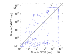
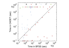
Figure 1: bfss vs Cadet: Legend: Q: QBFEval, A: Arithmetic, F: Factorization, D: Disjunctive Decomposition. TO: benchmarks for which the corresponding algorithm was unsuccessful.

bfss vs Cadet: Of the $504$ benchmarks, Cadet was successful on $231$ benchmarks, of which $24$ belonged to Disjunctive Decomposition, $22$ to Arithmetic, $1$ to Factorization and $184$ to QBFEval. Figure 1(a) gives the performance of the two algorithms with respect to time on the QBFEval suite. Here, Cadet solved $35$ benchmarks that bfss could not solve, whereas bfss solved $21$ benchmarks that could not be solved by Cadet. Figure 1(b) gives the performance of the two algorithms with respect to time on the Arithmetic, Factorization and Disjunctive Decomposition benchmarks. In these categories, there were a total of $62$ benchmarks that bfss solved that Cadet could not solve, and there was $1$ benchmark that Cadet solved but bfss did not solve. While Cadet takes less time on Arithmetic benchmarks and many QBFEval benchmarks, on Disjunctive Decomposition and Factorization, bfss takes less time.

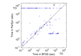
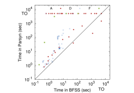
Figure 2: bfss vs parSyn (for legend see Figure 1)

bfss  vs parSyn: Figure 2 shows the comparison of time taken by bfss and parSyn. parSyn was successful on a total of $185$ benchmarks, and could solve $1$ benchmark which bfss could not solve. On the other hand, bfss solved $94$ benchmarks that parSyn could not solve. From Figure 2, we can see that on most of the Arithmetic, Disjunctive Decomposition and Factorization benchmarks, bfss takes less time than parSyn.

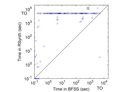
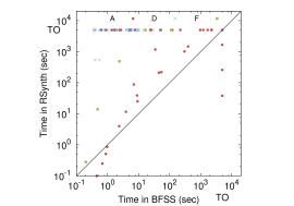
Figure 3: bfss vs RSynth (for legend see Figure 1)

bfss vs RSynth: We next compare the performance of bfss with RSynth. As shown in Figure 3, RSynth was successful on $51$ benchmarks, with $4$ benchmarks that could be solved by RSynth but not by bfss. In contrast, bfss could solve $231$ benchmarks that RSynth could not solve! Of the benchmarks that were solved by both solvers, we can see that bfss took less time on most of them.

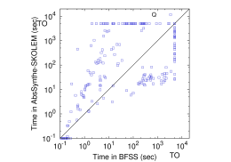
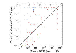
Figure 4: bfss vs AbsSynthe-Skolem (for legend see Figure 1)

bfss vs AbsSynthe-Skolem: AbsSynthe-Skolem was successful on $217$ benchmarks, and could solve $31$ benchmarks that bfss could not solve. In contrast, bfss solved a total of $92$ benchmarks that AbsSynthe-Skolem could not. Figure 4 shows a comparison of running times of bfss and AbsSynthe-Skolem.

7 Conclusion

In this paper, we showed some complexity-theoretic hardness results for the Boolean functional synthesis problem. We then developed a two-phase approach to solve this problem, where the first phase, which is an efficient algorithm generating poly-sized functions surprisingly succeeds in solving a large number of benchmarks. To explain this, we identified sufficient conditions when phase 1 gives the correct answer. For the remaining benchmarks, we employed the second phase of the algorithm that uses a CEGAR-based approach and builds Skolem functions by exploiting recent advances in SAT solvers/approximate counters. As future work, we wish to explore further improvements in Phase 2, and other structural restrictions on the input that ensure completeness of Phase 1.

Acknowledgements:

We are thankful to Ajith John, Kuldeep Meel, Mate Soos, Ocan Sankur, Lucas Martinelli Tabajara and Markus Rabe for useful discussions and for providing us with various software tools used in the experimental comparisons. We also thank the anonymous reviewers for insightful comments.

Appendix 0.A Detailed Results for individual pipelines of BFSS

As mentioned in section 6, bfss is an ensemble of two pipelines, an AIG-NNF pipeline and a BDD-wDNNF pipeline. These two pipelines accept the same input specification but represent them in two different ways. The first pipeline takes the input formula as an AIG and builds an NNF (not necessarily a wDNNF) DAG, while the second pipeline first builds an ROBDD from the input AIG using dynamic variable reordering, and then obtains a wDNNF representation from the ROBDD using the linear-time algorithm described in [14]. Once the NNF/wDNNF representation is built, the same algorithm is used to generate skolem functions, namely, Algorithm  1 is used in Phase 1 and CEGAR-based synthesis using UniGen[11] to sample counterexamples is used in Phase 2. In this section, we give the individual results of the two pipelines.

0.A.1 Performance of the AIG-NNF pipeline

Benchmark	Total	# Benchmarks	Phase 1	Phase 2	Solved By
Domain	Benchmarks	Solved	Solved	Started	Phase 2
QBFEval	383	133	122	110	11
Arithmetic	48	31	31	12	0
Disjunctive
Decomposition	68	68	66	2	2
Factorization	5	4	0	5	4

Table 2: bfss: Performance Summary for AIG-NNF pipeline

In the AIG-NNF pipeline, bfss solves a total of $236$ benchmarks, with $133$ benchmarks in QBFEval, $31$ in Arithmetic, all the $68$ benchmarks of Disjunctive Decomposition and $4$ benchmarks in Factorization. Of the $254$ benchmarks in QBFEval (as mentioned in Section 6, we could not build succinct AIGs for the remaining benchmarks and did not run our tool on them), Phase 1 solved $122$ benchmarks and Phase 2 was started on $110$ benchmarks, of which $11$ benchmarks reached completion. Of the $48$ benchmarks in Arithmetic, Phase 1 solved $31$ and Phase $2$ was started on $12$. On the remaining $5$ Arithmetic benchmarks, Phase 1 did not reach completion. Of the $68$ Disjunctive Decomposition benchmarks, $66$ were successfully solved by Phase 1 and the remaining $2$ by Phase 2. Phase 2 had started on all the $5$ benchmarks in Factorization and reached completion on $4$ benchmarks.

0.A.1.1 Plots for the AIG-NNF pipeline

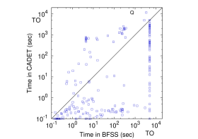
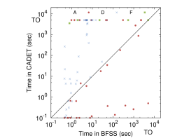
Figure 5: bfss (AIG-NNF Pipeline) vs Cadet. Legend : A: Arithmetic, F: Factorization, D: Disjunctive decomposition Q QBFEval. TO: benchmarks for which the corresponding algorithm was unsuccessful.

Figure 5 shows the performance of bfss (AIG-NNF pipeline) versus Cadet for all the four benchmark domains. Amongst the four domains, Cadet solved $53$ benchmarks that bfss could not solve. Of these, $52$ belonged to QBFEval and $1$ belonged to Arithmetic. On the other hand, bfss solved $58$ benchmarks that Cadet could not solve. Of these, $1$ belonged to QBFEval, $10$ to Arithmetic, $3$ to Factorization and $44$ to Disjunctive Decomposition. From Figure 5, we can see that while Cadet takes less time than bfss on many Arithmetic and QBFEval benchmarks, on Disjunctive Decomposition and Factorization, the AIG-NNF pipeline of bfss takes less time.

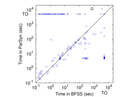
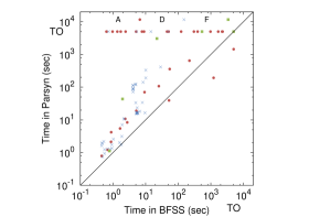
Figure 6: bfss (AIG-NNF Pipeline) vs parSyn (for legend see Figure 5)

Figure 6 shows the performance of bfss (AIG-NNF pipeline) versus parSyn. Amongst the $4$ domains, parSyn solved $22$ benchmarks that bfss could not solve, of these $1$ benchmark belonged to the Arithmetic domain and $21$ benchmarks belonged to QBFEval. On the other hand, bfss solved $73$ benchmarks that parSyn could not solve. Of these, $51$ belonged to QBFEval, $17$ to Arithmetic and $4$ to Disjunctive Decomposition. From 5, we can see that while the behaviour of parSyn and bfss is comparable for many QBFEval benchmarks, on most of the Arithmetic, Disjunctive Decomposition and Factorization benchmarks, the AIG-NNF pipeline of bfss takes less time.

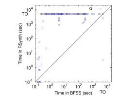
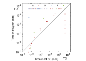
Figure 7: bfss (AIG-NNF Pipeline) vs RSynth (for legend see Figure 5)

Figure 7 gives the comparison of the AIG-NNF pipeline of bfss and RSynth. While RSynth solves $8$ benchmarks that bfss does not solve, bfss solves $193$ benchmarks that RSynth could not solve. Of these $106$ belonged to QBFEval, $20$ to Arithmetic, $66$ to Disjunctive Decomposition and $1$ to Factorization. Moreover, on most of the benchmarks that both the tools solved, bfss takes less time.

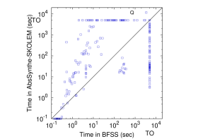
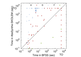
Figure 8: bfss (AIG-NNF Pipeline) vs AbsSynthe-Skolem (for legend see Figure 5)

Figure 8 gives the comparison of of the performance of the AIG-NNF pipeline of bfss and AbsSynthe-Skolem. While AbsSynthe-Skolem solves $72$ benchmarks that bfss could not solve, bfss solved $91$ benchmarks that AbsSynthe-Skolem could not solve. Of these $44$ belonged to QBFEval, $8$ to Arithmetic and $39$ to Disjunctive Decomposition.

0.A.2 Performance of the BDD-wDNNF pipeline

In this section, we discuss the performance of the BDD-wDNNF pipeline of bfss. Recall that in this pipeline the tool builds an ROBDD from the input AIG using dynamic variable reordering and then converts the ROBDD in a wDNNF representation. In this section, by bfss we mean, the BDD-wDNNF pipeline of the tool.

Table 3 gives the performance summary of the BDD-wDNNF pipeline. Using this pipeline, the tool solved a total of $230$ benchmarks, of which $143$ belonged to QBFEval, $23$ belonged to Arithmetic, $59$ belonged to Disjunctive Decomposition and $5$ belonged to Factorization. As expected, since the representation is already in wDNNF, the skolem functions generated at end of Phase 1 were indeed exact (see Theorem 4.1(b)) and we did not require to start Phase 2 on any benchmark. We also found that the memory requirements of this pipeline were higher, and for some benchmarks the tool failed because the ROBDDs (and hence resulting wDNNF representation) were large in size, resulting in out of memory errors or assertion failures in the underlying AIG library.

Benchmark	Total	# Benchmarks	Phase 1	Phase 2	Solved By
Domain	Benchmarks	Solved	Solved	Started	Phase 2
QBFEval	383	143	143	0	0
Arithmetic	48	23	23	0	0
Disjunctive
Decomposition	68	59	59	0	0
Factorization	5	5	5	0	0

Table 3: bfss: Performance Summary

0.A.2.1 Plots for the BDD-wDNNF pipeline

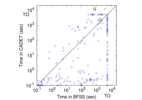
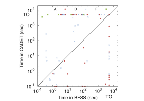
Figure 9: bfss (BDD-wDNNF Pipeline) vs Cadet (for legend see Figure 5)

Figure 5 gives the performance of bfss versus Cadet. The performance of Cadet and bfss is comparable, with Cadet solving $74$ benchmarks across all domains that bfss could not and bfss solving $73$ benchmarks that Cadet could not. While Cadet takes less time on many QBFEval benchmarks, on many Arithmetic, Disjunctive Decomposition and Factorization Benchmarks, the BDD-wDNNF pipeline of bfss takes less time.

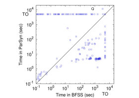
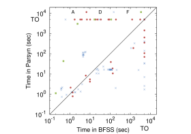
Figure 10: bfss (BDD-wDNNF Pipeline)vs parSyn (for legend see Figure 5)

Figure 10 gives the performance of bfss versus parSyn. While parSyn could solve $30$ benchmarks across all domains that bfss could not, the BDD-wDNNF pipeline of bfss solved $75$ benchmarks that parSyn could not.

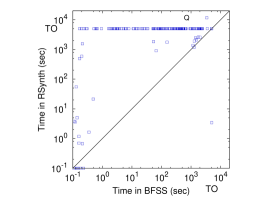
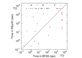
Figure 11: bfss (BDD-wDNNF Pipeline) vs RSynth (for legend see Figure 5)

Figure 11 gives the performance of bfss versus RSynth. While RSynth could solve $9$ benchmarks across all domains that bfss could not, the BDD-wDNNF pipeline of bfss solved $188$ benchmarks that RSynth could not. Furthermore from Figure 11, we can see that on most benchmarks, which both the tools could solve, bfss takes less time.

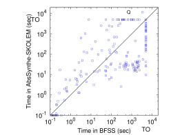
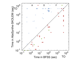
Figure 12: bfss (BDD-wDNNF Pipeline) vs AbsSynthe-Skolem (for legend see Figure 5)

Figure 12 gives the performance of bfss versus AbsSynthe-Skolem. While AbsSynthe-Skolem could solve $39$ benchmarks across all domains that bfss could not, the BDD-wDNNF pipeline of bfss solved $52$ benchmarks which could not be solved by AbsSynthe-Skolem.

0.A.3 Comparison of the two pipelines

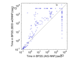
Figure 13: bfss (AIG-NNF) vs bfss (BDD-wDNNF) (for legend see Figure 5)

Figure 13 compares the performances of the two pipelines. We can see that while there were some benchmarks which only one of the pipelines could solve, apart from Factorization benchmarks, for most of the QBFEval, Arithmetic and Disjunctive Decomposition Benchmarks, the time taken by the AIG-NNF pipeline was less than the time taken by the BDD-wDNNF pipeline.

References

- [1] Website for CAV 2018 Experiments. {https://drive.google.com/drive/folders/0B74xgF9hCly5QXctNFpYR0VnQUU?usp=sharing} (2018)
- [2] Akshay, S., Chakraborty, S., John, A.K., Shah, S.: Towards parallel boolean functional synthesis. In: TACAS 2017 Proceedings, Part I. pp. 337–353 (2017), https://doi.org/10.1007/978-3-662-54577-5_19
- [3] Alur, R., Madhusudan, P., Nam, W.: Symbolic computational techniques for solving games. STTT 7(2), 118–128 (2005)
- [4] Andersson, G., Bjesse, P., Cook, B., Hanna, Z.: A proof engine approach to solving combinational design automation problems. In: Proceedings of the 39th Annual Design Automation Conference. pp. 725–730. DAC ’02, ACM, New York, NY, USA (2002), http://doi.acm.org/10.1145/513918.514101
- [5] Baader, F.: On the complexity of boolean unification. Tech. rep. (1999)
- [6] Balabanov, V., Jiang, J.H.R.: Unified qbf certification and its applications. Form. Methods Syst. Des. 41(1), 45–65 (Aug 2012), http://dx.doi.org/10.1007/s10703-012-0152-6
- [7] Boole, G.: The Mathematical Analysis of Logic. Philosophical Library (1847), https://books.google.co.in/books?id=zv4YAQAAIAAJ
- [8] Boudet, A., Jouannaud, J.P., Schmidt-Schauss, M.: Unification in boolean rings and abelian groups. J. Symb. Comput. 8(5), 449–477 (Nov 1989), http://dx.doi.org/10.1016/S0747-7171(89)80054-9
- [9] Brenguier, R., Pérez, G.A., Raskin, J.F., Sankur, O.: Abssynthe: abstract synthesis from succinct safety specifications. In: Proceedings 3rd Workshop on Synthesis (SYNT’14). Electronic Proceedings in Theoretical Computer Science, vol. 157, pp. 100–116. Open Publishing Association (2014), http://arxiv.org/abs/1407.5961v1
- [10] Bryant, R.E.: Graph-based algorithms for boolean function manipulation. IEEE Trans. Comput. 35(8), 677–691 (Aug 1986), http://dx.doi.org/10.1109/TC.1986.1676819
- [11] Chakraborty, S., Fremont, D.J., Meel, K.S., Seshia, S.A., Vardi, M.Y.: On parallel scalable uniform SAT witness generation. In: Tools and Algorithms for the Construction and Analysis of Systems - 21st International Conference, TACAS 2015, Held as Part of the European Joint Conferences on Theory and Practice of Software, ETAPS 2015, London, UK, April 11-18, 2015. Proceedings. pp. 304–319 (2015)
- [12] Chakraborty, S., Meel, K.S., Vardi, M.Y.: Algorithmic improvements in approximate counting for probabilistic inference: From linear to logarithmic SAT calls. In: Proceedings of the Twenty-Fifth International Joint Conference on Artificial Intelligence, IJCAI 2016, New York, NY, USA, 9-15 July 2016. pp. 3569–3576 (2016)
- [13] Chen, Y., Eickmeyer, K., Flum, J.: The exponential time hypothesis and the parameterized clique problem. In: Proceedings of the 7th International Conference on Parameterized and Exact Computation. pp. 13–24. IPEC’12, Springer-Verlag, Berlin, Heidelberg (2012)
- [14] Darwiche, A.: Decomposable negation normal form. J. ACM 48(4), 608–647 (2001)
- [15] Deschamps, J.P.: Parametric solutions of boolean equations. Discrete Math. 3(4), 333–342 (Jan 1972), http://dx.doi.org/10.1016/0012-365X(72)90090-8
- [16] Fried, D., Tabajara, L.M., Vardi, M.Y.: BDD-based boolean functional synthesis. In: Computer Aided Verification - 28th International Conference, CAV 2016, Toronto, ON, Canada, July 17-23, 2016, Proceedings, Part II. pp. 402–421 (2016)
- [17] IP01: On the complexity of k-sat. J. Comput. Syst. Sci. 62(2), 367–375 (2001)
- [18] Jacobs, S., Bloem, R., Brenguier, R., Könighofer, R., Pérez, G.A., Raskin, J., Ryzhyk, L., Sankur, O., Seidl, M., Tentrup, L., Walker, A.: The second reactive synthesis competition (SYNTCOMP 2015). In: Proceedings Fourth Workshop on Synthesis, SYNT 2015, San Francisco, CA, USA, 18th July 2015. pp. 27–57 (2015)
- [19] Jiang, J.H.R.: Quantifier elimination via functional composition. In: Proc. of CAV. pp. 383–397. Springer (2009)
- [20] Jiang, J.H.R., Balabanov, V.: Resolution proofs and Skolem functions in QBF evaluation and applications. In: Proc. of CAV. pp. 149–164. Springer (2011)
- [21] Jo, S., Matsumoto, T., Fujita, M.: Sat-based automatic rectification and debugging of combinational circuits with lut insertions. In: Proceedings of the 2012 IEEE 21st Asian Test Symposium. pp. 19–24. ATS ’12, IEEE Computer Society (2012)
- [22] John, A., Shah, S., Chakraborty, S., Trivedi, A., Akshay, S.: Skolem functions for factored formulas. In: FMCAD. pp. 73–80 (2015)
- [23] Karp, R., Lipton, R.: Turing machines that take advice. L’Enseignment Math/’ematique 28(2), 191–209 (1982)
- [24] Kuehlmann, A., Paruthi, V., Krohm, F., Ganai, M.K.: Robust boolean reasoning for equivalence checking and functional property verification. IEEE Trans. on CAD of Integrated Circuits and Systems 21(12), 1377–1394 (2002), http://dblp.uni-trier.de/db/journals/tcad/tcad21.html#KuehlmannPKG02
- [25] Kuncak, V., Mayer, M., Piskac, R., Suter, P.: Complete functional synthesis. SIGPLAN Not. 45(6), 316–329 (Jun 2010)
- [26] Logic, B., Group, V.: ABC: A System for Sequential Synthesis and Verification . http://www.eecs.berkeley.edu/~alanmi/abc/
- [27] Lowenheim, L.: Über die Auflösung von Gleichungen in Logischen Gebietkalkul. Math. Ann. 68, 169–207 (1910)
- [28] Macii, E., Odasso, G., Poncino, M.: Comparing different boolean unification algorithms. In: Proc. of 32nd Asilomar Conference on Signals, Systems and Computers. pp. 17–29 (2006)
- [29] Marijn Heule, M.S., Biere, A.: Efficient Extraction of Skolem Functions from QRAT Proofs. In: Formal Methods in Computer-Aided Design, FMCAD 2014, Lausanne, Switzerland, October 21-24, 2014. pp. 107–114 (2014)
- [30] Martin, U., Nipkow, T.: Boolean unification - the story so far. J. Symb. Comput. 7(3-4), 275–293 (Mar 1989), http://dx.doi.org/10.1016/S0747-7171(89)80013-6
- [31] Niemetz, A., Preiner, M., Lonsing, F., Seidl, M., Biere, A.: Resolution-based certificate extraction for QBF - (tool presentation). In: Theory and Applications of Satisfiability Testing - SAT 2012 - 15th International Conference, Trento, Italy, June 17-20, 2012. Proceedings. pp. 430–435 (2012)
- [32] QBFLib: Qbfeval 2017. http://www.qbflib.org/event_page.php?year=2017
- [33] Rabe, M.N., Seshia, S.A.: Incremental determinization. In: Theory and Applications of Satisfiability Testing - SAT 2016 - 19th International Conference, Bordeaux, France, July 5-8, 2016, Proceedings. pp. 375–392 (2016), https://doi.org/10.1007/978-3-319-40970-2_23
- [34] Rabe, M.N., Tentrup, L.: CAQE: A certifying QBF solver. In: Formal Methods in Computer-Aided Design, FMCAD 2015, Austin, Texas, USA, September 27-30, 2015. pp. 136–143 (2015)
- [35] Rabe, M.N., Seshia, S.A.: Incremental determinization. In: Theory and Applications of Satisfiability Testing - SAT 2016 - 19th International Conference, Bordeaux, France, July 5-8, 2016, Proceedings. pp. 375–392 (2016), https://doi.org/10.1007/978-3-319-40970-2_23
- [36] Solar-Lezama, A.: Program sketching. STTT 15(5-6), 475–495 (2013)
- [37] Solar-Lezama, A., Rabbah, R.M., Bodík, R., Ebcioglu, K.: Programming by sketching for bit-streaming programs. In: Proceedings of the ACM SIGPLAN 2005 Conference on Programming Language Design and Implementation, Chicago, IL, USA, June 12-15, 2005. pp. 281–294 (2005)
- [38] Srivastava, S., Gulwani, S., Foster, J.S.: Template-based program verification and program synthesis. STTT 15(5-6), 497–518 (2013)
- [39] Tabajara, L.M., Vardi, M.Y.: Factored boolean functional synthesis. In: 2017 Formal Methods in Computer Aided Design, FMCAD 2017, Vienna, Austria, October 2-6, 2017. pp. 124–131 (2017)
- [40] Trivedi, A.: Techniques in Symbolic Model Checking. Master’s thesis, Indian Institute of Technology Bombay, Mumbai, India (2003)
- [41] Zhu, S., Tabajara, L.M., Li, J., Pu, G., Vardi, M.Y.: Symbolic LTLf synthesis. In: Proceedings of the Twenty-Sixth International Joint Conference on Artificial Intelligence, IJCAI 2017, Melbourne, Australia, August 19-25, 2017. pp. 1362–1369 (2017)