Fast solvers for two-dimensional fractional diffusion equations using rank structured matrices

Abstract

We consider the discretization of time-space diffusion equations with fractional derivatives in space and either one-dimensional (1D) or 2D spatial domains. The use of an implicit Euler scheme in time and finite differences or finite elements in space leads to a sequence of dense large scale linear systems describing the behavior of the solution over a time interval. We prove that the coefficient matrices arising in the 1D context are rank structured and can be efficiently represented using hierarchical formats ($\mathcal{H}$-matrices, HODLR). Quantitative estimates for the rank of the off-diagonal blocks of these matrices are presented. We analyze the use of HODLR arithmetic for solving the 1D case and we compare this strategy with existing methods that exploit the Toeplitz-like structure to precondition the GMRES iteration. The numerical tests demonstrate the convenience of the HODLR format when at least a reasonably low number of time steps is needed. Finally, we explain how these properties can be leveraged to design fast solvers for problems with 2D spatial domains that can be reformulated as matrix equations. The experiments show that the approach based on the use of rank-structured arithmetic is particularly effective and outperforms current state of the art techniques.

35R11, 15A24, 65F10.

1 Introduction

Fractional Diffusion Equations (FDEs) are a generalization of the classical partial diffusion equations obtained by replacing a standard derivative with a fractional one. In the last decade, FDEs have gained a lot of attention since they allow to model non-local behavior, e.g., enhanced diffusivity, which can be regarded as a realistic representation of specific physical phenomena appearing in several applications. In finance, this is used to take long time correlations into consideration [40]; in image processing, the use of fractional anisotropic diffusion allows to accurately recover images from their corrupted or noisy version — without incurring the risks of over-regularizing the solution and thus losing significant part of the image such as the edges [2]. The applications in fusion plasma physics concern Tokamak reactors (like ITER currently under construction in the South of France [1]) which are magnetic toroidal confinement devices aiming to harvest energy from the fusion of small atomic nuclei, typically Deuterium and Tritium, heated to the plasma state. Recent experimental and theoretical evidence indicates that transport in Tokamak reactors deviates from the standard diffusion paradigm. One of the proposed models that incorporates in a natural, unified way, the unexpected anomalous diffusion phenomena is based on the use of fractional derivative operators [10]. The development of fast numerical tools for solving the resulting equations is then a key requirement for controlled thermonuclear fusion, which offers the possibility of clean, sustainable, and almost limitless energy.

Let us briefly recall how a standard diffusion equation can be “fractionalized”, by taking as an example the parabolic diffusion equation $\frac{\partial u(x,t)}{\partial t}=~{}d(x,t)\frac{\partial^{2}u(x,t)}{\partial x^{2}}$, where $d(x,t)$ is the diffusion coefficient. Replacing the derivative in time with a fractional one leads to a time-fractional diffusion equation; in this case, the fractional derivative order is chosen between $0$ and $1$. On the other hand, we can consider a space-fractional diffusion equation by introducing a fractional derivative in space, with order between $1$ and $2$. The two approaches (which can also be combined), lead to similar computational issues. In this paper, we focus on the space fractional initial-boundary value problem

(4) $$\left\{\begin{array}[]{lc}\frac{\partial u(x,t)}{\partial t}=d_{+}(x,t)\frac{\partial^{\alpha}u(x,t)}{\partial_{+}x^{\alpha}}+d_{-}(x,t)\frac{\partial^{\alpha}u(x,t)}{\partial_{-}x^{\alpha}}+f(x,t),&(x,t)\in(L,R)\times(0,T],\\ u(x,t)=u(x,t)=0,&(x,t)\in\mathbb{R}\backslash(L,R)\times[0,T],\\ u(x,0)=u_{0}(x),&x\in[L,R],\end{array}\right.$$

where $\alpha\in(1,2)$ is the fractional derivative order, $f(x,t)$ is the source term, and the nonnegative functions $d_{\pm}(x,t)$ are the diffusion coefficients. Three of the most famous definitions of the right-handed (–) and the left-handed (+) fractional derivatives in (4) are due to Riemann–Liouville, Caputo, and Grünwald-Letnikov. We refer the reader to Section 2 for a detailed discussion.

As suggested in [11], in order to guarantee the well-posedness of a space-FDE problem, the value of the solution on $\mathbb{R}\backslash(L,R)$ must be properly accounted for. In this view, in (4) we fix the so-called absorbing boundary conditions, that is we assume that the particles are “killed” whenever they leave the domain $(L,R)$.

Analogously, one can generalize high dimensional differential operators by applying (possibly different order) fractional derivatives in each coordinate direction. More explicitly, we consider the 2D extension of (4)

(5) $$\begin{split}\frac{\partial u(x,y,,t)}{\partial t}&=d_{1,+}(x,t)\frac{\partial^{\alpha_{1}}u(x,y,t)}{\partial_{+}x^{\alpha_{1}}}+d_{1,-}(x,t)\frac{\partial^{\alpha_{1}}u(x,y,t)}{\partial_{-}x^{\alpha_{1}}}\\ &+d_{2,+}(y,t)\frac{\partial^{\alpha_{2}}u(x,y,t)}{\partial_{+}y^{\alpha_{2}}}+d_{2,-}(y,t)\frac{\partial^{\alpha_{2}}u(x,y,t)}{\partial_{-}y^{\alpha_{2}}}+f(x,y,t).\end{split}$$

with absorbing boundary conditions. Notice that the diffusion coefficients only depend on time and on the variable of the corresponding differential operator. This choice makes it easier to treat a 2D FDE problem as a matrix equation and to design fast numerical procedures for it (see Section 4).

1.1 Existing numerical methods for FDE problems

The non-local nature of fractional differential operators causes the absence of sparsity in the coefficient matrix of the corresponding discretized problem. This makes FDEs computationally more demanding than PDEs.

Various numerical discretization methods for FDE problems, e.g., finite differences, finite volumes, finite elements have been the subject of many studies [34, 45, 15]. In the case of regular spatial domains, the discretization matrices often inherit a Toeplitz-like structure from the space-invariant property of the underlying operators. Iterative schemes such as multigrid and preconditioned Krylov methods — able to exploit this structure — can be found in [50, 29, 38, 26, 37, 36, 12, 35]. For both one- and two-dimensional FDE problems, we mention the structure preserving preconditioning and the algebraic multigrid methods presented in [12, 35]. Both strategies are based on the spectral analysis of the coefficient matrices via their spectral symbol. The latter is a function which provides a compact spectral description of the discretization matrices whose computation relies on the theory of Generalized Locally Toeplitz (GLT) matrix-sequences [18].

Only very recently, off-diagonal rank structures have been recognized in finite element discretizations [52]. Indeed, Zhao et al. proposed the use of hierarchical matrices for storing the stiffness matrix combined with geometric multigrid (GMG) for solving the linear system.

It is often the case that 2D problems with piecewise smooth right-hand sides have piecewise smooth solutions (see, e.g., [9]). A possible way to uncover and leverage this property is to rephrase the linear system in matrix equation form. This is done for instance in [8], where the authors use the Toeplitz-like structure of the involved one-dimensional FDE matrices in combination with the extended Krylov subspace method to deal with fine discretizations.

1.2 Motivation and contribution

In this paper, we aim to build a framework for analyzing the low-rank properties of one-dimensional FDE discretizations and to design fast algorithms for solving two-dimensional FDEs written in a matrix equation form. In detail, the piecewise smooth property of the right-hand side implies the low-rank structure in the solution of the matrix equation and enables the use of Krylov subspace methods [8]. This, combined with the technology of hierarchically rank-structured matrices such as $\mathcal{H}$-matrices and HODLR [24], yields a linear-polylogarithmic computational complexity in the size of the edge of the mesh. For instance, for a $N\times N$ grid we get a linear polylogarithmic cost in $N$, in contrast to $\mathcal{O}(N^{2}\log N)$ needed by a multigrid approach or a preconditioned iterative method applied to linear systems with dense Toeplitz coefficient matrices. Similarly, the storage consumption is reduced from $\mathcal{O}(N^{2})$ to $\mathcal{O}(N\log N)$. The numerical experiments demonstrate that our approach, based on the HODLR format, outperforms the one proposed in [8], although the asymptotic cost is comparable. From the theoretical side, we provide an analysis of the rank structure in the matrices coming from the discretization of fractional differential operators. Our main results claim that the off-diagonal blocks in these matrices have numerical rank $\mathcal{O}(\log(\epsilon^{-1})\log(N))$ where $\epsilon$ is the truncation threshold. We highlight that some of these results do not rely on the Toeplitz structure and apply to more general cases, e.g., stiffness matrices of finite element methods on non-uniform meshes.

The use of hierarchical matrices for finite element discretization of FDEs has already been explored in the literature. For instance, the point of view in [52] is similar to the one we take in Section 3.3; however, we wish to highlight two main differences with our contribution. First, Zhao et al. considered the adaptive geometrically balanced clustering [21], in place of the HODLR partitioning. As mentioned in the Section 3.4.3, there is only little difference between the off-diagonal ranks of the two partitionings, hence HODLR arithmetic turns out to be preferable because it reduces the storage consumption. Second, they propose the use of geometric multigrid (GMG) for solving linear systems with the stiffness matrix. In the case of multiple time steps and for generating the extended Krylov subspace, precomputing the LU factorization is more convenient, as we discuss in Section 5. To the best of our knowledge, the rank structure in finite difference discretizations of fractional differential operators has not been previously noticed.

The paper is organized as follows; in Section 2 we recall different definitions of fractional derivatives and the discretizations proposed in the literature. Section 3 is dedicated to the study of the rank structure arising in the discretizations. More specifically, in Section 3.1 a preliminary qualitative analysis is supported by the GLT theory, providing a decomposition of each off-diagonal block as the sum of a low-rank plus a small-norm term. Then, a quantitative analysis is performed in Sections 3.2 and 3.3, with different techniques stemming from the framework of structured matrices. In Section 3.4 we introduce the HODLR format and we discuss how to efficiently construct representations of the matrices of interest. Section 3.5 briefly explains how to combine these ingredients to solve the 1D problem. In Section 4 we reformulate the 2D problem as a Sylvester matrix equation with structured coefficients and we illustrate a fast solver. The performances of our approach are tested and compared in Section 5. Conclusion and future outlook are given in Section 6.

2 Fractional derivatives and their discretizations

2.1 Definitions of fractional derivatives

A common definition of fractional derivatives is given by the Riemann–Liouville formula. For a given function with absolutely continuous first derivative on $[L,R]$, the right-handed and left-handed Riemann–Liouville fractional derivatives of order $\alpha$ are defined by

(6) $$\begin{split}\frac{\partial^{\alpha}u(x,t)}{\partial^{RL}_{+}x^{\alpha}}&=\frac{1}{\Gamma(n-\alpha)}\frac{\partial^{n}}{\partial x^{n}}\int_{L}^{x}\frac{u(\xi,t)}{(x-\xi)^{\alpha+1-n}}d\xi,\\ \frac{\partial^{\alpha}u(x,t)}{\partial^{RL}_{-}x^{\alpha}}&=\frac{(-1)^{n}}{\Gamma(n-\alpha)}\frac{\partial^{n}}{\partial x^{n}}\int_{x}^{R}\frac{u(\xi,t)}{(\xi-x)^{\alpha+1-n}}d\xi,\end{split}$$

where $n$ is the integer such that $n-1<\alpha\leqslant n$ and $\Gamma(\cdot)$ is the Euler gamma function. Note that the left–handed fractional derivative of the function $u(x,t)$ computed at $x$ depends on all function values to the left of $x$, while the right–handed fractional derivative depends on the ones to the right.

When $\alpha=m$, with $m\in\mathbb{N}$, then (6) reduces to the standard integer derivatives, i.e.,

$$\frac{\partial^{m}u(x,t)}{\partial^{RL}_{+}x^{m}}=\frac{\partial^{m}u(x,t)}{\partial x^{m}},\quad\frac{\partial^{m}u(x,t)}{\partial^{RL}_{-}x^{m}}=(-1)^{m}\frac{\partial^{m}u(x,t)}{\partial x^{m}}.$$

An alternative definition is based on the Grünwald–Letnikov formulas:

(7) $$\begin{split}\frac{\partial^{\alpha}u(x,t)}{\partial^{GL}_{+}x^{\alpha}}&=\lim_{\Delta x\rightarrow 0^{+}}\frac{1}{\Delta x^{\alpha}}\sum_{k=0}^{\lfloor(x-L)/\Delta x\rfloor}g_{k}^{(\alpha)}u(x-k\Delta x,t),\\ \frac{\partial^{\alpha}u(x,t)}{\partial^{GL}_{-}x^{\alpha}}&=\lim_{\Delta x\rightarrow 0^{+}}\frac{1}{\Delta x^{\alpha}}\sum_{k=0}^{\lfloor(R-x)/\Delta x\rfloor}g_{k}^{(\alpha)}u(x+k\Delta x,t),\end{split}$$

where $\lfloor\cdot\rfloor$ is the floor function, $g_{k}^{(\alpha)}$ are the alternating fractional binomial coefficients

$$g_{k}^{(\alpha)}=(-1)^{k}\binom{\alpha}{k}=\frac{(-1)^{k}}{k!}\alpha(\alpha-1)\cdots(\alpha-k+1)\qquad k=1,2,\ldots$$

and $g_{0}^{(\alpha)}=1$. Formula (7) can be seen as an extension of the definition of ordinary derivatives via limit of the difference quotient.

Finally, another common definition of fractional derivative was proposed by Caputo:

(8) $$\begin{split}\frac{\partial^{\alpha}u(x,t)}{\partial^{C}_{+}x^{\alpha}}&=\frac{1}{\Gamma(n-\alpha)}\int_{L}^{x}\frac{\frac{\partial^{n}}{\partial\xi^{n}}u(\xi,t)}{(x-\xi)^{\alpha+1-n}}d\xi,\\ \frac{\partial^{\alpha}u(x,t)}{\partial^{C}_{-}x^{\alpha}}&=\frac{(-1)^{n}}{\Gamma(n-\alpha)}\int_{x}^{R}\frac{\frac{\partial^{n}}{\partial\xi^{n}}u(\xi,t)}{(\xi-x)^{\alpha+1-n}}d\xi.\end{split}$$

Note that (8) requires the $n$th derivative of $u(x,t)$ to be absolutely integrable. Higher regularity of the solution is typically imposed in time rather than in space; as a consequence, the Caputo formulation is mainly used for fractional derivatives in time, while Riemann–Liouville’s is preferred for fractional derivatives in space. The use of Caputo’s derivative provides some advantages in the treatment of boundary conditions when applying the Laplace transform method (see [39, Chapter 2.8]).

The various definitions are equivalent only if $u(x,t)$ is sufficiently regular and/or vanishes with all its derivatives on the boundary. In detail, it holds that:

• if the $n$th space derivative of $u(x,t)$ is continuous on $[L,R]$, then

  $$\frac{\partial^{\alpha}u(x,t)}{\partial^{RL}_{+}x^{\alpha}}=\frac{\partial^{\alpha}u(x,t)}{\partial^{GL}_{+}x^{\alpha}},\qquad\frac{\partial^{\alpha}u(x,t)}{\partial^{RL}_{-}x^{\alpha}}=\frac{\partial^{\alpha}u(x,t)}{\partial^{GL}_{-}x^{\alpha}}.$$

• if $\frac{\partial^{\ell}}{\partial x^{\ell}}u(L,t)=\frac{\partial^{\ell}}{\partial x^{\ell}}u(R,t)=0$ for all $\ell=0,1,\dots,n-1$, then

  $$\frac{\partial^{\alpha}u(x,t)}{\partial^{RL}_{+}x^{\alpha}}=\frac{\partial^{\alpha}u(x,t)}{\partial^{C}_{+}x^{\alpha}},\qquad\frac{\partial^{\alpha}u(x,t)}{\partial^{RL}_{-}x^{\alpha}}=\frac{\partial^{\alpha}u(x,t)}{\partial^{C}_{-}x^{\alpha}};$$

In this work we are concerned with space fractional derivatives so we focus on the Riemann–Liouville and the Grünwald–Letnikov formulations. However, the analysis of the structure in the discretizations can be generalized with minor adjustments to the Caputo case.

2.2 Discretizations of fractional derivatives

We consider two different discretization schemes for the FDE problem (4): finite differences and finite elements. The first scheme relies on the Grünwald–Letnikov formulation while the second is derived adopting the Riemann–Liouville definition.

2.2.1 Finite difference scheme using Grünwald-Letnikov formulas

As suggested in [34], in order to obtain a consistent and unconditionally stable finite difference scheme for (4), we use a shifted version of the Grünwald–Letnikov fractional derivatives obtained replacing $k\Delta x$ with $(k-1)\Delta x$ in (7).

Let us fix two positive integers $N,M$, and define the following partition of $[L,R]\times[0,T]$:

(9) $$x_{i}=L+i\Delta x,\quad\Delta x=\frac{(R-L)}{N+1},\quad i=0,\ldots,N+1,$$

$$t_{m}=m\Delta t,\quad\Delta t=\frac{T}{M+1},\quad m=0,\ldots,M+1.$$

The idea in [34] is to combine a discretization in time of equation (4) by an implicit Euler method with a first order discretization in space of the fractional derivatives by a shifted Grünwald-Letnikov estimate, i.e.,

$$\frac{u(x_{i},t_{m})-u(x_{i},t_{m-1})}{\Delta t}=d_{+,i}^{(m)}\frac{\partial^{\alpha}u(x_{i},t_{m})}{\partial^{GL}_{+}x^{\alpha}}+d_{-,i}^{(m)}\frac{\partial^{\alpha}u(x_{i},t_{m})}{\partial^{GL}_{-}x^{\alpha}}+f_{i}^{(m)}+\mathcal{O}(\Delta t),$$

where $d_{\pm,i}^{(m)}=d_{\pm}(x_{i},t_{m})$, $f_{i}^{(m)}:=f(x_{i},t_{m})$ and

$$\frac{\partial^{\alpha}u(x_{i},t_{m})}{\partial^{GL}_{+}x^{\alpha}} =\frac{1}{\Delta x^{\alpha}}\sum_{k=0}^{i+1}g_{k}^{(\alpha)}u(x_{i-k+1},t_{m})+\mathcal{O}(\Delta x),$$

$$\frac{\partial^{\alpha}u(x_{i},t_{m})}{\partial^{GL}_{-}x^{\alpha}} =\frac{1}{\Delta x^{\alpha}}\sum_{k=0}^{N-i+2}g_{k}^{(\alpha)}u(x_{i+k-1},t_{m})+\mathcal{O}(\Delta x).$$

The resulting finite difference approximation scheme is then

$$\frac{u_{i}^{(m)}-u_{i}^{(m-1)}}{\Delta t}=\frac{d_{+,i}^{(m)}}{\Delta x^{\alpha}}\sum_{k=0}^{i+1}g_{k}^{(\alpha)}u_{i-k+1}^{(m)}+\frac{d_{-,i}^{(m)}}{\Delta x^{\alpha}}\sum_{k=0}^{N-i+2}g_{k}^{(\alpha)}u_{i+k-1}^{(m)}+f_{i}^{(m)},$$

where by $u_{i}^{(m)}$ we denote a numerical approximation of $u(x_{i},t_{m})$. The previous approximation scheme can be written in matrix form as (see [49])

(10) $$\mathcal{M}^{\operatorname{FD},m}_{\alpha,N}u^{(m)}=\left(I+\frac{\Delta t}{\Delta x^{\alpha}}(D_{+}^{(m)}T_{\alpha,N}+D_{-}^{(m)}T_{\alpha,N}^{T})\right)u^{(m)}=u^{(m-1)}+\Delta tf^{(m)},$$

$u^{(m)}=[u_{1}^{(m)},\ldots,u_{N}^{(m)}]^{T}$, $f^{(m)}=[f_{1}^{(m)},\ldots,f_{N}^{(m)}]^{T}$, $D_{\pm}^{(m)}={\rm diag}(d_{\pm,1}^{(m)},\ldots,d_{\pm,N}^{(m)})$, $I$ is the identity matrix of order $N$ and

(11) $$T_{\alpha,N}=-\left[\begin{matrix}g_{1}^{(\alpha)}&g_{0}^{(\alpha)}&0&\cdots&0&0\\ g_{2}^{(\alpha)}&g_{1}^{(\alpha)}&g_{0}^{(\alpha)}&0&\cdots&0\\ \vdots&\ddots&\ddots&\ddots&\ddots&\vdots\\ \vdots&\ddots&\ddots&\ddots&\ddots&0\\ g_{N-1}^{(\alpha)}&\ddots&\ddots&\ddots&g_{1}^{(\alpha)}&g_{0}^{(\alpha)}\\ g_{N}^{(\alpha)}&g_{N-1}^{(\alpha)}&\cdots&\cdots&g_{2}^{(\alpha)}&g_{1}^{(\alpha)}\end{matrix}\right]_{N\times N}$$

is a lower Hessenberg Toeplitz matrix. Note that $\mathcal{M}^{\operatorname{FD},m}_{\alpha,N}$ has a Toeplitz-like structure, in the sense that it can be expressed as a sum of products between diagonal and dense Toeplitz matrices. It can be shown that $\mathcal{M}^{\operatorname{FD},m}_{\alpha,N}$ is strictly diagonally dominant and then non singular (see [34, 49]), for every choice of the parameters $m\geqslant 0$, $N\geqslant 1$, $\alpha\in(1,2)$. Moreover, it holds $g_{1}^{(\alpha)}=-\alpha$, $g_{0}^{(\alpha)}>g_{2}^{(\alpha)}>g_{3}^{(\alpha)}>\dots>0$ and $g_{k}^{(\alpha)}=\mathcal{O}(k^{-\alpha-1})$.

2.2.2 Finite element space discretization

We consider a finite element discretization for (4), using the Riemann–Liouville formulation (6). Let $\mathcal{B}=\{\varphi_{1},\ldots,\varphi_{N}\}$ be a finite element basis, consisting of positive functions with compact support that vanish on the boundary. At each time step $t$, we replace the true solution $u$ by its finite element approximation $u_{\Delta x}$

(12) $$u_{\Delta x}=\sum_{j=1}^{N}u_{j}(t)\varphi_{j}(x),$$

then we formulate a finite element scheme for (4). Assuming that the diffusion coefficients do not depend on $t$, by means of this formulation we can find the steady-state solution solving the linear system $\mathcal{M}^{\operatorname{FE}}_{\alpha,N}u=f$, with

$$(\mathcal{M}^{\operatorname{FE}}_{\alpha,N})_{ij}=\langle\varphi_{i}(x),d_{+}(x)\frac{\partial^{\alpha}\varphi_{j}(x)}{\partial^{RL}_{+}x^{\alpha}}+d_{-}(x)\frac{\partial^{\alpha}\varphi_{j}(x)}{\partial^{RL}_{-}x^{\alpha}}\rangle,\qquad f_{i}=\langle-v(x),\varphi_{i}(x)\rangle.$$

By linearity, we can decompose $\mathcal{M}^{\operatorname{FE}}_{\alpha,N}=\mathcal{M}^{\operatorname{FE},+}_{\alpha,N}+\mathcal{M}^{\operatorname{FE},-}_{\alpha,N}$ where $\mathcal{M}^{\operatorname{FE},+}_{\alpha,N}$ includes the action of the left-handed derivative, and $\mathcal{M}^{\operatorname{FE},-}_{\alpha,N}$ the effect of the right-handed one.

The original time-dependent equation (4) can be solved by means of a suitable time discretization (such as the implicit Euler method used in the previous section) combined with the finite element scheme introduced here (see, e.g., [13, 31]). In the time-dependent case, the matrix associated with the instant $t_{m}$ will be denoted by $\mathcal{M}^{\operatorname{FE},m}_{\alpha,N}$, and it has the same structure of $\mathcal{M}^{\operatorname{FE}}_{\alpha,N}$ up to a shift by the mass matrix $M$:

$$\mathcal{M}^{\operatorname{FE},m}_{\alpha,N}=M-\Delta t\mathcal{M}^{\operatorname{FE}}_{\alpha,N},\qquad(M)_{ij}=\langle\varphi_{i}(x),\varphi_{j}(x)\rangle.$$

The resulting time stepping scheme can be expressed as follows

$$\mathcal{M}^{\operatorname{FE},m}_{\alpha,N}u^{(m)}=Mu^{(m-1)}+\Delta tf^{(m)}.$$

We refer the reader to [15, 41] for more details on the finite element discretization of fractional problems, including a detailed analysis of the spaces used for the basis functions and convergence properties.

3 Rank structure in the 1D case

The aim of this section is to prove that different formulations of 1D fractional derivatives generate discretizations with similar properties. In particular, we are interested in showing that off-diagonal blocks in the matrix discretization of such operators have a low numerical rank. When these “off-diagonal ranks” are exact (and not just numerical ranks) this structure is sometimes called quasiseparability, or semiseparability [14, 48], see also Figure 1. Here we recall the definition and some basic properties.

Definition 3.1.

A matrix $A\in\mathbb{C}^{N\times N}$ is quasiseparable of order $k$ (or quasiseparable of rank $k$) if the maximum of the ranks of all its submatrices contained in the strictly upper or lower part is exactly $k$.

Figure 1: Pictorial description of the quasiseparable structure; the off-diagonal blocks can be represented as low-rank outer products.

Lemma 3.2.

Let $A,B\in\mathbb{C}^{N\times N}$ be quasiseparable of rank $k_{A}$ and $k_{B}$, respectively.

1. The quasiseparable rank of both $A+B$ and $A\cdot B$ is at most $k_{A}+k_{B}$.

2. If $A$ is invertible then $A^{-1}$ has quasiseparable rank $k_{A}$.

In order to perform the analysis of the off-diagonal blocks we need to formalize the concept of numerical rank. In the rest of the paper, $\lVert\cdot\rVert$ will indicate the Euclidean norm.

Definition 3.3.

We say that a matrix $X$ has $\epsilon$-rank $k$, and we write $\mathrm{rank}_{\epsilon}(X)=k$, if there exists $\delta X$ such that $\lVert\delta X\rVert\leqslant\epsilon\lVert X\rVert$, $\mathrm{rank}(X+\delta X)=k$ and the rank of $X+\delta X^{\prime}$ is at least $k$ for any other $\lVert\delta X^{\prime}\rVert\leqslant\epsilon\lVert X\rVert$. More formally:

$$\mathrm{rank}_{\epsilon}(X)=\min_{\lVert\delta X\rVert\leqslant\epsilon\lVert X\rVert}\mathrm{rank}(X+\delta X).$$

Often we are interested in measuring approximate quasiseparability. We can give a similar “approximate” definition.

Definition 3.4.

We say that a matrix $X$ has $\epsilon$-qsrank $k$ if for any off-diagonal block $Y$ of $X$ there exists a perturbation $\delta Y$ such that $\lVert\delta Y\rVert\leqslant\epsilon\lVert X\rVert$ and $Y+\delta Y$ has rank (at most) $k$. More formally:

$$\mathrm{qsrank}_{\epsilon}(X)=\max_{Y\in\mathrm{Off}(X)}\min_{\lVert\delta Y\rVert\leqslant\epsilon\lVert X\rVert}\mathrm{rank}(Y+\delta Y),$$

where $\mathrm{Off}(X)$ is the set of the off-diagonal blocks of $X$.

Remark 3.5.

As shown in [32], $\mathrm{qsrank}_{\epsilon}(X)=k$ implies the existence of a “global” perturbation $\delta X$ such that $X+\delta X$ is quasiseparable of rank $k$ and $\lVert\delta X\rVert\leqslant\epsilon\sqrt{N}$. In addition, the presence of $\lVert X\rVert$ in the above definition makes the $\epsilon$-qsrank invariant under rescaling, i.e., $\mathrm{qsrank}_{\epsilon}(A)=\mathrm{qsrank}_{\epsilon}(\theta A)$ for any $\theta\in\mathbb{C}\setminus\{0\}$.

The purpose of the following subsections is to show that the various discretizations of fractional derivatives provide matrices with small $\epsilon$-qsrank. The $\epsilon$-qsrank turns out to grow asymptotically as $\mathcal{O}(\log(\epsilon^{-1})\log(N))$, see Table 1 which summarizes our findings.

Discretization	$\epsilon$-qsrank	Reference
Finite differences	$2+2\left\lceil\frac{2}{\pi^{2}}\log\left(\frac{4}{\pi}N\right)\log\left(\frac{32}{\epsilon}\right)\right\rceil$	Lem. 3.17, Cor. 3.19
Finite elements	$k+2\left\lceil\log_{2}\left(\frac{R-L}{\delta}\right)\right\rceil\cdot\left(1+\left\lceil\log_{2}\left(\frac{(\alpha+1)\cdot 4^{\alpha+1}}{\epsilon}\right)\right\rceil\right)$	Thm. 3.27

Table 1: Bounds for the $\epsilon$-qsrank of different discretizations. For finite elements methods with equispaced basis functions the parameter $(R-L)/\delta\approx N$, and $k$ is the number of overlapping basis functions (see Definition 3.21).

3.1 Qualitative analysis of the quasiseparable structure through GLT theory

In the 1D setting the finite difference discretization matrices $\mathcal{M}^{\operatorname{FD},m}_{\alpha,N}$ present a diagonal-times-Toeplitz structure — see (10) — where the diagonal matrices are the discrete counterpart of the diffusion coefficients and the Toeplitz components come from the fractional derivatives. This structure falls in the Generalized Locally Toeplitz (GLT) class, an algebra of matrix-sequences obtained as a closure under some algebraic operations (linear combination, product, inversion, conjugation) of Toeplitz, diagonal and low-rank plus small-norm matrix-sequences.

In the remaining part of this section we show that the off-diagonal blocks of $\mathcal{M}^{\operatorname{FD},m}_{\alpha,N}$ can be decomposed as the sum of a low-rank plus a small-norm term. Such a result is obtained exploiting the properties of some simple GLT sequences, i.e., Toeplitz and Hankel sequences associated with a function $f\in L^{1}$.

Definition 3.6.

Let $f\in L^{1}([-\pi,\pi])$ and let $\left\{f_{j}\right\}_{j\in\mathbb{Z}}$ be its Fourier coefficients. Then the sequence of $N\times N$ matrices $\left\{T_{N}\right\}_{N\in\mathbb{N}}$ with $T_{N}=[f_{i-j}]_{i,j=1}^{N}$ (resp. $\{H_{N}\}_{N}$ with $H_{N}=[f_{i+j-2}]_{i,j=1}^{N}$) is called the sequence of Toeplitz (resp. Hankel) matrices generated by $f$.

The generating function $f$ provides a description of the spectrum of $T_{N}$, for $N$ large enough in the sense of the following definition.

Definition 3.7.

Let $f:[a,b]\to\mathbb{C}$ be a measurable function and let $\{A_{N}\}_{N\in\mathbb{N}}$ be a sequence of matrices of size $N$ with singular values $\sigma_{j}(A_{N})$, $j=1,\ldots,N$. We say that $\{A_{N}\}_{N\in\mathbb{N}}$ is distributed as $f$ over $[a,b]$ in the sense of the singular values, and we write $\{A_{N}\}_{N\in\mathbb{N}}\sim_{\sigma}(f,[a,b]),$ if

(13) $$\lim_{N\to\infty}\frac{1}{N}\sum_{j=1}^{N}F(\sigma_{j}(A_{N}))=\frac{1}{b-a}\int_{a}^{b}F(|f(t)|)dt,$$

for every continuous function $F$ with compact support. In this case, we say that $f$ is the symbol of $\{A_{N}\}_{N}$.

In the special case $f\equiv 0$, we say that $\{A_{N}\}_{N\in\mathbb{N}}$ is a zero distributed sequence. The above relation tells us that in presence of a zero distributed sequence the singular values of the $N$th matrix (weakly) cluster around $0$. This can be formalized by the following result [18].

Proposition 3.8.

Let $\{A_{N}\}_{N}$ be a matrix sequence. Then $\{A_{N}\}_{N}\sim_{\sigma}0$ if and only if there exist two matrix sequences $\{R_{N}\}_{N}$ and $\{E_{N}\}_{N}$ such that $A_{N}=R_{N}+E_{N}$, and

$$\lim_{N\to\infty}\frac{\mathrm{rank}(R_{N})}{N}=0,\qquad\lim_{N\to\infty}\lVert E_{N}\rVert=0.$$

For our off-diagonal analysis we need to characterize the symbol of Hankel matrices [16].

Proposition 3.9.

If $\{H_{N}\}_{N}$ is an Hankel sequence generated by $f\in L^{1}$, then $\{H_{N}\}_{N}\sim_{\sigma}0$.

Theorem 3.10.

Let $\{T_{N}\}_{N}$ be a sequence of Toeplitz matrices generated by $f\in L^{1}$. Then, for every off-diagonal block sequence $\{Y_{N}\}_{N}$ of $\{T_{N}\}_{N}$ with $Y_{N}\in\mathbb{R}^{\hat{N}\times\hat{M}}$, $\hat{N},\hat{M}<N$ there exist two sequences $\{\hat{R}_{N}\}_{N}$ and $\{\hat{E}_{N}\}_{N}$ such that $Y_{N}=\hat{R}_{N}+\hat{E}_{N}$ and

$$\lim_{N\to\infty}\frac{\mathrm{rank}(\hat{R}_{N})}{N}=0,\qquad\lim_{N\to\infty}\lVert\hat{E}_{N}\rVert=0.$$

Proof 3.11.

Consider the following partitioning of $T_{N}$

$$T_{N}=\begin{bmatrix}T_{11}&T_{12}\\ T_{21}&T_{22}\end{bmatrix},$$

where $T_{11}$ and $T_{22}$ are square. Without loss of generality, we assume that the off-diagonal block $Y_{N}$ is contained in $T_{21}$. Denote by $\{H_{N}\}_{N}$ the Hankel sequence generated by $f$, the same function generating $\{T_{N}\}_{N}$, and let $J$ be the counter-identity, with ones on the anti-diagonal and zero elsewhere. Then, $T_{21}J$ is a submatrix of $H_{N}$. Notice that $H_{N}$ does not depend on the specific choice of partitioning. In view of Proposition 3.9 we can write $H_{N}=R_{N}+E_{N}$, and therefore $T_{21}$ is a submatrix of $R_{N}J+E_{N}J$. We denote by $\hat{R}_{N}$ and $\hat{E}_{N}$ these two submatrices; since $\mathrm{rank}(\hat{R}_{N})\leqslant\mathrm{rank}(R_{N})$ and $\lVert\hat{E}_{N}\rVert\leqslant\lVert E_{N}\rVert$, we have

$$\lim_{N\to\infty}\frac{\mathrm{rank}(\hat{R}_{N})}{N}=0,\qquad\lim_{N\to\infty}\lVert\hat{E}_{N}\rVert=0.$$

$Y_{N}$ is a subblock of either $T_{21}$ or $T_{12}$, so the claim follows.

The above result has an immediate consequence concerning the $\epsilon$-qsrank of a sequence of Toeplitz matrices $\{T_{N}\}_{N}$, and of $\{T_{N}+Z_{N}\}_{N}$, where $Z_{N}$ is any zero distributed matrix sequence.

Corollary 3.12.

Let $\{T_{N}+Z_{N}\}_{N}$ be a sequence of matrices with $T_{N}$ Toeplitz generated by $f\in L^{1}$, and $Z_{N}$ zero distributed. Then, there exists a sequence of positive numbers $\epsilon_{N}\to 0$, such that

$$\lim_{N\to\infty}\frac{\mathrm{qsrank}_{\epsilon_{N}}(T_{N}+Z_{N})}{N}=0.$$

Corollary 3.12 guarantees that the $\epsilon$-qsrank will grow slower than $N$ for an infinitesimal choice of truncation $\epsilon_{N}$.

In the finite differences case, the Toeplitz matrix $T_{\alpha,N}$ for the discretization of the Grünwald-Letnikov formulas is generated by a function $f$, which is in $L^{1}$ as a consequence of the decaying property of fractional binomial coefficients. Therefore, we expect the matrix $\mathcal{M}^{\operatorname{FD},m}_{\alpha,N}$ in (10), defined by diagonal scaling of $T_{\alpha,N}$ and its transpose, to have off-diagonal blocks with low numerical rank.

In case of high-order finite elements with maximum regularity defined on uniform meshes, a technique similar to the one used in [18, Chapter 10.6] can be employed to prove that the sequence of the coefficient matrices is a low-rank perturbation of a diagonal-times-Toeplitz sequence — a structure that falls again under the GLT theory. Corollary 3.12 can then be applied to obtain that the quasiseparable rank of these discretizations grows slower than $N$.

3.2 Finite differences discretization

Matrices stemming from finite difference discretizations have the form $\mathcal{M}^{\operatorname{FD}}_{\alpha,N}=-\Delta x^{-\alpha}(D_{+}^{(m)}T_{\alpha,N}+D_{-}^{(m)}T_{\alpha,N}^{T})$ for the steady state scenario or $\mathcal{M}^{\operatorname{FD},m}_{\alpha,N}=I-\Delta t\mathcal{M}^{\operatorname{FD}}_{\alpha,N}$ in the time dependent case, see (10). In order to bound the $\epsilon$-qsrank of $\mathcal{M}^{\operatorname{FD}}_{\alpha,N},\mathcal{M}^{\operatorname{FD},m}_{\alpha,N}$ we need to look at the off-diagonal blocks of $T_{\alpha,N}$. To this aim, we exploit some recent results on the singular values decay of structured matrices.

Let us begin by recalling a known fact about Cauchy matrices.

Lemma 3.13 (Theorem A in [17]).

Let $\mathbf{x},\mathbf{y}$ two real vectors of length $N$, with ascending and descending ordered entries, respectively. Moreover, we denote with $C(\mathbf{x},\mathbf{y})$ the Cauchy matrix defined by

$$C_{ij}=\frac{1}{x_{i}-y_{j}},\qquad i,j=1,\ldots,N.$$

If $C(\mathbf{x},\mathbf{y})$ is symmetric and $x_{i}\in[a,b]$ and $y_{j}\in[c,d]$ with $a>d$, then $C(\mathbf{x},\mathbf{y})$ is positive definite.

We combine the previous result with a technique inspired by [6], to prove that a Hankel matrix built with the binomial coefficients arising in the Grünwald-Letnikov expansion is positive semidefinite.

Lemma 3.14.

Consider the Hankel matrix $H$ defined as

$$H=(h_{ij}),\qquad h_{ij}=g_{i+j}^{(\alpha)},$$

for $1\leqslant\alpha\leqslant 2$. Then, $H$ is positive semidefinite.

Proof 3.15.

Observe that for $k\geqslant 2$ we can rewrite $g_{k}^{(\alpha)}$ as follows:

$$g_{k}^{(\alpha)} =\frac{(-1)^{k}}{k!}\alpha(\alpha-1)\ldots(\alpha-k+1)$$

$$=\frac{\alpha(\alpha-1)}{k!}(k-\alpha-1)(k-\alpha-2)\ldots(2-\alpha)$$

$$=\alpha(\alpha-1)\frac{\Gamma(k-\alpha)}{\Gamma(k+1)\Gamma(2-\alpha)}.$$

By using the Gauss formula for the gamma function:

$$\Gamma(z)=\lim_{m\to\infty}\frac{m!m^{z}}{z(z+1)(z+2)\ldots(z+m)},\quad z\neq\{0,-1,-2,\ldots\},$$

we can rewrite the entries of the matrix $H$ as

$$g_{k}^{(\alpha)}=\alpha(\alpha-1)\lim_{m\to\infty}\frac{1}{m!m^{3}}\prod_{p=0}^{m}\frac{k+1+p}{k-\alpha+p}(2-\alpha+p).$$

This implies that the matrix $H$ can be seen as the limit of Hadamard products of Hankel matrices. Since positive semidefiniteness is preserved by the Hadamard product (Schur product theorem) and by the limit operation [6], if the Hadamard products

$$H_{0}\circ\ldots\circ H_{m},\qquad(H_{p})_{ij}=\frac{i+j+1+p}{i+j-\alpha+p}$$

are positive semidefinite for every $m$ then $H$ is also positive semidefinite. Notice that we can write

$$(H_{p})_{ij}=\frac{i+j+1+p}{i+j-\alpha+p}=1+\frac{\alpha+1}{i+j-\alpha+p}$$

that can be rephrased in matrix form as follows:

$$H_{p}=\mathbf{e}\mathbf{e}^{T}+(\alpha+1)\cdot C(\mathbf{x},-\mathbf{x}),\qquad\mathbf{x}=\begin{bmatrix}1\\ \vdots\\ N\end{bmatrix}+\frac{p-\alpha}{2}\mathbf{e},\qquad\mathbf{e}=\begin{bmatrix}1\\ \vdots\\ 1\end{bmatrix}.$$

All the components of $\mathbf{x}$ are positive, since $\alpha<2$. This implies, thanks to Lemma 3.13, that the Cauchy matrix $C(\mathbf{x},-\mathbf{x})$ is positive definite. Summing it with the positive semidefinite matrix on the left retains this property, so $H_{p}$ is positive semidefinite as well.

The next result ensures that positive semidefinite Hankel matrices are numerically low-rank.

Lemma 3.16 (Theorem 5.5 in [4]).

Let $H$ be a positive semidefinite Hankel matrix of size $N$. Then, the $\epsilon$-rank of $H$ is bounded by

$$\mathrm{rank}_{\epsilon}(H)\leqslant 2+2\left\lceil\frac{2}{\pi^{2}}\log\left(\frac{4}{\pi}N\right)\log\left(\frac{16}{\epsilon}\right)\right\rceil=:\mathfrak{B}(N,\epsilon).$$

We are now ready to state a bound for the $\epsilon$-qsrank of $T_{\alpha,N}$.

Lemma 3.17.

Let $T_{\alpha,N}$ be the lower Hessenberg Toeplitz matrix defined in (11). Then, for every $\epsilon>0$, the $\epsilon$-qsrank of $T_{\alpha,N}$ is bounded by

$$\mathrm{qsrank}_{\epsilon}(T_{\alpha,N})\leqslant\mathfrak{B}\left(N,\frac{\epsilon}{2}\right)=2+2\left\lceil\frac{2}{\pi^{2}}\log\left(\frac{4}{\pi}N\right)\log\left(\frac{32}{\epsilon}\right)\right\rceil.$$

Proof 3.18.

We can verify the claim on the lower triangular part, since every off-diagonal block in the upper one has rank at most $1$. Let $Y\in\mathbb{C}^{s\times t}$ be any lower off-diagonal block of $T_{\alpha,N}$. Without loss of generality we can assume that $Y$ is maximal, i.e. $s+t=N$. In fact, if $\mathrm{rank}(Y+\delta Y)=k$ and $\lVert\delta Y\rVert_{2}\leqslant\epsilon\lVert T_{\alpha,N}\rVert_{2}$ then the submatrices of $\delta Y$ verify the analogous claim for the corresponding submatrices of $Y$.

The entries of $Y$ are given by $Y_{ij}=-g_{1+i-j+t}^{(\alpha)}$. Let $h:=\max\{s,t\}$, and the $h\times h$ matrix $A$ defined by $A_{ij}:=-g_{1+i-j+h}^{(\alpha)}$. It is immediate to verify that $Y$ coincides with either the last $t$ columns or the first $s$ rows of $A$. In fact, for every $1\leqslant i\leqslant s$ and $1\leqslant j\leqslant t$ we have $Y_{ij}=-g_{1+i-j+t}^{(\alpha)}=-g_{1+i-(j-t+h)+h}^{(\alpha)}=A_{i,j-t+h}$. In particular, $Y$ is a submatrix of $A$ and therefore $\lVert Y\rVert_{2}\leqslant\lVert A\rVert_{2}$. Two possible arrangements of $Y$ and $A$ are pictorially described by the following figures.

 

In order to estimate $\lVert A\rVert_{2}$, we perform the following $2\times 2$ block partitioning:

$$A=\begin{bmatrix}A^{(11)}&A^{(12)}\\ A^{(21)}&A^{(22)}\end{bmatrix},\qquad A^{(ij)}\in\mathbb{C}^{m_{ij}\times n_{ij}},\qquad\begin{cases}m_{1j}=n_{i1}=\lceil\frac{h}{2}\rceil\\ m_{2j}=n_{i2}=\lfloor\frac{h}{2}\rfloor\end{cases}.$$

Recalling that $h$ is the maximum dimension of the block $Y$, and therefore $h\leqslant N-1$, this choice yields $m_{ij}+n_{ij}\leqslant N$. In passing, we remark that this partitioning is not necessarily conformal to $Y$, but is performed with the sole purpose of estimating $\lVert A\rVert_{2}$ by a constant times the norm of $T_{\alpha,N}$. Indeed, we now consider the subdiagonal block $T^{(ij)}$ of $T_{\alpha,N}$ defined by (using MATLAB-style notation)

$$T^{(ij)}:=T_{\alpha,N}(N-m_{ij}+1:N,N-m_{ij}-n_{ij}+1:N-m_{ij}),\qquad i,j=1,2$$

which is of dimension $m_{ij}\times n_{ij}$ and well defined because $m_{ij}+n_{ij}\leqslant N$. These blocks verify $|T^{(ij)}|\geqslant|A^{(ij)}|$ for every $i,j=1,2$, which can be verified using the property $g_{j}^{(\alpha)}>g_{j+1}^{(\alpha)}>0$ for all $j\geqslant 2$ (see Section 2.2.1). Since both $T^{(ij)}$ and $A^{(ij)}$ are nonpositive, we have for the monotonicity of the $2$ norm that $\lVert A^{(ij)}\rVert_{2}\leqslant\lVert T^{(ij)}\rVert_{2}$. In addition, we exploit the relation

$$\lVert A\rVert_{2} \leqslant\left\lVert\begin{bmatrix}A^{(11)}&\\ &A^{(22)}\end{bmatrix}\right\rVert_{2}+\left\lVert\begin{bmatrix}&A^{(12)}\\ A^{(21)}&\end{bmatrix}\right\rVert_{2}$$

$$=\max\{\lVert A^{(11)}\rVert_{2},\lVert A^{(22)}\rVert_{2}\}+\max\{\lVert A^{(12)}\rVert_{2},\lVert A^{(21)}\rVert_{2}\}$$

to get $\lVert A\rVert_{2}\leqslant 2\lVert T_{\alpha,N}\rVert_{2}$.

Let $J$ be the $h\times h$ counter-identity; in light of Lemma 3.14, the matrix $-AJ$ is Hankel and positive semidefinite. Applying Lemma 3.16 to $-AJ$ with truncation $\frac{\epsilon}{2}$ we obtain $\mathrm{rank}_{\frac{\epsilon}{2}}(A)=\mathrm{rank}_{\frac{\epsilon}{2}}(AJ)\leqslant\mathfrak{B}(N,\frac{\epsilon}{2}).$ Since $Y$ is a submatrix of $A$ there exists $\delta Y$ such that $\lVert\delta Y\rVert_{2}\leqslant\epsilon\lVert T_{\alpha,N}\rVert_{2}$ and $\mathrm{rank}(Y+\delta Y)\leqslant\mathfrak{B}(N,\frac{\epsilon}{2})$. So, we conclude that $\mathrm{qsrank}_{\epsilon}(T_{\alpha,N})\leqslant\mathfrak{B}(N,\frac{\epsilon}{2})$.

Corollary 3.19.

Let $\mathcal{M}^{\operatorname{FD},m}_{\alpha,N}=I+\frac{\Delta t}{\Delta x^{\alpha}}(D_{+}^{(m)}T_{\alpha,N}+D_{-}^{(m)}T_{\alpha,N}^{T})$ be defined as in (10), where $D_{+}^{(m)}$ and $D_{-}^{(m)}$ contain the samplings of $d_{+}(x,t_{m})$ and $d_{-}(x,t_{m})$. Then:

$$\mathrm{qsrank}_{\epsilon}(\mathcal{M}^{\operatorname{FD},m}_{\alpha,N})\leqslant 3+2\left\lceil\frac{2}{\pi^{2}}\log\left(\frac{4}{\pi}N\right)\log\left(\frac{32}{\hat{\epsilon}}\right)\right\rceil,\quad\hat{\epsilon}:=\frac{\lVert\mathcal{M}^{\operatorname{FD},m}_{\alpha,N}\rVert}{\lVert T_{\alpha,N}\rVert\cdot\max\{\lVert D_{+}^{(m)}\rVert,\lVert D_{-}^{(m)}\rVert\}}\epsilon.$$

Proof 3.20.

Clearly, the result is invariant under scaling, so we assume that $\frac{\Delta t}{\Delta x^{\alpha}}=1$. Consider a generic off-diagonal block $Y$ of $\mathcal{M}^{\operatorname{FD},m}_{\alpha,N}$, and assume without loss of generality that it is in the lower triangular part. If $Y$ does not intersect the first subdiagonal, then $Y$ is a subblock of $D_{+}^{(m)}T_{\alpha,N}$, and so we know by Lemma 3.17 that there exists a perturbation $\delta Y$ with norm bounded by $\lVert\delta Y\rVert\leqslant\lVert D_{+}^{(m)}\rVert\lVert T_{\alpha,N}\rVert\cdot\hat{\epsilon}$ such that $Y+\delta Y$ has rank at most $\mathfrak{B}(N,\frac{\hat{\epsilon}}{2})$. In particular, $\delta Y$ satisfies $\lVert\delta Y\rVert\leqslant\lVert\mathcal{M}^{\operatorname{FD},m}_{\alpha,N}\rVert\cdot\epsilon$.

Since we have excluded one subdiagonal, for a generic off-diagonal block $Y$ we can find a perturbation with norm bounded by $\lVert\mathcal{M}^{\operatorname{FD},m}_{\alpha,N}\rVert\cdot\epsilon$ such that $Y+\delta Y$ has rank $1+\mathfrak{B}(N,\frac{\hat{\epsilon}}{2})$.

3.3 Finite element discretization

We consider the left and right-handed fractional derivatives of order $1<\alpha<2$ in Riemann-Liouville form, defined as follows:

$$\frac{\partial^{\alpha}u(x,t)}{\partial^{RL}_{+}x^{\alpha}} =\frac{1}{\Gamma(2-\alpha)}\frac{\partial^{2}}{\partial x^{2}}\int_{L}^{x}\frac{u(\xi,t)}{(x-\xi)^{\alpha-1}}d\xi,$$

$$\frac{\partial^{\alpha}u(x,t)}{\partial^{RL}_{-}x^{\alpha}} =\frac{1}{\Gamma(2-\alpha)}\frac{\partial^{2}}{\partial x^{2}}\int_{x}^{R}\frac{u(\xi,t)}{(\xi-x)^{\alpha-1}}d\xi,$$

where $\Gamma(\cdot)$ is the gamma function. From now on we focus on the discretization of the left-handed derivative; the results for the right-handed one are completely analogous. In this section we consider the case of constant diffusion coefficients, but as outlined in Remark 3.29 this is not restrictive.

Let us discretize the operator $\frac{\partial^{\alpha}}{\partial^{RL}_{+}}$ by using a finite element method. More precisely, we choose a set of basis functions $\mathcal{B}:=\{\varphi_{1},\dots,\varphi_{N}\}$, normalized so that $\int_{L}^{R}\varphi_{i}(x)\ dx=1$. This leads to the stiffness matrix $\mathcal{M}^{\operatorname{FE},+}_{\alpha,N}$ defined by

(14) $$(\mathcal{M}^{\operatorname{FE},+}_{\alpha,N})_{ij}=\langle\varphi_{i},\frac{\partial^{\alpha}\varphi_{j}}{\partial^{RL}_{+}x^{\alpha}}\rangle=\frac{1}{\Gamma(2-\alpha)}\int_{L}^{R}\varphi_{i}(x)\frac{\partial^{2}}{\partial x^{2}}\int_{L}^{x}\varphi_{j}(y)(x-y)^{-\alpha+1}dy\ dx.$$

A key ingredient in our analysis is requiring a separation property for the elements of the basis. This is formalized in the following definition.

Definition 3.21.

We say that the basis $\mathcal{B}$ has $\delta$-overlapping $k$, with $\delta\geqslant 0$, if $\forall j_{1},j_{2}\in\{1,\dots,N\}$ such that $j_{2}-j_{1}\geqslant k$, there exists $x_{0}\in[L,R]$ such that

$$\mathrm{supp}(\varphi_{j})\subset[L,x_{0}-\delta]\ ;\ j<j_{1},\qquad\mathrm{supp}(\varphi_{j})\subset[x_{0}+\delta,R]\ ;\ j>j_{2}.$$

When $\delta=0$ we simply say that $\mathcal{B}$ has overlapping $k$.

The property of being a basis with $\delta$-overlapping $k$ is described pictorially in Figure 2.

Our strategy for proving the presence of the (approximate) quasiseparable structure in $\mathcal{M}^{\operatorname{FE},+}_{\alpha,N}$, is to show that any off-diagonal block can be approximated summing a few integrals of separable functions. In view of the following result, this implies the low-rank structure.

Lemma 3.22.

Let $(g_{i})_{i=1}^{m},(h_{j})_{j=1}^{n}$ be families of functions on $[a,b]$ and $[c,d]$ and define $\Gamma_{ij}(x,y)=g_{i}(x)h_{j}(y)$ for $i=1,\ldots,m$ and $j=1,\ldots,n$. Consider the functional

$$I(\Gamma_{ij})=\int_{a}^{b}\int_{c}^{d}\Gamma_{ij}(x,y)\ dx\ dy$$

Then, the matrix $X=(x_{ij})$ with $x_{ij}:=I(\Gamma_{ij})\in\mathbb{C}^{m\times n}$ has rank $1$.

Proof 3.23.

For a fixed $i,j$, we can write

$$x_{ij}=I(\Gamma_{ij})=\int_{a}^{b}\int_{c}^{d}\Gamma_{ij}(x,y)\ dx\ dy=\int_{a}^{b}g_{i}(x)\ dx\int_{c}^{d}h_{j}(y)\ dy.$$

Then $X=GH^{T}$ where the column vectors $G,H$ have entries $G_{i}=\int_{a}^{b}g_{i}(x)\ dx$ for $i=1,\dots,m$ and $H_{j}=\int_{c}^{d}h_{j}(y)\ dy$ for $j=1,\dots,n$, respectively.

Figure 2: A pictorial representation of a basis with $\delta$-overlapping $2$ for any small enough $\delta$.

The only non separable part of (14) is the function $g(x,y)=(x-y)^{-\alpha}$. A separable approximation of $g(x,y)$ on $[a,b]\times[c,d]$ with $a>d$ can be obtained by providing an approximation for $(x^{\prime}+y^{\prime})^{-\alpha}$ on $[a^{\prime},b^{\prime}]^{2}$, where $a^{\prime}=\frac{a-d}{2}$ and $b^{\prime}=\max\{b-a,d-c\}+a^{\prime}$, by means of the change of variables $x^{\prime}=x-(a+d)/2$ and $y^{\prime}=(a+d)/2-y$. Therefore, we state the following result, whose proof follows the line of a similar statement for $\alpha=1$ in [20]. Analogous estimates, for other kind of kernel functions can be found in [24, Chapter 4].

Lemma 3.24.

Let $g(x,y)=(x+y)^{-\alpha}$, with $\alpha>0$, and consider the square $I^{2}$, with $I=[a,b]$ and $a>0$. Then, for any $\epsilon>0$, there exists a function $g_{\epsilon}(x,y)$ satisfying

(15) $$|g(x,y)-g_{\epsilon}(x,y)|\leqslant|g(x,y)|\epsilon,\qquad x,y\in I,$$

and $g_{\epsilon}(x,y)$ is the sum of at most $k_{\epsilon}$ separable functions where

(16) $$k_{\epsilon}=2\left\lceil\log_{2}\left(\frac{b}{a}\right)\right\rceil\cdot\left(1+\left\lceil\log_{2}\left(\frac{\alpha\cdot 4^{\alpha}}{\epsilon}\right)\right\rceil\right).$$

Proof 3.25.

Consider the partitioning of the interval $I$ given by $I=I_{0}\cup\ldots\cup I_{K}$ where

$$I_{j}=\begin{cases}[a+2^{-j-1}\Delta,a+2^{-j}\Delta]&0\leqslant j<K\\ [a,a+2^{-K}\Delta]&j=K\\ \end{cases},\qquad\Delta:=b-a,\qquad K=\left\lceil\log_{2}\left(\frac{b}{a}\right)\right\rceil,$$

and denote by $c_{j}$ the midpoint of $I_{j}$. The partitioning can be pictorially described as follows for $K=4$.

Notice that the choice of $K$ implies that $\mathrm{diam}(I_{K})\leqslant a$. In general, the left endpoint of each sub-interval is greater than the diameter, i.e., $\mathrm{diam}(I_{j})\leqslant a+2^{-j-1}\Delta$. This provides the inequality $c_{j}\geqslant\frac{3}{2}\mathrm{diam}(I_{j})$ for every $I_{j}$.

Starting from the subdivision of $I$ we get the following partitioning of $I^{2}$:

$$\leavevmode\hbox to136.97pt{\vbox to136.97pt{\text{[drawing]}}}, I_{0}\times I_{0} I_{0}\times\hat{I}_{0} \hat{I}_{0}\times I_{0} I_{1}\times I_{1} I_{1}\times\hat{I}_{1} \hat{I}_{1}\times I_{1} I_{0}\times I_{0} I_{0}\times\hat{I}_{0} \hat{I}_{0}\times I_{0} I_{1}\times I_{1} I_{1}\times\hat{I}_{1} \hat{I}_{1}\times I_{1}$$

where $\hat{I}_{i}=\bigcup_{j=i+1}^{K}I_{j}$. For any of the domains, we can consider the Taylor expansions of $g(x,y)$ either in the variable $x$ or in the variable $y$, expanded at the point $c_{i}$.

$$g_{x,i}(x,y):=\sum_{j\geqslant 0}\frac{1}{j!}\frac{\partial^{j}}{\partial x^{j}}g(c_{i},y)(x-c_{i})^{j},\qquad g_{y,i}(x,y):=\sum_{j\geqslant 0}\frac{1}{j!}\frac{\partial^{j}}{\partial y^{j}}g(x,c_{i})(y-c_{i})^{j}.$$

Using the fact that $\frac{\partial^{j}}{\partial x^{j}}g(c_{i},y)=\frac{\Gamma(\alpha+j)}{\Gamma(\alpha)}(c_{i}+y)^{-\alpha-j}$ (and similarly in the $y$ variable) we can rephrase the above expansion as follows:

$$g_{x,i}(x,y)=\sum_{j\geqslant 0}\frac{\Gamma(\alpha+j)}{\Gamma(j+1)\Gamma(\alpha)}\left(\frac{x-c_{i}}{c_{i}+y}\right)^{j}\underbrace{(c_{i}+y)^{-\alpha}}_{g(c_{i},y)}$$

and similarly for $g_{y,i}(x,y)$. We now approximate $g(x,y)$ using truncations of the above expansions on each of the sets in the partitioning of the square. Consider the sets of the form $I_{i}\times I_{i}$ or $I_{i}\times\hat{I}_{i}$. We define

$$g_{N,x,i}(x,y)=\sum_{j=0}^{N}\frac{\Gamma(\alpha+j)}{\Gamma(j+1)\Gamma(\alpha)}\left(\frac{x-c_{i}}{c_{i}+y}\right)^{j}(c_{i}+y)^{-\alpha}.$$

Observe that since $c_{i}$ is the midpoint of $I_{i}$, $|x-c_{i}|\leqslant\frac{1}{2}\mathrm{diam}(I_{i})$. In addition, since both $c_{i}$ and $y$ are positive we have

$$|c_{i}+y|=c_{i}+y\geqslant c_{i}\geqslant\frac{3}{2}\mathrm{diam}(I_{i}).$$

Therefore, we have $|x-c_{i}|\leqslant\frac{1}{3}(c_{i}+y)$, so we can bound

$$|g(x,y)-g_{N,x,i}(x,y)|\leqslant\frac{|g(c_{i},y)|}{\Gamma(\alpha)}\sum_{j\geqslant N+1}\frac{\Gamma(\alpha+j)}{\Gamma(j+1)}\left(\frac{1}{3}\right)^{j}.$$

One can easily check that $\frac{\Gamma(\alpha+j)}{\Gamma(j+1)}\leqslant\frac{(\lfloor\alpha\rfloor+j)!}{j!}$, hence we can write

$$\sum_{j=N+1}^{\infty}\frac{\Gamma(\alpha+j)}{\Gamma(j+1)}\left(\frac{1}{3}\right)^{j} \leqslant\sum_{j=N+1}^{\infty}\frac{(\lfloor\alpha\rfloor+j)!}{j!}\frac{1}{3^{j}}=\left(\sum_{j=N+1}^{\infty}\frac{(\lfloor\alpha\rfloor+j)!}{j!}x^{j}\right)\Bigg{|}_{x=\frac{1}{3}}$$

$$=\left(\frac{d^{\lfloor\alpha\rfloor}}{dx^{\lfloor\alpha\rfloor}}\sum_{j=N+1}^{\infty}x^{\lfloor\alpha\rfloor+j}\right)\Bigg{|}_{x=\frac{1}{3}}=\left(\frac{d^{\lfloor\alpha\rfloor}}{dx^{\lfloor\alpha\rfloor}}\frac{x^{N+1+\lfloor\alpha\rfloor}}{1-x}\right)\Bigg{|}_{x=\frac{1}{3}}.$$

The last quantity can be bounded using the relation $|f^{(k)}(w)|\leqslant k!\max_{|z-w|=r}|f(z)|\cdot r^{-k}$, with $r$ being a positive number such that $f(w)$ is analytic for $|z-w|\leqslant r$. Note that $|f(z)|$ assumes the maximum at the rightmost point of the circle $|z-w|=r$, since there we have both the maximum of the numerator and the minimum of the denominator. Choosing $r=\frac{1}{6}$ provides

$$\left(\frac{d^{\lfloor\alpha\rfloor}}{dx^{\lfloor\alpha\rfloor}}\frac{x^{N+1+\lfloor\alpha\rfloor}}{1-x}\right)\Bigg{|}_{x=\frac{1}{3}}\leqslant 3^{\lfloor\alpha\rfloor}\cdot\lfloor\alpha\rfloor!\cdot 2^{-N}.$$

Plugging this back into our bound yields

$$|g(x,y)-g_{N,x,i}(x,y)|\leqslant\frac{3^{\lfloor\alpha\rfloor}\cdot\lfloor\alpha\rfloor!\cdot 2^{-N}}{\Gamma(\alpha)}\cdot|g(c_{i},y)|.$$

Moreover, using $|x-c_{i}|\leqslant\frac{1}{3}(c_{i}+y)$, we have that

$$g(x,y)=(x-c_{i}+c_{i}+y)^{-\alpha}\geqslant\left(\frac{c_{i}+y}{3}+c_{i}+y\right)^{-\alpha}=\left(\frac{3}{4}\right)^{\alpha}(c_{i}+y)^{-\alpha}=\left(\frac{3}{4}\right)^{\alpha}g(c_{i},y)$$

for any $x\in I_{i}$. Therefore,

(17) $$|g(x,y)-g_{N,x,i}(x,y)|\leqslant\left(\frac{4}{3}\right)^{\alpha}\frac{3^{\lfloor\alpha\rfloor}\cdot\lfloor\alpha\rfloor!\cdot 2^{-N}}{\Gamma(\alpha)}\cdot|g(x,y)|,\quad(x,y)\in(I_{i}\times I_{i})\cup(I_{i}\times\hat{I}_{i}).$$

We can obtain an analogous result for the sets of the form $\hat{I}_{i}\times I_{i}$ by considering the expansion $g_{N,y,i}(x,y)$. We define an approximant to $g(x,y)$ on $I^{2}$ by combining all the ones on the partitioning:

$$g_{N}(x,y):=\begin{cases}g_{N,x,i}(x,y)&\text{on }I_{i}\times I_{i}\text{ and }I_{i}\times\hat{I}_{i}\\ g_{N,y,j}(x,y)&\text{on }\hat{I}_{i}\times I_{i}\end{cases}.$$

The function $g_{N}(x,y)$ is obtained summing $2K+1$ separable functions of order $N+1$, which in turn implies that $g_{N}(x,y)$ can be written as a separable function of order $(2K+1)\cdot(N+1)$. Using that $2K+1\leqslant 2\lceil\log_{2}(\frac{b}{a})\rceil$, we have that $g_{N}(x,y)$ is a $2\lceil\log_{2}(\frac{b}{a})\rceil\cdot(N+1)$-separable approximant of $g(x,y)$ on $I^{2}$. We determine $N$ such that $\left(\frac{4}{3}\right)^{\alpha}\frac{3^{\lfloor\alpha\rfloor}\cdot\lfloor\alpha\rfloor!\cdot 2^{-N}}{\Gamma(\alpha)}\leqslant\epsilon$. Noting that $3^{\lfloor\alpha\rfloor-\alpha}\leqslant 1$, $\lfloor\alpha\rfloor!/\Gamma(\alpha)\leqslant\alpha$, and setting $k_{\epsilon}=2\lceil\log_{2}\left(\frac{b}{a}\right)\rceil\cdot(N+1)$ we retrieve (15).

Remark 3.26.

We note that the result of the previous lemma is slightly suboptimal, since we have chosen the fixed value of $r=\frac{1}{6}$ — whereas the optimal one would be $r=\arg\min_{\rho}\rho^{-\lfloor\alpha\rfloor}\cdot\max_{|z-\frac{1}{3}|=\rho}|f(z)|$. The latter leads to bounding the tail of the Taylor expansion with a quantity decaying as $\mathcal{O}(N^{\lfloor\alpha\rfloor}3^{-N})$. The advantage of our formulation is that allows to explicitly bound $k_{\epsilon}$ with a multiple of $\log_{2}(\epsilon^{-1})$.

Lemma 3.24 enables to study the rank of the off-diagonal blocks in $\mathcal{M}^{\operatorname{FE},+}_{\alpha,N}$. Here we consider the constant coefficient case; the generalization to variable coefficients requires little changes as outlined in Remark 3.29.

Theorem 3.27.

Let $\mathcal{M}^{\operatorname{FE},+}_{\alpha,N}\in\mathbb{C}^{N\times N}$ be the matrix defined in (14) with $d_{+}(x)\equiv 1$. Assume that $\mathcal{B}$ has $\delta$-overlapping $k$ with $\delta>0$, and that the basis functions $\varphi_{i}(x)\geqslant 0$ are normalized to have $\int_{L}^{R}\varphi_{i}(x)\ dx=1$. Then

$$\ \mathrm{qsrank}_{\epsilon}(\mathcal{M}^{\operatorname{FE},+}_{\alpha,N})\leqslant k+k_{\epsilon}=k+2\left\lceil\log_{2}\left(\frac{R-L}{\delta}\right)\right\rceil\cdot\left(1+\left\lceil\log_{2}\left(\frac{(\alpha+1)\cdot 4^{\alpha+1}}{\epsilon}\right)\right\rceil\right).$$

Proof 3.28.

Let $Y$ be any off-diagonal block of $\mathcal{M}^{\operatorname{FE},+}_{\alpha,N}$ which does not involve any entry of the central $2k+1$ diagonals. Without loss of generality we can assume $Y$ to be in the lower left corner of $\mathcal{M}^{\operatorname{FE},+}_{\alpha,N}$. In particular, there exist $h,\ell$ such that $\ell-h\geqslant k$ and

(18) $$Y_{ij}=\langle\varphi_{i+\ell},\frac{\partial^{\alpha}}{\partial^{RL}_{+}}\varphi_{j}\rangle,\qquad i=1,\dots,N-\ell,\quad j=1,\dots h.$$

Since we are considering a basis with $\delta$-overlapping $k$, we can identify $x_{0}$ such that the support of $\varphi_{i+\ell}$ is always contained in $[x_{0}+\delta,R]$ and the one of $\varphi_{j}$ in $[L,x_{0}-\delta]$. Therefore, expanding the scalar product we obtain

$$Y_{ij} =\frac{1}{\Gamma(2-\alpha)}\int_{L}^{R}\varphi_{i+\ell}(x)\frac{\partial^{2}}{\partial x^{2}}\int_{L}^{x}\frac{\varphi_{j}(y)}{(x-y)^{\alpha-1}}dy\ dx$$

$$=\frac{1}{\Gamma(2-\alpha)}\int_{x_{0}+\delta}^{R}\varphi_{i+\ell}(x)\frac{\partial^{2}}{\partial x^{2}}\int_{L}^{x_{0}-\delta}\frac{\varphi_{j}(y)}{(x-y)^{\alpha-1}}dy\ dx$$

$$=\frac{1}{\Gamma(2-\alpha)}\int_{x_{0}+\delta}^{R}\varphi_{i+\ell}(x)\int_{L}^{x_{0}-\delta}\frac{\partial^{2}}{\partial x^{2}}\frac{\varphi_{j}(y)}{(x-y)^{\alpha-1}}dy\ dx$$

$$=\frac{1}{\Gamma(2-\alpha)}\int_{x_{0}+\delta}^{R}\varphi_{i+\ell}(x)\int_{L}^{x_{0}-\delta}\frac{\alpha(\alpha-1)\varphi_{j}(y)}{(x-y)^{\alpha+1}}dy\ dx$$

$$=\int_{x_{0}+\delta}^{R}\int_{L}^{x_{0}-\delta}\frac{\alpha(\alpha-1)}{\Gamma(2-\alpha)}\frac{\varphi_{i+\ell}(x)\varphi_{j}(y)}{(x-y)^{\alpha+1}}dy\ dx.$$

By the change of variable $\hat{x}=x-x_{0}$, and $\hat{y}=x_{0}-y$, we can write

$$\frac{1}{(x-y)^{\alpha+1}}=\frac{1}{(\hat{x}+\hat{y})^{\alpha+1}},\qquad\begin{cases}\hat{x}\in[\delta,R-x_{0}]\subseteq[\delta,R-L]\\ \hat{y}\in[\delta,x_{0}-L]\subseteq[\delta,R-L]\end{cases}$$

Applying Lemma 3.24 to the right-hand side, on the larger interval $[\delta,R-L]$ we recover a separable approximation of $(\hat{x}+\hat{y})^{-\alpha-1}$. Since the change of variable does not mix $x$ and $y$, this also gives the relatively accurate separable approximation:

$$f_{ij}(x,y):=\frac{\alpha(\alpha-1)}{\Gamma(2-\alpha)}\frac{\varphi_{i+\ell}(x)\varphi_{j}(y)}{(x-y)^{\alpha+1}}=s_{k_{\epsilon}}(x,y)+r_{k_{\epsilon}}(x,y),$$

with $s_{k_{\epsilon}}(x,y)$ sum of $k_{\epsilon}$ separable functions, with $k_{\epsilon}$ as in (16), and $|r_{k_{\epsilon}}(x,y)|\leqslant|f_{ij}(x,y)|\cdot\epsilon$. Therefore, we can decompose $Y$ as $Y=S+E$, with

$$S_{ij}=\int_{x_{0}+\delta}^{R}\int_{L}^{x_{0}-\delta}s_{k_{\epsilon}}(x,y)dx\ dy$$

and $E$ defined analogously using $r_{k_{\epsilon}}(x,y)$ in place of $s_{k_{\epsilon}}(x,y)$. Lemma 3.22 tells us that the rank of $S$ is bounded by $k_{\epsilon}$. On the other hand, using that $f_{ij}(x,y)\geqslant 0$, we obtain

$$|E_{ij}|=\left|\int_{x_{0}+\delta}^{R}\int_{L}^{x_{0}-\delta}r_{k_{\epsilon}}(x,y)dx\ dy\right|\leqslant\left|\int_{x_{0}+\delta}^{R}\int_{L}^{x_{0}-\delta}f_{ij}(x,y)\ dx\ dy\right|\cdot\epsilon\leqslant|Y_{ij}|\cdot\epsilon.$$

This implies that $\lVert E\rVert\leqslant\lVert Y\rVert\cdot\epsilon$, so $\mathrm{rank}_{\epsilon}(Y)\leqslant k_{\epsilon}$. Since we have excluded the central $2k+1$ diagonals from our analysis, and $\lVert Y\rVert\leqslant\lVert\mathcal{M}^{\operatorname{FE},+}_{\alpha,N}\rVert$, we conclude that $\mathrm{qsrank}_{\epsilon}(\mathcal{M}^{\operatorname{FE},+}_{\alpha,N})\leqslant k_{\epsilon}+k$.

Remark 3.29.

We notice that the proof of Theorem 3.27 remains unchanged if in place of (18) one considers $\langle\varphi_{i},d_{+}(x,t)\frac{\partial^{\alpha}\varphi_{j}}{\partial^{RL}_{+}x^{\alpha}}\rangle$, with a positive diffusion coefficient $d_{+}(x,t)$. This means that the rank structure in $\mathcal{M}^{\operatorname{FE},+}_{\alpha,N}$ is present also in the non-constant diffusion case. The analogous statement is true for $\mathcal{M}^{\operatorname{FE},-}_{\alpha,N}$.

3.4 Approximating the 1D fractional discretizations in practice

We have shown in the previous sections that several discretizations of fractional derivative operators are well-approximated by quasiseparable matrices of low-rank. However, we have not yet shown how to efficiently represent and compute such matrices. In fact, to make large scale computations feasible, we need to reduce both the storage and computational complexity to at most linear polylogarithmic cost. To this aim, we introduce HODLR matrices.

3.4.1 Hierachically off-diagonal low-rank matrices

Off-diagonal rank structures are often present in the discretization of PDEs and integral equations; this can be exploited using Hierarchical matrices ($\mathcal{H}$-matrices) [23, 7, 24] and their variants HSS, $\mathcal{H}^{2}$-matrices. The choice of the representation is usually tailored to the rank structure of the operator. In this work we focus on hierarchically off-diagonal low-rank matrices (HODLR), which allow to store a $N\times N$ matrix of quasiseparable rank $k$ with $\mathcal{O}(kN\log N)$ parameters, and to perform arithmetic operations (sum, multiplication, inversion) in linear-polylogarithmic time.

A representation of a HODLR matrix $A$ is obtained by block partitioning it in $2\times 2$ blocks as follows:

(19) $$A=\begin{bmatrix}A_{11}&A_{12}\\ A_{21}&A_{22}\end{bmatrix},\qquad A_{11}\in\mathbb{C}^{N_{1}\times N_{1}},\quad A_{22}\in\mathbb{C}^{N_{2}\times N_{2}}$$

where $N_{1}:=\lfloor\frac{N}{2}\rfloor$ and $N_{2}:=\lceil\frac{N}{2}\rceil$. The antidiagonal blocks $A_{12}$ and $A_{21}$ have rank at most $k$, and so can be efficiently stored as outer products, whereas the diagonal blocks $A_{11}$ and $A_{22}$ can be recursively represented as HODLR matrices, until we reach a minimal dimension. This recursive representation is shown in Figure 3. In the case of numerically quasiseparable matrices, the off-diagonal blocks are compressed according to the norm of the matrix, i.e., we drop the components of their SVDs, whose magnitude is less than $\epsilon\lVert A\rVert_{2}$. We will call truncation tolerance the parameter $\epsilon$.

Figure 3: Pictorial representation of the HODLR structure.

In order to efficiently construct the HODLR representation of a matrix, the crucial step is to compute a factorized approximation of the off-diagonal blocks. We look for procedures whose complexity does not exceed the cost of some arithmetic operations in the HODLR format, i.e., matrix-vector multiplication (which requires $\mathcal{O}(kN\log N)$ flops) and solving linear systems (requiring $\mathcal{O}(k^{2}N\log^{2}N)$ flops).

3.4.2 HODLR representation for finite differences method

Our task is to retrieve a HODLR representation of $\mathcal{M}^{\operatorname{FD},m}_{\alpha,N}=I+\frac{\Delta t}{\Delta x^{\alpha}}(D_{+}^{(m)}T_{\alpha,N}+D_{-}^{(m)}T_{\alpha,N}^{T})$ defined in (10). It is easy to see that the tricky part is to compress $T_{\alpha,N}$; in fact, performing a diagonal scaling is equivalent to scale the left or right factor in the outer products, as well as the full diagonal blocks. Finally, the shift with the identity only affects the dense diagonal blocks.

Assume we have partitioned $T_{\alpha,N}$ as in (19); observe that the block $A_{21}$ contains all the subdiagonal blocks at the lower levels, thanks to the Toeplitz structure. A similar statement holds for $A_{12}$. Therefore, once we compress $A_{21}$ and $A_{12}$ at the top-level, we can obtain all the needed representations just by restriction. Moreover, the compression of $A_{12}$ is particularly easy, since it has only one nonzero element.

Thus, we have reduced the problem to finding a low-rank representation for a Toeplitz matrix (which we know to be numerically low-rank). We deal with this issue with the two-sided Lanczos method [19, 42]. This requires to perform a few matrix vector products, which can be performed, exploiting FFT, in $\mathcal{O}(kN\log N+Nk^{2})$ time.

We remark that the computation of the coefficients $g_{k}^{(\alpha)}$ can be carried out efficiently by recursion using the following formulas:

$$g_{0}^{(\alpha)}=1,\qquad g_{1}^{(\alpha)}=-\alpha,\qquad g_{k+1}^{(\alpha)}=g_{k}^{(\alpha)}\cdot\left(\frac{k-\alpha}{k+1}\right).$$

3.4.3 HODLR representation for finite elements discretizations

The proof of Theorem 3.27 combined with Lemma 3.24 directly provides a construction for the low-rank representations of the off-diagonal blocks in $\mathcal{M}^{\operatorname{FE}}_{\alpha,N}$ defined in (14). At the heart of this machinery, it is required to sample the truncated Taylor expansions of $(x+y)^{-(\alpha+1)}$. Alternatively, separable approximations of this function on the domains corresponding to the off-diagonal blocks can be retrieved using chebfun2 [47].

However, often the choice of the basis consists of shifted copies of the same function on an equispaced grid of points. When this is the case, the discretization matrix turns out to have Toeplitz plus low-rank structure in the constant coefficient case. In this situation, the same approximation strategy used for finite differences can be applied. This happens in the problem presented in Section 5.2 and considered originally in [52]. The authors of the latter proposed to represent the stiffness matrix with a different Hierarchical format. In Figure 4 we compare the distribution of the off-diagonal ranks obtained with the two partitioning. Since there is not a dramatic difference between the ranks obtained with the two choices, our approach turns out to be preferable because it provides a lower storage consumption and a better complexity for computing the LU decomposition and solving the linear system [24].

Figure 4: Rank distribution in the HODLR partitioning (left) and in the geometrical clustering (right) for the stiffness matrix of Section 5.2. The size of the matrix is $N=4096$ and the truncation tolerance is $\epsilon=10^{-8}$.

3.5 Solving the problem in the 1D case

As we have shown in the previous section, the 1D discretization of the differential equation

$$\frac{\partial u(x,t)}{\partial t}=d_{+}(x,t)\frac{\partial^{\alpha}u(x,t)}{\partial_{+}x^{\alpha}}+d_{-}(x,t)\frac{\partial^{\alpha}u(x,t)}{\partial_{-}x^{\alpha}}+f(x,t),$$

using either finite differences or finite elements, yields a coefficient matrix with HODLR structure, and we have described efficient procedures to compute its representation. As analyzed in [34], discretizing the above equation in time, using implicit Euler, yields

$$\frac{u(x,t_{m+1})-u(x,t_{m})}{\Delta t}=d_{+}(x,t_{m+1})\frac{\partial^{\alpha}u(x,t_{m+1})}{\partial_{+}x^{\alpha}}+d_{-}(x,t_{m+1})\frac{\partial^{\alpha}u(x,t_{m+1})}{\partial_{-}x^{\alpha}}+f(x,t_{m})+\mathcal{O}(\Delta t).$$

This leads to a sequence of linear systems $\mathcal{A}u^{(m)}=b^{(m)}$, where $u^{(m)}$ contains either the samplings on the grid (for finite differences) or the coordinates in the chosen basis (for finite elements) of $u(x,t_{m})$ and $b^{(m)}$ depends on $f(x,t_{m})$ and $u(x,t_{m-1})$. The matrix $\mathcal{A}$ is either $\mathcal{M}^{\operatorname{FD},m}_{\alpha,N}$ or $\mathcal{M}^{\operatorname{FE},m}_{\alpha,N}$.

To solve the resulting linear system, we rely on fast solvers for matrices in the HODLR format, as described in [24]. In more detail, we first compute a structured LU factorization of the coefficient matrix and then perform back substitution. The quasiseparable property ensures that the off-diagonal rank of the factors of the LU factorization does not differ from the one of the coefficient matrix $\mathcal{A}$. Computation of LU is the bottleneck and provides an overall complexity of $\mathcal{O}(k^{2}N\log^{2}N)$. Our implementation is based on the hm-toolbox [33].

3.6 Numerical results for 1D finite differences

In this section we compare the use of HODLR arithmetic with a preconditioning technique, recently introduced in [12], for the treatment of certain 1D problems with non constant diffusion coefficients.

We consider the sequence of linear systems $\mathcal{A}u^{(m)}=b^{(m)}$ arising from the discretization of (4) with finite differences. In particular, $\mathcal{A}$ and $b^{(m)}$ are defined as in (10), where we have chosen $\alpha\in\{1.2,1.8\}$, $d_{+}(x,t)=\Gamma(3-\alpha)x^{\alpha}$ and $d_{-}(x,t)=\Gamma(3-\alpha)(2-x)^{\alpha}$. The spatial domain is $[L,R]=[0,2]$ and we set $\Delta x=\Delta t=\frac{1}{N+2}$ for increasing values of $N$. The right-hand side $b^{(m)}\in\mathbb{R}^{N}$ is chosen as in [12].

In [12, Example 1], the authors propose two tridiagonal structure preserving preconditioners, defined depending on the value of $\alpha$ and used for speeding up the convergence of GMRES. In particular, such preconditioners ($P_{1}$ and $P_{2}$ in the notation of [12]) are obtained replacing the Toeplitz matrix $T_{\alpha,N}$ in (10) with the central difference approximation of the first and the second derivative.

The truncation tolerance has been set to $10^{-8}$ and the dimension of the minimal blocks in the HODLR format is $256$. The thresholds for the stopping criterion of the GMRES have been set to $10^{-7}$ and $10^{-6}$ in the cases with $\alpha=1.2$ and $\alpha=1.8$, respectively, as this provided comparable accuracies with the HODLR solver. We compare the time consumption of this method with the one proposed in Section 3.5, for solving one linear system. The time for computing the LU factorization and for performing the back substitution are kept separate. In fact, for this example the diffusion coefficients do not depend on time, so in case of multiple time steps the LU can be computed only once at the beginning saving computing resources.

The results reported in Table 2-3 refer to the performances of the two approaches for a fixed time step (the first one). With Res we indicate the relative residue $\lVert\mathcal{A}x-b^{(m)}\rVert_{2}/\lVert x\rVert_{2}$, where $x$ is the computed solution, while its denotes the number of iterations needed by the preconditioned GMRES to converge. We note that both strategies scale nicely with respect to the dimension. Once the LU is available, HODLR back substitution provides a significant saving of execution time with respect to preconditioned GMRES. In particular, at dimension $N=$131072$$ our approach is faster whenever we need to compute more than about $13$ time steps ($\alpha=1.2$), or $25$ time steps ($\alpha=1.8$). The column denoted by $\text{qsrank}_{\epsilon}$ indicates the quasiseparable rank of the discretization matrices.

This example highlights the convenience of the HODLR strategy when used for solving several linear systems endowed with the same coefficient matrix. As shown in the next section, such a benefit is particularly advantageous in the 2D setting when the HODLR format is used in combination with Krylov projection schemes for solving FDE problems rephrased as matrix equations.

		PGMRES				HODLR
$N$		Time	its	$Res$		Time	Res	Time ($LU$)	$\text{qsrank}_{\epsilon}$
$8{,}192$		$4.59\cdot 10^{-2}$	$9$	$1$	$.45\cdot 10^{-8}$	$1.22\cdot 10^{-2}$	$1.26\cdot 10^{-9}$	$0.24$	$11$
$16{,}384$		$7.85\cdot 10^{-2}$	$9$	$1$	$.30\cdot 10^{-8}$	$2.64\cdot 10^{-2}$	$1.34\cdot 10^{-8}$	$0.58$	$11$
$32{,}768$		$0.14$	$9$	$1$	$.11\cdot 10^{-8}$	$5.51\cdot 10^{-2}$	$7.83\cdot 10^{-9}$	$1.49$	$11$
$65{,}536$		$0.31$	$10$	$2$	$.67\cdot 10^{-9}$	$0.11$	$7.77\cdot 10^{-9}$	$3.63$	$12$
$131{,}072$		$0.58$	$10$	$2$	$.23\cdot 10^{-9}$	$0.23$	$7.99\cdot 10^{-9}$	$9.06$	$12$

Table 2: Performances of the preconditioned GMRES and of the HODLR solver in the case $\alpha=1.8$

		PGMRES				HODLR
$N$		Time	its	Res		Time	Res	Time ($LU$)	$\text{qsrank}_{\epsilon}$
$8{,}192$		$4.70\cdot 10^{-2}$	$9$	$1$	$.08\cdot 10^{-8}$	$1.27\cdot 10^{-2}$	$2.87\cdot 10^{-9}$	$0.23$	$11$
$16{,}384$		$7.03\cdot 10^{-2}$	$9$	$1$	$.08\cdot 10^{-8}$	$3.27\cdot 10^{-2}$	$3.78\cdot 10^{-9}$	$0.74$	$11$
$32{,}768$		$0.14$	$9$	$1$	$.11\cdot 10^{-8}$	$6.54\cdot 10^{-2}$	$5.29\cdot 10^{-9}$	$1.83$	$11$
$65{,}536$		$0.26$	$9$	$1$	$.20\cdot 10^{-8}$	$0.11$	$6.89\cdot 10^{-9}$	$3.53$	$12$
$131{,}072$		$1.01$	$9$	$1$	$.30\cdot 10^{-8}$	$0.23$	$7.92\cdot 10^{-9}$	$10.47$	$12$

Table 3: Performances of the preconditioned GMRES and of the HODLR solver in the case $\alpha=1.2$

4 Spatial 2D problems with piece-wise smooth right-hand side

We now describe how to efficiently solve 2D fractional differential equations leveraging the rank properties that we have identified in the 1D discretizations.

More precisely, we are interested in solving the equation

(20) $$\frac{\partial u}{\partial t} =d_{1,+}(x,t)\frac{\partial^{\alpha_{1}}u}{\partial_{+}x^{\alpha_{1}}}+d_{1,-}(x,t)\frac{\partial^{\alpha_{1}}u}{\partial_{-}x^{\alpha_{1}}}+d_{2,+}(y,t)\frac{\partial^{\alpha_{2}}u}{\partial_{+}y^{\alpha_{2}}}+d_{2,-}(y,t)\frac{\partial^{\alpha_{2}}u}{\partial_{-}y^{\alpha_{2}}}+f,$$

where $(x,y)\in[a,b]\times[c,d]$, $t\geqslant 0$ and imposing absorbing boundary conditions.

We discretize (20) in the time variable using implicit Euler, and we obtain

(21) $$\begin{split}\frac{u(x,y,t_{m+1})-u(x,y,t_{m})}{\Delta t}&=d_{1,+}(x,t_{m+1})\frac{\partial^{\alpha_{1}}u(x,y,t_{m+1})}{\partial_{+}x^{\alpha_{1}}}+d_{1,-}(x,t_{m+1})\frac{\partial^{\alpha_{1}}u(x,y,t_{m+1})}{\partial_{-}x^{\alpha_{1}}}\\ &+d_{2,+}(y,t_{m+1})\frac{\partial^{\alpha_{2}}u(x,y,t_{m+1})}{\partial_{+}y^{\alpha_{2}}}+d_{2,-}(y,_{m+1})\frac{\partial^{\alpha_{2}}u(x,y,t_{m+1})}{\partial_{-}y^{\alpha_{2}}}\\ &+f(x,y,t_{m+1})+\mathcal{O}(\Delta t).\end{split}$$

Then, we discretize the space derivative by considering a tensorized form of a 1D discretization. In the finite differences case, we consider a grid of nodes obtained as the product of equispaced points on $[a,b]$ and $[c,d]$, respectively. In the finite elements case, we assume that the basis is formed using products of basis elements in the coordinates $x$ and $y$. This leads to linear systems of the form

$$\mathcal{A}\ \mathrm{vec}(U^{(m+1)})=\mathrm{vec}(U^{(m)})+\mathrm{vec}(F^{(m+1)}),$$

where we used the operator $\mathrm{vec}(\cdot)$ because, as we will discuss later, it is useful to reshape these objects into matrices conformally to the discretization grid.

Remark 4.1.

In the formulation of (20), the diffusion coefficients multiplying the differential operator only depend on time and on the variable involved in the differentiation. This is not by accident, since it makes it faster to rephrase the problem in matrix equation form as we will do in Section 4.2. Indeed, these assumptions are also present in [8], where the connection with matrix equations has been introduced for fractional differential equations.

4.1 Regularity and rank structure in the right-hand side

When the source term $f(x,y,t)$ is smooth in the spatial variables at every time step, the matrix $F^{(m+1)}$ turns out to be numerically low-rank. This can be justified in several ways. For instance, one can consider the truncated expansion of $f(x,y,t_{m+1})$ in any of the spatial variables, similarly to what is done in the proof of Lemma 3.24. This provides a separable approximation of the function, which corresponds to a low-rank approximation of $F^{(m+1)}$. Another interesting point of view relies on introducing SVD for bivariate functions [46].

In practice, one can recover a low-rank approximation of $F^{(m+1)}$ by performing a bivariate polynomial expansion, for instance using chebfun2 [47]. For elliptic differential equations, the solution often inherits the same regularity of the right-hand side, and therefore the same low-rank properties are found in $U^{(m)}$ at every timestep. Once low-rank representations of $F^{(m+1)}$ and $U^{(m)}$ are available, it is advisable to recompress their sum. If the latter has rank $k\ll N$, this can be performed in $\mathcal{O}(Nk^{2})$ flops, relying on reduced QR factorizations of the outer factors, followed by an SVD of a $k\times k$ matrix (see the recompression procedure in [24, Algorithm 2.17]).

The same machinery applies when $f$ is piecewise smooth, by decomposing it into a short sum $f_{1}+\dots+f_{s}$, where each $f_{j}$ is smooth in a box that contains its support.

4.2 Linear systems as matrix equations

We consider equations as in (20). Note that the two differential operators in $x$ and $y$ act independently on the two variables. Because of this and exploiting the assumption on the diffusion coefficients highlighted in Remark 4.1, the matrix $\mathcal{A}$ can be written either as

$$I\otimes\left(\frac{1}{2}I-\Delta t\mathcal{M}^{\operatorname{FD}}_{\alpha_{1},N}\right)+\left(\frac{1}{2}I-\Delta t\mathcal{M}^{\operatorname{FD}}_{\alpha_{2},N}\right)\otimes I,$$

in the finite difference case, or as

$$M\otimes\left(\frac{1}{2}M-\Delta t\mathcal{M}^{\operatorname{FE}}_{\alpha_{1},N}\right)+\left(\frac{1}{2}M-\Delta t\mathcal{M}^{\operatorname{FE}}_{\alpha_{2},N}\right)\otimes M,$$

in the finite element case, where $M$ is the 1D mass matrix. Using the well-known relation $\mathrm{vec}(AXB)=(B^{T}\otimes A)\mathrm{vec}(X)$ we get the Sylvester equation

(22) $$\left(\frac{1}{2}I-\Delta t\mathcal{M}^{\operatorname{FD}}_{\alpha_{1},N}\right)U^{(m+1)}+U^{(m+1)}\left(\frac{1}{2}I-\Delta t\mathcal{M}^{\operatorname{FD}}_{\alpha_{2},N}\right)^{T}=F^{(m+1)}+U^{(m)},$$

for the finite difference case, where $U^{(m)}$ is the solution approximated at the time step $m$, and $F^{(m)}$ contains the sampling of the function $f(x,y,t_{m+1})$ on the grid. In the case of finite elements, instead, one obtains the generalized Sylvester equation

(23) $$\left(\frac{1}{2}M-\Delta t\mathcal{M}^{\operatorname{FE}}_{\alpha_{1},N}\right)U^{(m+1)}M+MU^{(m+1)}\left(\frac{1}{2}M-\Delta t\mathcal{M}^{\operatorname{FE}}_{\alpha_{2},N}\right)^{T}=MF^{(m+1)}M+MU^{(m)}M.$$

We can obtain the same structure of (22) by inverting $M$, if it is well-conditioned, or treat the problem directly considering the pencils $\frac{1}{2}M-\Delta t\mathcal{M}^{\operatorname{FE}}_{\alpha_{1},N}-\lambda M$ and $\frac{1}{2}M-\Delta t\mathcal{M}^{\operatorname{FE}}_{\alpha_{2},N}-\lambda M$ [44]. In the experiment of Section 5.2, we rely on the first approach.

In light of the properties of $F^{(m+1)}$ and $U^{(m)}$, we have reformulated a space discretization of (21) as a matrix equation of the form

$$AX+XB=UV^{T},\qquad U,V\in\mathbb{C}^{N\times k},$$

where $A$ and $B$ are square and $k\ll N$. From now on, we assume the spectra of $A$ and $-B$ to be separated by a line. This ensures that the sought solution has numerical low-rank [4].

4.3 Fast methods for linear matrix equations

Linear matrix equations are well-studied since they arise in several areas, from control theory to PDEs. In our case the right-hand side is low-rank, and the structure in the matrices $A$ and $B$ allows to perform fast matrix vector multiplications and system solutions. For this reason, we choose to apply the extended Krylov subspace method introduced in [43].

This procedure constructs orthonormal bases $U_{s}$ and $V_{s}$ for the subspaces

$$\mathcal{EK}_{s}(A,U) =\mathrm{span}\{U,A^{-1}U,AU,\ldots,A^{s-1}U,A^{1-s}U\}$$

$$\mathcal{EK}_{s}(B^{T},V) =\mathrm{span}\{V,B^{-T}V,B^{T}V,\ldots,(B^{T})^{s-1}V,(B^{T})^{1-s}V\},$$

by means of two extended block Arnoldi processes [25]. Then, the compressed equation $\widetilde{A}_{s}X_{s}+X_{s}\widetilde{B}_{s}=\widetilde{U}\widetilde{V}^{T}$ is solved, where $\widetilde{A}_{s}=U_{s}^{*}AU_{s}$, $\widetilde{B}_{s}=V_{s}^{*}BV_{s}$, $\widetilde{U}=U_{s}^{*}U$, and $\widetilde{V}=V_{s}^{*}V$. The latter equation is small scale ($s\times s$, with $s\ll n$), and can be solved using dense linear algebra. An approximation of the solution is finally provided by $U_{s}X_{s}V_{s}^{*}$.

The complexity of the procedure depends on the convergence of the extended Krylov subspace method, which is related to the spectral properties of $A$ and $B$ [3, 27]. Under the simplified assumption that the Krylov method converges in a constant number of iterations, the overall complexity is determined by the precomputation of the LU factorization of $A$ and $B$, i.e. $\mathcal{O}(N\log^{2}N)$.

A robust and efficient implementation of this technique requires some care, especially in the case where the rank in the right-hand side is larger than $1$. We refer to [22, 43] for an overview of the numerical issues.

5 Numerical results and comparisons

All the results in this section have been run on MATLAB R2017a, using a laptop with multithreaded Intel MKL BLAS and a i7-920 CPU with 18GB of RAM. The implementation of the fast HODLR arithmetic and the extended Krylov method can be found in hm-toolbox [33]. The block Arnoldi process is taken from rktoolbox [5].

The codes used for the tests are available at https://github.com/numpi/fme. They are organized as MATLAB m-files to allow replicating the results in this sections. We thank the authors of [8] who made their code public, allowing us to easily reproduce their results.

5.1 2D time-dependent equation with finite difference scheme

In this section we compare the use of rank-structured arithmetic embedded in the extended Krylov solver with the use of an appropriately preconditioned GMRES as proposed in [8] by Breiten, Simoncini, and Stoll. For the sake of simplicity, from now on we refer to the former method with the shorthand HODLR, and to the latter as BSS. This notation is also used in figures and tables where the performances are compared.

The test problem is taken directly from [8]. The equation under consideration is (20) with absorbing boundary conditions. The spatial domain is the square $[0,1]^{2}$, and the source term $f$ is chosen as follows:

$$f(x,y,t)=100\cdot\left(\sin(10\pi x)\cos(\pi y)+\sin(10t)\sin(\pi x)\cdot y(1-y)\right).$$

We consider two instances of this problem. The first one is a constant coefficient case, i.e., the diffusion coefficients ($d_{1,\pm}$ and $d_{2,\pm}$) are all equal to the constant $1$. In the second, instead, we choose them as follows:

(24) $$\begin{split}d_{1,+}(x)&=\Gamma(1.2)(1+x)^{\alpha_{1}},\qquad d_{1,-}(x)=\Gamma(1.2)(2-x)^{\alpha_{1}},\\ d_{2,+}(y)&=\Gamma(1.2)(1+y)^{\alpha_{2}},\qquad d_{2,-}(y)=\Gamma(1.2)(2-y)^{\alpha_{2}}.\end{split}$$

According to our discussion in Section 4, we know how to recast the space-time discretization in matrix equation form. More precisely, we consider the implicit Euler scheme in time with $\Delta t=1$, and the Grünwald-Letnikov shifted finite difference scheme for the space discretization, with a space step $\Delta x=\Delta y=\frac{1}{N+2}$. This yields a time stepping scheme that requires the solution of a Sylvester equation in the form (22) at each step. In particular, we note that the sampling of $f(x,y,t)$ on the discretization grid is of rank (at most) $2$ independently of the time. We performed $8$ time steps, coherently with the setup for the experiments used in [8].

The timings of the two approaches for the constant coefficient case are reported in Table 4 for $\alpha_{1}=1.3,\alpha_{2}=1.7$, and in Table 5 for $\alpha_{1}=1.7,\alpha_{2}=1.9$. The same tests in the non-constant coefficients setting have been performed, and the results are reported in Table 6 and Table 7.

The stopping criterion for the extended Krylov method has been set to $\epsilon:=10^{-6}$; this guarantees that the residual of the linear system will be smaller than $\epsilon$. The stopping criterion with the relative residual for GMRES has been chosen as $10^{-7}$ and the truncation tolerance for the operation in HODLR arithmetic (only used when assembling the matrices) to $10^{-8}$.

$N$	$t_{\mathrm{HODLR}}$	$t_{\mathrm{BSS}}$	$\mathrm{rank}_{\epsilon}$	$\text{qsrank}_{\epsilon}$
$512$	$0.45$	$3.43$	$15$	$11$
$1{,}024$	$0.77$	$5.81$	$15$	$11$
$2{,}048$	$1.34$	$10.38$	$15$	$12$
$4{,}096$	$2.44$	$28.18$	$16$	$12$
$8{,}192$	$4.28$	$45.73$	$16$	$13$
$16{,}384$	$8.53$	$89.8$	$16$	$13$
$32{,}768$	$19.32$	$196.72$	$16$	$14$
$65{,}536$	$44.3$	$434.82$	$16$	$14$

Table 4: Timings for the solution of the problem (20) in the constant coefficient case using the HODLR solver and the approach presented in [8]. The exponents are set to $\alpha_{1}=1.3$ and $\alpha_{2}=1.7$. The times reported are expressed in seconds.

In Figure 5 we report a plot of the final solution of the constant coefficient problem at time $7$; the parameters in the figure are $\alpha_{1}=1.3$ and $\alpha_{2}=1.7$. The field $\text{rank}_{\epsilon}$ indicates the numerical rank of the solution, whereas $\text{qsrank}_{\epsilon}$ denotes the numerical quasiseparable rank of the discretization matrices. The latter increase proportionally to $\log(N)$, in this and in the following examples, as predicted by the theory.

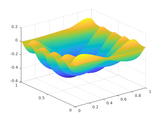
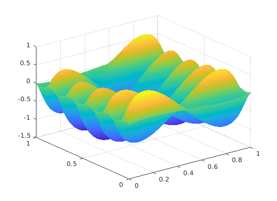
Figure 5: Solutions of the problem (20) in the constant coefficient case. On the left, the problem with $\alpha_{1}=1.7,\alpha_{2}=1.9$. On the right, the one with $\alpha_{1}=1.3,\alpha_{2}=1.7$. The solutions are plotted at the final time step $t=7$.

$N$	$t_{\mathrm{HODLR}}$	$t_{\mathrm{BSS}}$	$\mathrm{rank}_{\epsilon}$	$\text{qsrank}_{\epsilon}$
$512$	$0.63$	$2.53$	$18$	$10$
$1{,}024$	$1.05$	$4.21$	$19$	$10$
$2{,}048$	$1.97$	$7.5$	$20$	$11$
$4{,}096$	$4.19$	$18.34$	$21$	$11$
$8{,}192$	$7.24$	$31.9$	$21$	$11$
$16{,}384$	$17.05$	$55.86$	$21$	$11$
$32{,}768$	$32.48$	$107.85$	$22$	$11$
$65{,}536$	$79.25$	$221.83$	$23$	$11$

Table 5: Timings for the solution of the problem (20) with constant coefficients as in (24) using the HODLR solver and the approach presented in [8]. The exponents are set to $\alpha_{1}=1.7$ and $\alpha_{2}=1.9$.

We note that the HODLR solver outperforms the BSS approach in all our tests, although the advantage is slightly reduced when $N$ increases. For solving Toeplitz linear systems, we have used the preconditioner in [12], which turned out to perform better than the circulant one. However, when considering the the nonconstant coefficients case, a small growth in the number of iterations can be seen as $N$ increases. In particular, the preconditioner based on the first derivative $P_{1}$ seems to be less robust, while $P_{2}$ is less sensitive to changes in the coefficients, the time-step, and other parameters. In this example, it turned out that $P_{2}$ is always the most efficient choice, even when $\alpha_{1}$ is as low as $1.3$, and therefore it is the one employed in the tests of the BSS method.

Note that in the case with $\alpha_{1}=1.3$ the preconditioner $P_{2}$ works well (the number of iterations does not increase with $N$), but the number of iterations is not particularly low (typical figures are in the range of 15 to 20, sometimes more); therefore, this case is particularly favorable to the HODLR approach, which indeed outperforms BSS by a factor of about $6$ in time at the larger tested size, $N=$65536$$. The results are reported in Table 4 and Table 6.

$N$	$t_{\mathrm{HODLR}}$	$t_{\mathrm{BSS}}$	$\mathrm{rank}_{\epsilon}$	$\text{qsrank}_{\epsilon}$
$512$	$0.34$	$3.84$	$14$	$10$
$1{,}024$	$0.61$	$6.43$	$14$	$11$
$2{,}048$	$1.14$	$11.68$	$16$	$12$
$4{,}096$	$2.59$	$30.15$	$16$	$12$
$8{,}192$	$4.86$	$51.19$	$16$	$13$
$16{,}384$	$8.79$	$84.68$	$17$	$13$
$32{,}768$	$19.24$	$153.98$	$15$	$14$
$65{,}536$	$46.13$	$282.35$	$15$	$14$

Table 6: Timings for the solution of the problem (20) with variable coefficients as in (24) using the HODLR solver and the approach presented in [8]. The exponents are set to $\alpha_{1}=1.3$ and $\alpha_{2}=1.7$. The times reported are expressed in seconds.

$N$	$t_{\mathrm{HODLR}}$	$t_{\mathrm{BSS}}$	$\mathrm{rank}_{\epsilon}$	$\text{qsrank}_{\epsilon}$
$512$	$0.6$	$2.68$	$18$	$10$
$1{,}024$	$1.01$	$4.36$	$19$	$10$
$2{,}048$	$2.03$	$7.69$	$21$	$11$
$4{,}096$	$4.06$	$16.85$	$22$	$11$
$8{,}192$	$8.52$	$28.27$	$22$	$11$
$16{,}384$	$17.73$	$48.64$	$22$	$11$
$32{,}768$	$36.82$	$88.81$	$24$	$12$
$65{,}536$	$95.43$	$170.94$	$25$	$12$

Table 7: Timings for the solution of the problem (20) with variable coefficients as in (24) using the HODLR solver and the approach presented in [8]. The exponents are set to $\alpha_{1}=1.7$ and $\alpha_{2}=1.9$.

5.2 A 2D finite element discretization

The example considered in this section is given by problem (20) on the domain $[0,1]^{2}$ in the constant coefficients case and with source term, and solution at time $0$ defined as follows:

$$f(x,y,t)=\begin{cases}1&(x,y)\in H\\ 0&\text{otherwise}\\ \end{cases},\qquad u(x,y,0)=f(x,y,0),\qquad H=\left\{\frac{3}{8}\leqslant x,y\leqslant\frac{5}{8}\right\},$$

similarly to what is done in [13]. The fractional exponents are chosen as $\alpha_{1}=1.3$ and $\alpha_{2}=1.7$. We used the piecewise linear functions described in [13] as basis for the finite element discretization. For simplicity, we consider a uniform grid for the nodes defining the hat functions, which yields a Toeplitz matrix whose symbol is explicitly given in [30]. Therefore, the same strategy used in the previous section can be used to recover a rank structured representation of the matrix, which is guaranteed to exist thanks to Theorem 3.27.

We consider the time step of $\Delta t=0.1$, and the discretization in time is done by the backward Euler method. The truncation thresholds are set exactly as in the previous example. We have performed tests changing the number of grid points used in each direction, and the timings are reported in Table 8.

$N$	$t_{\mathrm{HODLR}}$	$t_{\mathrm{BSS}}$	$\mathrm{rank}_{\epsilon}$	$\text{qsrank}_{\epsilon}$
$512$	$0.22$	$1.45$	$10$	$13$
$1{,}024$	$0.42$	$2.01$	$11$	$14$
$2{,}048$	$0.8$	$5.52$	$12$	$13$
$4{,}096$	$1.8$	$7.91$	$13$	$13$
$8{,}192$	$3.05$	$22.53$	$13$	$14$
$16{,}384$	$7.18$	$42.35$	$14$	$14$
$32{,}768$	$12.88$	$84.94$	$15$	$15$
$65{,}536$	$31.66$	$122.62$	$14$	$15$

Table 8: Timings for the solution of the problem (20) using a finite element discretization. The exponents are set to $\alpha_{1}=1.3$ and $\alpha_{2}=1.7$.

We notice that the timings behave linearly, and the rank of the solution stabilizes around $14$. Since the matrix equation has Toeplitz coefficients, we can directly compare with the approach by Breiten, Simoncini, and Stoll in [8]. A spectral reasoning similar to the one in [12] justifies the use of preconditioner $P_{2}$ for solving Toeplitz linear systems also in the finite elements setting. As for the finite differences, the use of rank structures turns out to be more efficient. However, we stress that our method remains applicable without modifications even if one considers non-uniform grids, in contrast to the BSS approach. The only difference is in the construction of the rank structured representation, which needs to be performed relying on Theorem 3.27.

6 Conclusions and outlook

In this paper we have presented a rigorous theoretical analysis of the rank of the off-diagonal blocks in 1D discretizations of fractional differential operators. We have analyzed different formulations, namely the Grünwald-Letnikov (shifted and non-shifted) finite difference schemes, as well as finite element approaches. In the latter class, we have shown that the stiffness matrix of the finite element discretization is rank structured under mild hypotheses on the finite element basis.

We have then shown that it is possible to obtain parametrizations of such rank structures very efficiently in the HODLR format, and this can be used to solve 1D fractional differential equations (possibly with time dependence), as well as to analyze a broad range of 2D problems where the differential operator is separable, and thus the equation can be recast in matrix form [8]. This includes, but is not limited to, fractional diffusion equations.

In our numerical experiments we have shown that HODLR-based solvers often outperform previous approaches relying on Toeplitz-structured preconditioners. This is particularly advantageous in the 2D setting, where in the projection scheme used to deal with the matrix equation one needs to solve several linear systems, and the computation of the LU factorization in HODLR format can be amortized among more operations.

The machinery extends to 2D equations whose associated matrix equation has a right-hand side in the HODLR format. In this case, it is necessary to replace the extended Krylov method with the divide and conquer technique presented in [28].

Further improvements can be achieved replacing the HODLR format with more sophisticated structures that rely on nested bases for the representation of the off-diagonal blocks, as HSS and $\mathcal{H}^{2}$ matrices [51, 24]. This would remove some log factors from the asymptotic complexity of time and memory consumption, and might be subject of future work.

References

• [1] ITER - the way to new energy. https://www.iter.org/.
• [2] J. Bai and X.-C. Feng. Fractional-order anisotropic diffusion for image denoising. IEEE Trans. Image Process., 16(10):2492–2502, 2007.
• [3] B. Beckermann. An error analysis for rational Galerkin projection applied to the Sylvester equation. SIAM J. Numer. Anal., 49(6):2430–2450, 2011.
• [4] B. Beckermann and A. Townsend. On the singular values of matrices with displacement structure. SIAM J. Matrix Anal. Appl., 38(4):1227–1248, 2017.
• [5] M. Berljafa and S. Güttel. Generalized rational Krylov decompositions with an application to rational approximation. SIAM J. Matrix Anal. Appl., 36(2):894–916, 2015.
• [6] R. Bhatia. Infinitely divisible matrices. Amer. Math. Monthly, 113(3):221–235, 2006.
• [7] S. Börm, L. Grasedyck, and W. Hackbusch. Hierarchical matrices. Lect. notes, 21:2003, 2003.
• [8] T. Breiten, V. Simoncini, and M. Stoll. Low-rank solvers for fractional differential equations. Electron. Trans. Numer. Anal., 45:107–132, 2016.
• [9] L. A. Caffarelli and P. R. Stinga. Fractional elliptic equations, Caccioppoli estimates and regularity. Ann. Inst. H. Poincaré Anal. Non Linéaire, 33(3):767–807, 2016.
• [10] D. del Castillo-Negrete, B. Carreras, and V. Lynch. Fractional diffusion in plasma turbulence. Phys. Plasmas, 11(8):3854–3864, 2004.
• [11] W. Deng, B. Li, W. Tian, and P. Zhang. Boundary problems for the fractional and tempered fractional operators. Multiscale Model. Simul., 16(1):125–149, 2018.
• [12] M. Donatelli, M. Mazza, and S. Serra-Capizzano. Spectral analysis and structure preserving preconditioners for fractional diffusion equations. J. Comput. Phys., 307:262–279, 2016.
• [13] B. Duan, Z. Zheng, and W. Cao. Finite element method for a kind of two-dimensional space-fractional diffusion equation with its implementation. American Journal of Computational Mathematics, 5(02):135, 2015.
• [14] Y. Eidelman, I. Gohberg, and I. Haimovici. Separable type representations of matrices and fast algorithms. Vol. 1, volume 234 of Operator Theory: Advances and Applications. Birkhäuser/Springer, Basel, 2014.
• [15] V. J. Ervin and J. P. Roop. Variational formulation for the stationary fractional advection dispersion equation. Numer. Methods Partial Differential Equations, 22(3):558–576, 2006.
• [16] D. Fasino. Spectral properties of Toeplitz-plus-Hankel matrices. Calcolo, 33(1-2):87–98 (1998), 1996. Toeplitz matrices: structures, algorithms and applications (Cortona, 1996).
• [17] M. Fiedler. Notes on Hilbert and Cauchy matrices. Linear Algebra Appl., 432(1):351–356, 2010.
• [18] C. Garoni and S. Serra-Capizzano. Generalized locally Toeplitz sequences: theory and applications. Vol. I. Springer, Cham, 2017.
• [19] G. H. Golub, F. T. Luk, and M. L. Overton. A block Lánczos method for computing the singular values of corresponding singular vectors of a matrix. ACM Trans. Math. Software, 7(2):149–169, 1981.
• [20] L. Grasedyck. Singular value bounds for the cauchy matrix and solutions to sylvester equations. Technical report, Technical report 13, Germany: University Kiel, 2001.
• [21] L. Grasedyck, W. Hackbusch, and S. Le Borne. Adaptive geometrically balanced clustering of $\mathscr{H}$-matrices. Computing, 73(1):1–23, 2004.
• [22] M. H. Gutknecht. Block krylov space methods for linear systems with multiple right-hand sides. In The Joint Workshop on Computational Chemistry and Numerical Analysis (CCNA2005), 2005.
• [23] W. Hackbusch. A sparse matrix arithmetic based on H-matrices. Part I: Introduction to H-matrices. Computing, 62(2):89–108, 1999.
• [24] W. Hackbusch. Hierarchical matrices: algorithms and analysis, volume 49. Springer, 2015.
• [25] M. Heyouni. Extended Arnoldi methods for large low-rank Sylvester matrix equations. Appl. Numer. Math., 60(11):1171–1182, 2010.
• [26] X.-Q. Jin, F.-R. Lin, and Z. Zhao. Preconditioned iterative methods for two-dimensional space-fractional diffusion equations. Commun. Comput. Phys., 18(2):469–488, 2015.
• [27] L. Knizhnerman and V. Simoncini. Convergence analysis of the extended Krylov subspace method for the Lyapunov equation. Numer. Math., 118(3):567–586, 2011.
• [28] D. Kressner, S. Massei, and L. Robol. Low-rank updates and a divide-and-conquer method for linear matrix equations. SIAM J. Sci. Comput., 41(2):A848–A876, 2019.
• [29] S.-L. Lei and H.-W. Sun. A circulant preconditioner for fractional diffusion equations. J. Comput. Phys., 242:715–725, 2013.
• [30] Z. Lin and D. Wang. A finite element formulation preserving symmetric and banded diffusion stiffness matrix characteristics for fractional differential equations. Comput. Mech., pages 1–27, 2017.
• [31] Y. Liu, Y. Yan, and M. Khan. Discontinuous Galerkin time stepping method for solving linear space fractional partial differential equations. Appl. Numer. Math., 115:200–213, 2017.
• [32] S. Massei, D. Palitta, and L. Robol. Solving rank-structured Sylvester and Lyapunov equations. SIAM J. Matrix Anal. Appl., 39(4):1564–1590, 2018.
• [33] S. Massei and L. Robol. Hierarchical matrix toolbox. GitHub repository: https://github.com/numpi/hm-toolbox, 2015.
• [34] M. M. Meerschaert and C. Tadjeran. Finite difference approximations for fractional advection-dispersion flow equations. J. Comput. Appl. Math., 172(1):65–77, 2004.
• [35] H. Moghaderi, M. Dehghan, M. Donatelli, and M. Mazza. Spectral analysis and multigrid preconditioners for two-dimensional space-fractional diffusion equations. J. Comput. Phys., 350:992–1011, 2017.
• [36] J. Pan, M. Ng, and H. Wang. Fast preconditioned iterative methods for finite volume discretization of steady-state space-fractional diffusion equations. Numer. Algorithms, 74(1):153–173, 2017.
• [37] J. Pan, M. K. Ng, and H. Wang. Fast iterative solvers for linear systems arising from time-dependent space-fractional diffusion equations. SIAM J. Sci. Comput., 38(5):A2806–A2826, 2016.
• [38] H.-K. Pang and H.-W. Sun. Multigrid method for fractional diffusion equations. J. Comput. Phys., 231(2):693–703, 2012.
• [39] I. Podlubny. Fractional differential equations: an introduction to fractional derivatives, fractional differential equations, to methods of their solution and some of their applications, volume 198. Academic press, 1998.
• [40] M. Raberto, E. Scalas, and F. Mainardi. Waiting-times and returns in high-frequency financial data: an empirical study. Physica A, 314(1):749–755, 2002.
• [41] J. P. Roop. Computational aspects of FEM approximation of fractional advection dispersion equations on bounded domains in ${\mathbb{R}}^{2}$. J. Comput. Appl. Math., 193(1):243–268, 2006.
• [42] H. D. Simon and H. Zha. Low-rank matrix approximation using the Lanczos bidiagonalization process with applications. SIAM J. Sci. Comput., 21(6):2257–2274, 2000.
• [43] V. Simoncini. A new iterative method for solving large-scale Lyapunov matrix equations. SIAM J. Sci. Comput., 29(3):1268–1288, 2007.
• [44] V. Simoncini. Computational methods for linear matrix equations. SIAM Review, 58(3):377–441, 2016.
• [45] W. Tian, H. Zhou, and W. Deng. A class of second order difference approximations for solving space fractional diffusion equations. Math. Comp., 84(294):1703–1727, 2015.
• [46] A. Townsend. Computing with functions in two dimensions. PhD thesis, University of Oxford, 2014.
• [47] A. Townsend and L. N. Trefethen. An extension of Chebfun to two dimensions. SIAM J. Sci. Comput., 35(6):C495–C518, 2013.
• [48] R. Vandebril, M. Van Barel, and N. Mastronardi. Matrix computations and semiseparable matrices. Linear systems, volume 1. Johns Hopkins University Press, Baltimore, MD, 2008.
• [49] H. Wang, K. Wang, and T. Sircar. A direct $O(N\log^{2}N)$ finite difference method for fractional diffusion equations. J. Comput. Phys., 229(21):8095–8104, 2010.
• [50] R. Wang, Y. Li, M. W. Mahoney, and E. Darve. Structured block basis factorization for scalable kernel matrix evaluation. arXiv preprint arXiv:1505.00398, 2015.
• [51] J. Xia, S. Chandrasekaran, M. Gu, and X. S. Li. Fast algorithms for hierarchically semiseparable matrices. Numer. Linear Algebra Appl., 17(6):953–976, 2010.
• [52] X. Zhao, X. Hu, W. Cai, and G. E. Karniadakis. Adaptive finite element method for fractional differential equations using hierarchical matrices. Comput. Methods Appl. Mech. Engrg., 325:56–76, 2017.