Quantifying the impact of phonon scattering on electrical and thermal transport in quantum dots

Abstract

We report the inclusion of phonon scattering to our recently established numerical package QmeQ for transport in quantum dot systems. This enables straightforward calculations for a large variety of devices. As examples we show (i) transport in a double-dot structure, where energy relaxation is crucial to match the energy difference between the levels, and (ii) the generation of electrical power by contacting cold electric contacts with quantum dot states, which are subjected to heated phonons.

1 Introduction

During the last decades, there has been a large amount of research on the electronic properties and electron transport in nanostructure devices DevoretNature1992 ; TaruchaPRL1996 ; KouwenhovenScience1997 ; ReimannRMP2002 . A tremendous progress has been made in this area and new exciting optical, electronic, and thermoelectric applications have been suggested ThelanderMaterialsToday2006 ; BoukaiNature2008 ; AgarwalApplPhysA2006 ; KoskiPNAS2014 ; KarimiNL2018 .

The confinement of electrons in nanostructure devices leads to discrete electronic states and hence to quantized electron transport KastnerRMP1992 ; AverinPRB1991 ; FultonPRL1987 ; AshooriNature1996 ; KouwenhovenZPhysBCondMat1991 . Therefore the transport properties become influenced by this quantization that can be seen as Coulomb blockade AverinJLTP1986 ; AverinPRB1991 ; DevoretNature1992 and resonant tunneling GurvitzPRB1996 . Likewise the electrons, phonons can also be confined in nanostructure devices. The confinement of phonons leads to different modes with a one-dimensional dispersion StroscioJAP1994 . An example of such effects is the temperature dependence of resistivity in Si nanowires VauretteAPL2008 . Another example is probing of the individual phonon modes in transport WeberPRL2010 . This new kind of phonon spectroscopy allows to get information on the energetic location of the phonon modes as well as electron phonon interaction strength.

To understand the role of different interactions in the many-body physics of nanostructures, some studies have focused on the details of electron-electron KuoPRB2010 ; AzemaPhysRevB2014 , electron-phonon LeijnsePRB2010 , and electron-photon HenrietPhysRevB2015 coupling effects on nonlinear thermoelectric transport. Moreover, a lot of progress has been made both in formulating the many-body theories and developing experimental methods in this subject. The recent technological progress in the design and fabrication of semiconductor nanostructures can help to achieve a better understanding of how the electron-phonon coupling affects the transport in nanostructures.

There is a large variety of theoretical approaches to calculate transport through nanostructure systems.BruusBook2004 ; TimmPRB2008 ; RyndykBook2009 ; SchallerBook2014 For systems, where Coulomb interaction is dominant, single particle transmission approaches are insufficient and different types of master equations have been established. Recently, some of us published a software package called QmeQ (Quantum master equation for Quantum dot transport calculations) KirsanskasComputPhysCommun2017 , which allows a simple comparison of several Master equations for quantum dot systems with full Coulomb interaction. Here we show the first results of phonon scattering integration into this package.

As a model system, we consider a spinful double dot with tunable energy levels and compare with experimental data from WeberPRL2010 . Double quantum dots are well-known to be suitable systems to study essential concepts of quantum mechanics, due to their high tunability. Furthermore, we consider non-equilibrium phonon distributions, which can establish particle current flow against the bias SothmannNJP2013 .

2 QmeQ and its extension for phonon interaction

The package QmeQ KirsanskasComputPhysCommun2017 is designed to study transport in quantum dot systems described by the general Hamiltonian,

$$H_{\textrm{sys}}=\underset{n\sigma}{{\displaystyle\sum}}E_{n}d^{{\dagger}}_{n\sigma}d^{\phantom{{\dagger}}}_{n\sigma}+\underset{nm\sigma}{{\displaystyle\sum}}\Omega_{nm}d^{{\dagger}}_{n\sigma}d^{\phantom{{\dagger}}}_{m\sigma}+\frac{1}{2}\underset{mnkl}{{\displaystyle\sum}}\underset{\sigma\sigma^{\prime}}{{\displaystyle\sum}}V_{mnkl}d^{{\dagger}}_{m\sigma^{\phantom{\prime}}}d^{{\dagger}}_{n\sigma^{\prime}}d^{\phantom{{\dagger}}}_{k\sigma^{\prime}}d^{\phantom{{\dagger}}}_{l\sigma},$$ (1)

where $d^{{\dagger}}_{n\sigma}$ is the electron creation operator in the system for a level with energy $E_{n}$ and spin $\sigma$. $\Omega_{nm}$ describes the coupling between the single-particle levels $m$ and $n$, and the last part quantifies the electron-electron interaction with different Coulomb matrix elements $V_{mnkl}$. Using a Fock basis, $H_{\textrm{sys}}$ is diagonalized providing the many-particle eigenstates of the form

$$\left|a\right\rangle=\underset{n}{\sum}b_{n}d^{{\dagger}}_{n_{1}}d^{{\dagger}}_{n_{2}}...d^{{\dagger}}_{n_{Na}}\left|0\right\rangle,$$ (2)

where $n_{i}$ represents the $i$th single particle state in the Slater determinant determined by the index $n=(n_{1},n_{2,},...,n_{Na})$ with $N_{a}$ number of particles.

The tunneling and the lead Hamiltonians are

$$H_{\textrm{Leads}}=\underset{k\sigma l}{{\displaystyle\sum}}E_{k\sigma\ell}c^{{\dagger}}_{k\sigma l}c^{\phantom{{\dagger}}}_{k\sigma\ell},\quad H_{T}=\underset{n,k\sigma\ell}{{\displaystyle\sum}}(t_{n\ell}d^{{\dagger}}_{n\sigma}c^{\phantom{{\dagger}}}_{k\sigma\ell}+\mathrm{H.c.}),$$ (3)

where $c^{{\dagger}}_{k\sigma\ell}$ denotes the electron creation operators in the leads with index $\ell$ (typically R,L for right and left lead, respectively) and $k$ labels the spatial wave-functions of the continuum of states. We assume a thermal distribution with electrochemical potential $\mu_{\ell}$ and temperature $T_{\ell}$ for each lead. A bias $V$ applied to the leads provides $\mu_{L/R}=\pm eV/2$, where $e$ is the elementary charge. The tunneling Hamiltonian, $H_{T}$, can be expressed by the many-particle eigenstates

$$H_{T}=\underset{ab,k\ell\sigma}{\sum}(T_{{}_{ba}}(\ell\sigma)\left|b\right\rangle\left\langle a\right|c^{\phantom{{\dagger}}}_{k\ell\sigma}+\mathrm{H.c.})\quad\textrm{with}\quad T_{{}_{ba}}(\ell\sigma)=\underset{n}{\sum}t_{n\ell}\left\langle b\right|d^{{\dagger}}_{n\sigma}\left|a\right\rangle.$$ (4)

Here we use the letter convention restricting the combination of states $|a\rangle,|a\prime\rangle,|b\rangle$ to $N_{b}=N_{a}+1$, and $N_{a}=N_{a\prime}$.

QmeQ is able to calculate the current for a stationary state with different approaches: the Pauli (classical) master equation BreuerBook2006 ; BruusBook2004 , first-order Redfield WangsnessPR1953 ; RedfieldIBM1957 and first/second-order von Neumann approaches PedersenPRB2005a ; PedersenPHE2010 , and a master equation in a Lindblad form LindbladCMP1976 using the Position and Energy Resolved Lindblad Approach (PERLind) of Ref. KirsanskasPRB2018 .

In this study we calculate the impact of electron-phonon interaction on the particle current through the device with different first-order approaches. The phonons are modeled as simple non-interacting Bosonic modes

$$H_{ph}=\underset{q}{\sum}\hbar\omega_{q}b^{{\dagger}}_{q}b^{\phantom{{\dagger}}}_{q},$$ (5)

were $b^{{\dagger}}_{q}$ creates a phonon in a mode $q$. The electron-phonon interaction is given by

$$H_{e-ph}=\underset{nm\sigma,q}{\sum}g_{nm}^{q}d^{{\dagger}}_{n\sigma}d^{\phantom{{\dagger}}}_{m\sigma}(b^{{\dagger}}_{\overline{q}}+b^{\phantom{{\dagger}}}_{q}).$$ (6)

with the matrix elements $g_{nm}^{q}$ and $\overline{q}$ denoting the complex conjugate state of $q$. Since the phonon coupling to the free electrons in the leads is very small compared to the electron phonon coupling in the central region, see Ref. WingreenPRB1989 , only the electron phonon coupling in the dot will be considered. Within the lowest nonvanishing order in the phonon coupling studied here, coherent superpositions of states with different phonon number are neglected.

We consider deformation potential coupling to the phonons, which is given by the divergence of the displacement following LindwallPRL2007 . The corresponding coupling matrix element for the first acoustic phonon mode coupled to the electrons via the deformation potential can be expressed by

$$g_{nm}^{q1}=\int d^{3}r\,\varPsi_{n}^{\ast}(\mathbf{r})D\nabla\cdot\mathbf{u}_{q1}(\mathbf{r})\varPsi_{m}(\mathbf{r}).$$ (7)

Here $\mathbf{u}_{q1}(\mathbf{r})$ is the displacement and $D$ is the deformation potential coefficient. We express the electron-phonon coupling matrix element, $g_{nm}^{q}=g(q)y_{nm}^{q}$, in terms of a state-independent overall strength $g(q)$ and a dimensionless coefficient

$$y_{nm}^{q}=\int d^{3}r\,\varPsi_{n}^{\ast}(\mathbf{r})\textrm{e}^{\textrm{i}\mathbf{q}\cdot\mathbf{r}}(\mathbf{r})\varPsi_{n^{\prime}}(\mathbf{r}).$$ (8)

By assuming that $y_{nm}^{q}$ is $q$-independent (e.g. by choosing a characteristic value), we obtain

$$y_{nm}^{q}\approx y_{nm},\quad y_{nm}^{\overline{q}}\approx\overline{y}_{nm}=y_{mn}^{*},$$ (9)

and we can collect all the energy dependence in the spectral density

$$J(E)=\underset{q}{\sum}\left|g(q)\right|^{2}\delta(E-\hbar\omega_{q}).$$ (10)

Both $J(E)$ and $y_{nm}$ are required inputs in the new version of QmeQ with the possibility to add further vibrational modes as independent processes in an analogous way.

3 Results

In order to illustrate the performance of QmeQ, we simulate the nanowire double-dot system studied in Ref. WeberPRL2010 , and compare the results with experimental data. Each dot has a ground level $E_{L/R}$ and an excited level $E_{L/R}+5.5$ meV (both spin degenerate), where $E_{L}$ and $E_{R}$ can be individually shifted by plunger gates. The two dots are coupled to each other and to the leads by tunnel barriers. We use the InAs nanowire material parameters (see Ref. WeberPRL2010 ) to calculate the spectral density for the lowest, one-dimensional phonon mode:

$$J(E)=3.8804\times 10^{-4}E.$$ (11)

The matrix elements $y_{nm}$ for the relevant single-particle levels $m$ and $n$ are calculated from Eq. (8), where the corresponding electron wave functions are assumed to be $\varPsi_{1}(\mathbf{r})=a^{-{3}/{2}}\pi^{-{3}/{4}}e^{-{(x^{2}+y^{2}+z^{2})}/{2a^{2}}}$ for the ground state and $\varPsi_{3}(\mathbf{r})=\sqrt{2}za^{-{5}/{2}}\pi^{-{3}/{4}}e^{-{(x^{2}+y^{2}+z^{2})}/{2a^{2}}}$ for the excited state of the left dot with the Gaussian radius $a=5.8$ nm LindwallPRL2007 . The corresponding states for the right dot ($n=2,4$) are shifted by $d=120$ m, in $z$-direction. For $qa\ll 1$, $q$ only enters as the phase $e^{iqd}$ for matrix elements with different dots, and we use a typical value $e^{iqd}=e^{i\pi/3}$ to remove the $q$-dependence.

The electron-electron Coulomb matrix elements are calculated with the same methods as described in GoldozianSciRep2016 . We consider intradot interactions, $U=12$ meV, as the interaction between electrons in the same dot and inter-dot interaction, $U_{n}=2.5$ meV, as the interaction between electrons in the neighboring dots. The couplings between the energy levels in the dots and the left and right leads are ${\Gamma_{L}}$ = 90 neV and ${\Gamma_{R}}$ = 10 neV, respectively WeberPRL2010 .

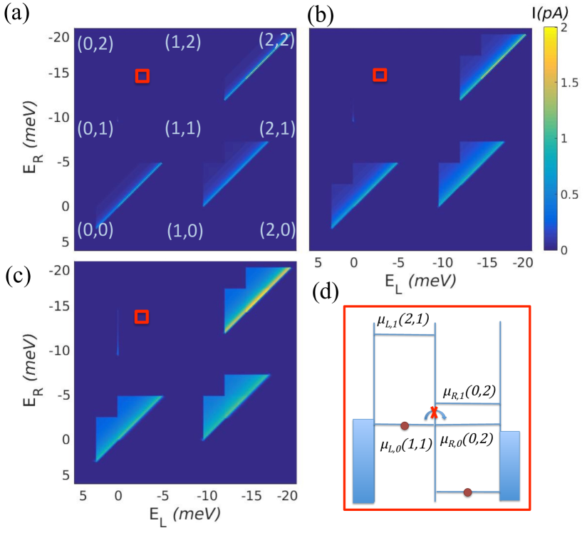
Figure 1: Stability diagrams of the double dot system ranging from weak to strong inter-dot tunnel coupling, i.e., (a) $\Omega$ = 0.005 meV, (b) $\Omega$ = 0.01 meV (c) $\Omega$ = 0.02 meV. The bias is $V=5$ mV for all of them. The diagram in (d) shows schematically the removal energies $\mu_{i,n}(N_{l},N_{r})$ at the operation point denoted by red squares in (a), (b), and (c). At this point the current is suppressed due to Pauli spin blockade. [$\mu_{i,n}(N_{l},N_{r})$ is the energy of an electron removed from the level $n$ ($0=$ ground, $1=$ excited) of dot $i$ (left or right) where $N_{l/r}$ is the number of electrons in the left/right dot.]

Fig. 1 shows the current as a function of the left and the right dot energy levels ($E_{L}$ and $E_{R}$) for three different tunnel coupling strengths $\Omega$. We can see the lowest inter-dot transitions between different level configurations of the double dot, which give rise to the current. What stands out in this figure is the current increase in the presence of phonon scattering close to the current peaks from the resonance. This is a result of the electron-phonon scattering which is an inelastic process. The triangles of finite current appear due to the phonon emission process. When the energy level in the left dot is higher than the one in the right dot, electrons in the left dot are able to transport through the right dot by emitting phonons. The absorption of phonons does not play any role since $k_{B}T\ll eV$. We observed a pair of overlapping full bias triangles, for each transition, due to the inter-dot Coulomb interactions. These triangles are more pronounced in the plots corresponding to stronger tunnel coupling between the dots (Fig. 1(b) and Fig. 1(c)).

On the left top of the plots current suppression due to Pauli spin blockade OnoScience2002 ; JohnsonPRB2005 can be seen. This corresponds to the transition $(1,1)\longrightarrow(0,2)$, where current is blocked, if both dots are occupied by the same spin. Fig. 1(d) shows the energy levels at this operation point.

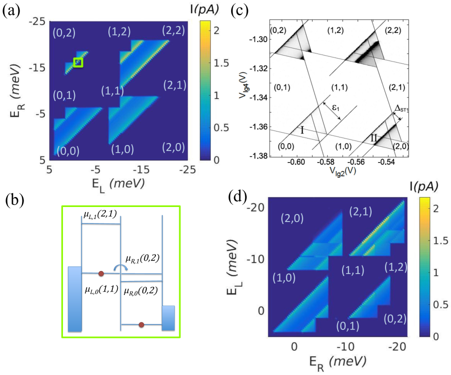
Figure 2: (a) Stability diagram of the double dot system with the inter-dot tunnel coupling $\Omega$ = $0.02$ meV and an increased bias $V=8$ mV compared to Fig. 1. Here the combination of electron-phonon coupling and high bias lifts the Pauli spin blockade as sketched in panel (b). (c) Experimental data (with different bias polarity) taken from the supplementary material of WeberPRL2010 . The highest current is $\approx 1$ pA. (d) Stability diagram for the same parameters as panel (a) including the exchange interaction, $U_{ex}=3$ meV, displayed with swapped axes to reflect the different bias polarity in (c).

Figure 2(a) depicts the results for the same system as Fig. 1, but with higher bias. As we can see here, in contrast to Fig. 1, the transition $(1,1)\longrightarrow(0,2)$ is possible, since the high bias creates a new transport channel via the excited state. As the schematic diagram in Fig. 2(b) explains, electrons form the excitation $\mu_{L,0}(1,1)$ can now be in resonance with $\mu_{R,1}(0,2)$, while the lower lying two-particle state $\mu_{R,0}(0,2)$ is still emptied to the right lead. The triangular regions as well as the truncated triangle between the (1,1) and (0,2) region fully agree with experimental data displayed in Fig. 2(c). Note that the bias polarity was chosen differently in the experiment, so that (0,2) compares to (2,0) in our definition. While the line due to tunneling via the excited state is shifted from the ground state by a fixed amount 5.5 meV for all triangles in our simulation, see Fig. 2(a), two different separations can be seen in the experiment, depending on the charging of the receiving quantum dot. This difference can be attributed to the exchange interaction within the dots. Assuming $U_{ex}=3$ meV, Fig. 2(d) provides a better agreement with the experiment. We observe, that Fig. 2(d) contains some additional features in the triangles with two electrons in the left dot, if a spin triplet becomes possible. These are not observed in the experiment, most likely due to spin relaxations on nanosecond (or shorter) time scales. Such spin-relaxation also explains the incomplete spin blockade observed in the experiment.

As a second example we consider the impact of a heated phonon distribution in the double dot system, which can act as a heat engine SothmannNJP2013 ; JiangPhysRevApplied2017 . A similar scenario can also arise due to a noise sourceEntinPRB2017 . Here we consider the same system as before, but neglect the excited levels. The setup is sketched in the right panel of Fig. 3. While keeping the electron leads at $T_{C}=60$ mK, we apply a different temperature $T_{H}$ in the phonon distribution. Fig. 3 shows the current as a function of the difference between the energy levels of the dots, $\Delta=E_{L}$ - $E_{R}$, which are shifted symmetrically with respect to the electrochemical potential in the leads at zero bias. We find, that an asymmetry in the level energies drives a current through the quantum dot system, where (for $T_{H}>T_{C}$) the net particle current goes from the lower to the higher level. The reason is that the thermal distributions in the contacts result in a significant difference between the occupations of the upper and lower dot level. For the larger phonon temperature, this implies a dominance of phonon absorption over phonon emission between these levels, actually driving the current by taking heat from the phonon system. As thoroughly discussed in Refs. SothmannNJP2013 ; JiangPhysRevApplied2017 this acts as a heat engine, if this current flows against an electric bias. This can be seen in the inset: For a positive detuning $\Delta\approx 0.08$ meV, i.e., $E_{L}>E_{R}$, the current flows against the bias polarity. In contrast to the treatment of Ref. JiangPhysRevApplied2017 the use of QmeQ allows for a straightforward implementation of the full many-body interaction in the transport calculations.

These calculations were performed with the Pauli master equation, while the Redfield and first order von Neumann (1vN) approaches gave the same results for these parameters, where ${\Gamma}$ is much smaller than the level splitting and non-diagonal elements of the density matrix are not relevant KirsanskasComputPhysCommun2017 ; GoldozianSciRep2016 . However, in the case where $\Omega$ is less than ${\Gamma}$, as it is shown in Fig. 4, coherences become important and the Pauli master equation is not reliable. Fig. 4(a) shows the current as a function of $\Delta$, for Pauli, Redfield, and 1vN approaches. As it can be seen the current is reduced in the Redfield and 1vN approaches where the coherences are important. Fig. 4(b) displays the zero bias current as a function of $\Delta$ for $T_{C}$ = $T_{H}$ = 60 mK. Here no current should flow which is recovered by the Pauli master equation. However, the Redfield and 1vN approaches show a very small current as they do not fully satisfy thermal detailed balance. These violations are actually three orders of magnitude smaller than the features studied in Fig. 4(a) and thus do not affect the main results.

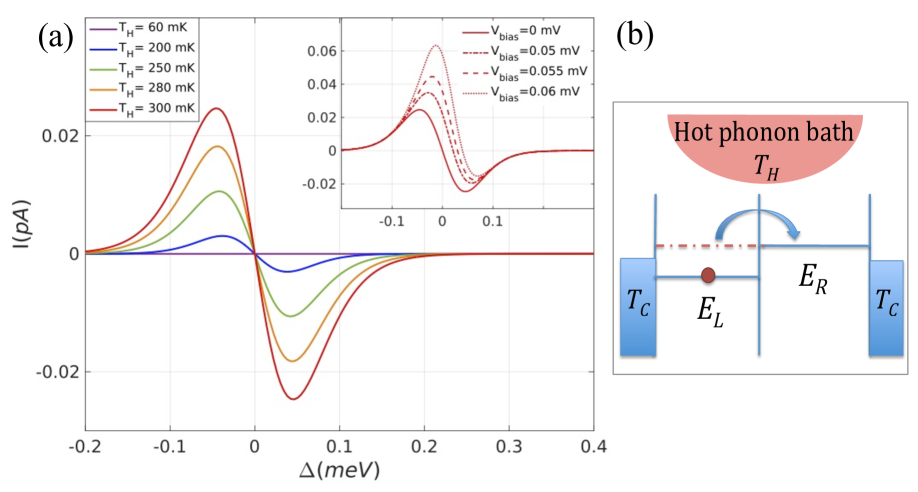
Figure 3: (a) Zero-bias current as a function of $\Delta$, the difference between the energy levels of the dots, for different phonon temperatures. Inset: current as a function of $\Delta$ for different biases and $T_{H}=300$ mK. Further parameter: $T_{C}$ = 60 mK, $\Omega$ = 0.05 meV, ${\Gamma_{L}}$ = ${\Gamma_{R}}$ = 90 neV. (b) A sketch of a double dot system coupled to non-equilibrium phonon bath.

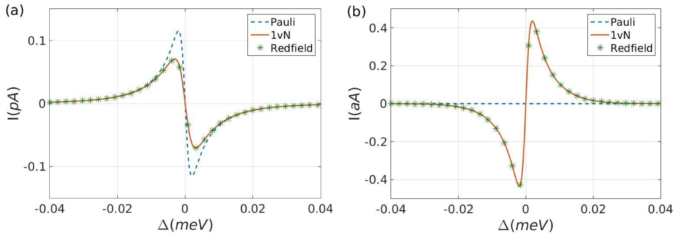
Figure 4: (a) Zero-bias current as a function of $\Delta$, the difference between the energy levels of the dots, for Pauli, Redfield and 1vN approaches. $T_{C}$ = 60 mK, $T_{H}$ = 300 mK, $\Omega$ = 0.001 meV, ${\Gamma_{L}}$ = ${\Gamma_{R}}$ = 0.005 meV. (b) Zero-bias current as a function of $\Delta$, $T_{C}$ = $T_{H}$ = 60 mK, other parameters are the same as (a).

4 Conclusion

We included phonon scattering in QmeQ, which improves the applicability of this versatile simulation package. The new implementation was tested for a double-dot structure, where we could reproduce experimental results and demonstrated the applicability for thermoelectric elements.
Acknowledgments: We thank NanoLund and the Swedish Research Council (Grant No. 621-2012-4024) for financial support.
Author Contributions: BG performed the calculations, produced the figures, and wrote the first draft. GK established the computer program using input from an earlier code by FAD. AW directed the work. All authors contributed to the writing of the manuscript.

References

- (1) M. H. Devoret, D. Esteve, and C. Urbina, Nature 360, 547 (1992).
- (2) S. Tarucha, D. G. Austing, T. Honda, R. J. van der Hage, and L. P. Kouwenhoven, Phys. Rev. Lett. 77, 3613 (1996).
- (3) L. P. Kouwenhoven et al., Science 278, 1788 (1997).
- (4) S. M. Reimann and M. Manninen, Rev. Mod. Phys. 74, 1283 (2002).
- (5) C. Thelander et al., Materials Today 9, 28 (2006).
- (6) A. I. Boukai et al., Nature 451, 168 (2008).
- (7) R. Agarwal and C. Lieber, Applied Physics A 85, 209 (2006).
- (8) J. V. Koski, V. F. Maisi, J. P. Pekola, and D. V. Averin, PNAS 111, 13786 (2014).
- (9) M. Karimi et al., Nano Letters 18, 365 (2018).
- (10) M. A. Kastner, Rev. Mod. Phys. 64, 849 (1992).
- (11) D. V. Averin, A. N. Korotkov, and K. K. Likharev, Phys. Rev. B 44, 6199 (1991).
- (12) T. A. Fulton and G. J. Dolan, Phys. Rev. Lett. 59, 109 (1987).
- (13) R. C. Ashoori, Nature 379, 413 (1996).
- (14) L. P. Kouwenhoven et al., Z. Phys. B - Con. Mat. 85, 367 (1991).
- (15) D. V. Averin and K. K. Likharev, J. Low. Temp. Phys. 62, 345 (1986).
- (16) S. A. Gurvitz and Y. S. Prager, Phys. Rev. B 53, 15932 (1996).
- (17) M. A. Stroscio, K. W. Kim, S. Yu, and A. Ballato, J. Appl. Phys. 76, 4670 (1994).
- (18) F. Vaurette et al., Appl. Phys. Lett. 92, 242109 (2008).
- (19) C. Weber et al., Phys. Rev. Lett. 104, 036801 (2010).
- (20) D. M.-T. Kuo and Y.-C. Chang, Phys. Rev. B 81, 205321 (2010).
- (21) J. Azema, P. Lombardo, and A.-M. Daré, Phys. Rev. B 90, 205437 (2014).
- (22) M. Leijnse, M. R. Wegewijs, and K. Flensberg, Phys. Rev. B 82, 045412 (2010).
- (23) L. Henriet, A. N. Jordan, and K. Le Hur, Phys. Rev. B 92, 125306 (2015).
- (24) H. Bruus and K. Flensberg, Many-Body Quantum Theory in Condensed Matter Physics, Oxford University Press, New York, 2004.
- (25) C. Timm, Phys. Rev. B 77, 195416 (2008).
- (26) D. A. Ryndyk, R. Gutiérrez, B. Song, and G. Cuniberti, Green function techniques in the treatment of quantum transport at the molecular scale, in Energy Transfer Dynamics in Biomaterial Systems, edited by I. Burghardt, V. May, D. A. Micha, and E. R. Bittner, volume 93, pages 213–335, Springer-Verlag, Berlin, Heidelberg, 2009.
- (27) G. Schaller, Open Quantum Systems far from Equilibrium, Springer, Heidelberg, 2014.
- (28) G. Kiršanskas, J. N. Pedersen, O. Karlström, M. Leijnse, and A. Wacker, Comput. Phys. Commun. 221, 317 (2017).
- (29) B. Sothmann, R. Sanchez, A. N. Jordan, and M. Büttiker, New J. Phys. 15, 095021 (2013).
- (30) H.-P. Breuer and F. Petruccione, Open Quantum Systems, Oxford University Press, Oxford, 2006.
- (31) R. K. Wangsness and F. Bloch, Phys. Rev. 89, 728 (1953).
- (32) A. G. Redfield, IBM J. Res. Dev. 1, 19 (1957).
- (33) J. N. Pedersen and A. Wacker, Phys. Rev. B 72, 195330 (2005).
- (34) J. N. Pedersen and A. Wacker, Physica E 42, 595 (2010).
- (35) G. Lindblad, Commun. Math. Phys. 48, 119 (1976).
- (36) G. Kiršanskas, M. Franckié, and A. Wacker, Phys. Rev. B 97, 035432 (2018).
- (37) N. S. Wingreen, K. W. Jacobsen, and J. W. Wilkins, Phys. Rev. B 40, 11834 (1989).
- (38) G. Lindwall, A. Wacker, C. Weber, and A. Knorr, Phys. Rev. Lett. 99, 087401 (2007).
- (39) B. Goldozian, F. A. Damtie, G. Kiršanskas, and A. Wacker, Sci. Rep. 6, 22761 (2016).
- (40) K. Ono, D. G. Austing, Y. Tokura, and S. Tarucha, Science 297, 1313 (2002).
- (41) A. C. Johnson, J. R. Petta, C. M. Marcus, M. P. Hanson, and A. C. Gossard, Phys. Rev. B 72, 165308 (2005).
- (42) J.-H. Jiang and Y. Imry, Phys. Rev. Applied 7, 064001 (2017).
- (43) O. Entin-Wohlman, D. Chowdhury, A. Aharony, and S. Dattagupta, Phys. Rev. B 96, 195435 (2017).