Persistence of normally hyperbolic invariant manifolds in the absence of rate conditions

Abstract

We consider perturbations of normally hyperbolic invariant manifolds, under which they can lose their hyperbolic properties. We show that if the perturbed map which drives the dynamical system preserves the properties of topological expansion and contraction, then the manifold is perturbed to an invariant set. The main feature is that our results do not require the rate conditions to hold after the perturbation. In this case the manifold can be perturbed to an invariant set, which is not a topological manifold. We work in the setting of nonorientable Banach vector bundles, without needing to assume invertibility of the map.

1 Introduction

We will be investigating the persistence under perturbations of invariant sets that are associated with normally hyperbolic invariant manifolds (NHIMs). These perturbations will be such that the manifolds lose their hyperbolic properties.

To be more precise, a manifold $\Lambda$ is said to be a NHIM if it is invariant for a dynamical system and there is a splitting of the state space into three invariant subbundles. One is the tangent bundle to $\Lambda$, the second is the unstable bundle and the third is the stable bundle. The dynamics on the stable bundle is contracting and on the unstable bundle – expanding. The key feature for $\Lambda$ to be normally hyperbolic is that the dynamics on the bundle tangent to $\Lambda$ is weaker than the dynamics on the stable and the unstable bundles. The property of the dominance of the dynamics on the stable/unstable bundles over the tangent bundle is formulated in terms the rate conditions, introduced by Fenichel [Fenichel1, Fenichel4, Fenichel3, Fenichel2], Hirsch, Pugh, Shub [HPS], and later developed by Chaperon [Chap1, Chap2, Chap3].

The main property of NHIMs is that they persist under perturbations. As long as the rate conditions hold, the manifold is present. There are examples though [GonDroJun2014, GonJun2015, Jarnik, TerTodKom2015] for which, in the absence of rate conditions, an invariant manifold can be destroyed to a set which is not even a topological manifold. However, this does not mean that the manifold vanishes or that it is completely destroyed.

This problem has been studied by Floer in [Floer2, Floer]. He introduced a method, which allowed him to establish continuation of NHIMs to invariant sets which preserve the cohomology ring of the manifold under perturbation. We take a different approach, which is based on a good topological alignment expressed by homotopy conditions. We establish existence of an invariant set whose projection onto the base manifold $\Lambda$ is equal to the whole $\Lambda$. The advantage of our method is that it does not rely on the prior existence of a normally hyperbolic invariant manifold and neither does it use perturbation theory. Moreover, we prove a continuation theorem for invariant sets of continuous one-parameter families of maps under the assumption of correct topological alignment. To be more precise, we show that if we extend the system to include the parameter, then, in such an extended phase space, there exists a compact connected component consisting of points belonging to the invariant sets of maps corresponding to varying parameter values.

Our result does not contradict the work of Mañé [Mane]. He shows that if a manifold is persistent, then it has to be normally hyperbolic. What we establish though is not persistence of manifolds, but persistence of sets. In fact, we do not need the normally hyperbolic invariant manifold to exist. If we have a family of maps that satisfy our topological assumptions, then we will have persistence of the family of their invariant sets.

The main features of our results are the following. Our work is written in the context of Banach vector bundles, without any orientability assumptions. We establish the existence of non-empty invariant sets for discrete dynamical systems. These sets are not only non-empty, but also have non-empty intersections with each fiber of the vector bundle, meaning that they project surjectively onto the base manifold. We do not need to assume that our map is invertible. We do not need a normally hyperbolic manifold prior to perturbation; our method can be used to establish the existence of invariant sets with ‘topologically normally hyperbolic’ properties. If the assumptions of our theorems are verified, then we obtain the existence of invariant sets within their specific, explicitly given neighborhood. Verification can be performed using rigorous, interval arithmetic numerics, leading to computer assisted proofs. Our results are written in the context of discrete dynamical systems, but they can also be applied to ODEs by considering a time-shift map.

Our approach is based on the method of covering relations [GZ2, Z-conecond, GZ1]. The following results can be thought of as its generalization to vector bundles. Covering relations have proven to be a useful tool that, combined with cone conditions, leads to geometric proofs of normally hyperbolic invariant manifold theorems [CZ1, CZ2]. These results, however, rely also on a form of rate conditions, expressed in terms of cone conditions. Another result in this flavour is [BB], which contains another geometric version of the normally hyperbolic invariant manifold theorem. Although again, it relies on rate conditions and on perturbative methods. Our work is closely related to [Cap], which can also be applied in the absence of rate conditions. The difference is that in [Cap] only the case of trivial vector bundles and invertible maps was considered. This paper can be thought of as a generalization of [Cap] to the setting of general, possibly nonoriantable vector bundles, without the assumption on invertibility of the map. Moreover, in the present work we obtain a continuation result, which states that in the state space extended to include a parameter, the invariant sets for a family of maps contain a connected component which links them together.

The paper is organized as follows. Section 2 contains preliminaries. There we set up our notations used for vector bundles and introduce the notion of an intersection number. The intersection number is a standard tool in differential topology, which can be used to detect intersections of manifolds based on their homotopy properties. In section 3 we state our main results, which are formulated in Theorems 8, 13, 15 and 16, we also show that normal hyperbolicity implies the assumptions of the theorems, and give an example of application. Sections 6, 7, 8 and 9 contain the proofs of the four theorems. Section 10 contains the proof of the fact that normal hyperbolicity implies topological covering. Section 11 contains acknowledgements. To keep the paper self-contained and also since our approach to the intersection number is slightly non-standard (we allow our manifolds to have boundaries), we add the construction of the intersection number in A.

2 Preliminaries

2.1 Notations

For a set $A$ in some topological space we use $\partial A$ to denote its boundary, $\overline{A}$ to denote its closure, and $\mathrm{int}A$ to denote its interior. We write $\#A$ to denote the cardinality of $A$.

For a compact connected manifold $\Lambda$ and a continuous map $f:\Lambda\to\Lambda$ we shall use $\deg_{2}f$ to denote the degree modulo $2$ of $f$ (see [Hirsch] for details).

For two sets $A,B\subset\mathbb{R}^{n}$ we shall use $\mathrm{dist}(A,B)$ to denote the distance between them. We will use the notation $B_{\mathbb{R}^{n}}(x,r)$ to stand for an open ball centered at $x$ of radius $r$ in $\mathbb{R}^{n}$.

2.2 Banach vector bundles

In this section we set up some notations for Banach vector bundles, which will be used throughout the paper.

Let $\Lambda$ be a topological space. We recall that a vector bundle of rank $k$ over $\Lambda$ is a topological space $E$ together with a surjective continuous map $\pi:E\rightarrow\Lambda$ satisfying the following conditions:

1. For all $\theta\in\Lambda$, the fiber $E_{\theta}:=\pi^{-1}(\theta)$ over $\theta$ is a $k$-dimensional vector space.

2. For every $\theta\in\Lambda$ there exists an open neighborhood $U_{\theta}$ of $\theta$ in $\Lambda$ and a homeomorphism

   $$\Phi_{\theta}:\pi^{-1}(U_{\theta})\to U_{\theta}\times\mathbb{R}^{k},$$

   called a local trivialization of $E$ over $U_{\theta}$, such that:

   • $\pi_{\theta}\circ\Phi_{\theta}=\pi$, where $\pi_{\theta}:U_{\theta}\times\mathbb{R}^{k}\rightarrow U_{\theta}$ is the projection on $U_{\theta}$.

   • For every $\lambda\in U_{\theta}$ the restriction of $\Phi_{\theta}$ to the fiber $E_{\lambda}$

     $$\Phi_{\theta}|_{E_{\lambda}}:E_{\lambda}\to\{\lambda\}\times\mathbb{R}^{k}\cong\mathbb{R}^{k}$$

     is a vector space isomorphism. The set $U_{\theta}$ is called the base of the local trivialization $\Phi_{\theta}$.

The space $E$ is called the total space of the bundle, $\Lambda$ is called its base, and $\pi$ is its projection. In our paper we will be dealing with smooth vector bundles, meaning that $\Lambda$ and $E$ will be smooth manifolds and the projection will be a smooth map.

When $\Phi_{\theta_{1}}:\pi^{-1}\left(U_{\theta_{1}}\right)\rightarrow U_{\theta_{1}}\times\mathbb{R}^{k}$ and $\Phi_{\theta_{2}}:\pi^{-1}\left(U_{\theta_{2}}\right)\rightarrow U_{\theta_{2}}\times\mathbb{R}^{k}$ are two local trivializations of $E$ such that $U_{\theta_{1}}\cap U_{\theta_{2}}\neq\emptyset$, and $\lambda\in U_{\theta_{1}}\cap U_{\theta_{2}}$, the function

$$\left(\pi_{\mathbb{R}^{k}}\circ\Phi_{\theta_{2}}|_{{E_{\lambda}}}\right)\circ\left(\pi_{\mathbb{R}^{k}}\circ\Phi_{\theta_{1}}|_{E_{\lambda}}\right)^{-1}:\mathbb{R}^{k}\rightarrow\mathbb{R}^{k}$$

is called a transition function between local trivializations.

If we are given a vector bundle $\pi:E\rightarrow\Lambda$ with a fixed collection of local trivializations $\{\Phi_{\theta}:\pi^{-1}(U_{\theta})\rightarrow U_{\theta}\times\mathbb{R}^{k}\}$ whose bases form an open cover $\mathcal{U}=\{U_{\theta}\}$ of $\Lambda$, then we call it a Banach vector bundle provided that all transition functions between local trivializations with overlapping bases are isometries.

Henceforth, we shall assume that every vector bundle we work with is a Banach vector bundle even if it is not explicitly pronounced.

For Banach vector bundles we are able to introduce a meaningful notion of a norm on fibers as follows. For every $v\in E$ such that $\pi(v)\in U_{\theta}$, where $U_{\theta}$ is trivialized by $\Phi_{\theta}$, we define

$$\|v\|:=\|{\pi_{\mathbb{R}^{k}}\circ\Phi_{\theta}(v)}\|_{\mathrm{Eucl}},$$

where $\|\cdot\|_{\mathrm{Eucl}}$ is the Euclidean norm on $\mathbb{R}^{k}$. Since all transition functions between local trivializations with overlapping bases are isometries, we see that $\left\|v\right\|$ does not depend on the choice of $\Phi_{\theta}$.

Remark 1.

We use the name Banach vector bundle since in our setting the fibres are finite dimensional Banach spaces. By writing Banach vector bundle we implicitly assume that the transition functions are isometries, which is somewhat non-standard and needs to be emphasised. Moreover, we do not consider vector bundles with infinite-dimensional fibers, which the prefix ‘Banach’ is often assumed to imply.

Remark 2.

For $v\in E$ the notation $\|v\|$ should be understood as the norm on the fiber $E_{\pi(v)}$. (It makes no sense to talk of a norm on $E$, since it is not a vector space.)

2.3 Whitney sum of Banach vector bundles

Consider a smooth manifold $\Lambda$, a rank-$u$ smooth Banach vector bundle $\pi^{u}:E^{u}\rightarrow\Lambda$ with a fixed collection of local trivializations

$$\left\{\Phi_{\theta}^{u}:(\pi^{u})^{-1}(U_{\theta})\rightarrow U_{\theta}\times\mathbb{R}^{u}|\;U_{\theta}\mathchoice{\hbox{{ cover }}}{\hbox{{\firstchoice@false cover }}}{\hbox{{\firstchoice@false cover }}}{\hbox{{\firstchoice@false cover }}}\Lambda\right\}$$

inducing a Banach space structure on the fibers of the total space $E^{u}$ and a rank-$s$ smooth Banach vector bundle $\pi^{s}:E^{s}\rightarrow\Lambda$ with fixed

$$\left\{\Phi_{\theta}^{s}:(\pi^{s})^{-1}(V_{\theta})\rightarrow V_{\theta}\times\mathbb{R}^{s}|\;V_{\theta}\mathchoice{\hbox{{ cover }}}{\hbox{{\firstchoice@false cover }}}{\hbox{{\firstchoice@false cover }}}{\hbox{{\firstchoice@false cover }}}\Lambda\right\}$$

inducing a Banach space structure on the fibers of $E^{s}$.

We combine the two vector bundles in what is called a Whitney sum to produce a new vector bundle $E=E^{u}\oplus E^{s}$ of rank $u+s$ over $\Lambda$, defined as

$$E=E^{u}\oplus E^{s}:=\bigsqcup_{\theta\in\Lambda}E_{\theta}^{u}\oplus E_{\theta}^{s},$$

where $\bigsqcup$ stands for the disjoint union. The fiber $E_{\theta}$ of $E$ over each $\theta\in\Lambda$ is the direct sum $E_{\theta}^{u}\oplus E_{\theta}^{s}.$ The projection $\pi:E=E^{u}\oplus E^{s}\rightarrow\Lambda$ is the natural one.

Notation 3.

To represent a point $v\in E=E^{u}\oplus E^{s}$ we shall identify it with a triple $(\theta;x,y)$, where $\theta=\pi(v)$ and $v=\left(x,y\right)\in E_{\theta}^{u}\oplus E_{\theta}^{s}$. In other words, by writing

$$v=(\theta;x,y)\in E$$

we intend to emphasize that $x\in E_{\theta}^{u}$ and $y\in E_{\theta}^{s}$.

For $W_{\theta}\subset\Lambda$ small enough so that $\Phi_{\theta}^{u}$ and $\Phi_{\theta}^{s}$ are both defined over $W_{\theta}$, we define the local trivializations $\Phi_{\theta}:\pi^{-1}(W_{\theta})\rightarrow W_{\theta}\times\mathbb{R}^{u+s}$ in the natural way. For any $\lambda\in W_{\theta}$ and$\ v=\left(\lambda;x,y\right)\in E$,

$$\Phi_{\theta}(\lambda;x,y):=(\lambda;\pi_{\mathbb{R}^{u}}\circ\Phi_{\theta}^{u}(x),\pi_{\mathbb{R}^{s}}\circ\Phi_{\theta}^{s}(y)).$$

We will write $\left\|x\right\|_{u}$ for the norm on the fiber $E_{\pi^{u}(x)}^{u}$ and, similarly $\left\|y\right\|_{s}$ for the norm on the fiber $E_{\pi^{s}(y)}^{s}$.

2.4 Intersection number

In this section we introduce the intersection number, which will be the main tool in our proofs. It is a standard notion in differential topology. (We suggest [GP74, Hirsch] as references.)

Let $\overline{X}$ be a compact set (subset of some smooth manifold). Assume that $\mathrm{int}\overline{X}=X$ is a smooth manifold. (We do not need to assume that $\overline{X}$ is a manifold with boundary; i.e. we do not need $\partial\overline{X}$ to be a smooth manifold.) Let $Y$ be a boundaryless smooth manifold. Let $Z$ be an embedded boundaryless smooth submanifold of $Y$, let $\overline{Z}$ be its closure in $Y$, and let $\partial Z=\overline{Z}\setminus Z$ (which, in general, can be empty). Assume $X$ and $Z$ to be of complementary dimension with respect to $Y$, i.e., $\dim X+\dim Z=\dim Y.$

We say that a smooth map $f:X\rightarrow Y$ is transversal to $Z$ if

$$Df_{x}\left(T_{x}X\right)+T_{f(x)}Z=T_{f(x)}Y$$

for all $x\in f^{-1}(Z)$. ($T_{x}X$ stands for the tangent space to $X$ at $x$; $Df_{x}$ denotes the differential of $f$ at $x$.)

Figure 1: Two admissible maps $f$ and $g$ homotopic through an admissible homotopy.

Definition 4.

We shall say that $f:\overline{X}\rightarrow Y$ is admissible if it is continuous and

$$f(\partial X)\cap\overline{Z} =\emptyset,$$

$$f\left(\overline{X}\right)\cap\partial Z =\emptyset.$$

Definition 5.

We shall say that a continuous homotopy $H:[0,1]\times\overline{X}\rightarrow Y$ is admissible if (see Figure 1)

$$H([0,1]\times\partial X)\cap\overline{Z} =\emptyset,$$

$$H([0,1]\times\overline{X})\cap\partial Z =\emptyset.$$

The modulo $2$ intersection number for an admissible map $f:\overline{X}\rightarrow Y$ and $\overline{Z}\subset Y$ is defined as a number

$$I_{2}\left(f,X,Z\right)\in\left\{0,1\right\},$$

which possesses the following properties:

• (Intersection number for transversal maps) If $f|_{X}$ is smooth and transversal to $Z$ then

  $$I_{2}\left(f,X,Z\right)=\#f^{-1}\left(Z\right)\,\mathrm{mod}\,2.$$

• (Homotopy property) If $f,g$ are homotopic through an admissible homotopy, then

  $$I_{2}\left(f,X,Z\right)=I_{2}\left(g,X,Z\right).$$

• (Intersection property) If $I_{2}\left(f,X,Z\right)=1$ then $f\left(X\right)\cap Z$ is nonempty.

• (Excision property) If $V$ is an open subset of $X$ such that $f\left(X\right)\cap Z=f\left(V\right)\cap Z$ and $f\left(\partial V\right)\cap\overline{Z}=\emptyset$ then

  $$I_{2}(f,X,Z)=I_{2}\left(f|_{\overline{V}},V,Z\right).$$

When $f:\overline{X}\rightarrow Y$, $\overline{V}\subset\overline{X}$ and $f|_{\overline{V}}:\overline{V}\rightarrow Y$ is admissible, then we will write $I_{2}\left(f,V,Z\right)$ instead of $I_{2}\left(f|_{\overline{V}},V,Z\right)$ to simplify notation.

In Figure 1 we find the intuition behind the definition. There, while passing through an admissible homotopy, we encounter a tangential intersection, but the number of transversal intersections is either $1$ or $3$, so the mod $2$ intersection number is $1$. On the picture the $f(\partial X)$ and $g(\partial X)$ are indicated by dots. These need to be disjoint from $\overline{Z}$ throughout the admissible homotopy. The $\partial Z$ is depicted with squares. It needs to be disjoint from the image of $\overline{X}$ throughout the homotopy.

In the standard approach $X$ is assumed to be a compact boundaryless manifold and $Z$ is assumed to be a closed boundaryless submanifold of $Y$. Here we allow for $X$ and $Z$ to have boundaries, since this will be convenient in our application. We deal with the boundary by restricting to admissible maps and admissible homotopies, which rule out the intersection for points from the boundaries. In such a case, the existence and properties of the intersection number follow in the same way as the construction for manifolds without boundary [GP74, Hirsch].

To keep the paper self-contained, and since allowing $X$ and $Z$ to have a boundary is slightly nonstandard, we have added the construction of the intersection number in A.

Remark 6.

In the same way as above we can also allow $X$ and $Z$ to have boundaries in the case of the oriented intersection number. (See [GP74, Hirsch] for the definition of the oriented intersection number.)

3 Main results

Assume that $\Lambda$ is a compact smooth $c$-dimensional manifold without boundary, $E^{u}$, $E^{s}$ are smooth Banach vector bundles over $\Lambda$, and that $E=E^{u}\oplus E^{s}$. We define the following sets (below and through the reminder of the paper we use the convention from Notation 3)

$$D :=\left\{(\theta;x,y)\in E|\;\theta\in\Lambda,\ \left\|x\right\|_{u}\leq 1,\ \left\|y\right\|_{s}\leq 1\right\},$$

$$D^{-} :=\left\{(\theta;x,y)\in E|\;\theta\in\Lambda,\ \left\|x\right\|_{u}=1,\ \left\|y\right\|_{s}\leq 1\right\},$$ (1)

$$D^{+} :=\left\{(\theta;x,y)\in E|\;\theta\in\Lambda,\ \left\|x\right\|_{u}\leq 1,\ \left\|y\right\|_{s}=1\right\}.$$

For $\theta\in\Lambda$ and $U\subset\Lambda$ we define the following subsets of $E$:

$$D_{\theta}:=D\cap E_{\theta},\qquad D_{\theta}^{-}:=D^{-}\cap E_{\theta},\qquad D_{U}:=\bigcup_{\theta\in U}D_{\theta}.$$

We will also use the following notation for a closed unit ball in a fiber $E_{\theta}^{u}$

$$B_{\theta}^{u}:=\left\{x\in E_{\theta}^{u}|\;\left\|x\right\|_{u}\leq 1\right\}.$$

3.1 Existence and continuation of invariant sets

In this section we formulate our four main theorems. We first introduce a definition that is required to express the assumptions of our first main result. This is a generalization of the notion of ‘covering relations’ which was introduced in [GZ2, Z-conecond, GZ1]. There the covering involves a topological expansion of a set in the direction of hyperbolic expansion, and topological contraction of the set in the direction of hyperbolic contraction. Our approach is an extension of the notion to vector bundles that also have central directions associated with the base manifold.

Definition 7.

Consider a continuous map $f:D\rightarrow E$ (not necessarily invertible). For $\theta\in\Lambda$ we say that $D_{\theta}$ $f$-covers $D$, denoted $D_{\theta}\binrel@{\Longrightarrow}\binrel@@{\mathop{\kern 0.0pt\Longrightarrow}\limits^{f}}D$, if the following conditions are satisfied:

1. There exists a homotopy $h_{\theta}:[0,1]\times D_{\theta}\rightarrow E$ such that the following hold true

   $$h_{\theta}(0,\cdot) =f(\cdot),$$

   $$h_{\theta}([0,1]\times D_{\theta}^{-})\cap D =\emptyset,$$

   $$h_{\theta}([0,1]\times D_{\theta})\cap D^{+} =\emptyset.$$

2. One of the following is satisfied:

   1. If $u>0$, then there exists a $\Theta\in\Lambda$ (which can depend on $\theta$) and a linear map $A_{\theta}:E_{\theta}^{u}\rightarrow E_{\Theta}^{u}$ such that $A_{\theta}(\partial B_{\theta}^{u})\subset E_{\Theta}^{u}\setminus B_{\Theta}^{u}$ ($A_{\theta}$ is expanding) and

      $$h_{\theta}(1,\left(\theta;x,y\right))=(\Theta;A_{\theta}x,0)\in E_{\Theta}.$$

   2. If $u=0$, then there exists a point $\Theta\in\Lambda$ (which can depend on $\theta$), such that

      $$h_{\theta}(1,\left(\theta;y\right))=\left(\Theta;0\right)\in E_{\Theta}=E_{\Theta}^{s}.$$

      (In the above line we have omitted $x$ from the notation $\left(\theta;x,y\right)$ since $E^{u}$ is of dimension zero.)

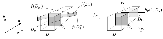
Figure 2: Example of a homotopy from Definition 7 of the covering $D_{\theta}\binrel@{\Longrightarrow}\binrel@@{\mathop{\kern 0.0pt\Longrightarrow}\limits^{f}}D$.

The intuition behind Definition 7 is depicted in Figure 2. There we consider $\Lambda$ to be a circle, and $E^{u}$ and $E^{s}$ to be trivial bundles over $\Lambda$ with real one dimensional fibers; in short, we consider $E=\mathbb{S}^{1}\times\mathbb{R}\times\mathbb{R}$. On the plot, the front and the back sides (i.e. $D_{\theta=0}$ and $D_{\theta=2\pi}$) of the set $D$ are identified to be the same. For the conditions of Definition 7 to hold we need to have topological expansion on the $x$ coordinates. This means that the ‘exit set’ $D_{\theta}^{-}$ will be mapped outside of $D$. In addition, we also need topological contraction on the coordinate $y$. This ensures that $f(D_{\theta})$ will not intersect with $D^{+}$. We impose quite mild conditions on the dynamics on $\theta$. It is enough that the correct topological alignment can be pulled by a homotopy to a fiber $E_{\Theta}$. Note that in Definition 7 we do not require the map to carry fibers into fibers, as is the case in the setting of normal hyperbolicity. Such assumption is not needed for any of our results in this paper.

We now formulate our first main result.

Theorem 8.

If $f:D\rightarrow E$ is a continuous mapping and $D_{\theta}\binrel@{\Longrightarrow}\binrel@@{\mathop{\kern 0.0pt\Longrightarrow}\limits^{f}}D$ holds for every $\theta\in\Lambda$, then for any $\theta\in\Lambda$ there exists a trajectory starting from $D_{\theta}$, which remains in $D$ for all forward iterates, i.e., there exists $v\in D_{\theta}$ such that $f^{m}\left(v\right)\in D$ for all $m\in\mathbb{N}$.

The proof is given in section 6.

Theorem 8 establishes the existence of points that remain in $D$ for all iterates of a map when going forwards in time. Now we turn to what happens also backwards in time. For this we make an additional assumption that $\Lambda$ is a connected manifold.

Definition 9.

Consider a continuous map $f:D\rightarrow E$ (not necessarily invertible). We say that $D$ f-covers $D$, denoted $D\binrel@{\Longrightarrow}\binrel@@{\mathop{\kern 0.0pt\Longrightarrow}\limits^{f}}D$, if the following conditions are satisfied:

1. There exists a homotopy $h:[0,1]\times D\rightarrow E$ such that the following hold true

   $$h(0,\cdot) =f(\cdot),$$

   $$h([0,1]\times D^{-})\cap D =\emptyset,$$ (2)

   $$h([0,1]\times D)\cap D^{+} =\emptyset.$$ (3)

2. There exists a continuous map $\eta:\Lambda\rightarrow\Lambda$ for which

   $$\deg_{2}\left(\eta\right)\neq 0,$$ (4)

   moreover,

   1. If $u>0$, then for any $\theta\in\Lambda$ there exists a linear map $A_{\theta}:E_{\theta}^{u}\rightarrow E_{\eta\left(\theta\right)}^{u}$ such that $A_{\theta}(\partial B_{\theta}^{u})\subset E_{\eta\left(\theta\right)}^{u}\setminus B_{\eta\left(\theta\right)}^{u}$ ($A_{\theta}$ is expanding) and

      $$h(1,\left(\theta;x,y\right))=(\eta\left(\theta\right);A_{\theta}x,0)\in E_{\eta\left(\theta\right)}.$$

   2. If $u=0$, then

      $$h_{\theta}(1,\left(\theta;y\right))=\left(\eta\left(\theta\right);0\right)\in E_{\eta\left(\theta\right)}=E_{\eta\left(\theta\right)}^{s}.$$

      (In the above line we have omitted $x$ from the notation $\left(\theta;x,y\right)$ since $E^{u}$ is of dimension zero.)

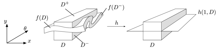
Figure 3: Example of a homotopy from Definition 9 of the covering $D\binrel@{\Longrightarrow}\binrel@@{\mathop{\kern 0.0pt\Longrightarrow}\limits^{f}}D$.

The intuition behind Definition 9 is similar to what we discussed for Definition 7. We need to have topological expansion in $x$ and topological contraction in $y$. In addition, we assume that the dynamics on $\theta$ is homotopic to some map with nonzero degree. Such property is visualized in Figure 3.

We make a couple of remarks before we formulate our second main result.

Remark 10.

Condition $D\binrel@{\Longrightarrow}\binrel@@{\mathop{\kern 0.0pt\Longrightarrow}\limits^{f}}D$ implies that $D_{\theta}\binrel@{\Longrightarrow}\binrel@@{\mathop{\kern 0.0pt\Longrightarrow}\limits^{f}}D$ holds for any $\theta\in\Lambda$. (This follows by taking $h_{\theta}=h|_{\left[0,1\right]\times D_{\theta}}$ and $\Theta=\eta\left(\theta\right)$.) The implication in the other direction is not always true. For instance, when $\pi\circ f(D)=\Theta$, meaning that $f$ maps to a single fiber $E_{\Theta}$, then we can have $D_{\theta}\binrel@{\Longrightarrow}\binrel@@{\mathop{\kern 0.0pt\Longrightarrow}\limits^{f}}D$ for any $\theta\in\Lambda$, but $\eta$ satisfying (4) will not exist.

Remark 11.

Condition (4) is quite natural for stroboscopic (time-shift) maps of flows. In such setting, if the time shift along the flow used to define the map is small enough, then it is possible to find a homotopy to $\eta$ chosen to be the identity on $\Lambda$. Condition (4) is also automatically fulfilled in the setting of normal hyperbolicity; we show this in Lemma 20.

Remark 12.

In (4) we use the degree modulo two of a map. This is because we do not wish to impose any orientablity assumptions. If the considered manifolds $\Lambda$ and $E$ are oriantable, one could use the Brouwer degree instead. Condition (4) can also be replaced by requiring that the degree computed at every point in $\Lambda$ is nonzero (Brouwer degree computed at every point in $\Lambda$ is nonzero, if $\Lambda$ and $E$ are oriantable); for which we do not need $\Lambda$ to be connected. (These generalizations are highlighted in the footnote on page 5 during the proof of Theorem 13.)

We now formulate our second main result:

Theorem 13.

If $f:D\rightarrow E$ is a continuous mapping and $D\binrel@{\Longrightarrow}\binrel@@{\mathop{\kern 0.0pt\Longrightarrow}\limits^{f}}D$, then for every $\theta\in\Lambda$ there exists an orbit in $D$ passing through $D_{\theta}$, i.e., there exists a sequence $\left\{v_{i}\right\}_{i\in\mathbb{Z}}\subset D$, such that $v_{0}\in D_{\theta}$ and $f\left(v_{i}\right)=v_{i+1}$, for all $i\in\mathbb{Z}$.

The proof is given in section 7.

Remark 14.

In Theorems 8 and 13 we obtain sets of points that remain in $D$ for iterates of the single map $f$. We can in fact just as well compose sequences of maps.

To be precise, let $f_{i}:E\to E$ be a sequence of continuous maps and consider a dynamical system

$$v_{i+1}=f_{i}(v_{i}).$$ (5)

Using mirror arguments to those used for the proof of Theorem 8 we can obtain forward trajectories of (5) in $D$ as long as $D_{\theta}\binrel@{\Longrightarrow}\binrel@@{\mathop{\kern 0.0pt\Longrightarrow}\limits^{f_{i}}}D$ for all $i\in\mathbb{N}$ and all $\theta\in\Lambda$.

Similarly, if $D\binrel@{\Longrightarrow}\binrel@@{\mathop{\kern 0.0pt\Longrightarrow}\limits^{f_{i}}}D$ for all $i\in\mathbb{Z}$, then using mirror arguments to those used for the proof of Theorem 13 we can obtain full trajectories of (5) in $D$.

The minor modifications needed for these results are highlighted in the footnotes during the course of the proofs of Theorems 8 and 13 on pages 25 and 7, respectively.

We also have the following continuation results for continuous families of maps, which satisfy the covering condition.

Theorem 15.

Assume that we have a family of maps $f_{\alpha}:D\rightarrow E$, which depends continuously on $\alpha\in\left[0,1\right]$. If for all $\alpha\in\left[0,1\right]$ and all $\theta\in\Lambda,$ $D_{\theta}\binrel@{\Longrightarrow}\binrel@@{\mathop{\kern 0.0pt\Longrightarrow}\limits^{f_{\alpha}}}D$, then for any $\theta\in\Lambda$ there exists a compact connected component $C$ of $\left[0,1\right]\times D_{\theta}$ which meets both $\left\{0\right\}\times D_{\theta}$ and $\left\{1\right\}\times D_{\theta},$ such that for any $\left(\alpha,v\right)\in C$

$$f_{\alpha}^{n}\left(v\right)\in D\mathchoice{\hbox{{ for all }}}{\hbox{{\firstchoice@false for all }}}{\hbox{{\firstchoice@false for all }}}{\hbox{{\firstchoice@false for all }}}n\in\mathbb{N}.$$

The proof is given in section 8.

Theorem 16.

Assume that we have a family of maps $f_{\alpha}:D\rightarrow E$, which depends continuously on $\alpha\in\left[0,1\right]$. If for all $\alpha\in\left[0,1\right]$, $D\binrel@{\Longrightarrow}\binrel@@{\mathop{\kern 0.0pt\Longrightarrow}\limits^{f_{\alpha}}}D$, then for any $\theta\in\Lambda$ there exists a compact connected component $C$ of $\left[0,1\right]\times D_{\theta}$ which meets both $\left\{0\right\}\times D_{\theta}$ and $\left\{1\right\}\times D_{\theta},$ such that for any $\left(\alpha,v\right)\in C$ there exists an orbit of $f_{\alpha}$ in $D$ passing through $v$, i.e., there exists as sequence $\left\{v_{i}\right\}_{i\in\mathbb{Z}}\subset D$, such that $v_{0}=v\in D_{\theta}$ and $f_{\alpha}\left(v_{i}\right)=v_{i+1}$, for all $i\in\mathbb{Z}$.

The proof is given in section 9.

Figure 4: The connected component $C$ from Remark 17.

Remark 17.

We can not assert that $C$ from Theorems 15, 16 is path connected. We can see this if we take $f_{\alpha}:\mathbb{R\rightarrow R}$ with $f_{\alpha}(x)=x+\alpha\left(x-\frac{1}{2}\sin\frac{1}{\alpha}\right)+g\left(x\right),$ where $g:\mathbb{R\rightarrow R}$ is continuous with $g|_{\left[-1/2,1/2\right]}=0$, $g|_{\left\{x>1/2\right\}}>0$ and $g|_{\left\{x<-1/2\right\}}<0$ (see Figure 4). For $\alpha\in(0,1]$ we have a family of hyperbolic fixed points $x_{\alpha}:=\frac{1}{2}\sin\frac{1}{\alpha}$ of $f_{\alpha}$. Assumptions of Theorems 15, 16 hold, since for all $\alpha\in\left[0,1\right]$ the maps $f_{\alpha}$ stretch the interval $D=\left[-1,1\right]$. We can not find a path connecting the set of fixed points $\left[-\frac{1}{2},\frac{1}{2}\right]$ of $f_{0}$ with $x_{\alpha}$. Nevertheless, we see that $C=\left\{0\right\}\times\left[-\frac{1}{2},\frac{1}{2}\right]\cup\left\{\left(\alpha,x_{\alpha}\right)|\,\alpha\in(0,1]\right\}$ is connected (but not path connected).

Remark 18.

In the definition of the set $D$ we fixed the norms to be less than or equal to one. This does not make it less general, since our results will hold in any setting that is homeomorphic to the above.

3.2 Application in the context of normal hyperbolicity.

Below we give a corollary to bridge our results with the theory of NHIMs. Before we proceed, we briefly recall the definition.

Definition 19.

Let $M$ be a smooth manifold and $f:M\rightarrow M$ a diffeomorphism. A manifold $\Lambda\subset M$, invariant under $f$, i.e., $f\left(\Lambda\right)=\Lambda$, is said to be normally hyperbolic if there exist a constant $C>0$, rates $0<\lambda<\mu^{-1}<1$ and a splitting

$$T_{\Lambda}M=T\Lambda\oplus E^{u}\oplus E^{s},$$ (6)

which is invariant under the action of the differential $df$ and such that for $\theta\in\Lambda$

$$x\in E_{\theta}^{u} \iff\left\|df^{i}\left(\theta\right)x\right\|\leq C\lambda^{\left|i\right|}\left\|x\right\|,\qquad i\leq 0,$$ (7)

$$y\in E_{\theta}^{s} \iff\left\|df^{i}\left(\theta\right)y\right\|\leq C\lambda^{i}\left\|y\right\|,\qquad i\geq 0,$$ (8)

$$w\in T_{\theta}\Lambda \iff\left\|df^{i}\left(\theta\right)w\right\|\leq C\mu^{\left|i\right|}\left\|w\right\|,\qquad i\in\mathbb{Z}.$$ (9)

We have the following lemma which states that normal hyperbolicity implies the covering condition.

Lemma 20.

Let $\Lambda$ be a compact normally hyperbolic invariant manifold for a diffeomorphism $f:M\rightarrow M$, and let $k\in\mathbb{N}$ satisfy $k>\log_{\lambda}\frac{1}{C}$. Then there exists a neighborhood $D$ of $\Lambda$ such that $D\binrel@{\Longrightarrow}\binrel@@{\mathop{\kern 0.0pt\Longrightarrow}\limits^{f^{k}}}D.$

The proof is given in section 10.

From Theorem 13 and Lemma 20 we obtain the following corollary.

Corollary 21.

Assume that $\Lambda$ is a compact normally hyperbolic invariant manifold for a diffeomorphism $f:M\rightarrow M$, and assume that $D$ is such that $D\binrel@{\Longrightarrow}\binrel@@{\mathop{\kern 0.0pt\Longrightarrow}\limits^{f^{k}}}D$. Let $f_{\alpha}:M\rightarrow M$ be a family of continuous maps, which depends continuously on $\alpha$. Assume that $f_{0}=f$. Then for $\alpha$ for which

$$D\binrel@{\Longrightarrow}\binrel@@{\mathop{\kern 0.0pt\Longrightarrow}\limits^{f^{k}_{\alpha}}}D,$$ (10)

$\Lambda$ persists as an invariant set of $f_{\alpha}$. Moreover, this set projects surjectively onto $\Lambda$.

Corollary 21 ensures that for a perturbation of $f$ the NHIM will persist as an invariant set. In [Floer] Floer proved a similar result. He has shown that if $f_{\alpha}$ are homeomorphisms which are close enough to $f$, then the NHIM persists along with its cohomology ring. The first difference between our result and Floer’s is that Corollary 21 provides a verifiable condition (10) for the persistence of the NHIM, effectively getting rid of the ‘close enough’ part of the Floer’s statement. (For small $\lambda$ (10) will hold, and for a particular system we can explicitly check for which $\lambda$ (10) will be satisfied.) In our setting, the existence of the NHIM is in fact not even necessary, since (10) alone establishes the existence of the invariant sets. Another difference is that in Corollary 21 it is enough that $f_{\alpha}$ are continuous; we do not need them to be homeomorphisms as is required in [Floer]. Floer proves that the cohomology ring of the invariant set which persists contains the cohomology ring of the original manifold as a subring. We prove that the topology of the original manifold is in a sense ‘preserved’, but in our statement this is expressed by the fact that the invariant set which persists projects surjectively onto the original NHIM. Moreover, we know by Theorem 16 that the invariant manifold ‘continues’ in the sense that the sets for different parameters are linked on each fiber by a compact connected component.

A desirable feature of our result is that the covering condition (10) can be checked using computer assisted techniques, which makes our results applicable in practice.

From Remark 14 and Lemma 20 we also obtain the following result for random perturbations of NHIMs. (See [Bates] for a similar persistence result of NHIMs for random perturbations of flows.)

Corollary 22.

Let $\Lambda$ be a compact normally hyperbolic invariant manifold for a diffeomorphism $f:M\rightarrow M$, and let $k\in\mathbb{N}$ satisfy $k>\log_{\lambda}\frac{1}{C}$. Assume that $D$ is such that $D\binrel@{\Longrightarrow}\binrel@@{\mathop{\kern 0.0pt\Longrightarrow}\limits^{f^{k}}}D.$ Let $(\Omega,\mathcal{F},\mathbb{P})$ be a probability space, let $T:\Omega\rightarrow\Omega$ and let $\phi:\mathbb{Z}\times\Omega\times M\rightarrow M$ be a random dynamical system over $T$, i.e. $\phi\left(0,\omega\right)=Id$ and

$$\phi(n+m,\omega)=\phi(n,T^{m}(\omega))\phi\left(m,\omega\right).$$

If $\phi$ is close enough to $f$ so that for any $\omega\in\Omega$, $D\binrel@{\Longrightarrow}\binrel@@{\mathop{\kern 0.0pt\Longrightarrow}\limits^{\phi(k,\omega)}}D,$ then the NHIM persists as a set of trajectories of $\phi$. Moreover, the set projects surjectively onto $\Lambda$.

4 Examples of application.

The perturbations of a system with a NHIM can be such that the perturbed maps are no longer normally hyperbolic, but we can still apply our results. Below we give an example of such a system.

4.1 Toy example

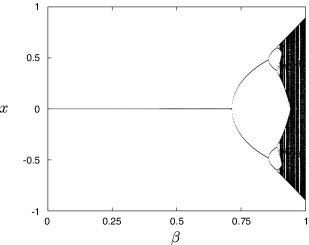
Figure 5: The projection onto the $x$ coordinate of the invariant set from the example from section 4, depending on the parameter $\beta$.

We start with an example where the dynamics on the unstable coordinate is decoupled from the rest of the coordinates. The aim is to provide a simple model on which we can demonstrate some features, without having to engage in computations.

Let $\Lambda$ be a one dimensional circle, parameterized by $\theta\in[0,2\pi)$. Let $E^{u}$ be a trivial bundle over $\Lambda$ (i.e., $E^{u}=\Lambda\times\mathbb{R}$), let $E^{s}$ be a Möbius bundle over $\Lambda$, and let $E=E^{u}\oplus E^{s}$. Take $\mu\in\mathbb{R}$, $|\mu|<\frac{1}{2}$, and two maps $f_{0},f_{1}:E\rightarrow E$ defined as

$$f_{0}\left(\theta;x,y\right) =\left(3\theta\,\mathrm{mod}\,2\pi;4x,\mu y\right),$$

$$f_{1}\left(\theta;x,y\right) =\left(3\theta\,\mathrm{mod}\,2\pi;-3x+5x^{3},\frac{1}{2}\sin\theta+\mu y\right).$$ (11)

The maps $f_{0}$ and $f_{1}$ expand the Möbius strip along $\theta$, wrapping it around itself three times, and squeeze it along the $y$ coordinate (see Figure 6). On the $x$ coordinate we have decoupled dynamics.

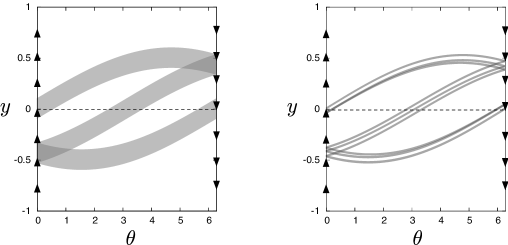
Figure 6: The image of $f_{1}(D)$ (left) and $(f_{1})^{2}(D)$ (right), for the map $f_{1}$ defined in (11) from the example from section 4, projected onto the Möbius bundle $E^{s}$. On the plot, the vertical edge $\{\theta=0\}$ is identified with the vertical edge $\{\theta=2\pi\}$ with reversed sign (which is indicated by arrows on the plots). Here we took $\mu=\frac{1}{10}$ in (11).

In this example we will discuss invariant sets for a family of maps $f_{\beta}:E\rightarrow E$, defined as

$$f_{\beta}:=\left(1-\beta\right)f_{0}+\beta f_{1},\qquad\mathchoice{\hbox{{for }}}{\hbox{{\firstchoice@false for }}}{\hbox{{\firstchoice@false for }}}{\hbox{{\firstchoice@false for }}}\beta\in\left[0,1\right].$$

For $\beta=0$ the set $\left\{x=y=0\right\}$ is invariant, and on it the rate conditions hold; i.e. the dynamics in the hyperbolic directions $x,y$ is stronger than on $\theta$. As we increase $\beta$, the expansion along $x$ becomes weaker than the expansion along $\theta$. This means that the classical tools can not ensure that the manifold survives. If we take though $D=\left\{\left(\theta;x,y\right)|\;\left|x\right|\leq 1,\ \left|y\right|\leq 1\right\}$, fix $\beta\in[0,1]$, consider a homotopy

$$h\left(\alpha,\left(\theta;x,y\right)\right)=\left(1-\alpha\right)f_{\beta}\left(\theta;x,y\right)+\alpha\left(3\theta\,\mathrm{mod}\,2\pi;2x,0\right),$$

and $\eta(\theta)=3\theta\,\mathrm{mod}\,2\pi$, then it is a simple exercise to verify that

$$D\binrel@{\Longrightarrow}\binrel@@{\mathop{\kern 0.0pt\Longrightarrow}\limits^{f_{\beta}}}D.$$ (12)

The reason why (12) holds boils down to the fact that on the $y$ coordinate we have contraction and the cubic terms on the coordinate $x$ ensure expansion away from zero. Since $\eta\left(\theta\right)=3\theta\,\mathrm{mod}\,2\pi$, we see that $\deg_{2}\left(\eta\right)=1$.

Theorem 13 ensures that for any $\beta\in\left[0,1\right]$ there is an invariant set in $D$, with trajectories in $D$ passing through each $\theta\in[0,2\pi)$. Theorem 13 does not claim that the invariant set is a manifold. In fact it is not a manifold, which we can see if we look at the projections in Figures 5 and 6. Figure 5 contains the plot of the invariant set of $x\mapsto\pi^{u}\circ f_{\beta}\left(\theta;x,y\right)$ for $\beta\in\left[0,1\right]$. (The dynamics of $f_{\beta}$ on $x$ is decoupled from other variables, so the set is independent from the choice of $\theta,y$.) We see that for $\beta$ close to 1 our set will be chaotic. This is because the function passes through logistic type bifurcations as we increase $\beta$. In Figure 6 we take the parameter $\mu=\frac{1}{10}$, fix $\beta=1$ and plot the projections of $f_{\beta}\left(D\right)$ and $f_{\beta}^{2}\left(D\right)$ onto the Möbius strip. We see that if we were to consider $f_{\beta}^{k}\left(D\right)$ for higher $k$, then we would see the emergence of a Cantor structure of our invariant set. Theorem 16 states that the resulting invariant set for different $\beta$ ‘continues’ as the parameter changes, which we see is the case in our example.

The main feature of this example is that we have started with a manifold which satisfied the rate conditions, and perturbed the system into the parameter range where the rate conditions fail. Nevertheless, our method establishes the existence of an invariant set for all parameters.

In our example the dynamics on $x$ is decoupled from the dynamics on the Möbius bundle. We have done this for simplicity. The assumptions of Theorems 13, 16 are robust under small perturbations, so we will also obtain the results for any map that is appropriately close to $f_{\beta}$, for one of the $\beta\in\left[0,1\right].$

In our example we were able to verify (4) because $f_{\beta}$ on coordinate $\theta$ were given as $3\theta\,\mathrm{mod}\,2\pi$. If we were to take $k\theta\,\mathrm{mod}\,2\pi$ with an even number $k$, then we would get $\deg\left(\eta\right)=0$, and we would not be able to apply Theorem 13. We finish by observing that in such a setting we can still use Theorem 8 to obtain an invariant set of points that stay in $D$ for all (forward) iterations.

The above was just a toy example. Similar features though can be found for instance in the Kuznetsov system (see [Kuzn, Wilczak]), where we have a hyperbolic invariant set in $\mathbb{R}^{3}$, which has a Cantor set structure.

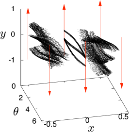
Figure 7: The invariant set of (13).

4.2 An example with a computer assisted proof

Here we modify our example from section 13 by coupling the dynamics between the coordinates. We consider the following map

$$f\left(\theta;x,y\right)=$$ (13)

$$\left(3\theta+xy\sin(\theta)\mathchoice{\hbox{{ }}}{\hbox{{\firstchoice@false }}}{\hbox{{\firstchoice@false }}}{\hbox{{\firstchoice@false }}}\mathrm{mod}\mathchoice{\hbox{{ }}}{\hbox{{\firstchoice@false }}}{\hbox{{\firstchoice@false }}}{\hbox{{\firstchoice@false }}}2\pi;4x^{3}-\frac{8}{5}x+\frac{1}{2}xy,\mu y+\frac{2}{5}\sin\theta+x\cos(\theta)\right),$$

with $\mu=1/10.$ This map results from taking $f_{\beta}$ from the previous section with $\beta=0.8$, and by adding the coupling terms $xy\sin(\theta)$, $\frac{1}{2}xy$ and $x\cos(\theta)$ to the $\theta$-, $x$- and $y$-coordinates, respectively. The choice of such coupling was to a large extent arbitrary. We wanted a nontrivial but simple example, with some interesting features.

In Figure 7 we give the plot of a numerically obtained representation of the invariant set we will establish. On the plot, the front face $\theta=2\pi$ is identified with the back face $\theta=0$, but should be glued together according to the arrows to take into account the fact that $E_{s}$ is a Mobius bundle.

For $x=0$ we see the invariant set from our previous example (compare Figures 6 and 7); we have intentionally chosen our coupling to preserve it. The coupling is strong enough to distort the two attracting fixed points of the uncoupled map $f_{\beta=0.8}$ on $x$ (See Figure 5) to become the two ‘chaotic clouds’ from Figure 7.

For this example we provide a computer assisted proof that for $D=\left\{\left(\theta;x,y\right):\left\|x\right\|\leq 1,\left\|y\right\|\leq 1.2\right\}$ we will have $D\binrel@{\Longrightarrow}\binrel@@{\mathop{\kern 0.0pt\Longrightarrow}\limits^{f}}D$, which, by Theorem 13, implies the existence of an invariant set in $D$. This is done by considering the following homotopy

$$h\left(\alpha,\left(\theta;x,y\right)\right):= (3\theta+\left(1-\alpha\right)xy\sin(\theta)\mathchoice{\hbox{{ }}}{\hbox{{\firstchoice@false }}}{\hbox{{\firstchoice@false }}}{\hbox{{\firstchoice@false }}}\mathrm{mod}\mathchoice{\hbox{{ }}}{\hbox{{\firstchoice@false }}}{\hbox{{\firstchoice@false }}}{\hbox{{\firstchoice@false }}}2\pi;$$

$$\alpha 2x+\left(1-\alpha\right)\left(4x^{3}-\frac{8}{5}x+\frac{1}{2}xy\right),$$

$$\left(1-\alpha\right)\left(\mu y+\frac{2}{5}\sin\theta+x\cos(\theta)\right)).$$

Condition (4) follows directly from the definition of $h$. We validate (2–3) by using interval arithmetic. Interval arithmetic involves enclosing numbers in intervals that account for possible round-off errors, and performing arithmetic operation on these intervals. The output of these operations are intervals, which account for the numerical error and enclose the true result.

We give the full code which we have used for our computer assisted proof in B and follow with a number of comments associated to the particular routines. The validation of (2–3) is based on subdividing the domains into small sets and checking the correct topological alignment by means of inequalities between intervals. A sample of such bounds obtained by our computer program is depicted in Figure 8.

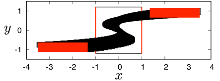
Figure 8: A sample of computations performed by the computer. We subdivide $D$ into small cubes, and check inequalities which ensure that local projections onto $x,y$ do not intersect with $D^{+}$. We also compute images of cubes from $D^{-}$ (in red) and check that they map to the left and to the right of the set $D$.

4.3 Finding invariant sets and covering relations

If the system under consideration possesses a NHIM, then it is a natural choice to position $D$ around the NHIM, aligning $D^{+}$ and $D^{-}$ with the stable and unstable bundles, respectively. When the perturbation is far from the normally hyperbolic case, or if we want to apply our methods in a setting where no NHIM exists, we can use the following numerical method.

We can select some domain within which we expect to find our invariant object, and subdivide it into cubes. Then, using interval arithmetic we can propagate such cubes and discard those that will leave the domain after some iterate of the map. Those cubes that do not escape are dissected into smaller cubes, and the procedure can be repeated. If some invariant set is within our domain, it will be detected by this method.

The reason for using interval arithmetic is that even if just a single point from a considered cube is an element of the invariant object, then it will not leave the domain, and the cube will not be discarded. (For instance, the discussed methodology works very well in the normally hyperbolic setting, to find an enclosure of the stable manifold.)

The positioning of the enclosure that comes out of the algorithm can give an insight into how $D^{+}$ and $D^{-}$ should be positioned. In Figure 9 we show an outcome of the procedure applied to the map (13) for domains of the form $\{(\theta;x,y):x^{2}+y^{2}<r^{2}\}$, for $r=2$ and $r=1/2$. (On the plot we depict cubes with $\theta=\pi/3$, because we took a liking to the shape on the right hand side.) For $r=2$ we see that $D^{+}$ should be towards the vertical and $D^{-}$ towards the horizontal axis. For $r=1/2$ though we obtain an enclosure that does not give a clear indication how $D^{+}$ and $D^{-}$ could be positioned. Finding suitable $D$ in complicated systems is not an easy task and is likely to involve trial and error.

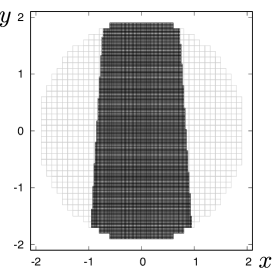
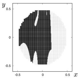
Figure 9: In grey is the set of initial cubes containing $\theta=\pi/3$ at the start of our algorithm. The left plot is for $r=2$ and the right for $r=1/2$. The black cubes are those left after two steps of the procedure.

5 Embedding into reals

In this section we shall embed $E$ in $\mathbb{R}^{N}$. We will then extend the map $f$ so that it is defined on a set with nonempty interior in $\mathbb{R}^{N}$. Such embedding will be useful for us since to find two points $v_{1},v_{2}\in D$ such that $v_{2}=f(v_{1})$ we will be able to do so more easily by embedding $f(v_{1})$ and $v_{2}$ into $\mathbb{R}^{N}$, computing their difference, and solving for zero. Searching for zeros in $\mathbb{R}^{N}$ is more tractable than finding two points on a vector bundle that map one into the other.

The vector bundle $E$ is an $n$-dimensional smooth manifold, $n=c+u+s$. By the Whitney embedding theorem [Whitney] there exists a smooth embedding $\omega:E\rightarrow\mathbb{R}^{2n}$. Let $N_{w}\left(\omega\left(E\right)\right)\mathbf{\subset}\mathbb{R}^{2n}$ stand for the normal space to the manifold $\omega\left(E\right)$ in $\mathbb{R}^{2n}$ at $w\in\omega\left(E\right)$. (Since $\omega\left(E\right)$ is a manifold of dimension $n$, the dimension of $N_{w}\left(\omega\left(E\right)\right)$ is $n$.) We consider the tubular neighborhood of $\omega\left(E\right)$

$$\mathcal{T}:=\left\{w+z|\;w\in\omega\left(E\right),\ z\in N_{w}\left(\omega\left(E\right)\right),\ \left\|z\right\|_{\mathbb{R}^{2n}}\leq\delta\left(w\right)\right\}\subset\mathbb{R}^{2n},$$ (15)

where $\delta:\omega\left(E\right)\rightarrow\mathbb{R}_{+}$ is continuous. Let us abuse the notation slightly by introducing a number $\delta\in\mathbb{R}$ defined as

$$\delta:=\min_{w\in\omega\left(D\right)}\delta\left(w\right).$$ (16)

Since $D$ is compact $\delta>0$ is well defined.

Notation 23.

For $v\in E$ we shall write a pair $\left(v,z\right)$ to represent a point $\omega\left(v\right)+z\in\mathcal{T}$. In this convention writing the pair $\left(v,z\right)$ implies that $z\in N_{\omega\left(v\right)}\left(\omega\left(E\right)\right).$ In the same way by writing $\left(\theta;x,y,z\right)$ we mean the point $\omega\left(\theta;x,y\right)+z\in\mathcal{T}$, and imply that $z\in N_{\omega\left(\theta;x,y\right)}\left(\omega\left(E\right)\right).$

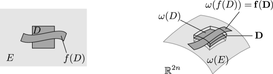
Figure 10: Depiction of our embedding. The set $\mathbf{D}$ is a tubular neighborhood of $\omega(D)$. The map $\mathbf{f}$ defined on $\mathbf{D}$ contracts in the normal direction onto $\omega(f(D))$. This means that the normal direction is treated as an additional contracting coordinate.

Using Notation 23 we define the following subsets of $\mathbb{R}^{2n}$

$$\mathbf{D}:=\left\{\left(v,z\right)\in\mathcal{T}|\;v\in D,\ \left\|z\right\|_{\mathbb{R}^{2n}}\leq\delta\right\},$$ (17)

$$\mathbf{D}_{\theta}:=\mathbf{D}\cap\left\{\left(v,z\right)|\;\pi\left(v\right)=\theta\right\},\qquad\mathbf{D}_{U}:=\bigcup_{\lambda\in U}\mathbf{D}_{\lambda}.$$

We define a map

$$\mathbf{f}:\mathbf{D}\rightarrow\mathbb{R}^{2n},$$

as

$$\mathbf{f}\left(v,z\right):=\left(f\left(v\right),0\right),$$ (18)

where the zero on the right hand side is on the $z$-coordinate. (In other words, $\mathbf{f}(\omega\left(v\right)+z)=\omega\left(f\left(v\right)\right)$; see Figure 10.) If we need to include more detail, using also the convention of Notation 23, we can write

$$\mathbf{f}\left(\theta;x,y,z\right)=\left(f\left(\theta;x,y\right),0\right),$$

where the zero on the right hand side is on the $z$-coordinate. Observe that directly from the definition of $\mathbf{f}$ we have the following:

Lemma 24.

If for $\left(v_{1},z_{1}\right),\left(v_{2},z_{2}\right)\in\mathcal{T}$ we have $\left(v_{2},z_{2}\right)=\mathbf{f}\left(v_{1},z_{1}\right)$, then $v_{2}=f\left(v_{1}\right)$.

Proof.

By definition, $\left(v_{2},z_{2}\right)=\mathbf{f}\left(v_{1},z_{1}\right)$ implies $\omega\left(f\left(v_{1}\right)\right)=\omega\left(v_{2}\right)+z_{2}$. Since $\mathcal{T}$ is a tubular neighborhood of $\omega\left(E\right)$, each point in $\mathcal{T}$ is represented in a unique way as $\omega\left(v\right)+z$. This means that $\omega\left(f\left(v_{1}\right)\right)=\omega\left(v_{2}\right)+z_{2}$ implies that $z_{2}=0$ and $\omega\left(f\left(v_{1}\right)\right)=\omega\left(v_{2}\right),$ which in turn gives $f\left(v_{1}\right)=v_{2}$, as required. ∎

Remark 25.

When we looking for two points $v_{1},v_{2}\in D$ such that $v_{2}=f(v_{1})$, by Lemma 24 we can solve

$$\mathbf{f}\left(v_{1},z_{1}\right)-\left(v_{2},z_{2}\right)=0,$$ (19)

for $\left(v_{1},z_{1}\right),\left(v_{2},z_{2}\right)\in\mathbf{D}$. (In (19) we are subtracting two vectors in $\mathbb{R}^{2n}$.)

6 Proof of Theorem 8

Proof.

Let us fix $\theta=\Theta_{0}\in\Lambda$. Our objective will be to find a trajectory starting from $D_{\Theta_{0}}$, which remains in $D$ for all forward iterates. We start by finding trajectories of length $k$.

Let $0^{2n}$ denote zero in $\mathbb{R}^{2n}.$ For fixed $k\in\mathbb{N}$ we consider the following sets (recall that $\mathbf{D}$ was defined in (17))

$$\overline{X} :=D_{\Theta_{0}}^{u}\times\binrel@{\underbrace{\mathbf{D}\times\ldots\times\mathbf{D}}}\binrel@@{\mathop{\kern 0.0pt\underbrace{\mathbf{D}\times\ldots\times\mathbf{D}}}\limits_{k}},$$ (20)

$$Y :=\binrel@{\underbrace{\mathbb{R}^{2n}\times\ldots\times\mathbb{R}^{2n}}}\binrel@@{\mathop{\kern 0.0pt\underbrace{\mathbb{R}^{2n}\times\ldots\times\mathbb{R}^{2n}}}\limits_{k}}\times E,$$ (21)

$$Z :=\binrel@{\underbrace{\{0^{2n}\}\times\ldots\times\{0^{2n}\}}}\binrel@@{\mathop{\kern 0.0pt\underbrace{\{0^{2n}\}\times\ldots\times\{0^{2n}\}}}\limits_{k}}\times\left\{\left(\theta;0,y\right)|\;\theta\in\Lambda,\ \left\|y\right\|_{s}<1\right\}.$$ (22)

We consider $\overline{X}$ as a subset of $E_{\Theta_{0}}^{u}\times\mathcal{T}\times\ldots\times\mathcal{T}$, so

$$X=\mathrm{int}\overline{X}=\mathrm{int}D_{\Theta_{0}}^{u}\times\binrel@{\underbrace{\mathrm{int}\mathbf{D}\times\ldots\times\mathrm{int}\mathbf{D}}}\binrel@@{\mathop{\kern 0.0pt\underbrace{\mathrm{int}\mathbf{D}\times\ldots\times\mathrm{int}\mathbf{D}}}\limits_{k}}.$$

Note that since $\Lambda$ is compact so is $\overline{X}$. $Y$ is a manifold without boundary and $Z$ is its submanifold, with

$$\overline{Z} =\{0^{2n}\}\times\ldots\times\{0^{2n}\}\times\left\{\left(\theta;0,y\right)|\;\theta\in\Lambda,\ \left\|y\right\|_{s}\leq 1\right\},$$ (23)

$$\partial Z =\{0^{2n}\}\times\ldots\times\{0^{2n}\}\times\left\{\left(\theta;0,y\right)|\;\theta\in\Lambda,\ \left\|y\right\|_{s}=1\right\}.$$ (24)

The manifolds $X$ and $Z$ are of complementary dimension with respect to $Y$:

$$\dim X=u+2kn,\qquad\dim Z=c+s,\qquad\dim Y=2kn+n.$$

To show the existence of an orbit of length $k$ in $D$ we consider a map

$$F=\left(F_{1},\ldots,F_{k},F_{k+1}\right):\overline{X}\rightarrow Y,$$

which is defined as follows. For

$$\mathbf{x}=\left(\left(\Theta_{0};x_{0}\right),\left(\theta_{1};x_{1},y_{1},z_{1}\right),\ldots,\left(\theta_{k};x_{k},y_{k},z_{k}\right)\right)\in\overline{X}$$ (25)

we define (recall that $\mathbf{f}$ was defined in (18))

$$F_{1}\left(\mathbf{x}\right) :=\mathbf{f}\left(\Theta_{0};x_{0},0,0\right)-\left(\theta_{1};x_{1},y_{1},z_{1}\right),$$

$$F_{2}\left(\mathbf{x}\right) :=\mathbf{f}\left(\theta_{1};x_{1},y_{1},z_{1}\right)-\left(\theta_{2};x_{2},y_{2},z_{2}\right),$$ (26)

$$\;\;\;\vdots$$

$$F_{k}\left(\mathbf{x}\right) :=\mathbf{f}\left(\theta_{k-1};x_{k-1},y_{k-1},z_{k-1}\right)-\left(\theta_{k};x_{k},y_{k},z_{k}\right),$$

$$F_{k+1}\left(\mathbf{x}\right) :=f\left(\theta_{k};x_{k},y_{k}\right).$$

Our objective will be to prove that there exists an $\mathbf{x\in}\overline{X},$ such that

$$F\left(\mathbf{x}\right)\in Z.$$ (27)

Observe that by Lemma 24, (27) establishes the existence of a trajectory of $f:D\rightarrow E,$ that starts in $v=\left(\Theta_{0};x_{0},0\right)$ and remains in $D$ for $k$ iterates of $f$:

$$f^{i}\left(v\right)\in D\qquad\mathchoice{\hbox{{for }}}{\hbox{{\firstchoice@false for }}}{\hbox{{\firstchoice@false for }}}{\hbox{{\firstchoice@false for }}}i=1,\ldots,k.$$

Our plan is to establish (27) by showing that the intersection number $I_{2}\left(F,X,Z\right)=1$; then (27) will follow from the intersection property.

The first thing to show is that $F$ is admissible (in the sense of Definition 4). We shall consider an $\mathbf{x}$ of the form (25) which lies in the boundary $\partial X$ and show that $F\left(\mathbf{x}\right)\notin\overline{Z}$. There are several possibilities how $\mathbf{x}$ can lie on $\partial X$, which we will consider one by one below. In the following argument we make use of the fact that $f\left(\theta;x,y\right)=h_{\theta}\left(0,\left(\theta;x,y\right)\right)$, which means that all properties of $h_{\theta}$ from Definition 7 hold for $f$.

The first possibility how $\mathbf{x}$ can lie on $\partial X$ is that $\left\|x_{0}\right\|_{u}=1$. In this case, $\left(\Theta_{0};x_{0},0\right)\in D_{\Theta_{0}}^{-}$, and by the first condition from Definition 7 we know that $f\left(\Theta_{0};x_{0},0\right)\cap D=\emptyset$, so $\mathbf{f}\left(\Theta_{0};x_{0},0,0\right)=\left(f\left(\Theta_{0};x_{0},0\right),0\right)\notin\mathbf{D}$, hence $F_{1}\left(\mathbf{x}\right)\neq 0$, so in turn $F\left(\mathbf{x}\right)\notin\overline{Z}$.

The second way that $\mathbf{x}$ can lie on $\partial X$ is that $\left\|x_{i}\right\|_{u}=1$ for some $i\in\left\{1,\ldots,k-1\right\}$. Then $\left(\theta_{i};x_{i},y_{i}\right)\in D_{\theta_{i}}^{-}$, and also from condition one of Definition 7 we have $f\left(\theta_{i};x_{i},y_{i}\right)\notin D$ so $\mathbf{f}\left(\theta_{i};x_{i},y_{i},z_{i}\right)=\left(f\left(\theta_{i};x_{i},y_{i}\right),0\right)\notin\mathbf{D}$. This means that $F_{i+1}\left(\mathbf{x}\right)\neq 0$, hence $F\left(\mathbf{x}\right)\notin\overline{Z}$.

If $\mathbf{x}$ lies in $\partial X$ because $\left\|x_{k}\right\|_{u}=1$, then $\left(\theta_{k};x_{k},y_{k}\right)\in D_{\theta_{i}}^{-}$ and from Definition 7 we see that $F_{k+1}\left(\mathbf{x}\right)=f\left(\theta_{k};x_{k},y_{k}\right)\notin D,$ hence $F\left(\mathbf{x}\right)\notin\overline{Z}$.

Another possibility for $\mathbf{x}$ to be in $\partial X$ is to have $\left\|y_{i}\right\|_{s}=1$ for some $i\in\left\{1,\ldots,k\right\}$. From Definition 7 it follows that $f\left(D\right)\cap D^{+}=\emptyset$. We see that since $\left\|y_{i}\right\|_{s}=1$ we have $F_{i}\left(\mathbf{x}\right)=\left(f\left(\theta_{i-1};x_{i-1},y_{i-1}\right),0\right)-\left(\theta_{i};x_{i},y_{i},z_{i}\right)\neq 0$ (where $y_{0}=0$), so $F\left(\mathbf{x}\right)\notin\overline{Z}$.

The last possibility for $\mathbf{x}$ to be on $\partial X$ is that $\left\|z_{i}\right\|_{\mathbb{R}^{2n}}=\delta$ for some $i\in\left\{1,\ldots,k\right\}$, then $F_{i}\left(\mathbf{x}\right)=\left(f\left(\theta_{i-1};x_{i-1},y_{i-1}\right),0\right)-\left(\theta_{i};x_{i},y_{i},z_{i}\right)\neq 0$, so $F\left(\mathbf{x}\right)\notin\overline{Z}$.

Above we have shown that

$$F\left(\partial X\right)\cap\overline{Z}=\emptyset.$$ (28)

We now need to show that

$$F\left(\overline{X}\right)\cap\partial Z=\emptyset.$$ (29)

If $\mathbf{y}\in\partial Z$, then

$$\mathbf{y}=\left(0,\ldots,0,\left(\theta;0,y\right)\right)\quad\mathchoice{\hbox{{for some }}}{\hbox{{\firstchoice@false for some }}}{\hbox{{\firstchoice@false for some }}}{\hbox{{\firstchoice@false for some }}}\theta\in\Lambda,\mathchoice{\hbox{{ and }}}{\hbox{{\firstchoice@false and }}}{\hbox{{\firstchoice@false and }}}{\hbox{{\firstchoice@false and }}}\;\left\|y\right\|_{s}=1.$$ (30)

Since $F_{k+1}\left(\mathbf{x}\right):=f\left(\theta_{k};x_{k},y_{k}\right)$ and from Definition 7 it follows that $f\left(D\right)\cap D^{+}=\emptyset$, we see that $F_{k+1}\left(\mathbf{x}\right)\neq\mathbf{y.}$ We have shown (29), thus $F$ is admissible.

Our objective will now be to construct an admissible (in the sense of Definition 5) homotopy from $F$ to some map that is transversal to $Z$. We will do this in a number of steps, by constructing several admissible homotopies and then gluing them together. A less patient reader might want to take a peek at (45), where we write out the map we make the homotopy to. Looking at (45) will give an idea of our final objective.

Our first homotopy will be denoted as

$$H^{\left(1\right)}=\left(H_{1}^{\left(1\right)},\ldots,H_{k}^{\left(1\right)},H_{k+1}^{\left(1\right)}\right):\left[0,1\right]\times\overline{X}\rightarrow Y.$$

Since $D_{\Theta_{0}}\binrel@{\Longrightarrow}\binrel@@{\mathop{\kern 0.0pt\Longrightarrow}\limits^{f}}D$, we can take the homotopy $h_{\Theta_{0}}$ from Definition 7, and for $\mathbf{x}$ of the form (25) we can define

$$H_{1}^{\left(1\right)}\left(\alpha,\mathbf{x}\right) :=\left(h_{\Theta_{0}}\left(\alpha,\left(\Theta_{0};x_{0},0\right)\right),0\right)-\left(\theta_{1};x_{1},y_{1},z_{1}\right),$$

$$H_{i}^{\left(1\right)}\left(\alpha,\mathbf{x}\right) :=F_{i}\left(\mathbf{x}\right)\qquad\mathchoice{\hbox{{for }}}{\hbox{{\firstchoice@false for }}}{\hbox{{\firstchoice@false for }}}{\hbox{{\firstchoice@false for }}}i\neq 1.$$

Our homotopy is such that

$$H^{\left(1\right)}\left(0,\mathbf{x}\right)=F\left(\mathbf{x}\right),$$

and for some $\Theta_{1}\in\Lambda$ and linear $A_{0}:E_{\Theta_{0}}^{u}\rightarrow E_{\Theta_{1}}^{u}$ ($\Theta_{1}$ and $A_{0}$ follow from Definition 7)

$$H_{1}^{\left(1\right)}\left(1,\mathbf{x}\right)=\left(\Theta_{1};A_{0}x_{0},0,0\right)-\left(\theta_{1};x_{1},y_{1},z_{1}\right).$$

We need to show that $H^{\left(1\right)}$ is admissible. This will follow from an analogous argument to the one used to prove (28–29). We first need to show that

$$H^{\left(1\right)}\left(\alpha,\mathbf{x}\right)\cap\overline{Z}=\emptyset\quad\mathchoice{\hbox{{for }}}{\hbox{{\firstchoice@false for }}}{\hbox{{\firstchoice@false for }}}{\hbox{{\firstchoice@false for }}}\mathbf{x}\in\partial X\mathchoice{\hbox{{ and }}}{\hbox{{\firstchoice@false and }}}{\hbox{{\firstchoice@false and }}}{\hbox{{\firstchoice@false and }}}\alpha\in\left[0,1\right].$$ (31)

We have already established (28) and we know that for $i\neq 1,$ by definition, $H_{i}^{\left(1\right)}\left(\alpha,\mathbf{x}\right)=F_{i}\left(\mathbf{x}\right)$. This means that to check (31) it is enough to consider three cases. The first is that $\mathbf{x}\in\partial X$ is such that $\left\|x_{0}\right\|_{u}=1$. The second case $\left\|y_{1}\right\|_{s}=1$. The third is $\left\|z_{1}\right\|_{\mathbb{R}^{2n}}=\delta$. (For all other $\mathbf{x}\in\partial X$ condition (31) follows from (28).) In the first case $\left(\Theta_{0};x_{0},0\right)\in D_{\Theta_{0}}^{-}$ so since $h_{\Theta_{0}}\left(\alpha,D_{\Theta_{0}}^{-}\right)\cap D=\emptyset$ we obtain

$$H_{1}^{\left(1\right)}\left(\alpha,\mathbf{x}\right)=\left(h_{\Theta_{0}}\left(\alpha,\left(\Theta_{0};x_{0},0\right)\right),0\right)-\left(\theta_{1};x_{1},y_{1},z_{1}\right)\neq 0,$$ (32)

hence $H^{\left(1\right)}\left(\alpha,\mathbf{x}\right)\notin\overline{Z}$. For the second case, since $h_{\Theta_{0}}\left(\alpha,D_{\Theta_{0}}\right)\cap D^{+}=\emptyset$ also ensures (32), we have $H^{\left(1\right)}\left(\alpha,\mathbf{x}\right)\notin\overline{Z}$. If $\left\|z_{1}\right\|=\delta$ then we also see that (32) holds. We have thus established (31). The fact that

$$H^{\left(1\right)}\left(\left[0,1\right]\times\overline{X}\right)\cap\partial Z=\emptyset$$ (33)

follows from (29). (This is because $H^{(1)}_{k+1}=F_{k+1}$, and $F_{k+1}$ was used to establish (29).) This means that we have established that $H^{\left(1\right)}$ is admissible.

Since $H^{\left(1\right)}$ is admissible and $H^{\left(1\right)}\left(0,\cdot\right)=F$, from the homotopy property of the intersection number we obtain

$$I_{2}\left(F,X,Z\right)=I_{2}\left(H^{\left(1\right)}\left(0,\cdot\right),X,Z\right)=I_{2}\left(H^{\left(1\right)}\left(1,\cdot\right),X,Z\right).$$ (34)

Before specifying the next homotopy we shall make use of the excision property. For this we take a closed set $U_{\Theta_{1}}\subset\Lambda$ such that $\mathrm{int}U_{\Theta_{1}}\neq\emptyset$ and $\Theta_{1}\in\mathrm{int}U_{\Theta_{1}}$. We can take $U_{\Theta_{1}}$ small enough so that it is in the domain of some trivialization of $E$ and so that it is contractible to the point $\Theta_{1}$. Let us denote such a continuous contraction by $g_{\Theta_{1}}:\left[0,1\right]\times U_{\Theta_{1}}\rightarrow U_{\Theta_{1}}$ for which $g_{\Theta_{1}}\left(0,\theta\right)=\theta$ and $g_{\Theta_{1}}\left(1,\theta\right)=\Theta_{1}$. We now define a set $\overline{X^{\left(1\right)}}\subset\overline{X}$ as

$$\overline{X^{\left(1\right)}}=D_{\Theta_{0}}^{u}\times\mathbf{D}_{U_{\Theta_{1}}}\times\binrel@{\underbrace{\mathbf{D}\times\ldots\times\mathbf{D}}}\binrel@@{\mathop{\kern 0.0pt\underbrace{\mathbf{D}\times\ldots\times\mathbf{D}}}\limits_{k-1}}.$$

We see that

$$X^{\left(1\right)}=\mathrm{int}\overline{X^{\left(1\right)}}=\mathrm{int}D_{\Theta_{0}}^{u}\times\mathrm{int}\mathbf{D}_{U_{\Theta_{1}}}\times\binrel@{\underbrace{\mathrm{int}\mathbf{D}\times\ldots\times\mathrm{int}\mathbf{D}}}\binrel@@{\mathop{\kern 0.0pt\underbrace{\mathrm{int}\mathbf{D}\times\ldots\times\mathrm{int}\mathbf{D}}}\limits_{k-1}}.$$

We will use the excision property to restrict $H^{\left(1\right)}\left(1,\cdot\right)$ from $X$ to $X^{\left(1\right)}$. For this we first need to show that

$$H^{\left(1\right)}\left(1,X\right)\cap Z=H^{\left(1\right)}\left(1,X^{\left(1\right)}\right)\cap Z.$$ (35)

If we take some $\mathbf{x\in}X\setminus X^{\left(1\right)}$ of the form (25), then $\theta_{1}\notin\mathrm{int}U_{\Theta_{1}}$, so in particular $\theta_{1}\neq\Theta_{1}$. This means that

$$H_{1}^{\left(1\right)}\left(1,\mathbf{x}\right)=\left(\Theta_{1};A_{0}x_{0},0,0\right)-\left(\theta_{1};x_{1},y_{1},z_{1}\right)\neq 0,$$

which implies (35). To use the excision property we also need to check that

$$H^{\left(1\right)}\left(1,\partial X^{\left(1\right)}\right)\cap\overline{Z}=\emptyset.$$ (36)

If $\mathbf{x\in}\partial X^{\left(1\right)}\cap\partial X$, then (36) follows from (31). If $\mathbf{x\in}\partial X^{\left(1\right)}\setminus\partial X$, then $\theta_{1}\in\partial U_{\Theta_{1}}$ and $\theta_{1}\neq\Theta_{1}$ so $H_{1}^{\left(1\right)}\left(1,\mathbf{x}\right)\neq 0$, which implies (36). We can now apply the excision property.

From the excision property it follows that

$$I_{2}\left(H^{\left(1\right)}\left(1,\cdot\right),X,Z\right)=I_{2}\left(H^{\left(1\right)}\left(1,\cdot\right),X^{\left(1\right)},Z\right).$$ (37)

We are ready to define our second homotopy. We consider

$$G^{\left(1\right)}=\left(G_{1}^{\left(1\right)},\ldots,G_{k}^{\left(1\right)},G_{k+1}^{\left(1\right)}\right):\left[0,1\right]\times\overline{X^{\left(1\right)}}\rightarrow Y,$$

defined as

$$G_{2}^{\left(1\right)}\left(\alpha,\mathbf{x}\right) :=\mathbf{f}\left(g_{\Theta_{1}}\left(\alpha,\theta_{1}\right);x_{1},y_{1},z_{1}\right)-\left(\theta_{2};x_{2},y_{2},z_{2}\right),$$

$$G_{i}^{\left(1\right)}\left(\alpha,\mathbf{x}\right) :=H_{i}^{\left(1\right)}\left(1,\mathbf{x}\right)\qquad\mathchoice{\hbox{{for }}}{\hbox{{\firstchoice@false for }}}{\hbox{{\firstchoice@false for }}}{\hbox{{\firstchoice@false for }}}i\neq 2.$$ (38)

To show that $G^{\left(1\right)}$ is an admissible homotopy we first need that $G^{\left(1\right)}\left(\left[0,1\right]\times\partial X^{\left(1\right)}\right)\cap\overline{Z}=\emptyset$. It is enough to show that for $\mathbf{x}$ with $\left(\theta_{1};x_{1},y_{1},z_{1}\right)\in\partial\mathbf{D}_{U_{\Theta_{1}}}$ we have $G^{\left(1\right)}\left(\alpha,\mathbf{x}\right)\notin Z$. (We do not need to consider other $\mathbf{x\in\partial}X^{\left(1\right)}$ since we have (38) and (31).) If $\left(\theta_{1};x_{1},y_{1},z_{1}\right)\in\partial\mathbf{D}_{U_{\Theta_{1}}}$ then we have three possibilities which we consider below.

The first possibility is that $\left\|x_{1}\right\|_{u}=1$, so $\left(g_{\Theta_{1}}\left(\alpha,\theta_{1}\right);x_{1},y_{1}\right)\in D_{g_{\Theta_{1}}\left(\alpha,\theta_{1}\right)}^{-}.$ Then, since we have $D_{g_{\Theta_{1}}\left(\alpha,\theta_{1}\right)}\binrel@{\Longrightarrow}\binrel@@{\mathop{\kern 0.0pt\Longrightarrow}\limits^{f}}D$, we see that $f\left(D_{g_{\Theta_{1}}\left(\alpha,\theta_{1}\right)}^{-}\right)\cap D=\emptyset$, therefore

$$G_{2}^{\left(1\right)}\left(\alpha,\mathbf{x}\right)=\left(f\left(g_{\Theta_{1}}\left(\alpha,\theta_{1}\right);x_{1},y_{1}\right),0\right)-\left(\theta_{2};x_{2},y_{2},z_{2}\right)\neq 0,$$

which implies that $G^{\left(1\right)}\left(\alpha,\mathbf{x}\right)\notin\overline{Z}$.

The second possibility is that $\left\|y_{1}\right\|_{s}=1$ or $\left\|z_{1}\right\|_{\mathbb{R}^{2n}}=\delta$. Then $\mathbf{x\in}\partial X$ and by (31) we obtain that

$$G_{1}^{\left(1\right)}\left(\alpha,\mathbf{x}\right)=H_{1}^{\left(1\right)}\left(1,\mathbf{x}\right)\notin\overline{Z}.$$

The third and last possibility is that $\theta_{1}\in\partial U_{\Theta_{1}}$, but then $\theta_{1}\neq\Theta_{1}$, so

$$G_{1}^{\left(1\right)}\left(\alpha,\mathbf{x}\right)=H_{1}^{\left(0\right)}\left(1,\mathbf{x}\right)=\left(\Theta_{1};A_{0}x_{0},0,0\right)-\left(\theta_{1};x_{1},y_{1},z_{1}\right)\neq 0,$$

hence $G^{\left(1\right)}\left(\alpha,\mathbf{x}\right)\notin\overline{Z}$.

We also need to show that $G^{\left(1\right)}\left(\left[0,1\right]\times\overline{X^{\left(1\right)}}\right)\cap\partial Z=\emptyset$. This follows from (29) since $G_{k+1}^{\left(1\right)}=F_{k+1}$. We have thus shown that $G^{\left(1\right)}$ is an admissible homotopy, so from the homotopy property we obtain that

$$I_{2}\left(H^{\left(0\right)}\left(1,\cdot\right),X^{\left(1\right)},Z\right) =I_{2}\left(G^{\left(1\right)}\left(0,\cdot\right),X^{\left(1\right)},Z\right)$$ (39)

$$=I_{2}\left(G^{\left(1\right)}\left(1,\cdot\right),X^{\left(1\right)},Z\right).$$

Combining (39) with (34) and (37) gives

$$I_{2}\left(F,X,Z\right)=I_{2}\left(G^{\left(1\right)}\left(1,\cdot\right),X^{\left(1\right)},Z\right).$$ (40)

Observe that

$$G_{2}^{\left(1\right)}\left(1,\mathbf{x}\right)=\mathbf{f}\left(\Theta_{1};x_{1},y_{1},z_{1}\right)-\left(\theta_{2};x_{2},y_{2},z_{2}\right).$$

What is important for us is that we have the fixed $\Theta_{1}$ on the right hand side of the above expression. This means that we can use the homotopy $h_{\Theta_{1}}$ from $D_{\Theta_{1}}\binrel@{\Longrightarrow}\binrel@@{\mathop{\kern 0.0pt\Longrightarrow}\limits^{f}}D$ to define

$$H^{\left(2\right)}=\left(H_{1}^{\left(2\right)},\ldots,H_{k}^{\left(2\right)},H_{k+1}^{\left(2\right)}\right):\left[0,1\right]\times\overline{X^{\left(1\right)}}\rightarrow Y$$

as

$$H_{2}^{\left(2\right)}\left(\alpha,\mathbf{x}\right) :=\left(h_{\Theta_{1}}\left(\alpha,\left(\Theta_{1};x_{1},y_{1}\right)\right),0\right)-\left(\theta_{2};x_{2},y_{2},z_{2}\right),$$ (41)

$$H_{i}^{\left(2\right)}\left(\alpha,\mathbf{x}\right) :=G_{i}^{\left(1\right)}\left(1,\mathbf{x}\right)\qquad\mathchoice{\hbox{{for }}}{\hbox{{\firstchoice@false for }}}{\hbox{{\firstchoice@false for }}}{\hbox{{\firstchoice@false for }}}i\neq 2.$$

Showing that $H^{\left(2\right)}$ is an admissible homotopy follows from mirror steps to establishing that $H^{\left(1\right)}$ was admissible. Thus

$$I_{2}\left(G^{\left(1\right)}\left(1,\cdot\right),X^{\left(1\right)},Z\right)=I_{2}\left(H^{\left(2\right)}\left(0,\cdot\right),X^{\left(1\right)},Z\right)=I_{2}\left(H^{\left(2\right)}\left(1,\cdot\right),X^{\left(1\right)},Z\right),$$

hence by (40) we have

$$I_{2}\left(F,X,Z\right)=I_{2}\left(H^{\left(2\right)}\left(1,\cdot\right),X^{\left(1\right)},Z\right).$$ (42)

Observe that

$$H_{2}^{\left(2\right)}\left(0,\mathbf{x}\right) =G^{\left(1\right)}\left(1,\mathbf{x}\right),$$

$$H_{2}^{\left(2\right)}\left(1,\mathbf{x}\right) =\left(\Theta_{2};A_{1}x_{1},0,0\right)-\left(\theta_{2};x_{2},y_{2},z_{2}\right),$$

where $\Theta_{2}$ and $A_{1}:E_{\Theta_{1}}^{u}\rightarrow E_{\Theta_{2}}^{u}$ result from the homotopy $h_{\Theta_{1}}$ from Definition 7. This means that we can take an excision to

$$\overline{X^{\left(2\right)}}:=D_{\Theta_{0}}^{u}\times\mathbf{D}_{U_{\Theta_{1}}}\times\mathbf{D}_{U_{\Theta_{2}}}\times\binrel@{\underbrace{\mathbf{D}\times\ldots\times\mathbf{D}}}\binrel@@{\mathop{\kern 0.0pt\underbrace{\mathbf{D}\times\ldots\times\mathbf{D}}}\limits_{k-2}},$$

where $U_{\Theta_{2}}\subset\Lambda$ is a closure of some small enough open set around $\Theta_{2}$, which is contractible to the point $\Theta_{2}$ via a homotopy $g_{\Theta_{2}}\left(\alpha,\theta\right)$. Using the same arguments to those that lead to (37) we obtain

$$I_{2}\left(H^{\left(2\right)}\left(1,\cdot\right),X^{\left(1\right)},Z\right)=I_{2}\left(H^{\left(2\right)}\left(1,\cdot\right),X^{\left(2\right)},Z\right),$$

and by (42)

$$I_{2}\left(F,X,Z\right)=I_{2}\left(H^{\left(2\right)}\left(1,\cdot\right),X^{\left(2\right)},Z\right).$$

We can now iterate the above construction step by step by taking, for $j=2,\ldots k,$ the sets

$$\overline{X^{\left(j\right)}}:=D_{\Theta_{0}}^{u}\times\binrel@{\underbrace{\mathbf{D}_{U_{\Theta_{1}}}\times\ldots\times\mathbf{D}_{U_{\Theta_{j}}}}}\binrel@@{\mathop{\kern 0.0pt\underbrace{\mathbf{D}_{U_{\Theta_{1}}}\times\ldots\times\mathbf{D}_{U_{\Theta_{j}}}}}\limits_{j}}\times\binrel@{\underbrace{\mathbf{D}\times\ldots\times\mathbf{D}}}\binrel@@{\mathop{\kern 0.0pt\underbrace{\mathbf{D}\times\ldots\times\mathbf{D}}}\limits_{k-j}},$$

and admissible homotopies

$$H^{\left(j\right)} :\left[0,1\right]\times X^{\left(j-1\right)}\rightarrow Y,$$

$$G^{\left(j\right)} :\left[0,1\right]\times X^{\left(j\right)}\rightarrow Y,$$

defined as (compare with (38) and (41))

$$H_{j}^{\left(j\right)}\left(\alpha,\mathbf{x}\right) :=\left(h_{\Theta_{j-1}}\left(\alpha,\left(\Theta_{j-1};x_{j-1},y_{j-1}\right)\right),0\right)-\left(\theta_{j};x_{j},y_{j},z_{j}\right),$$

$$H_{i}^{\left(j\right)}\left(\alpha,\mathbf{x}\right) :=G_{i}^{\left(j-1\right)}\left(\alpha,\mathbf{x}\right)\qquad\mathchoice{\hbox{{for }}}{\hbox{{\firstchoice@false for }}}{\hbox{{\firstchoice@false for }}}{\hbox{{\firstchoice@false for }}}i\neq j,$$

$$G_{j+1}^{\left(j\right)}\left(\alpha,\mathbf{x}\right) :=\mathbf{f}\left(g_{\Theta_{j}}\left(\alpha,\theta_{j}\right);x_{j},y_{j},z_{j}\right)-\left(\theta_{j+1};x_{j+1},y_{j+1},z_{j+1}\right),$$

$$G_{i}^{\left(j\right)}\left(\alpha,\mathbf{x}\right) :=H_{i}^{\left(j\right)}\left(1,\mathbf{x}\right)\qquad\mathchoice{\hbox{{for }}}{\hbox{{\firstchoice@false for }}}{\hbox{{\firstchoice@false for }}}{\hbox{{\firstchoice@false for }}}i\neq j+1.$$

We sum up what we have achieved so far:

$$I_{2}\left(F,X,Z\right) =I_{2}\left(H^{\left(1\right)}\left(0,\cdot\right),X,Z\right)=I_{2}\left(H^{\left(1\right)}\left(1,\cdot\right),X,Z\right)$$

$$=I_{2}\left(H^{\left(1\right)}\left(1,\cdot\right),X^{\left(1\right)},Z\right)\qquad\mathchoice{\hbox{{(excision)}}}{\hbox{{\firstchoice@false(excision)}}}{\hbox{{\firstchoice@false(excision)}}}{\hbox{{\firstchoice@false(excision)}}}$$

$$=I_{2}\left(G^{\left(1\right)}\left(0,\cdot\right),X^{\left(1\right)},Z\right)=I_{2}\left(G^{\left(1\right)}\left(1,\cdot\right),X^{\left(1\right)},Z\right)$$

$$=I_{2}\left(H^{\left(2\right)}\left(0,\cdot\right),X^{\left(1\right)},Z\right)=I_{2}\left(H^{\left(2\right)}\left(1,\cdot\right),X^{\left(1\right)},Z\right)$$

$$=I_{2}\left(H^{\left(2\right)}\left(1,\cdot\right),X^{\left(2\right)},Z\right)\qquad\mathchoice{\hbox{{(excision)\thinspace}}}{\hbox{{\firstchoice@false(excision)\thinspace}}}{\hbox{{\firstchoice@false(excision)\thinspace}}}{\hbox{{\firstchoice@false(excision)\thinspace}}}$$

$$=I_{2}\left(G^{\left(2\right)}\left(0,\cdot\right),X^{\left(2\right)},Z\right)=I_{2}\left(G^{\left(2\right)}\left(1,\cdot\right),X^{\left(2\right)},Z\right)$$

$$=I_{2}\left(H^{\left(3\right)}\left(0,\cdot\right),X^{\left(2\right)},Z\right)=I_{2}\left(H^{\left(3\right)}\left(1,\cdot\right),X^{\left(2\right)},Z\right)$$

$$\;\;\vdots$$

$$=I_{2}\left(H^{\left(k\right)}\left(1,\cdot\right),X^{\left(k\right)},Z\right)\qquad\mathchoice{\hbox{{(excision)}}}{\hbox{{\firstchoice@false(excision)}}}{\hbox{{\firstchoice@false(excision)}}}{\hbox{{\firstchoice@false(excision)}}}$$

$$=I_{2}\left(G^{\left(k\right)}\left(0,\cdot\right),X^{\left(k\right)},Z\right)=I_{2}\left(G^{\left(k\right)}\left(1,\cdot\right),X^{\left(k\right)},Z\right).$$

We finally consider the last homotopy

$$H^{(k+1)}:\left[0,1\right]\times\overline{X^{\left(k\right)}}\rightarrow Y,$$

defined as

$$H_{k+1}^{\left(k+1\right)}\left(\alpha,\mathbf{x}\right) :=h_{\Theta_{k}}\left(\alpha,\left(\Theta_{k};x_{k},y_{k}\right)\right),$$

$$H_{i}^{\left(k+1\right)}\left(\alpha,\mathbf{x}\right) :=G_{i}^{\left(k\right)}\left(1,\mathbf{x}\right)\qquad\mathchoice{\hbox{{for }}}{\hbox{{\firstchoice@false for }}}{\hbox{{\firstchoice@false for }}}{\hbox{{\firstchoice@false for }}}i\neq k+1.$$

Showing that $H^{\left(k+1\right)}$ is admissible follows from analogous argument to showing that $H^{(1)}$ is admissible. We therefore have

$$I_{2}\left(G^{\left(k\right)}\left(1,\cdot\right),X^{\left(k\right)},Z\right) =I_{2}\left(H^{\left(k+1\right)}\left(0,\cdot\right),X^{\left(k\right)},Z\right)$$ (44)

$$=I_{2}\left(H^{\left(k+1\right)}\left(1,\cdot\right),X^{\left(k\right)},Z\right).$$

What is important for us is that at the end of our construction we have achieved:

$$H_{1}^{\left(k+1\right)}\left(1,\mathbf{x}\right) =\left(\Theta_{1};A_{0}x_{0},0,0\right)-\left(\theta_{1};x_{1},y_{1},z_{1}\right),$$

$$H_{2}^{\left(k+1\right)}\left(1,\mathbf{x}\right) =\left(\Theta_{2};A_{1}x_{1},0,0\right)-\left(\theta_{2};x_{2},y_{2},z_{2}\right),$$ (45)

$$\;\;\vdots$$

$$H_{k}^{\left(k+1\right)}\left(1,\mathbf{x}\right) =\left(\Theta_{k};A_{k-1}x_{k-1},0,0\right)-\left(\theta_{k};x_{k},y_{k},z_{k}\right),$$

$$H_{k+1}^{\left(k+1\right)}\left(1,\mathbf{x}\right) =\left(\Theta_{k+1};A_{k}x_{k},0\right).$$

Since for $i=0,\ldots,k$, $A_{i}:E_{\Theta_{i}}^{u}\rightarrow E_{\Theta_{i+1}}^{u}$ are linear and $A_{i}\left(\partial B_{\Theta_{i}}^{u}\right)\subset E_{\Theta_{i+1}}^{u}\setminus B_{\Theta_{i+1}}^{u}$, there is a unique transversal intersection of $H^{\left(k+1\right)}\left(1,X^{(k)}\right)$ with $Z$ at the point $H^{\left(k+1\right)}\left(1,\mathbf{x}^{\ast}\right)$ for

$$\mathbf{x}^{\ast}=\left(\left(\Theta_{0};0\right),\left(\Theta_{1};0,0,0\right),\ldots,\left(\Theta_{k};0,0,0\right)\right)\in X^{\left(k\right)}.$$

This means that $I_{2}\left(H^{\left(k+1\right)}\left(1,\cdot\right),X^{\left(k\right)},Z\right)=1$, hence by (6–44)

$$I_{2}\left(F,X,Z\right)=I_{2}\left(H^{\left(k+1\right)}\left(1,\cdot\right),X^{\left(k\right)},Z\right)=1.$$

From the intersection property we therefore obtain an $\mathbf{x}\in X$ for which we have (27).

By establishing (27) we have shown that for any $k\in\mathbb{N}$ there exists a trajectory starting from some $v_{k}\in D_{\Theta_{0}}$ for which $f^{i}\left(v_{k}\right)\in D$ for $i=1,\ldots,k$. Since $D_{\Theta_{0}}$ is compact, the claim of our theorem now simply follows by passing to a limit $v^{*}\in D_{\theta}$ of a convergent subsequence of $\{v_{k}\}_{k\in\mathbb{N}}$. For such a $v^{*}$, by continuity of $f$, we will have $f^{i}\left(v^{*}\right)\in D$ for all $i\in\mathbb{N}$, as required. ∎

7 Proof of Theorem 13

The proof is similar to the one from the previous section. The difference is that we will also keep track of what is happening backwards in time while setting up our maps and homotopies.

Proof.

Let us fix $\Theta_{0}\in\Lambda$. We start by showing that for a fixed $k\in\mathbb{N}$ we have a sequence $\left\{v_{i}\right\}_{i=-k,\ldots,k}\subset D$ such that $v_{0}\in D_{\Theta_{0}}$ and $f\left(v_{i}\right)=v_{i+1}$ for $i=-k,\ldots,k-1$. We define the sets

$$\overline{X} =D^{u}\times\binrel@{\underbrace{\mathbf{D}\times\ldots\times\mathbf{D}}}\binrel@@{\mathop{\kern 0.0pt\underbrace{\mathbf{D}\times\ldots\times\mathbf{D}}}\limits_{k}}\times\mathbf{D}_{\Theta_{0}}\times\binrel@{\underbrace{\mathbf{D}\times\ldots\times\mathbf{D}}}\binrel@@{\mathop{\kern 0.0pt\underbrace{\mathbf{D}\times\ldots\times\mathbf{D}}}\limits_{k}}$$ (46)

$$Y =\binrel@{\underbrace{\mathbb{R}^{2n}\times\ldots\times\mathbb{R}^{2n}}}\binrel@@{\mathop{\kern 0.0pt\underbrace{\mathbb{R}^{2n}\times\ldots\times\mathbb{R}^{2n}}}\limits_{2k+1}}\times E$$ (47)

$$Z =\binrel@{\underbrace{\{0^{2n}\}\times\ldots\times\{0^{2n}\}}}\binrel@@{\mathop{\kern 0.0pt\underbrace{\{0^{2n}\}\times\ldots\times\{0^{2n}\}}}\limits_{2k+1}}\times\left\{\left(\theta;0,y\right)|\;\theta\in\Lambda,\ \left\|y\right\|_{s}<1\right\}.$$ (48)

We see that

$$\dim X =\left(c+u\right)+2kn+\left(u+s+n\right)+2kn=(2k+1)2n+u,$$

$$\dim Z =c+s,$$

$$\dim Y =\left(2k+1\right)2n+n,$$

therefore $X$ and $Z$ are manifolds of complementary dimensions with respect to $Y$. $Y$ is a boundaryless manifold and $Z$ is its submanifold with $\overline{Z}$ and $\partial Z$ of the form (23–24).

We define

$$F=\left(F_{-k},\ldots,F_{k},F_{k+1}\right):\overline{X}\rightarrow Y$$ (49)

as follows. For

$$\mathbf{x} =(\left(\theta_{-k-1};x_{-k-1}\right),\left(\theta_{-k};x_{-k},y_{-k},z_{-k}\right),\ldots,\left(\theta_{-1};x_{-1},y_{-1},z_{-1}\right),$$

$$\qquad\qquad\qquad\qquad\left(\Theta_{0};x_{0},y_{0},z_{0}\right),\left(\theta_{1};x_{1},y_{1},z_{1}\right),\ldots,\left(\theta_{k};x_{k},y_{k},z_{k}\right))$$

we define

$$F_{-k}\left(\mathbf{x}\right) :=\mathbf{f}\left(\theta_{-k-1};x_{-k-1},0,0\right)-\left(\theta_{-k};x_{-k},y_{-k},z_{-k}\right),$$

$$F_{-k+1}\left(\mathbf{x}\right) :=\mathbf{f}\left(\theta_{-k};x_{-k},y_{-k},z_{-k}\right)-\left(\theta_{-k+1};x_{-k+1},y_{-k+1},z_{-k+1}\right),$$

$$\;\;\;\vdots$$

$$F_{-1}\left(\mathbf{x}\right) :=\mathbf{f}\left(\theta_{-2};x_{-2},y_{-2},z_{-2}\right)-\left(\theta_{-1};x_{-1},y_{-1},z_{-1}\right),$$

$$F_{0}\left(\mathbf{x}\right) :=\mathbf{f}\left(\theta_{-1};x_{-1},y_{-1},z_{-1}\right)-\left(\Theta_{0};x_{0},y_{0},z_{0}\right),$$

$$F_{1}\left(\mathbf{x}\right) :=\mathbf{f}\left(\Theta_{0};x_{0},y_{0},z_{0}\right)-\left(\theta_{1};x_{1},y_{1},z_{1}\right),$$

$$F_{2}\left(\mathbf{x}\right) :=\mathbf{f}\left(\theta_{1};x_{1},y_{1},z_{1}\right)-\left(\theta_{2};x_{2},y_{2},z_{2}\right),$$

$$\;\;\;\vdots$$

$$F_{k}\left(\mathbf{x}\right) :=\mathbf{f}\left(\theta_{k-1};x_{k-1},y_{k-1},z_{k-1}\right)-\left(\theta_{k};x_{k},y_{k},z_{k}\right),$$

$$F_{k+1}\left(\mathbf{x}\right) :=f\left(\theta_{k};x_{k},y_{k}\right).$$

If we find a point $\mathbf{x}\in\overline{X}$ for which $F\left(\mathbf{x}\right)\in Z,$ then, by Lemma 24, we will obtain a finite trajectory (of length $2k+1$) of $f$ which remains in $D$. The way in which we have chosen $F_{0}$ and $F_{1}$ has a special role. The condition that $F_{0}=0$ ensures that the trajectory of $f$ reaches $D_{\Theta_{0}}$. In $F_{1}$ we also find $\Theta_{0}$; this ensures that the trajectory that reached $D_{\Theta_{0}}$ (because of $F_{0}=0$) will now exits $D_{\Theta_{0}}$ in the next iterate.

Our objective is to show that $F\left(X\right)\cap Z\neq\emptyset$. We will show this by proving that $I_{2}\left(F,X,Z\right)=1$. For this we construct a sequence of admissible homotopies to a map for which it is easy to compute the intersection number directly.

Our first homotopy $H^{\left(0\right)}:\left[0,1\right]\times\overline{X}\rightarrow Y$ is defined as

$$H_{-k}^{\left(0\right)}\left(\alpha,\mathbf{x}\right) :=\left(h\left(\alpha,\left(\theta_{-k-1};x_{-k-1},0\right)\right),0\right)-\left(\theta_{-k};x_{-k},y_{-k},z_{-k}\right),$$

$$H_{-k+1}^{\left(0\right)}\left(\alpha,\mathbf{x}\right) :=\left(h\left(\alpha,\left(\theta_{-k};x_{-k},y_{-k}\right)\right),0\right)-\left(\theta_{-k+1};x_{-k+1},y_{-k+1},z_{-k+1}\right),$$

$$\;\;\;\vdots$$

$$H_{-1}^{\left(0\right)}\left(\alpha,\mathbf{x}\right) :=\left(h\left(\alpha,\left(\theta_{-2};x_{-2},y_{-2}\right)\right),0\right)-\left(\theta_{-1};x_{-1},y_{-1},z_{-1}\right),$$

$$H_{0}^{\left(0\right)}\left(\alpha,\mathbf{x}\right) :=\left(h\left(\alpha,\left(\theta_{-1};x_{-1},y_{-1}\right)\right),0\right)-\left(\Theta_{0};x_{0},y_{0},z_{0}\right),$$

$$H_{i}^{\left(0\right)}\left(\alpha,\mathbf{x}\right) :=F_{i}\left(\mathbf{x}\right)\qquad\mathchoice{\hbox{{for }}}{\hbox{{\firstchoice@false for }}}{\hbox{{\firstchoice@false for }}}{\hbox{{\firstchoice@false for }}}i>0.$$

The fact that this homotopy is admissible follows from $D\binrel@{\Longrightarrow}\binrel@@{\mathop{\kern 0.0pt\Longrightarrow}\limits^{f}}D$ (by using analogous arguments to those used to show that the homotopies considered in the proof of Theorem 8).

We now take the sequence of admissible homotopies and excisions $H^{\left(1\right)}$, $G^{(1)}\ldots H^{\left(k\right)}$, $G^{(k)}$, $H^{\left(k+1\right)}$ defined as in the proof of Theorem 8, leaving the coordinates $-k,\ldots,0$ without any changes. While making the excisions, we make them to sets of the form

$$\overline{X^{\left(j\right)}}:=D^{u}\times\binrel@{\underbrace{\mathbf{D}\times\ldots\times\mathbf{D}}}\binrel@@{\mathop{\kern 0.0pt\underbrace{\mathbf{D}\times\ldots\times\mathbf{D}}}\limits_{k}}\times\mathbf{D}_{\Theta_{0}}\times\binrel@{\underbrace{\mathbf{D}_{U_{\Theta_{1}}}\times\ldots\times\mathbf{D}_{U_{\Theta_{j}}}}}\binrel@@{\mathop{\kern 0.0pt\underbrace{\mathbf{D}_{U_{\Theta_{1}}}\times\ldots\times\mathbf{D}_{U_{\Theta_{j}}}}}\limits_{j}}\times\binrel@{\underbrace{\mathbf{D}\times\ldots\times\mathbf{D}}}\binrel@@{\mathop{\kern 0.0pt\underbrace{\mathbf{D}\times\ldots\times\mathbf{D}}}\limits_{k-j}},$$

for $j=1,\ldots,k.$ We thus find an admissible homotopy of $F$ to

$$H_{-k}^{\left(k+1\right)}\left(1,\mathbf{x}\right) =(\eta\left(\theta_{-k-1}\right);A_{\theta_{-k-1}}x_{-k-1},0,0)-\left(\theta_{-k};x_{-k},y_{-k},z_{-k}\right),$$

$$H_{-k+1}^{\left(k+1\right)}\left(1,\mathbf{x}\right) =\left(\eta\left(\theta_{-k}\right);A_{\theta_{-k}}x_{-k},0,0\right)-\left(\theta_{-k+1};x_{-k+1},y_{-k+1},z_{-k+1}\right),$$

$$\;\;\vdots$$

$$H_{-1}^{\left(k+1\right)}\left(1,\mathbf{x}\right) =\left(\eta\left(\theta_{-2}\right);A_{\theta_{-2}}x_{-2},0,0\right)-\left(\theta_{-1};x_{-1},y_{-1},z_{-1}\right),$$

$$H_{0}^{\left(k+1\right)}\left(1,\mathbf{x}\right) =\left(\eta\left(\theta_{-1}\right);A_{\eta_{-1}}x_{-1},0,0\right)-\left(\Theta_{0};x_{0},y_{0},z_{0}\right),$$

$$H_{1}^{\left(k+1\right)}\left(1,\mathbf{x}\right) =\left(\Theta_{1};A_{0}x_{0},0,0\right)-\left(\theta_{1};x_{1},y_{1},z_{1}\right),$$

$$H_{2}^{\left(k+1\right)}\left(1,\mathbf{x}\right) =\left(\Theta_{2};A_{1}x_{1},0,0\right)-\left(\theta_{2};x_{2},y_{2},z_{2}\right),$$

$$\;\;\vdots$$

$$H_{k}^{\left(k+1\right)}\left(1,\mathbf{x}\right) =\left(\Theta_{k};A_{k-1}x_{k-1},0,0\right)-\left(\theta_{k};x_{k},y_{k},z_{k}\right),$$

$$H_{k+1}^{\left(k+1\right)}\left(1,\mathbf{x}\right) =\left(\Theta_{k+1};A_{k}x_{k},0\right).$$

We need to show that $I_{2}\left(H^{\left(k+1\right)}\left(1,\cdot\right),X^{\left(k\right)},Z\right)=1$.

Since $\deg_{2}\left(\eta\right)\neq 0$, we have a smooth map $\widetilde{\eta}_{0}:\Lambda\rightarrow\Lambda$, homotopic to $\eta$, so that $\Theta_{0}$ is a regular value of $\widetilde{\eta}_{0}$ for which the set $\widetilde{\eta}_{0}^{-1}\left(\Theta_{0}\right)$ has an odd number of points. For the same reason we have a smooth $\widetilde{\eta}_{1}:\Lambda\rightarrow\Lambda$ homotopic to $\eta$, for which each point in $\widetilde{\eta}_{-1}^{-1}\left(\widetilde{\eta}_{0}^{-1}\left(\Theta_{0}\right)\right)$ is regular and again the number of points in $\widetilde{\eta}_{-1}^{-1}\left(\widetilde{\eta}_{0}^{-1}\left(\Theta_{0}\right)\right)$ is odd. Proceding inductively we find smooth $\widetilde{\eta}_{-i}$ homotopic and arbitrarily close to $\eta$, such that the points in $\widetilde{\eta}_{-i}^{-1}\circ\ldots\circ\widetilde{\eta}_{0}^{-1}\left(\Theta_{0}\right)$ are regular for $\widetilde{\eta}_{-i}$, and that their number is odd; we find such maps for $i=0,\ldots,k$. This means that $H^{\left(k+1\right)}\left(1,\cdot\right)$ is homotopic through an admissible map to $H:\overline{X^{\left(k\right)}}\rightarrow Y$ defined as

$$H_{-k}\left(\mathbf{x}\right) =(\widetilde{\eta}_{-k}\left(\theta_{-k-1}\right);A_{\theta_{-k-1}}x_{-k-1},0,0)-\left(\theta_{-k};x_{-k},y_{-k},z_{-k}\right),$$

$$H_{-k+1}\left(\mathbf{x}\right) =\left(\widetilde{\eta}_{-k+1}\left(\theta_{-k}\right);A_{\theta_{-k}}x_{-k},0,0\right)-\left(\theta_{-k+1};x_{-k+1},y_{-k+1},z_{-k+1}\right),$$

$$\;\;\vdots$$

$$H_{-1}\left(\mathbf{x}\right) =\left(\widetilde{\eta}_{1}\left(\theta_{-2}\right);A_{\theta_{-2}}x_{-2},0,0\right)-\left(\theta_{-1};x_{-1},y_{-1},z_{-1}\right),$$

$$H_{0}\left(\mathbf{x}\right) =\left(\widetilde{\eta}_{0}\left(\theta_{-1}\right);A_{\eta_{-1}}x_{-1},0,0\right)-\left(\Theta_{0};x_{0},y_{0},z_{0}\right),$$

$$H_{i}\left(\mathbf{x}\right) =H_{i}^{\left(k+1\right)}\left(1,\mathbf{x}\right),\qquad\mathchoice{\hbox{{for }}}{\hbox{{\firstchoice@false for }}}{\hbox{{\firstchoice@false for }}}{\hbox{{\firstchoice@false for }}}i>0.$$

We see that $H$ intersects transversely with $Z$ at $H\left(\mathbf{x}\right)$ for points of the form

$$\mathbf{x} \mathbf{=(}\left(\lambda_{-k-1};0\right),\left(\lambda_{-k};0,0,0\right),\ldots,\left(\lambda_{-1};0,0,0\right),$$

$$\qquad\left(\Theta_{0};0,0,0\right),\left(\Theta_{1};0,0,0\right),\ldots\left(\Theta_{k};0,0,0\right)),$$

where $\lambda_{-k-1}\in\widetilde{\eta}_{-k}^{-1}\circ\ldots\circ\widetilde{\eta}_{0}^{-1}\left(\Theta_{0}\right)$ and $\lambda_{-i}=\widetilde{\eta}_{-i}\circ\ldots\circ\widetilde{\eta}_{-k}\left(\lambda_{-k-1}\right)$ for $i=1,\ldots,k.$ The number of the points of the form (7) is equal to $\#\widetilde{\eta}_{-k}^{-1}\circ\ldots\circ\widetilde{\eta}_{0}^{-1}\left(\Theta_{0}\right)$, which is odd, and so $I_{2}\left(H,X^{\left(k\right)},Z,\right)=1.$ Since

$$I_{2}\left(F,X,Z\right)=I_{2}\left(H^{\left(k+1\right)}\left(1,\cdot\right),X^{\left(k\right)},Z\right)=I_{2}\left(H,X^{\left(k\right)},Z\right),$$

this implies that $I_{2}\left(F,X,Z\right)=1.$

Since $I_{2}\left(F,X,Z\right)=1$, we have established the existence of a trajectory $\left\{v_{i}\right\}_{i=-k}^{k}$ in $D$, for which $v_{0}\in D_{\Theta_{0}}$. Because this holds for any $k\in\mathbb{N}$, we obtain a sequence of such $v_{0}$’s lying in $D_{\Theta_{0}}$ which depend on $k$. Our claim now follows by passing to a limit of a convergent subsequence, by the virtue of compactness of $D_{\Theta_{0}}$, to obtain a point $v_{0}^{\ast}\in D_{\Theta_{0}}$ for which the full trajectory is contained in $D$. ∎

8 Proof of Theorem 15

Before we proceed with the proof, we shall need two auxiliary results. The first is a classical lemma:

Lemma 26.

[Whyburn, (9.3) p.12] (Whyburn’s lemma) Assume that $K$ is a compact metric space and $K_{0},$ $K_{1}$ two closed disjoint subsets of $K$. Then either

1. there exists a component (maximal closed connected subset) of $K$ meeting $K_{0}$ and $K_{1}$,

2. or there exist two disjoint compact sets $\widehat{K_{0}}$ and $\widehat{K_{1}}$ such that $K=\widehat{K_{0}}\cup\widehat{K_{1}}$ and $K_{i}\subset\widehat{K_{i}}$ for $i=1,2$.

The second result is a generalization of the homotopy property of the intersection number. Let $X,Y,Z$ be as in section 2.4. On $\left[0,1\right]\times\overline{X}$ consider the topology induced from $\mathbb{R\times}\overline{X}$. (This means in particular that $\partial\left(\left[0,1\right]\times\overline{X}\right)=\left[0,1\right]\times\partial\overline{X}$.) Let $V\subset\left[0,1\right]\times\overline{X}$ be open and for $\alpha\in\left[0,1\right]$ let $V_{\alpha}=\left\{x|\,\left(\alpha,x\right)\in V\right\}$.

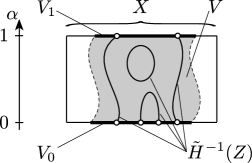
Figure 11: Intuition behind the proof of Lemma 27. The rectangle represents $[0,1]\times X$, the gray area is $V$ and the curves contained in it are $\widetilde{H}^{-1}(Z)$. An important feature is that these curves cannot pass through $\partial V$, which is represented by the dotted lines.

Lemma 27.

If $H:\left[0,1\right]\times\overline{X}\rightarrow Y$ is continuous, $H\left(\partial V\right)\cap\overline{Z}=\emptyset$ and $H\left(\overline{V}\right)\cap\partial Z=\emptyset$ then

$$I_{2}\left(H\left(0,\cdot\right),V_{0},Z\right)=I_{2}\left(H\left(1,\cdot\right),V_{1},Z\right).$$

Proof.

The proof follows from mirror arguments to the proof of the homotopy property of the intersection number (see Lemma 29 in A). The intuition behind the proof is given in Figure 11.

By performing an arbitrarily small modification of $H$ we can obtain $\widetilde{H}$ for which $\widetilde{H}\left(0,\cdot\right)$ and $\widetilde{H}\left(1,\cdot\right)$ are transversal to $Z$ and that $\widetilde{H}|_{V}$ is smooth and transversal to $Z$. We can make the modification small enough so that for $\beta\in\left[0,1\right]$,

$$\left(\left(1-\beta\right)H+\beta\widetilde{H}\right)\left(\partial V\right)\cap\overline{Z} =\emptyset,$$

$$\left(\left(1-\beta\right)H+\beta\widetilde{H}\right)\left(\overline{V}\right)\cap\partial Z =\emptyset.$$

This in particular implies that for $d=0,1$, $H\left(d,\cdot\right)$ and $\widetilde{H}\left(d,\cdot\right)$ are homotopic through an admissible homotopy, so

$$I_{2}\left(H\left(d,\cdot\right),V_{d},Z\right)=I_{2}\left(\widetilde{H}\left(d,\cdot\right),V_{d},Z\right)\qquad\mathchoice{\hbox{{for }}}{\hbox{{\firstchoice@false for }}}{\hbox{{\firstchoice@false for }}}{\hbox{{\firstchoice@false for }}}d=0,1.$$ (51)

Since $\widetilde{H}|_{V}$ is transversal to $Z$, we have that $\widetilde{H}^{-1}\left(Z\right)$ is a $1$-dimensional submanifold with boundary of $V$, the boundary being (see Figure 11)

$$\partial\widetilde{H}^{-1}(Z)=\{0\}\times\widetilde{H}\left(0,\cdot\right)^{-1}(Z)\,\cup\,\{1\}\times\widetilde{H}\left(1,\cdot\right)^{-1}(Z).$$

By the classification of $1$-manifolds [GP74], $\partial\widetilde{H}^{-1}(Z)$ consists of an even number of points, hence

$$\#\widetilde{H}\left(0,\cdot\right)^{-1}(Z)\equiv\#\widetilde{H}\left(1,\cdot\right)^{-1}(Z)\,\mathrm{mod}\,2.$$

This by the intersection property for transversal maps means that

$$I_{2}\left(\widetilde{H}\left(0,\cdot\right),V_{0},Z\right)=I_{2}\left(\widetilde{H}\left(1,\cdot\right),V_{1},Z\right),$$

which combined with (51) concludes our proof. ∎

The proof of Theorem 15 is based on the classical ideas that stem from the Leray-Schauder continuation theorem [Leray]. This is a standard technique (see [Mawhin] for an overview of related results). We adopt it to be combined with the intersection number in our particular setting.

Proof of Theorem 15.

Let us fix $\theta=\Theta_{0}$. We will look for a connected component $C$ in the set $\left[0,1\right]\times E_{\Theta_{0}}$. In fact it will turn out that we can find $C$ in $\left[0,1\right]\times\left(E_{\Theta_{0}}^{u}\oplus\left\{0\right\}^{s}\right)$. Let $D_{\Theta_{0}}^{u}:=\left\{x\in E_{\Theta_{0}}^{u}|\,\left\|x\right\|_{u}\leq 1\right\}$. The set $D_{\Theta_{0}}^{u}$ is a compact metric space, with the metric defined by the norm on the bundle $E_{\Theta_{0}}^{u}$. Let us equip $\left[0,1\right]\times D_{\Theta_{0}}^{u}$ with a metric

$$m\left(\left(\alpha_{1},x_{1}\right),\left(\alpha_{2},x_{2}\right)\right):=\max\{\left|\alpha_{1}-\alpha_{2}\right|,\left\|x_{1}-x_{2}\right\|_{u}\},$$ (52)

and define a set

$$K:=\left\{\left(\alpha,x\right)|\;x\in D_{\Theta_{0}}^{u},\ f_{\alpha}^{i}\left(\Theta_{0};x,0\right)\in D\mathchoice{\hbox{{ for all }}}{\hbox{{\firstchoice@false for all }}}{\hbox{{\firstchoice@false for all }}}{\hbox{{\firstchoice@false for all }}}i\in\mathbb{N}\mathchoice{\hbox{{ and }}}{\hbox{{\firstchoice@false and }}}{\hbox{{\firstchoice@false and }}}{\hbox{{\firstchoice@false and }}}\alpha\in[0,1]\right\}.$$

From the covering $D_{\Theta_{0}}\binrel@{\Longrightarrow}\binrel@@{\mathop{\kern 0.0pt\Longrightarrow}\limits^{f_{\alpha}}}D$ it follows that any point from $D_{\Theta_{0}}^{-}$ exits $D$, which implies

$$K\cap\left(\left[0,1\right]\times\partial D_{\Theta_{0}}^{u}\right)=\emptyset.$$ (53)

Since the family $f_{\alpha}$ is continuous and $D$ is closed, if we take a convergent sequence $(\alpha_{j},x_{j})\in K,$ then $\lim_{j\rightarrow\infty}f_{\alpha_{j}}^{i}\left(\Theta_{0};x_{j},0\right)\in D$, so $K$ is a compact metric space with the metric (52). Let $L_{\alpha},L_{\alpha}^{k}\subset D_{\Theta_{0}}^{u}$ be compact sets defined as

$$L_{\alpha}:=\left\{x\in D_{\Theta_{0}}^{u}|\;f_{\alpha}^{i}\left(\Theta_{0};x,0\right)\in D\mathchoice{\hbox{{ for all }}}{\hbox{{\firstchoice@false for all }}}{\hbox{{\firstchoice@false for all }}}{\hbox{{\firstchoice@false for all }}}i\in\mathbb{N}\right\},$$

$$L_{\alpha}^{k}:=\left\{x\in D_{\Theta_{0}}^{u}|\;f_{\alpha}^{i}\left(\Theta_{0};x,0\right)\in D\mathchoice{\hbox{{ for }}}{\hbox{{\firstchoice@false for }}}{\hbox{{\firstchoice@false for }}}{\hbox{{\firstchoice@false for }}}i=0,\ldots,k\right\},$$

for $\alpha\in\left[0,1\right]$ and $k\in\mathbb{N}$. Note that $L_{\alpha}\subset L_{\alpha}^{k}$ and $L_{\alpha}^{k+1}\subset L_{\alpha}^{k}$ for $\alpha\in\left[0,1\right]$ and $k\in\mathbb{N}.$

Let $K_{0}:=\left\{0\right\}\times L_{0}$ and $K_{1}:=\left\{1\right\}\times L_{1}$. By Theorem 8, $K_{0}$ and $K_{1}$ are nonempty. (Here we in fact used the fact that in the proof we have established that we can take the $v$ from the statement of Theorem 8 to be from $E_{\Theta_{0}}^{u}\oplus\left\{0\right\}^{s}\cap D$.) By Lemma 26 we have two possibilities. The first ensures our claim, so we need to rule out the second one, which will conclude our proof.

Suppose that we have two disjoint compact sets $\widehat{K_{0}}$ and $\widehat{K_{1}}$ such that $K=\widehat{K_{0}}\cup\widehat{K_{1}}$ and $K_{i}\subset\widehat{K_{i}}$ for $i=0,1$. Let us take small $\varepsilon$ so that

$$\varepsilon<\frac{1}{2}\mathrm{dist}\left(\widehat{K_{0}},\widehat{K_{1}}\right).$$ (54)

Because of (53), we can take $\varepsilon>0$ small enough so that in addition to (54) we have

$$U:=\left\{\left(\alpha,x\right)\in\left[0,1\right]\times D_{\Theta_{0}}^{u}|\;\mathrm{dist}\left(\left(\alpha,x\right),\widehat{K_{0}}\right)<\varepsilon\right\}\subset\left[0,1\right]\times\mathrm{int}D_{\Theta_{0}}^{u}.$$

Clearly $K_{0}\subset U$ and also by (54) we see that $K_{1}\cap U=\emptyset$. We shall use the notation $U_{\alpha}=\left\{x|\,\left(\alpha,x\right)\in U\right\}$, so we can rewrite the previous statement as $L_{0}\subset U_{0}$ and $L_{1}\cap U_{1}=\emptyset$. Since

$$L_{\alpha}=\bigcap_{k=0}^{\infty}L_{\alpha}^{k}\qquad\mathchoice{\hbox{{for }}}{\hbox{{\firstchoice@false for }}}{\hbox{{\firstchoice@false for }}}{\hbox{{\firstchoice@false for }}}\alpha\in\left[0,1\right],$$

by taking sufficiently large $k$ we will have

$$L_{0}^{k} \subset U_{0},$$ (55)

$$L_{1}^{k}\cap U_{1} =\emptyset,$$ (56)

and since $\partial U\cap K=\emptyset,$ we can also choose $k$ large enough so that

$$L_{\alpha}^{k}\cap\partial U_{\alpha}=\emptyset\qquad\mathchoice{\hbox{{for }}}{\hbox{{\firstchoice@false for }}}{\hbox{{\firstchoice@false for }}}{\hbox{{\firstchoice@false for }}}\alpha\in\left[0,1\right].$$ (57)

Consider $Y$ and $Z$ defined in (21–22), and take

$$\overline{V}:=\overline{U}\times\binrel@{\underbrace{\mathbf{D}\times\ldots\times\mathbf{D}}}\binrel@@{\mathop{\kern 0.0pt\underbrace{\mathbf{D}\times\ldots\times\mathbf{D}}}\limits_{k}}.$$ (58)

We shall consider $H=\left(H_{1},\ldots,H_{k},H_{k+1}\right):\overline{V}\rightarrow Y$ which is defined for points

$$\mathbf{x}=\left(\left(\Theta_{0};x_{0}\right),\left(\theta_{1};x_{1},y_{1},z_{1}\right),\ldots,\left(\theta_{k};x_{k},y_{k},z_{k}\right)\right)\in\overline{V}_{\alpha}$$

as

$$H_{1}\left(\alpha,\mathbf{x}\right) :=\left(f_{\alpha}\left(\Theta_{0};x_{0},0\right),0\right)-\left(\theta_{1};x_{1},y_{1},z_{1}\right),$$

$$H_{2}\left(\alpha,\mathbf{x}\right) :=\left(f_{\alpha}\left(\theta_{1};x_{1},y_{1}\right),0\right)-\left(\theta_{2};x_{2},y_{2},z_{2}\right),$$

$$\;\;\;\vdots$$

$$H_{k}\left(\alpha,\mathbf{x}\right) :=\left(f_{\alpha}\left(\theta_{k-1};x_{k-1},y_{k-1}\right),0\right)-\left(\theta_{k};x_{k},y_{k},z_{k}\right),$$

$$H_{k+1}\left(\alpha,\mathbf{x}\right) :=f_{\alpha}\left(\theta_{k};x_{k},y_{k}\right).$$

We will now show that

$$H\left(\partial V\right)\cap\overline{Z}=\emptyset.$$ (59)

This follows from mirror arguments to those used to show (28). The only difference is that we also need to consider the case when $\left(\alpha,\mathbf{x}\right)\in V$ is such that $\left(\alpha,x_{0}\right)\in\partial U$. In such case, due to (57), we see that we can not have $f_{\alpha}^{k}\left(\Theta_{0};x_{0},0\right)\in D$ so any point for which $H\left(\alpha,\mathbf{x}\right)\in Z$ can not have $\left(\alpha,x_{0}\right)\in\partial U$. We have thus shown (59).

From arguments identical to showing (29) we also obtain

$$H\left(\overline{V}\right)\cap\partial Z=\emptyset.$$ (60)

By Lemma (27) together with (59–60) we obtain

$$I_{2}\left(H\left(0,\cdot\right),V_{0},Z\right)=I_{2}\left(H\left(1,\cdot\right),V_{1},Z\right).$$ (61)

We will now compute $I_{2}\left(H\left(0,\cdot\right),V_{0},Z\right)$. Let $\overline{X}$ be the set defined in (20). The first coordinate of $V_{0}$ is $U_{0}$ (see (58)). By (55) $U_{0}$ contains all points $x_{0}$ such that $f_{0}^{i}\left(\Theta_{0};x_{0},0\right)\in D$ for every $i\in\left\{1,\ldots,k\right\}.$ This means that if $\mathbf{x}\in X\setminus V_{0}$ then we can not have $f_{0}^{i}\left(\Theta_{0};x_{0},0\right)\in D$ for any $i\in\left\{1,\ldots,k\right\}$. Thus, for $\mathbf{x}\in X\setminus V_{0}$ we can not have $H\left(0,\mathbf{x}\right)\in Z$, hence

$$H\left(0,X\right)\cap Z=H\left(0,V_{0}\right)\cap Z.$$

Note that from (59) $H\left(0,\partial V_{0}\right)\cap\overline{Z}=\emptyset$, so from the excision property

$$I_{2}\left(H\left(0,\cdot\right),X,Z\right)=I_{2}\left(H\left(0,\cdot\right),V_{0},Z\right).$$ (62)

In the proof of Theorem 8 we have established that $I_{2}\left(H\left(0,\cdot\right),X,Z\right)=1,$ so by (62)

$$I_{2}\left(H\left(0,\cdot\right),V_{0},Z\right)=1.$$ (63)

We will now compute $I_{2}\left(H\left(1,\cdot\right),V_{1},Z\right)$. The set $L_{1}^{k}$ contains all points $x_{0}$ for which $f_{1}^{i}\left(\Theta_{0};x_{0},0\right)\in D$ for all $i\in\left\{1,\ldots,k\right\}$. If $\mathbf{x}\in V_{1}$, then $x_{0}\in U_{1}$, so by (56) we can not have $f_{1}^{i}\left(\Theta_{0};x_{0},0\right)\in D$ for all $i\in\left\{1,\ldots,k\right\}$. This means that for $\mathbf{x}\in V_{1}$, $H\left(1,\mathbf{x}\right)\notin Z$, so by the intersection property

$$I_{2}\left(H\left(1,\cdot\right),V_{1},Z\right)=0.$$ (64)

By (61), (63), (64) we have obtained a contradiction. This means that we have ruled out the second case of Lemma 26 and finished our proof. ∎

9 Proof of Theorem 16

Proof.

The proof follows along the same lines as the proof of Theorem 15.

Let us fix $\theta=\Theta_{0}$. We will look for a connected component $C$ in $\left[0,1\right]\times E_{\Theta_{0}}$. The set $D_{\Theta_{0}}$ is a compact metric space, with the metric defined by the norm on the bundle $E_{\Theta_{0}}$. We equip $\left[0,1\right]\times D_{\Theta_{0}}$ with a metric

$$m\left(\left(\alpha_{1},v_{1}\right),\left(\alpha_{2},v_{2}\right)\right)=\max\{\left|\alpha_{1}-\alpha_{2}\right|,\left\|v_{1}-v_{2}\right\|\},$$ (65)

and define a set

$$K :=\{\left(\alpha,v\right)|\;v\in D_{\Theta_{0}}\mathchoice{\hbox{{ and there exists a trajectory of }}}{\hbox{{\firstchoice@false and there exists a trajectory of }}}{\hbox{{\firstchoice@false and there exists a trajectory of }}}{\hbox{{\firstchoice@false and there exists a trajectory of }}}f_{\alpha}\mathchoice{\hbox{{ in }}}{\hbox{{\firstchoice@false in }}}{\hbox{{\firstchoice@false in }}}{\hbox{{\firstchoice@false in }}}D$$

$$\qquad\mathchoice{\hbox{{ passing through }}}{\hbox{{\firstchoice@false passing through }}}{\hbox{{\firstchoice@false passing through }}}{\hbox{{\firstchoice@false passing through }}}v\}.$$

We shall say that a sequence $\left\{v_{i}\right\}$ is a trajectory of $f_{\alpha}$ of length $k$ in $D$ passing through $v$ if $v_{0}=v$, $v_{i}\in D$ for $i=-k,\ldots,k$ and $f_{\alpha}\left(v_{i}\right)=v_{i+1}$ for $i=-k,\ldots,k-1$.

The set $K$ is a compact metric space with the metric (65). For $\alpha\in\left[0,1\right]$ and $k\in\mathbb{N}$ let $L_{\alpha},L_{\alpha}^{k}\subset D_{\Theta_{0}}^{u}$ be compact sets defined as

$$L_{\alpha} :=\left\{v\in D_{\Theta_{0}}|\;\mathchoice{\hbox{{there exists a trajectory of }}}{\hbox{{\firstchoice@false there exists a trajectory of }}}{\hbox{{\firstchoice@false there exists a trajectory of }}}{\hbox{{\firstchoice@false there exists a trajectory of }}}f_{\alpha}\mathchoice{\hbox{{ in }}}{\hbox{{\firstchoice@false in }}}{\hbox{{\firstchoice@false in }}}{\hbox{{\firstchoice@false in }}}D\mathchoice{\hbox{{ passing through }}}{\hbox{{\firstchoice@false passing through }}}{\hbox{{\firstchoice@false passing through }}}{\hbox{{\firstchoice@false passing through }}}v\right\},$$

$$L_{\alpha}^{k} :=\{v\in D_{\Theta_{0}}|\;\mathchoice{\hbox{{there exists a trajectory of }}}{\hbox{{\firstchoice@false there exists a trajectory of }}}{\hbox{{\firstchoice@false there exists a trajectory of }}}{\hbox{{\firstchoice@false there exists a trajectory of }}}f_{\alpha}\mathchoice{\hbox{{ of length }}}{\hbox{{\firstchoice@false of length }}}{\hbox{{\firstchoice@false of length }}}{\hbox{{\firstchoice@false of length }}}k\mathchoice{\hbox{{ in }}}{\hbox{{\firstchoice@false in }}}{\hbox{{\firstchoice@false in }}}{\hbox{{\firstchoice@false in }}}D$$

$$\qquad\mathchoice{\hbox{{ passing through }}}{\hbox{{\firstchoice@false passing through }}}{\hbox{{\firstchoice@false passing through }}}{\hbox{{\firstchoice@false passing through }}}v\}.$$

Note that $L_{\alpha}^{k+1}\subset L_{\alpha}^{k}$ and $L_{\alpha}\subset L_{\alpha}^{k}$ for $\alpha\in\left[0,1\right]$ and $k\in\mathbb{N}.$

Let $K_{0}:=\left\{0\right\}\times L_{0}$ and $K_{1}:=\left\{1\right\}\times L_{1}$. By Theorem 13, $K_{0}$ and $K_{1}$ are nonempty. By Lemma 26 we have two possibilities. The first ensures our claim, so we need to rule out the second one, which will conclude our proof.

Suppose that we have disjoint compact $\widehat{K_{0}},$ $\widehat{K_{1}}$ such that $K=\widehat{K_{0}}\cup\widehat{K_{1}}$ and $K_{0}\subset\widehat{K_{0}}$, $K_{1}\subset\widehat{K_{1}}$. Consider $\varepsilon<\frac{1}{2}\mathrm{dist}\left(\widehat{K_{0}},\widehat{K_{1}}\right)$, chosen sufficiently small so that

$$U:=\left\{\left(\alpha,v\right)\in\left[0,1\right]\times D_{\Theta_{0}}|\;\mathrm{dist}\left(\left(\alpha,v\right),\widehat{K_{0}}\right)<\varepsilon\right\}\subset\left[0,1\right]\times\mathrm{int}D_{\Theta_{0}}.$$

We shall embed $U$ in $\mathbb{R}^{2n}$ (we use Notation 23)

$$\mathbf{U:}=\left\{\left(\alpha,\left(v,z\right)\right)\in\left[0,1\right]\times\mathcal{T}\,|\;\left(\alpha,v\right)\in U,\ \left\|z\right\|_{\mathbb{R}^{2n}}\leq\delta\right\}\subset\mathbb{R}^{2n}.$$

Consider $Y$ and $Z$ defined in (47–48), and take

$$\overline{V}:=D^{u}\times\binrel@{\underbrace{\mathbf{D}\times\ldots\times\mathbf{D}}}\binrel@@{\mathop{\kern 0.0pt\underbrace{\mathbf{D}\times\ldots\times\mathbf{D}}}\limits_{k}}\times\overline{\mathbf{U}}\times\binrel@{\underbrace{\mathbf{D}\times\ldots\times\mathbf{D}}}\binrel@@{\mathop{\kern 0.0pt\underbrace{\mathbf{D}\times\ldots\times\mathbf{D}}}\limits_{k}}.$$

We shall consider $H=\left(H_{-k},\ldots,H_{k},H_{k+1}\right):\overline{V}\rightarrow Y$ which is defined for points

$$\mathbf{x} =(\left(\theta_{-k-1};x_{-k-1}\right),\left(\theta_{-k};x_{-k},y_{-k},z_{-k}\right),\ldots,\left(\theta_{-1};x_{-1},y_{-1},z_{-1}\right),$$

$$\qquad\qquad\qquad\left(\Theta_{0};x_{0},y_{0},z_{0}\right),\left(\theta_{1};x_{1},y_{1},z_{1}\right),\ldots,\left(\theta_{k};x_{k},y_{k},z_{k}\right))$$

as (compare with (49) used in the proof of Theorem 13)

$$H_{-k}\left(\alpha,\mathbf{x}\right) :=\left(f_{\alpha}\left(\theta_{-k-1};x_{-k-1},0\right),0\right)-\left(\theta_{-k};x_{-k},y_{-k},z_{-k}\right),$$

$$H_{-k+1}\left(\alpha,\mathbf{x}\right) :=\left(f_{\alpha}\left(\theta_{-k};x_{-k},y_{-k}\right),0\right)-\left(\theta_{-k+1};x_{-k+1},y_{-k+1},z_{-k+1}\right),$$

$$\;\;\;\vdots$$

$$H_{-1}\left(\alpha,\mathbf{x}\right) :=\left(f_{\alpha}\left(\theta_{-2};x_{-2},y_{-2}\right),0\right)-\left(\theta_{-1};x_{-1},y_{-1},z_{-1}\right),$$

$$H_{0}\left(\alpha,\mathbf{x}\right) :=\left(f_{\alpha}\left(\theta_{-1};x_{-1},y_{-1}\right),0\right)-\left(\Theta_{0};x_{0},y_{0},z_{0}\right),$$

$$H_{1}\left(\alpha,\mathbf{x}\right) :=\left(f_{\alpha}\left(\Theta_{0};x_{0},y_{0}\right),0\right)-\left(\theta_{1};x_{1},y_{1},z_{1}\right),$$

$$H_{2}\left(\alpha,\mathbf{x}\right) :=\left(f_{\alpha}\left(\theta_{1};x_{1},y_{1}\right),0\right)-\left(\theta_{2};x_{2},y_{2},z_{2}\right),$$

$$\;\;\;\vdots$$

$$H_{k}\left(\alpha,\mathbf{x}\right) :=\left(f_{\alpha}\left(\theta_{k-1};x_{k-1},y_{k-1}\right),0\right)-\left(\theta_{k};x_{k},y_{k},z_{k}\right),$$

$$H_{k+1}\left(\alpha,\mathbf{x}\right) :=f_{\alpha}\left(\theta_{k};x_{k},y_{k}\right).$$

From now on we skip the details since they follow along the same lines as in the proof of Theorem 15. We just outline the steps: Using Lemma 27 we can show that

$$I_{2}\left(H\left(0,\cdot\right),V_{0},Z\right)=I_{2}\left(H\left(1,\cdot\right),V_{1},Z\right).$$ (66)

Using the excision property, for $X$ defined in (46), we obtain

$$I_{2}\left(H\left(0,\cdot\right),V_{0},Z\right)=I_{2}\left(H\left(0,\cdot\right),X,Z\right)=1.$$ (67)

From the fact that $V_{1}$ can not contain trajectories of length $k$ in $D$ passing through $D_{\Theta_{0}}$ we also obtain

$$I_{2}\left(H\left(1,\cdot\right),V_{1},Z\right)=0.$$ (68)

Conditions (66–68) lead to a contradiction, which concludes our proof. ∎

10 Proof of Lemma 20.

Proof.

Let $E=E^{u}\oplus E^{s}$ and consider $l:E\rightarrow E$ defined as

$$l\left(\theta;x,y\right):=\left(f\left(\theta\right);df(\theta)x,df(\theta)y\right).$$

Note $l$ is well defined since the splitting (6) is invariant under the action of the differential $df$. We shall refer to $l$ as the ‘linearized map’. Note that

$$l^{k}\left(\theta;x,y\right)=\left(f^{k}\left(\theta\right);df^{k}(\theta)x,df^{k}(\theta)y\right).$$

For $r>0$ we define $D(r)\subset E$ as

$$D(r):=\left\{\left(\theta;x,y\right)|\;\theta\in\Lambda,\ x\in E_{\theta}^{u},\ y\in E_{\theta}^{s},\ \left\|x\right\|\leq r,\ \left\|y\right\|\leq r\right\}.$$

We will show that for any $r>0$ we have

$$D(r)\binrel@{\Longrightarrow}\binrel@@{\mathop{\kern 0.0pt\Longrightarrow}\limits^{l^{k}}}D(r).$$ (69)

The homotopy $h$ (see Definition 9) for the covering (69) can be taken as

$$h\left(\beta,\left(\theta;x,y\right)\right):=\left(f^{k}\left(\theta\right);df^{k}(\theta)x,(1-\beta)df^{k}(\theta)y\right),\quad\beta\in\left[0,1\right].$$ (70)

Before showing that $h$ satisfies all required conditions we note that since $\lambda<1$, from $k>\log_{\lambda}\frac{1}{C}$ it follows that $C\lambda^{k}<1$. Using (7) we also see that for any $\theta\in\Lambda$ and $x\in E_{\theta}^{u}$

$$\left\|x\right\|=\left\|d\left(f^{-k}\circ f^{k}\right)(\theta)x\right\|=\left\|df^{-k}(f^{k}(\theta))df^{k}(\theta)x\right\|\leq C\lambda^{k}\left\|df^{k}(\theta)x\right\|.$$ (71)

We will now show that $h$ satisfies conditions from Definition 9. If $\left(\theta;x,y\right)\in D^{-}\left(r\right)$, meaning that $\left\|x\right\|=r,$ then by (71), $\left\|df^{k}(\theta)x\right\|>\left(C\lambda^{k}\right)^{-1}\left\|x\right\|>r$, hence $h\left(\beta,\left(\theta;x,y\right)\right)\notin D(r)$, ensuring (2).

For any $\left(\theta;x,y\right)\in D\left(r\right)$, by (8), $\left\|\left(1-\beta\right)df^{k}\left(\theta\right)y\right\|<C\lambda^{k}\left\|y\right\|<r$, so $h\left(\beta,\left(\theta;x,y\right)\right)\notin D^{+}\left(r\right)$, which means that we have verified (3).

From (70) we see that the map $\eta$ from Definition 9 is $\eta=\left(f|_{\Lambda}\right)^{k}$. Since $\Lambda$ is invarant under $f,$ and $f$ is a diffeomorphism, $\left(f|_{\Lambda}\right)^{k}$ is also a diffeomorphism, so $\deg_{2}\left(\eta\right)=1$ ensuring (4). Also from (70), $A_{\theta}=df^{k}(\theta)|_{E_{\theta}^{u}}$. Since $C\lambda^{k}<1$, by (71) $A_{\theta}$ is expanding. We have thus established (69).

For sufficiently small $r$ the linearized dynamics inside $D\left(r\right)$ is topologically conjugate to the true dynamics in a neighborhood of $\Lambda$, i.e. $l^{k}\circ g=g\circ f^{k}$ where $g$ is the conjugating homeomorphism [Pugh1970]. The set $D=g^{-1}\left(D(r)\right)$, equipped with the structure of the vector bundle $E$ induced by $g$, constitutes the neighbourhood of $\Lambda$ in $M$ which $f^{k}$-covers itself. ∎

11 Acknowledgements

We would like to thank Rafael de la Llave for his encouragement and suggestions. In particular, we thank him for pointing us to the Leray-Schauder continuation techniques and for his suggestions that led us to formulating Theorems 15 and 16. We would also like to thank the anonymous Reviewers for their comments, suggestions and corrections, which helped us improve our paper.

Appendix A Construction of the intersection number

Here we present a brief overview of the construction of $I_{2}\left(f,X,Z\right)$.

Lemma 28.

If $f$ is admissible, $f|_{X}$ is smooth and transversal to $Z$, then the number $\#f^{-1}\left(Z\right)$ is finite.

Proof.

Since $f$ is admissible, $f^{-1}(Z)\$ is separated from $\partial X$ and $f^{-1}\left(\partial Z\right)=\emptyset$. From the transversality of $f|_{X}$ to $Z$ we obtain that $f^{-1}(Z)$ is a $0$-dimensional submanifold of $X$. From transversality, the points in $f^{-1}(Z)$ cannot accumulate, and since they are contained in the compact set $\overline{X}$, their number is finite. ∎

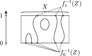
Figure 12: Intuition behind the proof of Lemma 29. The rectangle represents $[0,1]\times X$ and the curves contained in it are $H^{-1}(Z)$. An important feature is that due to the admissibility of the homotopy these curves cannot pass through $[0,1]\times\partial X$, which is represented by the dotted lines.

Above we have shown that for $f|_{X}$ transversal to $Z$ defining the intersection number as

$$I_{2}\left(f,X,Z\right):=\#f^{-1}\left(Z\right)\,\mathrm{mod}\,2$$ (72)

makes sense since we do not have infinity on the right hand side of the defining equation. We now show that this number remains constant when passing through an admissible homotopy. The proof of the following lemma is based on the fact that if we have a homotopy $H$ between two smooth maps, both being transversal to some given manifold, then we can make $H$ transversal to that manifold by an arbitrarily small modification (see [GP74, Extension Theorem and Corollary that follows] for details).

Lemma 29.

Assume that $f_{0},f_{1}:\overline{X}\rightarrow Y$ are two admissible maps and that $f_{0}|_{X}$ and $f_{1}|_{X}$ are smooth and transversal to $Z$. If $f_{0}$ and $f_{1}$ are homotopic via an admissible homotopy, then

$$\#f_{0}^{-1}(Z)=\#f_{1}^{-1}(Z)\,\mathrm{mod\,}2.$$

Proof.

The intuition behind the proof is given in Figure 12.

Let $F:[0,1]\times\overline{X}\rightarrow Y$ be an admissible homotopy from $f_{0}$ to $f_{1}$. By performing an arbitrarily small modification we can arrive at an admissible $F$ such that $F|_{[0,1]\times X}$ is smooth and transversal to $Z$. Note that since $F$ is admissible, $F^{-1}\left(Z\right)$ does not intersect $\left[0,1\right]\times\partial X$. Since $F|_{[0,1]\times X}$ is transversal to $Z$, we have that $F^{-1}\left(Z\right)$ is a $1$-dimensional submanifold with boundary of $[0,1]\times X$, the boundary being

$$\partial F^{-1}(Z)=\{0\}\times f_{0}^{-1}(Z)\,\cup\,\{1\}\times f_{1}^{-1}(Z).$$

By the classification of $1$-manifolds [GP74], $\partial F^{-1}(Z)$ consists of an even number of points, hence

$$\#f_{0}^{-1}(Z)=\#f_{1}^{-1}(Z)\,\mathrm{mod}\,2,$$

as required. ∎

For any admissible map $f$ we can find an admissible map $g,$ arbitrarily close to $f$, for which $g|_{X}$ is smooth, and such that $f$ and $g$ are homotopic through an admissible homotopy. If $g|_{X}$ is not transversal to $Z$, then we can again perform an arbitrarily small modification to obtain transversality of $g|_{X}$ to $Z$ . We can therefore define

$$I_{2}\left(f,X,Z\right):=\#g^{-1}(Z)\,\mathrm{mod\,}2,$$ (73)

where $f$ and $g$ are as above. By Lemma 28 the number $\#g^{-1}(Z)$ is finite an by Lemma 29 the number $\#g^{-1}(Z)\,\mathrm{mod\,}2$ does not depend on the choice of $g$, so $I_{2}\left(f,X,Z\right)$ from (73) is well-defined.

What is left is to prove that for $I_{2}\left(f,X,Z\right)$ defined in (73) we have the homotopy property, intersection property and the excision property.

Lemma 30.

If $f_{1},f_{2}$ are homotopic through an admissible homotopy then $I_{2}(f_{1},X,Z)=I_{2}(f_{2},X,Z)$.

Proof.

Since $f_{1},f_{2}$ are homotopic through an admissible homotopy, they are admissible. As in the construction leading to (73) we can find two smooth admissible maps $g_{1}$ and $g_{2}$, homotopic through an admissible homotopy to $f_{1}$ and $f_{2}$, respectively, for which $g_{1}|_{X}$ and $g_{2}|_{X}$ are transversal to $Z$. Since $g_{1}$ and $g_{2}$ are homotopic through an admissible homotopy (which is a composition of admissible homotopies: $g_{1}$ to $f_{1}$, $f_{1}$ to $f_{2}$, and $f_{2}$ to $g_{2}$) from (73) and Lemma 29 we obtain

$$I_{2}(f_{1},X,Z)=\#g_{1}^{-1}(Z)\mbox{ mod }2=\#g_{2}^{-1}(Z)\mbox{ mod }2=I_{2}(f_{2},X,Z),$$

as required. ∎

Lemma 31.

Let $f$ be an admissible map. If $I_{2}\left(f,X,Z\right)\neq 0$ then $f\left(X\right)\cap Z$ is nonempty.

Proof.

We will show that if $f\left(X\right)\cap Z=\emptyset$ then $I_{2}\left(f,X,Z\right)=0$.

Assume that $f\left(X\right)\cap Z=\emptyset$. By admissibility $f(\partial X)\cap\overline{Z}=\emptyset$ and $f(\overline{X})\cap\partial Z=\emptyset$, so then $f(\overline{X})\cap\overline{Z}=\emptyset.$

We can approximate $f|_{X}$ by an arbitrarily close smooth map $g:X\rightarrow Y$, homotopic to $f|_{X}$. We can extend this $g$ to $\overline{X}$ in the natural way to obtain $g:\overline{X}\rightarrow Y$. We can take this $g$ close enough so that it is homotopic to $f$ by an admissible homotopy and $g(\overline{X})\cap\overline{Z}=\emptyset.$ Since the intersection of $g(X)$ with $Z$ is empty and $g|_{X}$ is smooth, it is transversal to $Z$ (an empty intersection is by definition transversal), and

$$I_{2}\left(f,X,Z\right)=I_{2}\left(g,X,Z\right)=\#g^{-1}\left(Z\right)\,\mathrm{mod}\,2=0,$$

as required. ∎

Lemma 32.

Let $f:X\rightarrow Y$ be an admissible map. If $V$ is an open subset of $X$ such that $f\left(X\right)\cap Z=f\left(V\right)\cap Z$, and $f\left(\partial V\right)\cap\overline{Z}=\emptyset$ then

$$I_{2}(f,X,Z)=I_{2}\left(f|_{\overline{V}},V,Z\right).$$

Proof.

We see that $f|_{\overline{V}}$ is admissible since

$$f\left(\overline{V}\right)\cap\partial Z\subset f\left(\overline{X}\right)\cap\partial Z=\emptyset.$$

We can find a $g$ arbitrarily close to $f$, homotopic through an admissible homotopy (admissible both for $X$ and $V$) so that $g|_{X}$ is smooth. If $g|_{X}$ is not transversal to $Z$, then we can make an arbitrarily small modification of $g|_{X}$ to make it transversal. We can take $g$ close enough to $f$ so that $g\left(X\right)\cap Z=g\left(V\right)\cap Z$. Since $g|_{X}$ is transversal to $Z$, $g|_{V}$ is also transversal to $Z$. From (72–73)

$$I_{2}(f,X,Z) =I_{2}(g,X,Z)=\#g^{-1}\left(Z\right)\,\mathrm{mod}\,2$$

$$\qquad\qquad=I_{2}\left(g|_{\overline{V}},V,Z\right)=I_{2}\left(f|_{\overline{V}},V,Z\right),$$

as required. ∎

Appendix B Code for the computer assisted proof

The program validates that $D\binrel@{\Longrightarrow}\binrel@@{\mathop{\kern 0.0pt\Longrightarrow}\limits^{f}}D$. We write out the code and follow with comments.

#include <iostream>#include "capd/capdlib.h"  using namespace std; using namespace capd;const interval mu=interval(1)/interval(10);interval part(interval x,int N, int k)     { return x.left()+k*(x.right()-x.left())/N+(x-x.left())/N; }interval hx(interval alpha,interval x,interval y)     { return alpha*2*x+(1-alpha)*(-8*x/5+4*power(x,3)+x*y/2); }interval hy(interval alpha,interval theta,interval x,interval y)     { return (1-alpha)*(mu*y+2*sin(theta)/5+x*cos(theta)); }bool ExitCondition(interval alpha,interval Bu,interval Bs)  {   if(not(hx(alpha,Bu.left() ,Bs)<Bu)) return 0;   if(not(hx(alpha,Bu.right(),Bs)>Bu)) return 0;   return 1;}bool EntryCondition(interval alpha,interval theta,interval Bu,interval Bs,int N)  {   for(int i=0;i<N;i++)   {      for(int j=0;j<N;j++)      {         interval x=hx(alpha,part(Bu,N,i),part(Bs,N,j));         interval y=hy(alpha,theta,part(Bu,N,i),part(Bs,N,j));         if(not(x<Bu))            if(not(x>Bu))               if(not(subsetInterior(y,Bs))) return 0;      }   }   return 1;}int main(){   interval alpha=interval(0.0,1.0);   interval Lambda=interval(2)*interval::pi()*interval(0.0,1.0);   interval Bu=interval(-1.0,1.0);   interval Bs=interval(-1.2,1.2);   for(int k=0;k<4;k++)   {      for(int i=0;i<100;i++)      {         if(ExitCondition(part(alpha,4,k),Bu,Bs)==0) return 0;           if(EntryCondition(part(alpha,4,k),part(Lambda,100,i),Bu,Bs,50)==0) return 0;      }   }   cout << "proof complete" << endl; return 1;  }

• The code is based on the CAPD library for C++. To download and install the library follow the instructions found at http://capd.ii.uj.edu.pl.

• This routine computes the k-th part out of N of the interval x. The indexing is k=0,...,N-1. For example, if x=$[$1.0,2.0$]$ then for N=4 the 0-th part is $[$1.0,1.25$]$ and the 3-rd part is $[$1.75,2.0$]$.

• These routines are used for the homotopy (4.2) along the $x,y$ coordinates. Condition (4) follows directly from (4.2) so we need to validate (2–3), for which local projections onto $x,y$ are sufficient.

• We check that $h({\tt alpha}\times D^{-})\cap D=\emptyset$ and return 1 if this is validated and 0 otherwise. This function will later be used to check (2).

• This function is used to validate that $h({\tt alpha}\times D_{\tt theta})\cap D^{+}=\emptyset$. This is later used to validate (3). The test is performed by subdividing $D_{\tt theta}$ into $N^{2}$ cubes and checking that the image of each of them does not intersect $D^{+}$.

• This is the core of the program, where we validate (2–3). We do so by subdividing the parameter interval $[0,1]$ into four fragments and subdividing $\Lambda$ into $100$ parts.

• Once the program reaches this point we are sure that all the needed conditions are validated. The program takes a fraction of a second, running on a standard laptop.