Optimized Configuration Interaction Approach for Trapped Multiparticle Systems Interacting Via Contact Forces

Abstract

For one-dimensional systems with delta-contact interactions, the convergence of the exact-diagonalization method is tested with a basis of harmonic oscillator eigenfunctions with frequency $\Omega$ optimized through the minimization of the eigenenergy of the desired level. It is shown that within the framework of this approach the well-converged results can be achieved at much smaller dimensions of the Hamiltonian matrix than with the standard approach that uses $\Omega=1$. We present calculations for model systems of identical bosons with harmonic and double-well potentials. Our results show promising potential for diminishing the computational cost of numerical simulations of various systems of trapped ultracold atoms.

1 Introduction

Over the past two decades, there has been an explosion of interest in the properties of one-dimensional (1D) quantum gases with short-range interactions modelled by a Dirac $\delta$-potential. With the emergence of new technologies and experimental techniques, the properties of these systems, such as the number of particles, their interactions-, and the shape of the trapping potentials, can be controlled with high accuracy [1, 2]. As a result, it has become possible to simulate various physical phenomena in controllable ways that can even provide the opportunity to realize experimentally different toy models. Various physical realizations of systems of cold atoms are nowadays achieved [1, 2, 3, 4, 5, 6, 7]. In view of this tremendous technological progress, research activity has exploded in the area of investigating the many-body properties of various quantum composite cold-atom systems [8, 9, 10, 11, 12, 13, 14, 15, 16, 17, 18].

There are few 1D systems with contact interactions that can be solved analytically. The best known of these is the system composed of two identical particles held together in a harmonic trap, which has closed-form solutions in the whole interacting regime [19]. The Bethe ansatz method is known to be a solution for the 1D Bose gas in the absence of an external potential; that is, the so-called Lieb-Liniger model [20]. The most important result regarding the 1D gas is the famous Bose-Fermi mapping theorem [21] that maps the Tonks-Girardeau (TG) gas of bosons with infinitely strong repulsions to a free-fermion gas, which does not depend on the external potential. As a result, the theoretical study of TG gases is a relatively easy task even in the limit of large particle numbers. The first observation of TG gases in experiments [22] provided theoretical communities with the impetus to study the properties of TG gases under different external potentials [23, 24, 25, 26]. The Bose-Fermi mapping theorem also provides a tool for studying properties of multicomponent mixtures of strongly interacting gases [27, 28, 29, 30]. It is worth pointing out that a powerful pair-correlated variational approach to studying the ground states of bosonic systems with a harmonic trap has been developed in [31] and subsequently extended to fermionic mixtures [32] and to bosonic systems with different interactions between the pairs of atoms [33]. This approach can also be extended to other mixtures of cold atoms, such as boson-fermion mixtures [27] and bosonic mixtures [34].

However, in most cases, full numerical calculations are required to describe the transition between the weakly and strongly correlated regimes, and this is generally a cumbersome task. Numerical simulations of ultra-cold gases are often performed with the exact-diagonalization (ED) method and in the framework of the multiconfiguration time-dependent Hartree method [35] that has been extended for bosons [36] and fermions [37], as well as for bosonic (fermionic) mixtures [38, 39].

The standard ED method is based on the Rayleigh-Ritz procedure and uses as a variational wave function a finite linear combination of many-particle states of a proper symmetry under the exchange of particles, usually made up of solutions of the corresponding one-particle system. In contrast to variational methods that use single-trial wave functions, which are usually specialized to treat only ground states of specific systems, the ED method enables precise determination of ground- and higher bound-states in a systematic way.

In particular, most of the studies available in the literature about 1D systems with harmonic trapping potentials $x^{2}/2$ use the ED method with harmonic oscillator (HO) eigenfunctions:

$$u_{n}(x)=\left({\sqrt{\Omega}\over\sqrt{\pi}2^{n}n!}\right)^{{1\over 2}}\mathrm{e}^{-{\Omega x^{2}\over 2}}\mathbf{H}_{n}\left(\sqrt{\Omega}x\right),$$ (1)

with $\Omega=1$, where $\mathbf{H}_{n}$ is the $n$th order Hermite polynomial. However, this results in very poor convergence of the many-body eigenstates as a function of the number of basis states [40]. In fact, even for systems with small particle numbers, huge numbers of many-particle functions are needed to describe strongly interacting regime [13].

In this paper we show that the ED method with basis functions given by (1) can be a very effective tool for studying various trapped systems with delta interactions, provided the parameter $\Omega$ is variationally optimized. The structure of this paper is as follows. Section 2 outlines the formalism of the optimized ED (OED) approach. Section 3 tests the convergence of the OED method for the examples of harmonic and double-well potentials. Specifically, a significant improvement in the convergence is demonstrated for the harmonic trapping potential compared to the case without optimization of $\Omega$ ($\Omega=1$). Finally, section 4 presents some concluding remarks.

2 Optimized ED Approach

Without loss of generality, we deal only with systems of identical bosons. We begin with the dimensionless Hamiltonian to deal with any confining potential:

$$\hat{{\cal H}}=\sum_{i=1}^{N}h_{0}(x_{i})+g\sum_{i<j}\delta(x_{i}-x_{j}),$$ (2)

where the strength of the interaction is governed by the coefficient $g$ and $h_{0}$ is the one-body Hamiltonian given by

$$h_{0}(x)=-\frac{1}{2}\frac{\partial^{2}}{\partial x^{2}}+{V}(x).$$ (3)

The true $N$-particle bosonic wave function can be represented as a linear combination:

$$|\Psi\rangle=\sum_{\beta}a_{\beta}|\textbf{u}_{\beta}\rangle.$$ (4)

Here, $|\textbf{u}_{\beta}\rangle$ denotes the permanents that are constructed from the one-particle basis (1), which in the occupation-number representation take the form

$$|\mathbf{u}_{\beta}\rangle=|n_{0},n_{1},...\rangle_{\Omega}.$$ (5)

This represents the fact that the one-particle state $|i\rangle$ is occupied $n_{i}$ times, $\sum_{i}n_{i}=N$, and $\beta$ labels the different distributions of the particles. A feature worth stressing here is that if the trapping potential $V$ is symmetric in $x$, then the corresponding Hamiltonian (2) commutes with the symmetry operator $\hat{{\cal P}}$ defined as $\hat{{\cal P}}\Psi(\mathbf{r})=\Psi(-\mathbf{r})$, the eigenvalues of which are $p=\pm 1$, $\mathbf{r}=(x_{1},x_{2},...,x_{N})$. Consequently, the states with parities $p=1$ and $p=-1$ are superpositions of even- and odd-parity permanents, $\sum_{i}in_{i}$= (even or odd) respectively.

In practical calculations, we must truncate the many-particle basis. One reliable way of doing this is to use the basis made up of Fock states in the form $|\mathbf{u}_{\beta}^{K}\rangle=|n_{0},n_{1},...,n_{K},0,0...\rangle_{\Omega}$, where $\sum_{i=0}^{K}in_{i}<K$ [13, 41, 42, 43]. From now on $D$ denotes the number of many-body basis functions that compose the truncated basis set. Diagonalization of the corresponding truncated Hamiltonian matrix $[{H}_{\alpha\beta}]$, with ${H}_{\alpha\beta}=\langle{\mathbf{u}}_{\alpha}^{K}|\hat{{\cal H}}|{\mathbf{u}}_{\beta}^{K}\rangle$, thus yields a set of approximations to the energies, $E_{i}^{(K)}$, and the corresponding eigenvectors $a^{(K)}_{i}$:

$$|\Psi\rangle_{i}\approx\sum_{\beta}(a_{i}^{(K)})_{\beta}|\mathbf{u}_{\beta}^{K}\rangle.$$ (6)

By increasing $K$, approximations to a larger and larger number of states are obtained with systematically improved accuracy. However, the truncation of the basis set makes the approximate eigenstates dependent on $\Omega$. Only in the limit as $K$ tends to infinity does the dependency on $\Omega$ vanish altogether. This freedom in choosing the value of $\Omega$ can be used to improve the convergence [44, 45]. Following the principle of minimal sensitivity [46], the parameter $\Omega$ should be chosen so that the approximations to a given physical quantity are as minimally sensitive to its variations as possible. Clearly, the best approximation of the $K$th order to the energy of the desired state is obtained for the value of $\Omega$ at which the corresponding eigenenergy $E_{i}^{(K)}$ attains its minimum, i.e., $dE_{i}^{(K)}/d\Omega|_{\Omega=\Omega_{opt}}=0$. For large truncation orders, finding $\Omega_{opt}$ requires diagonalization of the truncated Hamiltonian matrix many times for different values of $\Omega$ until the minimum of $E_{i}^{(K)}$ is found. It is worth mentioning that various strategies for fixing the value of $\Omega$ before diagonalization of the Hamiltonian matrix have been tested on single-particle systems (see [47] and reference therein for an overview). However, none of these strategies guarantees that the desired state will be estimated with optimal accuracy.

Here, we concentrate on testing the effectiveness of the strategy based on the minimization of $E_{i}^{(K)}$. Although, strictly speaking, this approach yields the best approximation of the $K$th order only to the considered energy level, the corresponding resulting wave function is usually determined with an accuracy that is close to the optimal one.

3 Results

For testing the performance of the OED scheme, we first choose the ground states of particles subjected to a harmonic confining potential. Since the ground state is an even-parity state ($p=1$), the dimensions of the Hamiltonian matrix can be reduced by including in the calculations only the permanents that satisfy $\sum_{i=0}^{K}in_{i}$=(even), which considerably diminishes the computational cost. In our calculations, the numerical minimization of $E_{0}^{(K)}$ is done in the framework of Newton‘s iterative method for finding roots. To illustrate this clearly, we present in Table 1 an example of results of the first few iterations obtained in the $N=3$ case.

Here, we take as the reference points the results obtained for three- and four- particle systems in [31], where these have been determined in different ways with satisfactory accuracies. In Figure 1 we present the one-body densities

$$\rho(x)=\int_{\Re^{N-1}}|\Psi(x,x_{2},...,x_{N})|^{2}dx_{2}...dx_{N},$$ (7)

obtained from the ED calculations before and after optimization of $\Omega$, for different cut-off values of $K$ at the strong interaction strength $g=10$, in the bottom and top panels, respectively.

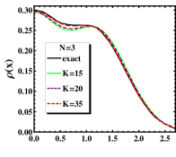
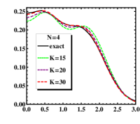
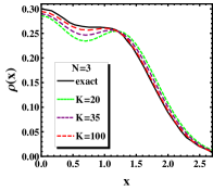
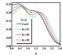
Figure 1: Profiles of one-body densities obtained for $N=3,4$ at $g=10$ for different cut-off values of $K$. Black continuous lines mark the reference results taken from [31] (Figure 2 (b-c) in this reference). The top-panel results were obtained through the optimization strategy based on the minimization of $E_{0}^{(K)}$. The corresponding numbers $D$ and the optimal values of $\Omega_{opt}$ are as follows: $\mathbf{N=3}\mathbf{:}K=15~{}(D=81,\Omega_{opt}=2.59)\mathbf{;}K=20~{}(D=148,\Omega_{opt}=3.13)\mathbf{;}K=35~{}(D=762,\Omega_{opt}=5.11)\mathbf{;}\mathbf{N=4}\mathbf{:}K=15~{}(D=136,\Omega_{opt}=1.88)\mathbf{;}K=20~{}(D=284,\Omega_{opt}=2.33)\mathbf{;}K=30~{}(D=1152,\Omega_{opt}=3.38$). The bottom-panel results were obtained at $\Omega=1$.

Black continuous lines mark the reference densities taken from [31]. For the sake of completeness, we give the optimal values of $\Omega$ in the caption to this figure. We also calculated the deviations of the approximate energies $E_{0}^{(K)}$ from the exact energies, as functions of $K$, both with and without optimization of $\Omega$. Our results for three- and four-particle calculations at two transparent values of $g$, including $g=10$, are displayed in Figure 2.

$\Omega_{0}=1$	$...$	$\Omega_{5}\approx 5.15$	$\Omega_{6}\approx 5.11$	$\Omega_{7}\approx 5.11$
$4.26943$	$...$	$4.12803$	$4.12802$	$4.12802$

Table 1: Applying Newton‘s method to the present problem yields the following recurrence equation for the term $\Omega_{n+1}$: $\Omega_{n+1}=\Omega_{n}-e^{(1)}_{n}/e^{(2)}_{n}$, where $e^{(1)}_{n}$ and $e^{(2)}_{n}$ are finite difference approximations to first and second derivatives of $E_{0}^{(K)}$ at $\Omega=\Omega_{n}$, which are calculated here with a step length of $d\Omega=0.005$. The table presents the results of the first few Newton iterations $\{\Omega_{n},E_{0}^{(K)}(\Omega_{n})\}$ obtained for the ground-state of the three-particle system with $g=10$ at $K=35$. In spite of the fact that the starting point differs considerably from an optimal solution, a fast convergence is observed.

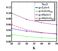
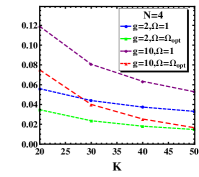
Figure 2: Relative deviations $\delta E=(E_{0}^{(K)}(\Omega)-E_{exact})/E_{exact}$ for ground states of three-and four- particle systems, calculated at $\Omega=1$ and at $\Omega=\Omega_{opt}$ for two different interaction strengths $g=2$ and $g=10$, as functions of the cut-off $K$. We have taken the reference energies $E_{exact}$ from Figure 2a in [31].

It is apparent from our results that there are clear benefits to optimizing the ED method. We can conclude from the caption to the figure 1 that the rate of convergence strongly depends on $\Omega$. In fact, the optimal value $\Omega_{opt}$ increases with the increase in $K$. As might be expected, it is clear that approximations to the energies are better after applying the optimization. This effect is more pronounced when the parameters of $g$ enter the strong-correlation regime; that is, where the true wave functions have more complex structures. However, the improvement of the convergence is more pronounced in one-body densities. For example, the exact three-particle density is well reproduced in the OED calculation when $K$ is about three times smaller than in the case where optimization is absent; that is, $K=35~{}(D=765)$ vs. $K=100~{}(D=14739)$. It should be emphasized that the calculation time in the former case (iterative minimization) was considerably shorter than in the latter one.

The optimization of $\Omega$ is therefore crucial for reducing the number of basis functions needed for accurate numerical calculations, as well as for shortening the computation time. In general, the size of the computations that can be done depends not only on the efficiency of the numerical calculation software that is used but also on the computer system itself, especially on the size of its memory. Our analysis clearly shows that the OED method consumes less memory than the standard ED approach ($\Omega=1$), and this makes it possible for systems with larger numbers of particles to be treated. Here, we leave an open question regarding how many particles can be treated effectively by modern supercomputers when using the OED approach. However, this number can be expected to be much larger than in the cases where there is no optimization of $\Omega$.

Finally, we shed some light on the applicability of the OED approach with HO eigenfunctions to systems with trapping potential that is different from the harmonic trap. Here, we consider a model of a double-well potential of the form

$${V}(x)={1\over 2}x^{2}+h\mathrm{e}^{-{x^{2}\over 2\delta^{2}}},$$ (8)

which is often used in literature to simulate different physical situations. To illustrate this, we demonstrate the convergence of the OED method for the example of a four-particle system with control parameter values: $h=4$ and $\delta=0.2$. Figure 3 shows the ground-state one-body densities for $g=4$ and $g=20$ that are obtained with the OED method for different cut-off values of $K$. In the case of $g=20$, the system enters the TG regime, and in order to confirm the validity of our calculations the results are shown along with the exact solution in the TG limit as $g\rightarrow\infty$, $\rho_{TG}(x)=1/4\sum_{i=0}^{3}\phi_{i}^{2}(x)$ [21], where $\phi_{i}$ are the solutions of the one-particle Hamiltonian with (8). Indeed, as can be seen, the limit of infinite interaction is almost reached at $g=20$. Clearly, in both cases that are considered, well-converged density profiles are obtained with moderate numbers of many-body basis functions. These results are very promising and allow us to expect that the ED method with HO eigenfunctions optimized by $\Omega$ may also be an effective tool for handling systems with more complex forms of trapping potentials, such as multi-well potentials.

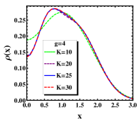
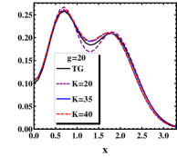
Figure 3: Profiles of the one-body densities for the four-particle system in the presence of the trapping potential (8), with $h=4$ and $\delta=0.2$, obtained for different values of the interaction strength $g$ and the cut-off $K$.

4 Conclusions

In conclusion, the ED method with an optimized basis of harmonic oscillator eigenfunctions has been tested on systems with delta interactions. Our results shows that minimization of the eigenenergy of the desired level with respect to the frequency parameter greatly improves the accuracy of the resulting approximate energy and also that of its wave function. Careful testing of the optimized ED method for harmonic and double-well potentials has proved its efficiency even in the regime of strong correlations. The use of the optimization scheme for other systems with delta interactions that are currently under intensive study, such as quantum mixtures, is a straightforward task which could also lead to many benefits.

References

- [1] A. M. Kaufman et al., Nature 527, 208 (2015)
- [2] F. Serwane et al., Science 332, 336 (2011)
- [3] M. Greiner et al., Nature 415, 39 (2002)
- [4] G. Zürn, F. Serwane et al., Phys. Rev. Lett. 108, 075303 (2012)
- [5] J. Catani et al., Phys. Rev. A 77, 011603 (2008)
- [6] G. Zürn et al., Phys. Rev. Lett. 111, 175302 (2013)
- [7] S. Murmann et al., Phys. Rev. Lett. 114, 080402 (2015)
- [8] F. Deuretzbacher, J. C. Cremon, S. M. Reimann, Phys. Rev. A 81, 063616 (2010), Erratum Phys. Rev. A 87, 039903 (2013)
- [9] S. Zöllner, H. D. Meyer, P. Schmelcher, Phys. Rev. Lett. 100, 040401 (2008)
- [10] R. E. Barfknechtet et al., At. Mol. Opt. Phys. 49, 135301 (2016)
- [11] N. L. Harshman, Phys. Rev. A 89, 033633 (2014)
- [12] P. Mujal et al., Phys. Rev. A 96, 043614 (2017)
- [13] F. Deuretzbacher et al., Phys. Rev. A 75, 013614 (2007)
- [14] S. Zöllner, H. D. Meyer, P. Schmelcher, Phys. Rev. A 78, 013629 (2008)
- [15] P. Kościk, T. Sowiński, Sci. Rep. 8, 48 (2018)
- [16] T. Sowiński et al., Phys. Rev. A 88, 033607 (2013)
- [17] M. A. Garcia-March et al., Phys. Rev. A 92, 033621 (2015)
- [18] F. F. Bellotti, A. S. Dehkharghani, N. T. Zinner, Eur. Phys. J. D 71: 37 (2017)
- [19] T. Busch et al., Found. Phys 28, 549-559 (1998)
- [20] E. H. Lieb, W. Liniger, Phys. Rev. 130, 1605 (1963)
- [21] M. Girardeau, J. Math. Phys. 1, 516 (1960)
- [22] T. Kinoshita, T. Wenger, D. S. Weiss, Science 305, 1125 (2004)
- [23] X. Yin et al., Phys. Rev. A 78, 013604 (2008)
- [24] D. S. Murphy et al., Phys. Rev. A 76, 053616 (2007)
- [25] D. S. Murphy, J. F. McCann, Phys. Rev. A 77, 063413 (2008)
- [26] B. B. Wei, S. J. Gu, H. Q. Lin, Phys. Rev. A 79, 063627 (2009)
- [27] J. Decamp et al., New J. Phys. 19, 125001 (2017)
- [28] M. D. Girardeau, A. Minguzzi, Phys. Rev. Lett. 99, 230402 (2007)
- [29] A. S. Dehkharghani, F. F. Belloti, N.T. Zinner, J. Phys. B: At. Mol. Opt. Phys. 50, 144002 (2017)
- [30] B. Fang et al., Phys. Rev. A 84 023626 (2011)
- [31] I. Brouzos, P. Schmelcher, Phys. Rev. Lett. 108, 045301 (2012)
- [32] I. Brouzos, P. Schmelcher, Phys. Rev. A, 87 023605 (2013)
- [33] R. E. Barfknecht et al. J. Phys. B: At. Mol. Opt. Phys. 49, 135301 (2016)
- [34] M. Pyzh et al., New J. Phys. 20, 15006 (2018)
- [35] H. D. Meyer, U. Manthe, L. S. Cederbaum, Chem. Phys. Lett. 165, 73 (1990)
- [36] A. I. Streltsov, O. E. Alon, L. S. Cederbaum, Phys. Rev. Lett. 99, 030402 (2007)
- [37] J. Zanghellini et al. Laser Phys. 13 1064 (2003)
- [38] L. Cao et al., J. Chem. Phys. 147, 044106 (2017)
- [39] S. Krønke et al., New J. Phys.15, 063018 (2013)
- [40] T. Grining et al., New J. Phys. 17, 115001 (2015)
- [41] T. Haugset, H. Haugerud, Phys. Rev. A 57, 3809 (1998)
- [42] Ole Søe Sørensen. Exact treatment of interacting bosons in rotating systems and lattices. PhD thesis, Aarhus University, Aarhus (2012).
- [43] M. Płodzień et al., ArXiv:1803.08387 (2018)
- [44] A. Okopińska, Phys. Rev. D 36, 1273 (1987)
- [45] N. Saad, R. L. Hall, Q. D. Katatbeh, J. Math. Phys. A 46, 022104-1 (2005)
- [46] P. Stevenson, Phys. Rev. D 23, 2961 (1981)
- [47] P. Kościk, A. Okopińska, J. Phys. A: Math. Theor. 40, 10851 (2007)