Abstract

We revisit the representation theory of the quantum double of the universal cover of the Lorentz group in 2+1 dimensions, motivated by its role as a deformed Poincaré symmetry and symmetry algebra in (2+1)-dimensional quantum gravity. We express the unitary irreducible representations in terms of covariant, infinite-component fields on curved momentum space satisfying algebraic spin and mass constraints. Adapting and applying the method of group Fourier transforms, we obtain covariant fields on (2+1)-dimensional Minkowski space which necessarily depend on an additional internal and circular dimension. The momentum space constraints turn into differential or exponentiated differential operators, and the group Fourier transform induces a star product on Minkowski space and the internal space which is essentially a version of Rieffel’s deformation quantisation via convolution.

1 Introduction

The possibility of anyonic statistics in two spatial dimensions lies at the root of the peculiarity and intricacy of planar phenomena in quantum physics, ranging from the quantum Hall effect to potential uses of anyons in topological quantum computing [1]. The mathematical origin of anyonic statistics is the infinite connectedness of the planar rotation group $\mathrm{SO}(2)$ which is topologically a circle. The goal of this paper, in brief, is to explore the consequences of this fact for quantum gravity in 2+1 dimensions, where the infinite connectedness is doubled and appears in both momentum space and the rotation group.

Our strategy in pursuing this goal is to extend and generalise the method developed in [2, 3], which proceeds from a definition of the symmetry algebra, via a covariant formulation of its irreducible unitary representations (UIRs) in momentum space to, finally, covariant fields in spacetime obeying differential or finite-difference equations. One of the upshots of our work is a construction of non-commutative plane waves for gravitational anyons via a group Fourier transform. While this transform arose in relatively recent literature in quantum gravity [4, 5, 6, 7] we note that it is essentially an example and extension of Rieffel’s deformation quantisation of the canonical Poisson structure on the dual of a Lie algebra via convolution [8].

Anyonic behaviour occurs in both non-relativistic and relativistic physics, and for the same topological reason. The proper and orthochronous Lorentz group $L_{3}^{+\uparrow}$ in 2+1 dimensions retracts to $\mathrm{SO}(2)$, and is therefore infinitely connected. Its universal cover, which cannot be realised as a matrix group, governs the properties of relativistic anyons. As we shall review, the double cover of $L_{3}^{+\uparrow}$ is the matrix group $\mathrm{SU}(1,1)$ or, equivalently, $\mathrm{SL}(2,\mathbb{R})$. In this paper, we write the universal cover as $\widetilde{\mathrm{SU}}(1,1)$.

In the spirit of Wigner’s classification of particles [9], relativistic anyons are classified by the UIRs of the universal cover of the (proper, orthochronous) Poincaré group in 2+1 dimensions, which is the semidirect product of $\widetilde{\mathrm{SU}}(1,1)$ with the group of spacetime translations. It is natural to identify the latter with the dual of the Lie algebra of $\mathrm{SU}(1,1)$. Then the universal cover of the Poincaré group is $\widetilde{\mathrm{SU}}(1,1)\ltimes\mathfrak{su}(1,1)^{*}$, with the first factor acting on the second by the co-adjoint action. While the UIRs of the Poincaré group in 2+1 dimensions are labelled by a real mass parameter and an integer spin parameter, the corresponding mass and spin parameters for the universal cover both take arbitrary real values [10]. In other words, going to the universal cover puts mass and spin on a more equal footing.

The canonical construction of the UIRs of the Poincaré group in 2+1 dimensions leads to states being realised as functions on momentum space, obeying constraints [11]. Writing these constraints in a Lorentz-covariant way, and Fourier transforming leads to standard wave equations of relativistic physics like the Klein-Gordon or Dirac equation. Relativistic wave equations for anyons have also been constructed, but for spins which are not half-integers they require infinite-component wave functions, and the derivation of the equations is not straightforward [12, 13, 14, 15].

Our treatment will naturally lead us to an equation derived via a different route by Plyushchay in [14, 15]. It makes use of the discrete series UIR of $\widetilde{\mathrm{SU}}(1,1)$, but, as pointed out by Plyushchay, it is essentially a dimensional reduction of an equation already studied by Majorana [16, 17].

The focus of this paper is a deformation of the universal cover of the Poincaré group to a quantum group which arises in (2+1)-dimensional quantum gravity. In 2+1 dimensions, there are no propagating gravitational degrees of freedom, and the phase space of gravity interacting with a finite number of particles and in a universe where spatial slices are either compact or accompanied by suitable boundary conditions at spatial infinity is finite-dimensional. In those cases where the resulting phase space could be quantised, the Hilbert space of the quantum theory can naturally be constructed out of unitary representations of the quantum double of $L_{3}^{+\uparrow}$ or one of its covers [18, 19, 20]. In a sense that can be made precise, this double is a deformation of the Poincaré group in 2+1 dimensions [21, 22], with the linear momenta in $\mathfrak{su}(1,1)^{*}$ (the generators of translations) being replaced by functions on $L_{3}^{+\uparrow}$ or one of its covers.

In the quantum double of $L_{3}^{+\uparrow}$, Lorentz transformations and translation are implemented via Hopf algebras which are in duality, namely the group algebra of $L_{3}^{+\uparrow}$ and the dual algebra of functions on $L_{3}^{+\uparrow}$. The quantum double is a ribbon Hopf algebra whose $R$-matrix can be given explicitly. The unitary irreducible representations describing massive particles are labelled by an integer spin and a mass parameter taking values on a circle.

In analogy with the treatment of the Poincaré group, one could define the universal cover of the double of $L_{3}^{+\uparrow}$ by replacing the group algebra of the Lorentz group with the group algebra of the universal cover $\widetilde{\mathrm{SU}}(1,1)$. There are indications that this is required when applying the quantum double to quantum gravity in 2+1 dimensions. In particular, several independent arguments lead to the conclusion that, in (2+1)-dimensional gravity, the spin $s$ is quantised in units which depends on its mass $m$ according to

$$s=\frac{n}{1-\frac{\mu}{2\pi}},$$ (1.1)

where $n\in\mathbb{Z}$, $\mu=8\pi mG$ and $G$ is Newton’s gravitational constant, see [22, 23].

Covering the Lorentz transformations without changing the momentum algebra would destroy the duality between the two. It is therefore more natural to also consider a universal covering of the momentum algebra, i.e., to identify the momentum algebra with the function algebra on $\widetilde{\mathrm{SU}}(1,1)$. The resulting quantum double of the universal cover of the Lorentz group, called Lorentz double in [22], is a ribbon-Hopf algebra and has UIRs describing massive particles which are labelled by a spin parameter $s$ and a mass parameter $\mu$ for which (1.1) makes sense.

In this paper, we consider the Lorentz double and derive a new formulation of its UIRs in terms of infinite-component functions on momentum space $\widetilde{\mathrm{SU}}(1,1)$ obeying Lorentz-covariant constraints. We extend and use the notion of group Fourier transforms [4, 5, 6, 7] to derive covariant wave equations on Minkowski space equipped with a $\star$-product.

Our method extends earlier work in [3] where analogous relativistic wave equations for massive particles were obtained from the UIRs of the quantum double of the Lorentz group. The transition to the universal cover poses two separate challenges. Our wave functions in momentum space now live on $\widetilde{\mathrm{SU}}(1,1)$, and they take values in infinite-dimensional UIRs of $\widetilde{\mathrm{SU}}(1,1)$ called the discrete series. The change in momentum space leads to a particularly natural version of the group Fourier transform, essentially because group-valued momenta can be parametrised bijectively via the exponential map and one additional integer label. In order to include the integer in our Fourier transform we are forced to introduce a dual circle on the spacetime side. The emergence of a compact additional dimension is a remarkable and intriguing aspect of our construction.

Fourier transforming the algebraic spin and mass constraints from momentum space to Minkowski space produces equations on non-commutative Minkowski space which involve either differential operators or the exponential of a first-order differential operator. We end the paper with a short discussion of these non-commutative wave equations for gravitational anyons, leaving a detailed study for future work. Non-commutative waves for anyons have previously been discussed in the literature [24]. However, the discussion there is in the context of non-relativistic limits rather than the inclusion of gravity, and the mathematics is rather different.

The paper is organised as follows. In Sect. 2, we introduce our notation and review the definition and parametrisation of the universal cover $\widetilde{\mathrm{SU}}(1,1)$ as well as the discrete series UIRs. We also revisit the UIRs of the Poincaré group and briefly summarise the covariantisation of the UIRs and their Fourier transform, following [3]. In Sect. 3, we generalise the covariantisation procedure to the universal cover of the Poincaré group, thus obtaining wave equations for infinite-component anyonic wave functions. Our version of these equations is essentially that considered by Plyushchay [14, 15] but our derivation of them appears to be new. Sect. 4 extends the analysis to the Lorentz double. We derive a Lorentz-covariant form of the UIRs, and point out that one of the defining constraints, called the spin constraint, can be expressed succinctly in terms of the ribbon element of the Lorentz double. The group Fourier transform on $\widetilde{\mathrm{SU}}(1,1)$ requires a parametrisation of this group via the exponential map, and we discuss this in some detail. We use the Fourier transform to derive non-commutative wave equations, and then use the short final Sect. 5 to discuss our results and to point out avenues for further research.

2 Poincaré symmetry and massive particles in 2+1 dimensions

We review the symmetry group of (2+1)-dimensional Minkowski space: its Lie algebra, its various covering groups and their representation theory. Unfortunately there is no single book or paper which covers these topics in conventions which are convenient for our purposes. We therefore adopt a mixture of the conventions in the papers [22] and [3] and the book [25], which are key references for us.

2.1 Minkowski space and the double cover of the Poincaré group

We denote $(2+1)$ dimensional Minkowski space by $\mathbb{R}^{2,1}$, with the convention that the Minkowski metric is mostly minus. Vectors in $\mathbb{R}^{2,1}$ will be denoted by ${\mbox{\boldmath$x$}}=(x^{0},x^{1},x^{2})$, with Latin indices for components and the inner product given by

$$\eta({\mbox{\boldmath$x$}},{\mbox{\boldmath$y$}})=\eta_{ab}x^{a}y^{b}=x^{0}y^{0}-x^{1}y^{1}-x^{2}y^{2}.$$ (2.1)

The group of linear transformations that leave $\eta$ invariant is the Lorentz group $L_{3}=O(2,1)$. This group has four connected components, but we are mainly interested in the component connected to the identity, i.e., the subgroup of proper orthochronous Lorentz transformations, denoted $L_{3}^{+\uparrow}$.

The group of affine transformations that leave the Minkowski metric invariant is the semi-direct product $L_{3}\ltimes\mathbb{R}^{3}$ of the Lorentz group with the abelian group of translations. We call its identity component Poincaré group and denote it as

$$P_{3}=L_{3}^{+\uparrow}\ltimes\mathbb{R}^{3}.$$ (2.2)

The Lie algebra $\mathfrak{p}_{3}$ of the Poincaré group is spanned by rotation and boost generators $J^{0},J^{1},J^{2}$, and time and space translation generators $P_{0},P_{1},P_{2}$. They can be chosen so that the commutators are

$$[J^{a},J^{b}]=\epsilon^{abc}J_{c},\quad[J_{a},P_{b}]=\epsilon_{abc}P^{c},\quad[P_{a},P_{b}]=0.$$ (2.3)

Here and in the following $\epsilon_{abc}$ is the totally antisymmetric tensor with $\epsilon_{012}=1$, and indices are raised and lowered with the Minkowski metric $\eta=\text{diag}(1,-1,-1)$. Note that this means in particular that $-J^{0}$ is the generator of mathematically positive rotations in momentum space. This affects our conventions for the sign of the spin later in this paper.

In quantum mechanics, classical symmetries described by a Lie group $G$ are implemented by projective representations, which, in the case of the Lorentz group, may equivalently be described by unitary representations of the universal covering group. In the case of relativistic symmetries in 3+1 dimensions the universal cover of the Lorentz group is its double cover and is isomorphic to $\mathrm{SL(2,\mathbb{C})}$. In 2+1 dimensions the double cover of $L_{3}^{+\uparrow}$ is isomorphic to $\mathrm{SL}(2,\mathbb{R})$ or, equivalently, $\mathrm{SU}(1,1)$, but this is not the universal cover. Therefore a choice has to be made as to which covering group one should implement in the quantum theory. The paper [3], to which we will refer frequently for details, works with the double cover in the realisation $\mathrm{SL}(2,\mathbb{R})$.

We will consider the universal cover here. For our purposes it is more convenient to first consider the double cover $\mathrm{SU}(1,1)$ because it allows for an easy transition to the universal cover. In order to translate results from [3], the reader will need to apply the unitary matrix

$$h=\frac{1}{2}\begin{pmatrix}1+i&-1-i\\ 1-i&\phantom{-}1-i\end{pmatrix},$$ (2.4)

which conjugates $\mathrm{SL}(2,\mathbb{R})$ into $\mathrm{SU}(1,1)$ within $\mathrm{SL}(2,\mathbb{C})$, i.e., $h^{-1}\mathrm{SL}(2,\mathbb{R})h=\mathrm{SU}(1,1)$.

We use the following basis of the Lie algebra $\mathfrak{su}(1,1)$

$$s^{0}=-\frac{i}{2}\sigma_{3}=\begin{pmatrix}-\frac{i}{2}&0\\ \phantom{-}0&\frac{i}{2}\end{pmatrix},\quad s^{1}=-\frac{1}{2}\sigma_{1}=\begin{pmatrix}\phantom{-}0&-\frac{1}{2}\\ -\frac{1}{2}&\phantom{-}0\end{pmatrix},\quad s^{2}=\frac{1}{2}\sigma_{2}=\begin{pmatrix}0&-\frac{i}{2}\\ \frac{i}{2}&\phantom{-}0\end{pmatrix},$$ (2.5)

which are normalised to have the commutation relations of the Lorentz part of (2.3):

$$[s_{a},s_{b}]=\epsilon_{abc}s^{c}.$$ (2.6)

The basis $t^{a}$, $a=0,1,2,$ of $\mathfrak{sl}(2,\mathbb{R})$ used in [3] is related to our basis of $\mathfrak{su}(1,1)$ via $s^{a}=h^{-1}t^{a}h.$

An arbitrary matrix $M\in\mathrm{SU}(1,1)$ can be parametrised in terms of two complex numbers $a,b$ which satisfy $|a|^{2}-|b|^{2}=1$ via

$$M=\begin{pmatrix}a&\bar{b}\\ b&\bar{a}\end{pmatrix}.$$ (2.7)

However, a more convenient parametrisation for the extension to the universal cover is obtained by introducing an angular coordinate $\omega\in[0,4\pi)$ and a complex number $\gamma=b/a$ of modulus $|\gamma|<1$ so that

$$a=\frac{1}{\sqrt{1-|\gamma|^{2}}}e^{i\frac{\omega}{2}},\qquad b=\frac{\gamma}{\sqrt{1-|\gamma|^{2}}}e^{i\frac{\omega}{2}}.$$ (2.8)

Using this parametrisation, one can see that $\mathrm{SU}(1,1)$ is topologically the open solid torus $S^{1}\times D$, where $D$ is the open unit disk. Note that an $\mathrm{SU}(1,1)$ element parametrised via (2.8) can be written as

$$M(\omega,\gamma)=\frac{1}{\sqrt{1-|\gamma|^{2}}}\begin{pmatrix}e^{i\frac{\omega}{2}}&\bar{\gamma}e^{-i\frac{\omega}{2}}\\ \gamma e^{i\frac{\omega}{2}}&e^{-i\frac{\omega}{2}}\end{pmatrix}=\frac{1}{\sqrt{1-|\gamma|^{2}}}\begin{pmatrix}1&\bar{\gamma}\\ \gamma&1\end{pmatrix}\begin{pmatrix}e^{i\frac{\omega}{2}}&0\\ 0&e^{-i\frac{\omega}{2}}\end{pmatrix}.$$ (2.9)

We will need to understand the conjugacy classes of $\mathrm{SU}(1,1)$ for various applications in this paper. These are obtained from the well-known conjugacy classes of $\mathrm{SL}(2,\mathbb{R})$ (see [3], for example) by conjugation with $h$ and therefore determined by the trace (which, for determinant one, fixes the eigenvalues up to ordering) plus additional data. Elements $u\in\mathrm{SU}(1,1)$ with absolute value of the trace less than 2 are called elliptic elements. They are conjugate to rotations of the form

$$\begin{pmatrix}e^{i\frac{\alpha}{2}}&0\\ 0&e^{-i\frac{\alpha}{2}}\end{pmatrix},\quad\alpha\in(0,2\pi)\cup(2\pi,4\pi).$$ (2.10)

Each value of $\alpha$ labels one conjugacy class (so there are two conjugacy classes for each value of the trace). Elements with absolute value of the trace equal to 2 include $\pm\text{id}$ (forming a conjugacy class each) and parabolic elements, which are conjugate to

$$\begin{pmatrix}\pm 1-i\zeta&\zeta\\ \zeta&\pm 1+i\zeta\end{pmatrix},\quad\zeta\in(-\infty,0)\cup(0,\infty).$$ (2.11)

Each choice of sign on the diagonal and each value of $\zeta$ labels one conjugacy class. Element with absolute value of the trace greater than two are called hyperbolic. They are conjugate to

$$\pm\begin{pmatrix}\cosh\xi&\sinh\xi\\ \sinh\xi&\cosh\xi\end{pmatrix},\quad\xi\in(0,\infty).$$ (2.12)

Each choice of sign and each value of $\xi$ determines one conjugacy class (negative values are not needed since conjugation with $\sigma_{3}\in\mathrm{SU}(1,1)$ flips the sign).

The double cover of the Poincaré group is

$$\tilde{P}_{3}\simeq\mathrm{SU}(1,1)\ltimes\mathbb{R}^{3},$$ (2.13)

but for our purposes it is natural to identify the translation subgroup with the vector space $\mathfrak{su}(1,1)^{*}$, and to view $\tilde{P}_{3}$ as

$$\tilde{P}_{3}\simeq\mathrm{SU(1,1)}\ltimes\mathfrak{su}(1,1)^{*},$$ (2.14)

with $\mathrm{SU(1,1)}$ acting on translations via the co-adjoint action $\mbox{Ad}^{*}$. More precisely, the product of elements $(g_{1},a_{1}),(g_{2},a_{2})\in\tilde{P}_{3}$ in the conventions of [3, 2] is

$$(g_{1},a_{1})(g_{2},a_{2})=(g_{1}g_{2},\mbox{Ad}^{*}_{g_{2}}a_{1}+a_{2}).$$ (2.15)

The motivation for the interpretation (2.14) of the double cover of the Poincaré group comes from the formulation of 3d gravity as a Chern-Simons theory with the Poincaré group as a gauge group. This requires an invariant and non-degenerate pairing on $\mathfrak{p}_{3}$. The, up to scale, a unique such pairing is the dual pairing between the Lorentz generators and the translation generators, i.e., the canonical pairing on the Lie algebra

$$\mathfrak{p}_{3}=\mathfrak{su}(1,1)\oplus\mathfrak{su}(1,1)^{*}.$$ (2.16)

As remarked in [3] and for the Euclidean case in [2], the dual basis of the translation generators $P_{a}$ (now viewed as a basis of $\mathfrak{su}(1,1)^{*}$) may have a different normalisation to the basis ${s^{a}}$ which is fixed by the commutation relations (2.5) . Adapting the conventions of [2, 3], and working with the generators $s^{a}$ for $\mathfrak{su}(1,1)$, we write the pairing in our basis as

$$\langle s_{a},P_{b}\rangle=-\frac{1}{\lambda}\eta_{ab},$$ (2.17)

where the scale $\lambda$ is a constant of dimension inverse mass. In the context of 2+1 gravity it is related to Newton’s gravitational constant $G$ via $\lambda=8\pi G$.

With the usual identification of momentum space as the dual of spacetime translations, momenta $p$ in 2+1 dimensions now naturally live in $(\mathfrak{su}(1,1)^{*})^{*}\simeq\mathfrak{su}(1,1)$. For consistency with (2.17) we set

$$P^{*a}=-\lambda s^{a},$$ (2.18)

so that a general element $p$ of momentum space may be expressed as

$$p=p_{a}P^{*a}=-\lambda p_{a}s^{a}.$$ (2.19)

The reason for inserting a minus sign here is that $-s^{0}$ generates mathematically positive rotation, as mentioned after (2.3).

While the pairing between Lorentz and translation generators is canonical (up to scale), the inner product between two momenta $p$ and $q$ in $\mathfrak{su}(1,1)$ requires the trace. We define the inner product as

$$-\frac{2}{\lambda^{2}}\text{tr}(pq)=p_{a}q^{a}.$$ (2.20)

This is invariant under the (adjoint) action of $\mathrm{SU(1,1)}$. Using the convention to mark coordinate vectors by bold letters we write

$${\mbox{\boldmath$p$}}\cdot{\mbox{\boldmath$q$}}=p_{a}q^{a},$$ (2.21)

and occasionally also

$${\mbox{\boldmath$p$}}\cdot{\mbox{\boldmath$s$}}=p_{a}s^{a}.$$ (2.22)

We also require a notation for the absolute value of the norm of $p$. We write this as

$$|{\mbox{\boldmath$p$}}|=\sqrt{|{\mbox{\boldmath$p$}}\cdot{\mbox{\boldmath$p$}}|}.$$ (2.23)

As pointed out in the Introduction, $\mathrm{SU(1,1)}$ and its universal cover both play two mutually dual roles in this paper as Lorentz symmetry and as curved momentum space. In the latter context we will require one further parametrisation of ${\mathrm{SU}}(1,1)$, namely the one obtained via the exponential map. By ‘conjugating’ the detailed discussion of the corresponding parametrisation of $\mathrm{SL}(2,\mathbb{R})$ in [3] with (2.4), one checks that any element $u\in{\mathrm{SU}}(1,1)$ can, up to a sign, be written as the exponential of the Lie-algebra valued momentum $p$, i.e.,

$$u=\pm\exp(p).$$ (2.24)

We will revisit this fact and its geometrical interpretation in Sect. 4. In that context we will also need the following explicit form of the exponential:

$$\exp(-\lambda p_{a}s^{a})=c(|{\mbox{\boldmath$p$}}|)\,\text{id}-2s(|{\mbox{\boldmath$p$}}|)\hat{p}\cdot{\mbox{\boldmath$s$}},$$ (2.25)

where we introduced the function

$$s(|{\mbox{\boldmath$p$}}|)=\begin{cases}\sin\left(\lambda\frac{|{\mbox{\boldmath$p$}}|}{2}\right)\;&\text{if}\;{\mbox{\boldmath$p$}}^{2}>0\\ \lambda\;&\text{if}\;{\mbox{\boldmath$p$}}^{2}=0\\ \sinh\left(\lambda\frac{|{\mbox{\boldmath$p$}}|}{2}\right)\;&\text{if}\;{\mbox{\boldmath$p$}}^{2}<0\end{cases}\quad\text{and}\quad c(|{\mbox{\boldmath$p$}}|)=\begin{cases}\cos\left(\lambda\frac{|{\mbox{\boldmath$p$}}|}{2}\right)\;&\text{if}\;{\mbox{\boldmath$p$}}^{2}>0\\ 1\;&\text{if}\;{\mbox{\boldmath$p$}}^{2}=0\\ \cosh\left(\lambda\frac{|{\mbox{\boldmath$p$}}|}{2}\right)\;&\text{if}\;{\mbox{\boldmath$p$}}^{2}<0\end{cases},$$ (2.26)

as well as the generalised unit-vector

$$\hat{p}=\begin{cases}\frac{{\mbox{\boldmath$p$}}}{|{\mbox{\boldmath$p$}}|}\;&\text{if}\;{\mbox{\boldmath$p$}}^{2}\neq 0\\ {\mbox{\boldmath$p$}}\;&\text{if}\;{\mbox{\boldmath$p$}}^{2}=0\end{cases}.$$ (2.27)

The functions $s$ and $c$ satisfy a generalised version of the Pythagorean formula:

$$c^{2}(|{\mbox{\boldmath$p$}}|)+\hat{p}^{2}s^{2}(|{\mbox{\boldmath$p$}}|)=1.$$ (2.28)

2.2 The universal cover the Lorentz group and the discrete series representation

In this paper we shall consider anyonic particles and for this we will need to work with the universal cover of the Poincaré group which we denote by $P^{\infty}_{3}$:

$$P^{\infty}_{3}=\widetilde{\mathrm{SU}}(1,1)\ltimes\mathfrak{su}(1,1)^{*},$$ (2.29)

where $\widetilde{\mathrm{SU}}(1,1)$ is the universal cover of $\mathrm{SU}(1,1)$. The group $\widetilde{\mathrm{SU}}(1,1)$ is not a matrix group, but, as we will explain in some detail below, its elements are conveniently parametrised by a real number $\omega$ and complex number $\gamma$ of modulus less than $1$. Thus we write elements of $\widetilde{\mathrm{SU}}(1,1)$ as pairs $(\omega,\gamma)$ and elements of $P^{\infty}_{3}$ as pairs $((\omega,\gamma),a)$, with $a\in\mathfrak{su}(1,1)^{*}$, so that the product is

$$((\omega_{1},\gamma_{1}),a_{1})((\omega_{2},\gamma_{2}),a_{2})=((\omega_{1},\gamma_{1})(\omega_{2},\gamma_{2}),\mbox{Ad}^{*}_{(\omega_{2},\gamma_{2})}a_{1}+a_{2}).$$ (2.30)

The universal cover of $\mathrm{SU}(1,1)\simeq S^{1}\times D$, denoted $\widetilde{\mathrm{SU}}(1,1)$, is diffeomorphic to the product $\mathbb{R}\times D$, where the circle factor $S^{1}$ has been covered by the real line. We extend our parametrisation (2.9) of $\mathrm{SU}(1,1)$ to the universal cover by simply allowing the angular variable $\omega$ to take values in $\mathbb{R}$. We then identify elements of $\widetilde{\mathrm{SU}}(1,1)$ with pairs $(\omega,\gamma)\in\mathbb{R}\times D$. The product $(\omega_{1},\gamma_{1})(\omega_{2},\gamma_{2})$ is the element $(\omega,\gamma)$ given by an analytic extension of the formulae one obtains when writing the matrix product of elements of the form (2.9) in terms of the parameters:

$$\gamma =(\gamma_{1}+\gamma_{2}e^{-i\omega_{1}})(1+\bar{\gamma}_{1}\gamma_{2}e^{-i\omega_{1}})^{-1}$$

$$\omega =\omega_{1}+\omega_{2}+\frac{1}{i}\ln\left(\frac{1+\bar{\gamma}_{1}\gamma_{2}e^{-i\omega_{1}}}{1+\gamma_{1}\bar{\gamma_{2}}e^{i\omega_{1}}}\right).$$ (2.31)

Here the logarithms of the form $\ln(1+w)$ are defined in terms of the usual (Mercator) power series, which returns the principal value of $\ln(1+w)$. With $\gamma_{1}$ and $\gamma_{2}$ inside the unit disk, this means in particular

$$\frac{1}{i}\ln\left(\frac{1+\bar{\gamma}_{1}\gamma_{2}e^{-i\omega_{1}}}{1+\gamma_{1}\bar{\gamma_{2}}e^{i\omega_{1}}}\right)\in\left(-\pi,\pi\right).$$ (2.32)

We also note that

$$(\omega,\gamma)^{-1}=(-\omega,-e^{i\omega}\gamma).$$ (2.33)

In terms of the coordinates $(\omega,\gamma)$, the canonical projection

$$\pi:\widetilde{\mathrm{SU}}(1,1)\rightarrow\mathrm{SU}(1,1)$$ (2.34)

is simply the map

$$\pi:(\omega,\gamma)\mapsto M(\omega,\gamma),$$ (2.35)

where it is clear from (2.9) that the right hand side only depends on $\omega$ mod $4\pi$. This is a homomorphism whose kernel is the central subgroup generated by the element $(4\pi,0)$. It is, however, convenient to introduce a special name for rotations by $2\pi$. With

$$\Omega=(2\pi,0)\in\widetilde{\mathrm{SU}}(1,1),$$ (2.36)

we have $\pi(\Omega)=-\text{id}$ and

$$\text{ker}\;\pi=\{\Omega^{2n}|n\in\mathbb{Z}\}.$$ (2.37)

When working with the Lie algebra of $\widetilde{\mathrm{SU}}(1,1)$ we will continue to use the notation $s^{a}$, $a=0,1,2$, for the generators, i.e., we identify the Lie algebra of $\widetilde{\mathrm{SU}}(1,1)$ with its image under the differential of the projection (2.34). However, the exponential of these generators $\widetilde{\mathrm{SU}}(1,1)$ cannot be computed via matrix exponentials; instead one has to use the differential geometric definition in terms of the geodesic flow with respect to the bi-invariant (Lorentzian) metric on $\widetilde{\mathrm{SU}}(1,1)$. We will need to exponentiate timelike, lightlike and spacelike generators at various points in this paper, and therefore note the relevant expressions here. Since the geometric definition coincides with the matrix exponential for $\mathrm{SU}(1,1)$, the results are essentially analytic continuations of the expressions for $\mathrm{SU}(1,1)$ in the variable $\omega$. With the notation

$$\exp:\mathfrak{su}(1,1)\rightarrow\mathrm{SU}(1,1),\qquad\widetilde{\exp}:\mathfrak{su}(1,1)\rightarrow\widetilde{\mathrm{SU}}(1,1),$$ (2.38)

for the exponential maps, we note exponentials of typical timelike, spacelike and lightlike elements in the Lie algebra. They give rise to, respectively, elliptic, hyperbolic and parabolic elements in the group, as exhibited in (2.10), (2.11) and (2.12).

$$\exp(-\alpha s^{0}) =\begin{pmatrix}e^{i\frac{\alpha}{2}}&0\\ 0&e^{-i\frac{\alpha}{2}}\end{pmatrix}, \widetilde{\exp}(-\alpha s^{0}) =(\alpha,0),$$ (2.39)

$$\exp(-2\xi s^{1}) =\begin{pmatrix}\cosh\xi&\sinh\xi\\ \sinh\xi&\cosh\xi\end{pmatrix}, \widetilde{\exp}(-2\xi s^{1}) =\left(0,\tanh\xi\right),$$

$$\exp(2\zeta(s^{0}-s^{1})) =\begin{pmatrix}1-i\zeta&\zeta\\ \zeta&1+i\zeta\end{pmatrix}, \widetilde{\exp}(2\zeta(s^{0}-s^{1})) =\left(-2\tan^{-1}(\zeta),\frac{\zeta}{1-i\zeta}\right).$$

Bearing in mind the comment made after (2.3), we note in particular that the adjoint action of $(\alpha,0)$ on momentum space induces a mathematically positive rotation.

The unitary irreducible representations (UIRs) of $\widetilde{\mathrm{SU}}(1,1)$ have been classified into a number of infinite families and are given in detail in [25] and also [10]. The particular class that is used to model anyonic particles in [13, 14, 15] is called the discrete series. We briefly review this here, using [25] as a main reference but adapting notation used in [10]. In particular, we label the UIRs in the discrete series by $l\in\mathbb{R}^{+}$ and a sign.

The carrier spaces for the discrete series are given by the space of suitably completed holomorphic ($+$) or anti-holomorphic ($-$) functions on the open unit disk. These spaces will be denoted $\mathcal{H}_{l\pm}$ or simply $\mathcal{H}$ when no confusion can arise. The completion is with respect to the appropriate Hilbert space inner product given below. For the family ($l+$), the inner product between two holomorphic functions $f=\sum_{n=0}\alpha_{n}z^{n}$ and $g=\sum_{n=0}\beta_{n}z^{n}$ is

$$\left(f,g\right)_{l}=\sum_{n=0}^{\infty}\frac{\Gamma(2l)\Gamma(n+1)}{\Gamma(2l+n)}\alpha_{n}\bar{\beta}_{n},$$ (2.40)

where $\Gamma$ is the Gamma function. The inner product above may be given an integral expression for the case $l>\frac{1}{2}$ as

$$\left(f,g\right)_{l\,>\frac{1}{2}}=\frac{2l-1}{\pi}\int_{D}(1-\lvert z\rvert^{2})^{2(l-1)}f(z)\bar{g(z)}\;\frac{i}{2}\mathrm{d}z\wedge\mathrm{d}\bar{z}.$$ (2.41)

For the representations labelled by $l-$ the inner products is as above except that the functions $f$ and $g$ are anti-holomorphic and therefore given as power series of the form $f=\sum_{n=0}\alpha_{n}\bar{z}^{n}$ and $g=\sum_{n=0}\beta_{n}\bar{z}^{n}$.

In order to express the action of $\widetilde{\mathrm{SU}}(1,1)$ on $\mathcal{H}$ for these representations we recall the projection map (2.35) and (2.9), and combine it with a right action of $\mathrm{SU}(1,1)$ on the open unit disk:

$$z\cdot\begin{pmatrix}a&\bar{b}\\ b&\bar{a}\end{pmatrix}=\frac{az+b}{\bar{b}z+\bar{a}}=e^{i\omega}\frac{z+\gamma}{\bar{\gamma}z+1}.$$ (2.42)

The action of $\widetilde{\mathrm{SU}}(1,1)$ on the carrier space $\mathcal{H}_{l+}$ is

$$(D_{l+}(\omega,\gamma)f)(z)=e^{il\omega}(1-\lvert\gamma\rvert^{2})^{l}(1+\bar{\gamma}z)^{-2l}f(z\cdot\pi(\omega,\gamma)).$$ (2.43)

On $\mathcal{H}_{l-}$ it is

$$(D_{l-}(\omega,\gamma)f)(\bar{z})=e^{-il\omega}(1-\lvert\gamma\rvert^{2})^{l}(1+\gamma\bar{z})^{-2l}f(\overline{z\cdot\pi(\omega,\gamma)}).$$ (2.44)

The above action simplifies in the case $l\in\frac{1}{2}\mathbb{N}$, where one recovers a genuine representation of the group $\mathrm{SU}(1,1)$. In this case, one can use (2.8) to write

$$(D_{l+}(\omega,\gamma)f)(z)=(\bar{a}+\bar{b}z)^{-2l}f(z\cdot\pi(\omega,\gamma)),$$ (2.45)

and

$$(D_{l-}(\omega,\gamma)f)(\bar{z})=(a+b\bar{z})^{-2l}f(\overline{z\cdot\pi(\omega,\gamma)}).$$ (2.46)

A canonical choice of basis in $\mathcal{H}_{l+}$ is given by the orthonormal functions

$$e^{+}_{n,l}(z)=\left(\frac{\Gamma(2l+n)}{\Gamma(2l)\Gamma(n+1)}\right)^{\frac{1}{2}}z^{n},\;\;n\in\mathbb{N},$$ (2.47)

and for $\mathcal{H}_{l-}$ we have the basis

$$e^{-}_{n,l}(\bar{z})=\left(\frac{\Gamma(2l+n)}{\Gamma(2l)\Gamma(n+1)}\right)^{\frac{1}{2}}\bar{z}^{n},\;\;n\in\mathbb{N}.$$ (2.48)

The state for $n=0$ in both $(l,+)$ and $(l,-)$ is the constant function. It plays an important role in constructing a covariant descriptions of UIRs, so we introduce the notation

$$\Ket{0}_{l}=e^{+}_{0,l}=e^{-}_{0,l}$$ (2.49)

for the map $z\mapsto 1$.

In these representations the infinitesimal generators of the Lie algebra, denoted $d_{l\pm}(s^{a})$, can be realised as differential operators acting on the carrier space $\mathcal{H}$. Starting with the usual definition

$$d_{l\pm}(s^{a})=\left.\frac{\mathrm{d}}{\mathrm{d}\epsilon}\right\rvert_{\epsilon=0}D_{l\pm}(\widetilde{\exp}{\epsilon s^{a}}),$$ (2.50)

we compute for the positive discrete series

$$d_{l+}(s^{0}) =-il-iz\frac{\mathrm{d}}{\mathrm{d}z},$$

$$d_{l+}(s^{1}) =lz-\frac{1}{2}(1-z^{2})\frac{\mathrm{d}}{\mathrm{d}z},$$

$$d_{l+}(s^{2}) =ilz+\frac{i}{2}(1+z^{2})\frac{\mathrm{d}}{\mathrm{d}z},$$ (2.51)

and for the negative series

$$d_{l-}(s^{0}) =il+i\bar{z}\frac{\mathrm{d}}{\mathrm{d}\bar{z}},$$

$$d_{l-}(s^{1}) =l\bar{z}-\frac{1}{2}(1-\bar{z}^{2})\frac{\mathrm{d}}{\mathrm{d}\bar{z}},$$

$$d_{l-}(s^{2}) =-il\bar{z}-\frac{i}{2}(1+\bar{z}^{2})\frac{\mathrm{d}}{\mathrm{d}\bar{z}}.$$ (2.52)

For later use, we note that the linear combination $s^{a}p_{a}$ for an arbitrary vector $p$ acts according to

$$d_{l+}(s^{a})p_{a}=-ilp_{0}+i(p_{2}-ip_{1})lz+i\left(\frac{1}{2}(p_{2}+ip_{1})-p_{0}z+\frac{1}{2}(p_{2}-ip_{1})z^{2}\right)\frac{\mathrm{d}}{\mathrm{d}z},$$ (2.53)

and

$$d_{l-}(s^{a})p_{a}=ilp_{0}-i(p_{2}+ip_{1})l\bar{z}-i\left(\frac{1}{2}(p_{2}-ip_{1})-p_{0}\bar{z}+\frac{1}{2}(p_{2}+ip_{1})\bar{z}^{2}\right)\frac{\mathrm{d}}{\mathrm{d}\bar{z}}.$$ (2.54)

The vector fields appearing in the action of the $s^{a}p_{a}$ have a natural geometrical interpretation which is familiar in the context of the mini-twistor correspondence between points in Euclidean 3-space and the set of all the lines through that point. We explain briefly how this point of view fits into our Lorentzian setting.

We can parametrise the set of all timelike lines in 2+1 dimensional Minkowski space in terms of a timelike vector $q$, normalised so that ${\mbox{\boldmath$q$}}^{2}=1$ and giving the direction of the line, and a vector $k$ which lies on the line and which can be chosen to satisfy ${\mbox{\boldmath$k$}}\cdot{\mbox{\boldmath$q$}}=0$ without loss of generality. Geometrically, $q$ lies on the two-sheeted hyperboloid, and $k$ lies in the tangent space at $q$.

In terms of an orthonormal basis ${\mbox{\boldmath$e$}}^{0},{\mbox{\boldmath$e$}}^{1},{\mbox{\boldmath$e$}}^{2}$ of Minkowski space, and the complex linear combination ${\mbox{\boldmath$e$}}={\mbox{\boldmath$e$}}^{1}+i{\mbox{\boldmath$e$}}^{2}$, we can parametrise $q$ in terms of a complex variable $z$ in the unit disk via

$${\mbox{\boldmath$q$}}=\frac{1}{1-|z|^{2}}\left((1+|z|^{2}){\mbox{\boldmath$e$}}^{0}+z\bar{{\mbox{\boldmath$e$}}}+\bar{z}{\mbox{\boldmath$e$}}\right),$$

and the tangent vector $k$ in terms of a complex number $w$ via

$${\mbox{\boldmath$k$}}=w\frac{\partial{\mbox{\boldmath$q$}}}{\partial z}+\bar{w}\frac{\partial{\mbox{\boldmath$q$}}}{\partial\bar{z}}=\frac{1}{(1-|z|^{2})^{2}}\left(2(w\bar{z}+\bar{w}z){\mbox{\boldmath$e$}}^{0}+(\bar{w}+w\bar{z}^{2}){\mbox{\boldmath$e$}}+(w+\bar{w}z^{2})\bar{\mbox{\boldmath$e$}}\right).$$

Then one checks that the point ${\mbox{\boldmath$p$}}=p_{0}{\mbox{\boldmath$e$}}^{0}+p_{2}{\mbox{\boldmath$e$}}^{1}+p_{1}{\mbox{\boldmath$e$}}^{2}$ lies on the line through $k$ and in the direction $q$ if and only if

$$w=\frac{1}{2}(p_{2}+ip_{1})-p_{0}z+\frac{1}{2}(p_{2}-ip_{1})z^{2}.$$ (2.55)

In other words, the derivatives appearing in (2.53) and (2.54) are precisely the holomorphic and anti-holomorphic part of the tangent vector which characterises a line containing $p$ and in the direction $q$ determined by $z$.

2.3 Massive $\tilde{P}_{3}$ representations

There are various ways of getting from the UIRs of the Poincaré group to the covariant wave equations of relativistic physics. In [2, 3], a procedure was developed which is also effective when the Poincaré group is deformed to the quantum double of the Lorentz group or one of its covers. We briefly review the method here in a convenient form for extension to the anyonic case. However, relative to [3] we change the sign convention for mass and spin to agree with the one used in [22].

Using the isomorphism $\tilde{P}_{3}\simeq\mathrm{SU}(1,1)\ltimes\mathfrak{su}(1,1)^{*}$ in (2.14), UIRs of $\tilde{P}_{3}$ may be classified by the adjoint orbits of $\mathrm{SU(1,1)}$ in momentum space $\mathfrak{su}(1,1)$ together with an UIR of associated stabiliser groups. For massive particles, the former encodes the mass, and the latter its spin. In the case of a particle of mass $m\neq 0$, we denote the adjoint orbit by $O^{T}_{m}$. It elements are obtained by boosting the representative momentum $-\lambda ms^{0}$ (which generates a mathematically positive rotation) to obtain the typical element

$$p=-v\lambda ms^{0}v^{-1}=-\lambda{\mbox{\boldmath$p$}}\cdot{\mbox{\boldmath$s$}}.$$ (2.56)

The coordinate vector $p$ satisfies ${\mbox{\boldmath$p$}}^{2}=m^{2}$ and the sign constraint $mp_{0}>0$ so that $p$ lies in the $p_{0}>0$ half space for positive $m$, and in the $p_{0}<0$ half space for negative $m$. Thus we have two equivalent characterisations of the adjoint orbit corresponding to massive particles:

$$O^{T}_{m}=\Set{\mbox{Ad}_{v}(-\lambda ms^{0})}{v\in\mathrm{SU}(1,1)}=\Set{-\lambda p_{a}s^{a}\in\mathfrak{su}(1,1)}{{\mbox{\boldmath$p$}}^{2}=m^{2},mp_{0}>0}.$$ (2.57)

Geometrically, this is the upper ($m>0$) or lower ($m<0$) sheet of the two-sheeted hyperboloid. Other types of adjoint orbits include the trivial orbit $\{0\}$ describing the vacuum, the forward or backward lightcone describing massless particles and single-sheeted hyperboloids describing tachyons, but we will not consider these here.

The associated stabiliser group $N^{T}$ of $O^{T}_{m}$ is given by

$$N^{T}=\Set{v\in\mathrm{SU}(1,1)}{\mbox{Ad}_{v}(s^{0})=s^{0})}=\Set{\exp(-\phi s^{0})}{\phi\in[0,4\pi)}\\ \simeq U(1).$$

The UIRs of $U(1)$ are one-dimensional and labelled by $s\in\frac{1}{2}\mathbb{Z}$ in our conventions.

The carrier space of the UIRs of $\tilde{P}_{3}$ for massive particles with spin $s$ can be given in two equivalent ways. Either one considers functions on $\mathrm{SU}(1,1)$ which satisfy an equivariance condition or sections of associated vector bundles over the homogeneous space $\mathrm{SU}(1,1)/N^{T}\simeq O^{T}_{m}$. We focus on the former method here but, refer the reader to [22] for a discussion of their equivalence in the context of 3d gravity and to [26] for a general reference. Adopting the conventions of [22], we define the carrier space as

$$V_{ms}=\left\{\psi\colon\mathrm{SU}(1,1)\rightarrow\mathbb{C}|\psi\left(ve^{-\alpha s^{0}}\right)=e^{-is\alpha}\psi(v)\;\forall\,\alpha\in[0,4\pi),v\in\mathrm{SU(1,1)},\right.$$

$$\left.\int_{\mathrm{SU}(1,1)/N^{T}}\lvert\psi\rvert^{2}d\nu<\infty\right\},$$ (2.58)

where $d\nu$ is the invariant measure on the coset $\mathrm{SU}(1,1)/N^{T}$. The action of an element $(g,a)\in\tilde{P}_{3}$ on $\psi\in V_{ms}$ is

$$(\pi^{\text{\tiny eq}}_{ms}(g,a)\psi)(v)=\exp\left(i\langle a,\mbox{Ad}_{g^{-1}v}(-\lambda ms^{0})\rangle\right)\psi(g^{-1}v),$$ (2.59)

where, in accordance with (2.14), $a$ is interpreted as an element of $\mathfrak{su}(1,1)^{*}$, and $\langle\cdot,\cdot\rangle$ is the pairing between elements of $\mathfrak{su}(1,1)^{*}$ and $\mathfrak{su}(1,1)$ introduced and discussed in Sect. 2.1. We have attached the superscript ‘eq’ to distinguish this equivariant formulation from the later covariant version.

2.4 Covariant field representations

In field theory we do not usually work with the space of equivariant functions as just described. Instead we use covariant fields

$$\phi\colon\mathbb{R}^{2,1}\rightarrow V,$$ (2.60)

where $V$ is a carrier space for a (usually finite dimensional) representation of the Lorentz group. In general such fields do not form irreducible representations of the Poincaré group and, as a result, additional constraints need to be imposed to achieve this. For fields defined on momentum space these constraints are algebraic, but after Fourier transform they yield the familiar wave equations for a field of definite spin.

Following [3] for the method, but changing the sign convention to agree with [22], we construct a covariant field

$$\tilde{\phi}\colon O^{T}_{m}\rightarrow\mathbb{C}^{2\lvert s\rvert+1}$$ (2.61)

from a given $\psi\in V_{ms}$ via

$$\tilde{\phi}(p)=\psi(v)\rho^{\lvert s\rvert}(v)\Ket{\lvert s\rvert,-s},\qquad\text{with}\quad p=-\lambda mvs^{0}v^{-1}.$$ (2.62)

Here $\{\Ket{\lvert s\rvert,k}:k=-|s|,-|s|+1,\ldots|s|-1,|s|\}$ is a basis of the (non-unitary) $(2|s|+1)$-dimensional representation of $\mathfrak{su}(1,1)$, satisfying

$$\rho^{|s|}(s^{0})\Ket{\lvert s\rvert,k}=ik\Ket{\lvert s\rvert,k},$$ (2.63)

see [3] for details.

To check that $\tilde{\phi}(p)$ is well-defined, one needs to show that

$$\psi(v)\rho^{\lvert s\rvert}(v)\Ket{\lvert s\rvert,-s}=\psi(vn)\rho^{\lvert s\rvert}(vn)\Ket{\lvert s\rvert,-s}\;\forall n\in N^{T},$$ (2.64)

but this is true because the phase picked up by $\psi$ under the action of an element $n$ of the stabiliser is precisely cancelled by the action of $\rho^{\lvert s\rvert}(n)$ on the state $\Ket{\lvert s\rvert,-s}$. This construction works for massive particles since $\rho^{\lvert s\rvert}(s^{0})$ has imaginary eigenvalues. However, this is not the case for the momentum representatives on massless and tachyonic orbits and hence the above procedure is limited to particles with timelike momentum.

Adapting the results in [3] to our conventions, the covariant field $\tilde{\phi}$ necessarily satisfies the condition

$$\left(i\rho^{\lvert s\rvert}(s^{a})p_{a}-ms\right)\tilde{\phi}(p)=0,$$ (2.65)

which we call the spin constraint. In order to carry out the envisaged Fourier transform, we would like to extend $\tilde{\phi}$ to a function on all of the linear momentum space $\mathfrak{su}(1,1)$. However, we then need to impose the mass constraint ${\mbox{\boldmath$p$}}^{2}=m^{2}$ and the sign constraint $mp_{0}>0$ to ensure that $\tilde{\phi}$ has support on the orbit $O^{T}_{m}$. The sign constraint makes sense when the mass constraint is enforced since $m\neq 0$ by assumption and therefore $(p_{0})^{2}>0$. To restrict the support of $\tilde{\phi}$ to the ‘forward’ mass shell when $m>0$ and to the ‘backward’ mass shell when $m<0$, we use the Heaviside function $\Theta$ and define the carrier space

$$W_{ms}=\Set{\tilde{\phi}\colon\mathfrak{su}(1,1)\rightarrow\mathbb{C}^{2\lvert s\rvert+1}}{(i\rho^{\lvert s\rvert}(s^{a})p_{a}-ms)\tilde{\phi}(p)=0,({\mbox{\boldmath$p$}}^{2}-m^{2})\tilde{\phi}(p)=0,\Theta(-mp_{0})\tilde{\phi}=0}.$$ (2.66)

In the corresponding definition in [3], the sign constraint was not included, but for us this inclusion is convenient because we directly obtain a UIR of $\tilde{P}_{3}$ without adding further conditions. The action of $(g,a)\in\tilde{P}_{3}$ on this space is given by

$$(\pi^{\text{\tiny co}}(g,a)\tilde{\phi})(p)=\exp(i\langle a,\mbox{Ad}_{g^{-1}}p\rangle)\rho^{\lvert s\rvert}(g)\tilde{\phi}(\mbox{Ad}_{g^{-1}}p),$$ (2.67)

which we call the covariant formulation.

In [3] it is also shown that the above covariant fields produce UIRs of $\tilde{P}_{3}$ for the familiar cases of spin $s=0,\frac{1}{2},1$ and that the mass constraint for spin zero and the spin constraints for $s=\frac{1}{2}$ and $s=1$ produce the momentum space versions of the Klein-Gordon equation, Dirac equation and of field equations which square to the Proca equation.

We refer the reader to [3] for details of the Fourier transform of the spin constraints to relativistic field equations in spacetime. We now turn to the anyonic case, where we will discuss both the covariant formulation of the UIRs and the Fourier transform.

3 Anyonic wave equations

Anyons are quantum particles with fractional spin which occur in systems confined to two spatial dimensions. In the relativistic case, the theoretical possibility of anyonic particles is a consequence of the infinite connectedness of the Lorentz group $L_{3}^{+\uparrow}$.

To describe relativistic anyons we need to consider the representation theory of the universal cover of the Poincaré group $P^{\infty}_{3}$. The UIRs are classified in [10] using the method of induced representations. The action of $(\omega,\gamma)\in\widetilde{\mathrm{SU}}(1,1)$ on momentum space is the adjoint action $\mbox{Ad}_{(\omega,\gamma)}$. The stabiliser group for a massive particle, with standard momentum $-\lambda ms^{0}$, is therefore

$$\tilde{N}^{T}=\Set{(\omega,\gamma)\in\widetilde{\mathrm{SU}}(1,1)}{\mbox{Ad}_{(\omega,\gamma)}s^{0}=s^{0}}=\left\{(\omega,0)\in\widetilde{\mathrm{SU}}(1,1)\right\}\simeq\mathbb{R}.$$ (3.1)

The one-dimensional UIRs of the stabiliser are labelled by $s\in\mathbb{R}$ which represents the spin of the massive particle. With our results (2.39) for the exponential map into $\widetilde{\mathrm{SU}}(1,1)$ and using (2.9), we note that

$$(\omega,\gamma)\widetilde{\exp}(-\alpha s^{0})=(\omega+\alpha,\gamma).$$ (3.2)

Thus, we have the following equivariant description of the carrier space:

$$V_{ms}^{A}=\left\{\psi\colon\widetilde{\mathrm{SU}}(1,1)\rightarrow\mathbb{C}|\psi(\omega+\alpha,\gamma)=e^{-is\alpha}\psi(\omega,\gamma)\;\forall\alpha\in\mathbb{R},\forall(\omega,\gamma)\in\widetilde{\mathrm{SU}}(1,1),\right.$$

$$\left.\int_{\widetilde{\mathrm{SU}}(1,1)/\tilde{N}^{T}}\lvert\psi\rvert^{2}d\nu<\infty\right\}.$$ (3.3)

The action of $((\omega,\gamma),a)\in P^{\infty}_{3}$ on the space $V_{ms}^{A}$ is

$$\left(\pi^{\text{\tiny eq}}_{ms}((\omega,\gamma),a)\psi\right)(v)=\exp\left(i\langle a,\mbox{Ad}_{((\omega,\gamma)^{-1}v)}(-\lambda ms^{0})\rangle\right)\psi\left((\omega,\gamma)^{-1}v\right).$$ (3.4)

We now follow the procedure of the previous section to construct anyonic covariant fields.

Definition 3.1 (Anyonic Covariant Field).

The anyonic covariant field $\tilde{\phi}_{\pm}$ associated to an equivariant field $\psi\in V^{A}_{ms}$ is the map

$$\tilde{\phi}_{\pm}\colon O^{T}_{m}\rightarrow\mathcal{H}_{l\pm},$$ (3.5)

where $\mathcal{H}_{l\pm}$ is the carrier space for the discrete series representations of $\widetilde{\mathrm{SU}}(1,1)$ given in (2.2), defined via

$$\tilde{\phi}_{\pm}(p)=\psi(\omega,\gamma)D_{l\pm}(\omega,\gamma)\Ket{0}_{l}.$$ (3.6)

Here $(\omega,\gamma)\in\widetilde{\mathrm{SU}}(1,1)$ is chosen so that $p=-\lambda m\,\mbox{Ad}_{(\omega,\gamma)}(s^{0})$ and $s=l$ for $\tilde{\phi}_{+}$ and $s=-l$ for $\tilde{\phi}_{-}$. As before, $D_{l\pm}$ are the discrete series representations of $\widetilde{\mathrm{SU}}(1,1)$ and $\Ket{0}_{l}$ is defined in (2.49).

Thus we should use $\tilde{\phi}_{+}$ to describe positive spin particles and $\tilde{\phi}_{-}$ for negative spin.

Lemma 3.2.

The anyonic covariant fields (3.6) are well defined.

Proof.

One needs to check that this definition is independent of the choice of $(\omega,\gamma)$, i.e., we require

$$\psi(\omega,\gamma)D_{l\pm}(\omega,\gamma)\Ket{0}_{l}=\psi((\omega,\gamma)(\alpha,0))D_{l\pm}\left((\omega,\gamma)(\alpha,0)\right)\Ket{0}_{l}\qquad\text{for all}\quad\alpha\in\mathbb{R}.$$ (3.7)

Expanding the right hand side and using the equivariance of $\psi$, and the action of the stabiliser subgroup elements in the representations $D_{l\pm}$ on the vacuum state one obtains

$$\psi((\omega,\gamma)(\alpha,0))D_{l\pm}\left((\omega,\gamma)(\alpha,0)\right)\Ket{0}_{l} =\psi((\omega+\alpha,\gamma)D_{l\pm}\left((\omega,\gamma)(\alpha,0)\right)\Ket{0}_{l}$$

$$=e^{-is\alpha}\psi(\omega,\gamma)D_{l+}(\omega,\gamma)D_{l+}(\alpha,0))\Ket{0}_{l}$$

$$=e^{-is\alpha}\psi(\omega,\gamma)D_{l+}(\omega,\gamma)e^{il\alpha}\Ket{0}_{l}$$

$$=e^{i(l-s)\alpha}\psi(\omega,\gamma)D_{l+}(\omega,\gamma)\Ket{0}_{l}.$$ (3.8)

Hence we obtain invariance if $l-s=0$, as claimed. An analogous argument applied to $\tilde{\phi}_{-}$ shows that $l+s=0$ is required in that case. ∎

The anyonic covariant field carries a unitary representation of the Poincaré group, which we again denote $\pi^{\text{\tiny co}}$:

$$(\pi^{\text{\tiny co}}_{ms}((\omega,\gamma),a)\tilde{\phi}_{\pm})(p)=\exp(i\langle a,\mbox{Ad}_{(\omega,\gamma))^{-1}}p\rangle)D_{l\pm}((\omega,\gamma))\tilde{\phi}_{\pm}(\mbox{Ad}_{(\omega,\gamma)^{-1}}p).$$ (3.9)

Without further condition, this representation is not irreducible. To achieve irreducibility, we need anyonic versions of the spin, mass and sign constraints. Our version of the spin constraint is the equation considered by Plyushchay in [14, 15]. As pointed out in those papers, it is also essentially a dimensional reduction of the Majorana equation [16].

Lemma 3.3 (Anyonic Spin Constraint).

The anyonic covariant fields $\tilde{\phi}_{\pm}$ satisfy the following constraints

$$(d_{l\pm}(p)-i\lambda ms)\tilde{\phi}_{\pm}(p)=0,$$ (3.10)

where $d_{l\pm}$ is the Lie algebra representation associated to the discrete series representation $D_{l\pm}$ via (2.50), with $s=l$ for the positive series and $s=-l$ for the negative series.

Proof.

With $p=-\lambda p_{a}s^{a}=-\lambda m\mbox{Ad}_{(\omega,\gamma)}s^{0}$, we compute for $\tilde{\phi}_{+}$

$$d_{l+}(p)\tilde{\phi}_{+}(p) =-\lambda md_{l+}(\mbox{Ad}_{(\omega,\gamma)}s^{0})\tilde{\phi}_{+}(p)$$

$$=-\lambda m\psi(\omega,\gamma)D_{l+}(\omega,\gamma)d_{l+}(s^{0})D_{l+}((\omega,\gamma)^{-1})D_{l+}(\omega,\gamma)\Ket{0}_{l}$$

$$=-\lambda m\psi(\omega,\gamma)D_{l+}(\omega,\gamma)d_{l+}(s^{0})\Ket{0}_{l}$$

$$=i\lambda ml\psi(\omega,\gamma)D_{l+}(\omega,\gamma)\Ket{0}_{l}$$

$$=i\lambda ms\tilde{\phi}_{+}(p).$$ (3.11)

An analogous computation for $\tilde{\phi}_{-}$, noting that $s=-l$, completes the proof. ∎

Note that, in components and with the sign convention (2.56), the spin constraint takes the form

$$(id_{l\pm}(s^{a})p_{a}-ms)\tilde{\phi}_{\pm}(p)=0,$$ (3.12)

which has the same form as the finite-component version (2.65).

In order to construct UIRs of $P^{\infty}_{3}$ in terms of covariant fields we define the carrier space which generalises (2.66) to infinite-component fields:

$$W_{ms}^{A}=\Set{\tilde{\phi}_{\pm}\colon\mathfrak{su}(1,1)\rightarrow\mathcal{H}_{l\pm}}{\left(d_{l\pm}(p)-i\lambda ms\right)\tilde{\phi}_{\pm}(p)=0,({\mbox{\boldmath$p$}}^{2}-m^{2})\tilde{\phi}_{\pm}(p)=0},$$ (3.13)

where we choose the upper sign if $s>0$ and the lower sign if $s<0$.

Note that, unlike in the finite-dimensional case, we do not also need to impose the constraint that $p^{0}$ and $m$ have the same sign. This follows from our conventions (2.56) and from the fact that $id_{l+}(s^{0})$ has only positive eigenvalues and $id_{l-}(s^{0})$ only negative eigenvalues. This property was one of the motivations for Majorana to construct his infinite-component fields in [16].

The space $W_{ms}^{A}$ is a Hilbert space with the inner product

$$(\tilde{\phi}_{1},\tilde{\phi}_{2})=\int_{O^{T}_{m}}(\tilde{\phi}_{1}(p),\tilde{\phi}_{2}(p))_{l}\,d\nu,$$ (3.14)

where $d\nu$ is the invariant measure on the hyperboloid $O^{T}_{m}$, and $(\cdot,\cdot)_{l}$ is the inner product (2.40) on $\mathcal{H}_{l+}$, with an analogous expression for fields taking values in $\mathcal{H}_{l-}$.

We now show that the representations $V^{A}_{ms}$ and $W^{A}_{ms}$ are isomorphic. This implies that the covariant fields subject to the mass and spin constraints form UIRs of the universal cover $P^{\infty}_{3}$ of the Poincaré group.

Theorem 3.4 (Irreducibility of the carrier space $W^{A}_{ms}$).

The covariant representation $\pi^{\text{\tiny co}}_{ms}$ of $P^{\infty}_{3}$ on $W^{A}_{ms}$ defined in (3.9) is unitarily equivalent to the equivariant representation $\pi^{\text{\tiny eq}}_{ms}$ on $V^{A}_{ms}$ defined in (3.4). In particular, it is therefore irreducible.

Proof.

We claim that the following maps are intertwiners:

$$L_{\pm}\colon V^{A}_{ms}\rightarrow W^{A}_{ms},\qquad(L_{\pm}(\psi))(p)=\psi(\omega,\gamma)D_{l\pm}(\omega,\gamma)\Ket{0}_{l},$$ (3.15)

where, as before, $(\omega,\gamma)\in\widetilde{\mathrm{SU}}(1,1)$ is chosen so that $p=-\lambda m\mbox{Ad}_{(\omega,\gamma)}(s^{0})$ and $s=l$ for the positive series and $s=-l$ for the negative series. We have already shown that $\psi(\omega,\gamma)D_{l\pm}(\omega,\gamma)\Ket{0}_{l}$ only depends on $p$, satisfies the spin constraint and has support entirely on the orbit $O^{T}_{m}$, so that the mass constraint is also satisfied. Thus the maps $L_{\pm}$ are well-defined.

The maps $L_{\pm}$ are injective because of the unitarity of $D_{l\pm}$. To show that they are surjective, we pick $\tilde{\phi}\in W^{A}_{ms}$ and construct a preimage. Focusing on $D_{l+}$, and noting that

$$d_{l+}(p)=-\lambda mD_{l+}(\omega,\gamma)d_{l+}(s^{0})D_{l+}((\omega,\gamma)^{-1}),$$ (3.16)

the spin constraint (3.10) is equivalent to

$$d_{l+}(s^{0})D_{l+}((\omega,\gamma)^{-1})\tilde{\phi}(p)=-isD_{l+}((\omega,\gamma)^{-1})\tilde{\phi}(p).$$ (3.17)

Recalling that $l=s$, comparing with (2.2), and recalling that $\ket{0}_{l}$ is, up to a factor, the unique solution of $d_{l+}(s^{0})f=-ilf$, we deduce the proportionality

$$D_{l+}((\omega,\gamma)^{-1})\tilde{\phi}(p)=\psi(\omega,\gamma)\ket{0}_{l},$$ (3.18)

where the proportionality factor $\psi$ may depend on $(\omega,\gamma)$. Moreover, it must have the property

$$\psi(\omega+\alpha,\gamma)=e^{-i\alpha s}\psi(\omega,\gamma),$$ (3.19)

to ensure independence of the choice of $(\omega,\gamma)$ for given $p$, since

$$\psi(\omega+\alpha,\gamma)\ket{0}_{l} =D_{l+}((\omega+\alpha,\gamma)^{-1})\tilde{\phi}(p)$$

$$=D_{l+}(-\alpha,0)D_{l+}((\omega,\gamma)^{-1})\tilde{\phi}(p)$$

$$=D_{l+}(-\alpha,0)\psi(\omega,\gamma)\ket{0}_{l}$$

$$=e^{-i\alpha s}\psi(\omega,\gamma)\ket{0}_{l}.$$ (3.20)

Thus $\psi\in V^{A}_{ms}$ and $L_{+}(\psi)=\tilde{\phi}$, as required to show that $L_{+}$ is surjective. An analogous argument for $L_{-}$ shows that both $L_{\pm}$ are bijections.

The intertwining property is equivalent to the commutativity of the diagram

$$\leavevmode\hbox to84.41pt{\vbox to70.64pt{\text{[drawing]}}}, {V^{A}_{ms}} {V^{A}_{ms}} {W^{A}_{ms}} {W^{A}_{ms}} \scriptstyle{\quad\pi^{\text{\tiny eq}}_{ms}((\omega,\gamma),a)\quad} \scriptstyle{L_{\pm}} \scriptstyle{L_{\pm}} \scriptstyle{\quad\pi^{\text{\tiny co}}_{ms}((\omega,\gamma),a)\quad} {V^{A}_{ms}} {V^{A}_{ms}} {W^{A}_{ms}} {W^{A}_{ms}} \scriptstyle{\quad\pi^{\text{\tiny eq}}_{ms}((\omega,\gamma),a)\quad} \scriptstyle{L_{\pm}} \scriptstyle{L_{\pm}} \scriptstyle{\quad\pi^{\text{\tiny co}}_{ms}((\omega,\gamma),a)\quad}$$ (3.21)

for $((\omega,\gamma),a)\in P^{\infty}_{3}$. This is a straightforward calculation based upon the maps $L_{\pm}$, and the actions given in (3.4) and (3.9).

The unitarity of $L_{\pm}$ follows from the unitarity of $D_{l\pm}$, since

$$(L_{\pm}\psi_{1},L_{\pm}\psi_{2}) =\int_{O^{T}_{m}}(\psi_{1}(\omega,\gamma)D_{l\pm}(\omega,\gamma)\ket{0}_{l},\psi_{2}(\omega,\gamma)D_{l\pm}(\omega,\gamma)\ket{0}_{l})_{l}\,d\nu$$

$$=\int_{O^{T}_{m}}\psi_{1}(\omega,\gamma)\bar{\psi}_{2}(\omega,\gamma)\,d\nu.$$ (3.22)

∎

Finally, we Fourier transform the spin constraint in the form (3.12) to obtain the anyonic wave equation promised in the title of this section. Since the field $\phi$ lives on the Lie algebra $\mathfrak{su}(1,1)$, its Fourier transform should live on $\mathfrak{su}(1,1)^{*}$, i.e., the Fourier transform is a map

$$L^{2}(\mathfrak{su}(1,1),\mathcal{H}_{l\pm})\rightarrow L^{2}(\mathfrak{su}(1,1)^{*},\mathcal{H}_{l\pm}).$$ (3.23)

Using the terminology introduced after equation (2.16), we expand $x\in\mathfrak{su}(1,1)^{*}$ and $p\in\mathfrak{su}(1,1)$ as

$$x=x^{a}P_{a},\quad p=-\lambda p_{a}s^{a}.$$ (3.24)

Then, with the pairing given in (2.17), we define the Fourier transform of $\tilde{\phi}\in W_{ms}^{A}$ by $\phi$ as

$$\phi_{\pm}(x)=\int_{\mathfrak{su(1,1)}}e^{i\langle x,p\rangle}\tilde{\phi}_{\pm}(p)\;d^{3}{\mbox{\boldmath$p$}}=\int_{\mathbb{R}^{3}}e^{i{\mbox{\boldmath$x$}}\cdot{\mbox{\boldmath$p$}}}\tilde{\phi}_{\pm}(p)\;d^{3}{\mbox{\boldmath$p$}}.$$ (3.25)

The field $\phi_{\pm}$ satisfies the Klein-Gordon equation

$$(\partial_{0}^{2}-\partial_{1}^{2}-\partial_{2}^{2}+m^{2})\phi_{\pm}=0,$$ (3.26)

by virtue of the mass constraint. The spin constraint implies the following first order equation:

$$\left(d_{l\pm}(s^{a})\partial_{a}-ms\right)\phi_{\pm}=0,$$ (3.27)

where we wrote $\partial_{a}=\partial/\partial x^{a}$. Using the explicit forms (2.53) and (2.54) of $d_{l\pm}$ with $l=s$ for the positive series and $l=-s$ for the negative series, and with the abbreviations

$$\partial=\frac{1}{2}\left(\partial_{2}-i\partial_{1}\right),\quad\bar{\partial}=\frac{1}{2}\left(\partial_{2}+i\partial_{1}\right),$$ (3.28)

the equation (3.27) can also be written as

$$(-is\partial_{0}+2isz\partial+i\left(\bar{\partial}-z\partial_{0}+z^{2}\partial\right)\frac{\mathrm{d}}{\mathrm{d}z}-ms)\phi_{+}=0,$$ (3.29)

and

$$(-is\partial_{0}+2is\bar{z}\bar{\partial}-i\left(\partial-\bar{z}\partial_{0}+\bar{z}^{2}\bar{\partial}\right)\frac{\mathrm{d}}{\mathrm{d}\bar{z}}-ms)\phi_{-}=0.$$ (3.30)

The anyonic relativistic wave equation we have constructed for arbitrary spin $s\in\mathbb{R}$ can be viewed in two ways: either as a partial differential equation in Minkowski space for a field taking values in any infinite-dimensional Hilbert space, as suggested by the formulation (3.27), or as a partial differential equation for a field on the product of Minkowski space and the hyperbolic disk, as emphasised in the formulation (3.29) and (3.30).

It is worth stressing that, for $s\in\frac{1}{2}\mathbb{N}$, our anyonic equation (3.27) does not reduce to the equation (2.65) for an equivariant field with finitely many components. These equations are not equivalent as they are characterised by different irreducible representations.

4 Gravitising anyons

4.1 The Lorentz double and its representations

We now extend and apply our method for deriving wave equations from Lorentz covariant UIRs of the Poincaré group to a deformation of the Poincaré symmetry to the quantum double of the universal cover of the Lorentz group, or Lorentz double for short. As reviewed in our Introduction, this is motivated by results from the study of 3d gravity and a general interest in understanding possible quantum deformations of standard wave equations. Referring to [27] and [28] for reviews, we sum up evidence for the emergence of quantum doubles in the quantisation of 3d gravity.

Deformation of Poincaré symmetry: As explained in [21] and [22] for the, respectively, Euclidean and Lorentzian case, the quantum double of the rotation and Lorentz group is a deformation of the group algebra of, respectively, the Euclidean and Poincaré group.

Gravitational scattering: The $R$-matrix of the Lorentz double can be used to derive a universal scattering cross section for massive particles with spin by treating gravitational scattering in 2+1 dimensions as a non-abelian Aharonov-Bohm scattering process [22]. This universal scattering cross section agrees with previously computed special cases, like the quantum scattering of a light spin 1/2 particle on the conical spacetime generated by a heavy massive particle, in suitable limits - see [29, 30].

Combinatorial quantisation: The quantum double of the Lorentz group arises naturally in the combinatorial quantisation of the Chern-Simons formulation of 3d gravity with vanishing cosmological constant. The classical limit of the quantum $R$-matrix is a classical $r$-matrix which is compatible with the non-degenerate bilinear symmetric and invariant pairing used in the Chern-Simons action [21, 22], and the Hilbert space of the quantised theory can be constructed from unitary representations of the Lorentz double [18, 19].

Independent derivations: Quantum doubles also emerges in approaches to 3d quantum gravity which do not rely on the combinatorial quantisation programme. In [20] the quantum double is shown to play the role of quantum symmetry in 3d loop quantum gravity. In [4] it appears in a path integral approach to 3d quantum gravity.

In analogy with our treatment of the Poincaré group in 2+1 dimensions, we consider the double cover $\mathrm{SU}(1,1)$ and the universal cover $\widetilde{\mathrm{SU}}(1,1)$ of the identity component of the Lorentz group. Our goal is to obtain a deformation of the wave equation by covariantising and then Fourier transforming, in a suitable sense, the UIRs of the quantum double of $\widetilde{\mathrm{SU}}(1,1)$. This extends the results obtained in [3] for the double cover $\mathrm{SU}(1,1)$. As we shall see, the universal cover is technically more involved but also conceptually more interesting.

The quantum double of a Lie group can be defined in several ways. We follow [31, 32] with the conventions used in [3, 2]. In this approach we view the quantum double $\mathcal{D}(G)$ as the Hopf algebra which, as a vector space, is the space of continuous complex valued functions $C(G\times G)$. In order to exhibit the full Hopf algebra structure we need to adjoin singular $\delta$-distributions.

The Hopf algebra structure for $\mathcal{D}(G)$ with product $\bullet$, co-product $\Delta$, unit $1$, co-unit $\epsilon$, antipode $S$, $*$-structure and ribbon element $c$ is then as follows:

$$(F_{1}\bullet F_{2})(g,u)=\int_{G}F_{1}(v,vuv^{-1})F_{2}(v^{-1}g,u)dv,$$

$$1(g,u)=\delta_{e}(g),$$

$$(\Delta F)(g_{1},u_{1};g_{2},u_{2})=F(g_{1},u_{1}u_{2})\delta_{g_{1}}(g_{2}),$$

$$\epsilon(F)=\int_{G}F(g,e)dg,$$

$$(SF)(g,u)=F(g^{-1},g^{-1}u^{-1}g),$$

$$F^{*}(g,u)=\overline{F(g^{-1},g^{-1}ug)}.$$

$$c(g,u)=\delta_{g}(u),$$ (4.1)

where we write $dg$ for the left Haar measure on the group.

The representation theory of the double is given in [32]. In the case of $\mathcal{D}(\mathrm{\mathrm{SU(1,1)})}$, the UIRs are classified by conjugacy classes in $\mathrm{SU(1,1)}$ and UIRs of associated stabiliser subgroups. This should be viewed as a deformation of the discussion of $\tilde{P}_{3}$, where we had adjoint orbits in the linear momentum space. In the gravitational case, the group itself is interpreted as momentum space and orbits are conjugacy classes. Here we encounter the idea of curved momentum space discussed in the outline.

As we are interested in the case of massive particles we will only give the analogue of the massive representations of $\tilde{P}_{3}$, and refer to [32] and [3] for the complete list. By definition, elements of $\mathrm{SU(1,1)}$ have eigenvalues which multiply to $1$. In the case where these eigenvalues are complex conjugates, one has two disjoint families of elliptic conjugacy classes labelled by an angle $\theta$:

$$E(\theta)=\Set{v\exp\left(-\theta s^{0}\right)v^{-1}}{v\in\mathrm{\mathrm{SU(1,1)}},\;\theta\in(0,2\pi)\cup(2\pi,4\pi)}.$$ (4.2)

The stabiliser subgroup of the representative element $\exp(-\theta s^{0})$ in $E(\theta)$ is

$$N^{T}=\Set{\exp(-\alpha s^{0})}{\alpha\in[0,4\pi)}\simeq U(1).$$ (4.3)

In (2+1)-dimensional gravity, the variable $\theta$ parametrising the conjugacy classes gives the mass of a particle in units of the Planck mass, or in our convention $\theta=\lambda m$. Geometrically, it gives the deficit (or surplus) angle of the conical spatial geometry surrounding the particle’s worldline.

The carrier spaces of UIRs of $\mathcal{D}(\mathrm{SU(1,1)})$ can, as with the Poincaré group, be given in terms of functions on $\mathrm{SU(1,1)}$ subject to an equivariance condition. The equivariance condition only depends upon the stabiliser subgroup, and in fact the carrier space is undeformed. The action of $\mathcal{D}(\mathrm{SU(1,1)})$ on $V_{ms}$ is a deformed version of (2.59) and is given by

$$(\Pi^{\text{\tiny eq}}_{ms}(F)\psi)(v)=\int_{\mathrm{SU(1,1)}}F\left(g,g^{-1}ve^{-m\lambda s^{0}}v^{-1}g\right)\psi(g^{-1}v)\,dg,$$ (4.4)

where $F\in\mathcal{D}(\mathrm{SU(1,1)})$ and $g,\>v\in\mathrm{SU}(1,1)$. To relate this formula to the representation of the Poincaré group, it is useful to consider singular elements

$$F=\delta_{h}\otimes f,\quad h\in\mathrm{SU}(1,1),\;f\in C(\mathrm{SU}(1,1)).$$ (4.5)

Its action on $V_{ms}$ now more closely resembles that of $(h,a)\in\tilde{P}_{3}$ in the UIRs $\pi^{\text{\tiny eq}}_{ms}$:

$$(\Pi^{\text{\tiny eq}}_{ms}(\delta_{h}\otimes f)\psi](v)=f(h^{-1}ve^{-m\lambda s^{0}}v^{-1}h)\psi(h^{-1}v),$$ (4.6)

with $f$ generalising the function $\exp(i\langle a,\cdot\rangle)$.

In [3], local covariant fields are introduced for $\mathcal{D}(\mathrm{SU(1,1)})$ and deformed momentum space (spin) constraints are derived. After Fourier transform these constraints are interpreted as deformed relativistic wave equations. In [3] this is explicitly done for particles of spin $s=0,\frac{1}{2}$ and $1$. We will not review these results here, but derive the analogues for the anyonic case, where we need to consider the quantum double $\mathcal{D}(\widetilde{\mathrm{SU}}(1,1))$. The UIRs are discussed in [22]. We only recall the UIRs describing massive particles at this point, though we will need all conjugacy classes when we consider the Fourier transform in the next section.

Massive particles are described by UIRs with conjugacy classes obtained by exponentiating timelike generators of $\mathfrak{su}(1,1)$. Recalling from (2.39) that mathematically positive rotations by an angle $\mu$ have the form $\exp(-\mu s^{0})=(\mu,0)$, we define

$$E(\mu)=\Set{v(\mu,0)v^{-1}}{v\in\widetilde{\mathrm{SU}}(1,1),\;\mu\in(\mathbb{R}\setminus 2\pi\mathbb{Z})}.$$ (4.7)

Elements in this class project to elliptic elements in $\mathrm{SU}(1,1)$ and our notation is chosen to reflect this.

The interpretation of the unbounded parameter $\mu$ in terms of 3d gravity is something we will discuss in detail in Sect. 4.3. For now we again identify it with the mass in Planck units, i.e.,

$$\mu=\lambda m,$$ (4.8)

but note that in the decomposition

$$\mu=\mu_{0}+2\pi n,\quad n\in\mathbb{Z},\quad\mu_{0}\in(0,2\pi),$$ (4.9)

only the ‘fractional part’ $\mu_{0}$ has a classical geometrical interpretation as a deficit angle. The integer parameter

$$n=\text{int}\left(\frac{\mu}{2\pi}\right)$$ (4.10)

would affect gravitational Aharonov-Bohm scattering, as mentioned in the Introduction, but has no obvious classical meaning. In that sense, it is a ‘purely quantum’ aspect of the particle.

We will need a fairly detailed understanding of the elliptic conjugacy classes $E(\mu)$ later in this paper, so we note that a generic element can be written without loss of generality by choosing $v=(0,\beta)$, $\beta\in D$, so that

$$(\omega,\gamma)=(0,\beta)(\mu,0)(0,-\beta),$$ (4.11)

and therefore, using (2.2),

$$\omega=\mu+\frac{1}{i}\ln\frac{1-|\beta|^{2}e^{i\mu_{0}}}{1-|\beta|^{2}e^{-i\mu_{0}}}.$$ (4.12)

It is an elementary exercise to check that, if $\mu_{0}<\pi$, then $\omega<\mu+\pi$, and if $\mu_{0}>\pi$ then $\omega<\mu+(2\pi-\mu_{0})$. It follows that

$$\text{int}\left(\frac{\omega}{2\pi}\right)=\text{int}\left(\frac{\mu}{2\pi}\right),$$ (4.13)

and this will be useful later.

The stabiliser subgroup of the representative element $(\mu,0)$ is given by

$$\tilde{N}^{T}=\Set{(\omega,0)\in\widetilde{\mathrm{SU}}(1,1)}\simeq\mathbb{R}.$$ (4.14)

The stabiliser subgroup is the same as for UIRs of $P^{\infty}_{3}$ describing massive particles, and its UIRs are labelled by a real-valued spin $s$.

The carrier space of UIRs labelled by the mass parameter $m$ and spin $s$ is $V^{A}_{ms}$ as defined in (3). Elements $F$ of the double $\mathcal{D}(\widetilde{\mathrm{SU}}(1,1))$ act on $\psi\in V^{A}_{ms}$ according to

$$(\Pi^{\text{\tiny eq}}_{ms}(F)\psi)(v)=\int_{\widetilde{\mathrm{SU}}(1,1)}F\left(g,g^{-1}v(\lambda m,0)v^{-1}g\right)\psi(g^{-1}v)dg,$$ (4.15)

As in the previous section, we now use the equivariant UIRs to construct a covariant formulation.

Definition 4.1 (Deformed Anyonic Covariant Field).

The deformed anyonic covariant field $\tilde{\phi}_{\pm}$ associated to an equivariant field $\psi\in V^{A}_{ms}$ is the map

$$\tilde{\phi}_{\pm}\colon E(\lambda m)\rightarrow\mathcal{H}_{l\pm},$$ (4.16)

where $\mathcal{H}_{l\pm}$ is the carrier space for the discrete series representations of $\widetilde{\mathrm{SU}}(1,1)$ (2.2), defined via

$$\tilde{\phi}_{\pm}(u)=\psi(v)D_{l\pm}(v)\Ket{0}_{l}.$$ (4.17)

Here $u,v\in\widetilde{\mathrm{SU}}(1,1)$, $v$ is chosen so that $u=v(\lambda m,0)v^{-1}$ and $s=l$ for $\tilde{\phi}_{+}$ and $s=-l$ for $\tilde{\phi}_{-}$.

Lemma 4.2.

The covariant fields $\tilde{\phi}_{\pm}$ are well-defined.

Proof.

One needs to check that the definition is independent of the choice of $v$, i.e., that

$$\psi(v)D_{l\pm}(v)\Ket{0_{l}}=\psi(v(\alpha,0))D_{l\pm}(v(\alpha,0))\Ket{0}_{l}\quad\forall\alpha\in\mathbb{R}.$$ (4.18)

This follows by the calculation (3) carried out for the universal cover of the Poincaré group. ∎

The anyonic covariant field carries a unitary representation of $\mathcal{D}(\widetilde{\mathrm{SU}}(1,1))$ which we denote $\Pi^{\text{\tiny co}}$:

$$(\Pi^{\text{\tiny co}}_{ms}(F)\tilde{\phi}_{\pm})(u)=\int_{\widetilde{\mathrm{SU}}(1,1)}F(g,g^{-1}ug)D_{l\pm}(g)\tilde{\phi}_{\pm}(g^{-1}ug)\;dg.$$ (4.19)

Without further condition, this representation is not irreducible. We need gravitised, anyonic versions of the spin and mass constraints.

Lemma 4.3 (Deformed Anyonic Spin Constraint).

The anyonic fields (4.16) satisfy the following spin constraint

$$\left(D_{l\pm}(u)-e^{i\lambda ms}\right)\tilde{\phi}_{\pm}(u)=0.$$ (4.20)

This constraint can be expressed in terms of the ribbon element as

$$\Pi^{\text{\tiny co}}_{ms}(c)\tilde{\phi}_{\pm}=e^{i\lambda ms}\tilde{\phi}_{\pm}.$$ (4.21)

Proof.

Let $u=v(\lambda m,0)v^{-1}$ where $v\in\widetilde{\mathrm{SU}}(1,1)$. Then, focusing on the positive series for simplicity, we compute

$$D_{l+}(u)\tilde{\phi}_{+}(u) =D_{l+}(u)\psi(v)D_{l\pm}(v)\Ket{0}_{l}$$

$$=\psi(v)D_{l+}(v)D_{l+}((\lambda m,0))\Ket{0}_{l}$$

$$=\psi(v)D_{l+}(v)e^{il\lambda m}\Ket{0}_{l}$$

$$=e^{is\lambda ms}\tilde{\phi}_{+}(u).$$ (4.22)

Using the action $\Pi^{\text{\tiny co}}_{ms}$ given in (4.19), we also compute

$$(\Pi^{\text{\tiny co}}_{ms}(c)\tilde{\phi}_{+})(u) =\int_{\widetilde{\mathrm{SU}}(1,1)}\delta_{g}(g^{-1}ug)D_{l+}(g)\tilde{\phi}_{+}(g^{-1}ug)\,dg$$

$$=D_{l+}(u)\tilde{\phi}_{+}(u),$$ (4.23)

thus confirming the second claim. The calculation for $\phi_{-}$ is entirely analogous. ∎

The mass constraint can be formulated using the projection map $\pi:\widetilde{\mathrm{SU}}(1,1)\rightarrow\mathrm{SU}(1,1)$ defined in (2.35) and the relation (2.25). A necessary condition for an element $u\in\widetilde{\mathrm{SU}}(1,1)$ to be in the conjugacy class $E(\lambda m)$ is

$$\frac{1}{2}{\rm tr}(\pi(u))=\cos\left(\frac{\lambda m}{2}\right).$$ (4.24)

This condition only sees the fractional part in the decomposition (4.9) of $\mu=\lambda m$. To ensure that $u\in E(\lambda m)$ we also need to impose the condition (4.13). Writing $u=(\omega_{u},\gamma_{u})$ this reads

$$\text{int}\left(\frac{\omega_{u}}{2\pi}\right)=\text{int}\left(\frac{\lambda m}{2\pi}\right).$$ (4.25)

This is an analogue of the constraint relating the sign of the energy to that of the mass in the representation theory of $P^{\infty}_{3}$. However, it resolves an infinite instead of a two-fold degeneracy and is not generally implied by the spin constraint (4.20).

We thus arrive at the following carrier space for the anyonic covariant representation $\Pi^{\text{\tiny co}}$ of the double $\mathcal{D}(\widetilde{\mathrm{SU}}(1,1))$:

$$W_{ms}^{GA}= \left\{\tilde{\phi}_{\pm}\colon\widetilde{\mathrm{SU}}(1,1)\rightarrow\mathcal{H}_{l\pm}|\left(D_{l\pm}(u)-e^{i\lambda ms}\right)\tilde{\phi}_{\pm}(u)=0,\right.$$

$$\left.\left(\frac{1}{2}{\rm tr}(\pi(u))-\cos\left(\frac{\lambda m}{2}\right)\right)\tilde{\phi}_{\pm}(u)=0,\left(\text{int}\left(\frac{\omega_{u}}{2\pi}\right)-\text{int}\left(\frac{\lambda m}{2\pi}\right)\right)\tilde{\phi}(u)=0\right\},$$ (4.26)

where we choose the upper sign for $s>0$ and the lower sign for $s<0$.

Theorem 4.4 (Irreducibility of the carrier space $W^{GA}_{ms}$).

The covariant representation $\Pi^{\text{\tiny co}}_{ms}$ of $\mathcal{D}(\widetilde{\mathrm{SU}}(1,1))$ on $W^{GA}_{ms}$ defined in (4.19) is unitarily equivalent to the equivariant representation $\Pi^{\text{\tiny eq}}_{ms}$ on $V^{A}_{ms}$ defined in (4.15). In particular, it is therefore irreducible.

Proof.

We claim that the following maps are intertwiners:

$$L_{\pm}\colon V^{A}_{ms}\rightarrow W^{GA}_{ms},\qquad(L_{\pm}(\psi))(u)=\psi(\omega,\gamma)D_{l\pm}(\omega,\gamma)\Ket{0}_{l},$$ (4.27)

where $(\omega,\gamma)\in\widetilde{\mathrm{SU}}(1,1)$ is chosen so that $u=(\omega,\gamma)(\lambda m,0)(\omega,\gamma)^{-1}$. This follows the steps in the proof of Theorem 4.13, but requires replacing each statement for Lie algebras by the corresponding statement for groups. Injectivity of the maps $L_{\pm}$ is immediate. To show surjectivity, we write the spin constraint of a given state $\tilde{\phi}\in W^{GA}_{ms}$, $s>0$ without loss of generality, as

$$D_{l+}(\lambda m,0)D_{l+}((\omega,\gamma)^{-1})\tilde{\phi}(u)=e^{i\lambda ms}D_{l+}((\omega,\gamma)^{-1})\tilde{\phi}(u).$$ (4.28)

Recalling that $l=s$, comparing with (2.2), and also recalling that $\ket{0}_{l}$ is, up to a factor, the unique solution of $D_{l+}(\mu,0)f=e^{i\mu l}f$, we deduce the proportionality

$$D_{l+}((\omega,\gamma)^{-1})\tilde{\phi}(u)=\psi(\omega,\gamma)\ket{0}_{l},$$ (4.29)

where the proportionality factor $\psi$ may depend on $(\omega,\gamma)$. Moreover, it must have the property

$$\psi(\omega+\alpha,\gamma)=e^{-i\alpha s}\psi(\omega,\gamma),$$ (4.30)

to ensure independence of the choice of $(\omega,\gamma)$ for given $u$. Thus $\psi\in V^{A}_{ms}$.

The intertwining property is equivalent to the commutativity of the diagram

$$\leavevmode\hbox to92.09pt{\vbox to61.64pt{\text{[drawing]}}}, {V^{A}_{ms}} {V^{A}_{ms}} {W^{GA}_{ms}} {W^{GA}_{ms}} \scriptstyle{\Pi^{\text{\tiny eq}}_{ms}(F)} \scriptstyle{L_{\pm}} \scriptstyle{L_{\pm}} \scriptstyle{\Pi^{\text{\tiny co}}_{ms}(F)} {V^{A}_{ms}} {V^{A}_{ms}} {W^{GA}_{ms}} {W^{GA}_{ms}} \scriptstyle{\Pi^{\text{\tiny eq}}_{ms}(F)} \scriptstyle{L_{\pm}} \scriptstyle{L_{\pm}} \scriptstyle{\Pi^{\text{\tiny co}}_{ms}(F)}$$ (4.31)

for $F\in\mathcal{D}(\widetilde{\mathrm{SU}}(1,1))$. This is a straightforward calculation based upon the maps $L_{\pm}$, and the actions given in (4.4) and (4.19). ∎

4.2 Group Fourier transforms

We now turn to the promised Fourier transform of the covariant UIRs of the Lorentz double. Our discussion here will be less complete and rigorous than our treatment so far. In particular, we do not survey different approaches to Fourier transforms and differential calculus in the context of Hopf algebras, but note that some relevant references are collected in [3]. Instead, we only show how ideas first proposed by Rieffel in [8] and recently pursued in the quantum gravity community under the heading of group Fourier transforms can be used to translate the algebraic mass and spin constraints in the definition (4.1) into differential and difference equations.

It is worth formulating the problem we want to address for a general Lie group $G$ with Lie algebra $\mathfrak{g}$. Concentrating for simplicity on complex-valued (rather than Hilbert space valued) functions, the standard Fourier transform (3.23) is a map

$$\mathrm{L}^{2}(\mathfrak{g})\rightarrow\mathrm{L}^{2}(\mathfrak{g}^{*}).$$ (4.32)

However, in order to deal with the ‘gravitised’ anyons, we require a Fourier transform

$$\mathrm{L}^{2}(G)\rightarrow\mathrm{L}_{\star}^{2}(\mathfrak{g}^{*}),$$ (4.33)

where the $\star$ indicates the space has been equipped with a (generally non-commutative) $\star$-product.

This is precisely the situation considered by Rieffel in [8], where he observed that, if the exponential map can be used to identify the Lie group with the Lie algebra, one can transfer the convolution product of functions on $G$ to functions on $\mathfrak{g}$ and then, by Fourier transform, to functions on $\mathfrak{g}^{*}$. This induces a non-commutative $\star$-product on functions on $\mathfrak{g}^{*}$ which is a strict deformation quantisation of the canonical Poisson structure on $\mathfrak{g}^{*}$. This works globally for nilpotent groups, but, as explained in [8], still makes sense, in an appropriate way, more generally. For details we refer the reader to Rieffel’s excellent exposition in the paper [8] which also contains comments on the relation to other quantisation methods, such as Kirillov’s coadjoint orbit method.

Ideas very similar to Rieffel’s have, more recently and apparently independently, been considered by a number of authors in the context of quantum gravity [4, 5, 6, 7]. This work has resulted in a general framework called group Fourier transforms. In developing our Fourier transform for gravitised anyons we essentially need to adapt and extend the ideas of Rieffel and the concept of a group Fourier transforms to $G=\widetilde{\mathrm{SU}}(1,1)$. We have found it convenient to use the terminology and notation used in the discussion of group Fourier transforms, particularly in [6, 7], which we review briefly.

The starting point of the group Fourier transform is the existence of non-commutative plane waves

$$E:G\times\mathfrak{g}^{*}\rightarrow\mathbb{C},$$ (4.34)

satisfying the following normalisation and completeness relations

$$E(e;x) =1,$$

$$E(u^{-1};x) =\bar{E}(u;x)=E(u;-x),$$

$$\delta_{e}(u) =\frac{1}{(2\pi)^{d}}\int_{\mathfrak{g}^{*}}E(u;x)\;dx,$$ (4.35)

where $d$ is the dimension of $G$ and $\delta_{e}$ is the Dirac $\delta$-distribution at the group identity element $e$ with respect to the left Haar measure $dg$.

Such non-commutative plane waves induce a $\star$-product on a suitable set of functions on $\mathfrak{g}^{*}$ (to be specified below) via the group multiplication in $G$:

$$E(u_{1};x)\star E(u_{2};x)=E(u_{1}u_{2};x).$$ (4.36)

More precisely, given the non-commutative plane waves, one defines

$$\mathcal{F} :L^{2}(G)\rightarrow L^{2}_{\star}(\mathfrak{g}^{*}),$$

$$\phi(x) =\mathcal{F}(\tilde{\phi})(x)=\int_{G}E(u;x)\tilde{\phi}(u)\,du,$$ (4.37)

where $L^{2}_{\star}(\mathfrak{g}^{*})$ is the image under $\mathcal{F}$ in $L^{2}(\mathfrak{g}^{*})$, equipped with the $\star$-product defined by linear extension of (4.36) and with the inner product imported from $L^{2}(G)$. One checks that

$$\langle\phi_{1},\phi_{2}\rangle=\frac{1}{(2\pi)^{d}}\int_{\mathfrak{g}^{\star}}\bar{\phi}_{1}(x)\star\phi_{2}(x)\;dx=\int_{G}\bar{\tilde{\phi}}_{1}\tilde{\phi}_{2}\;dg.$$ (4.38)

By construction, this Fourier transform intertwines the convolution product on $L^{2}(G)$ with the star product on $L^{2}_{\star}(\mathfrak{g}^{*})$.

We also define a candidate for an inverse transform via

$$\mathcal{F}^{\star} :L^{2}_{\star}(\mathfrak{g}^{*})\rightarrow L^{2}(G),$$

$$\tilde{\phi}(u) =\mathcal{F}^{\star}(\phi)(u)=\frac{1}{(2\pi)^{d}}\int_{\mathfrak{g}^{*}}\bar{E}(u,x)\star\phi(x)\;dx,$$ (4.39)

where we emphasise the presence of the $\star$-product. It is easy to check that completeness ensures that $\mathcal{F}^{\star}\circ\mathcal{F}=\text{id}_{L^{2}(G)}$. However, $\mathcal{F}\circ\mathcal{F}^{\star}$ generally has a non-trivial kernel, see [7].

In [7] it is shown that under certain assumptions, one can find a coordinate map $k:G\rightarrow\mathfrak{g}$ on $G$ and a function $\eta:G\rightarrow\mathbb{C}$ so that, up to a set of measure zero, the plane waves take the form

$$E(u;x)=\eta(u)e^{i\langle x,k(u)\rangle}.$$ (4.40)

Our task in the next section is to construct such non-commutative plane waves for $\widetilde{\mathrm{SU}}(1,1)$.

4.3 Non-commutative waves for $\widetilde{\mathrm{SU}}(1,1)$ and anyonic wave equations

Our proposal for a Fourier transform on $\widetilde{\mathrm{SU}}(1,1)$ is based on the parametrisation of group elements summarised in the following proposition.

Proposition 4.5 (Parametrisation of $\widetilde{\mathrm{SU}}(1,1)$).

Every element $(\omega,\gamma)\in\widetilde{\mathrm{SU}}(1,1)$ can be uniquely expressed in terms of the $2\pi$-rotation $\Omega$ (2.36) which generates the centre of $\widetilde{\mathrm{SU}}(1,1)$ and the exponential map via

$$(\omega,\gamma)=\Omega^{n}\widetilde{\exp}(p),\quad p=-\lambda{\mbox{\boldmath$p$}}\cdot{\mbox{\boldmath$s$}}\in\mathfrak{su}(1,1),\;n\in\mathbb{Z},\;\lambda^{2}{\mbox{\boldmath$p$}}^{2}<(2\pi)^{2},\;\text{and}\;\;p^{0}>0\;\text{if}\;\,{\mbox{\boldmath$p$}}^{2}>0.$$ (4.41)

Before we enter the proof, we should point out that, for elements in the elliptic conjugacy class $E(\mu)$ defined in (4.7), the integer $n$ introduced in the Proposition is the same integer which appears in the decomposition (4.9) of the rotation angle $\mu$. This follows since, for $(\omega,\gamma)\in E(\mu)$,

$$(\omega,\gamma)=v(\mu,0)v^{-1}=\Omega^{n}\widetilde{\exp}(p)$$ (4.42)

implies

$$v^{-1}\widetilde{\exp}(p)v=(\mu_{0},0),\quad 0<\mu_{0}=\lambda|{\mbox{\boldmath$p$}}|<2\pi,$$ (4.43)

so that $(\omega,\gamma)$ belongs to the conjugacy class with label $\mu=\mu_{0}+2\pi n$.

Proof.

To construct the claimed representation of a given $(\omega,\gamma)\in\widetilde{\mathrm{SU}}(1,1)$, we first compute the element $u=\pi(\omega,\gamma)\in\mathrm{SU}(1,1)$. Then, as reviewed in Sect. 2 and discussed in [3], the element $u$ or the element $-u$ is in the image of the exponential map in $\mathrm{SU}(1,1)$, i.e., there is a $p\in\mathfrak{su}(1,1)$ and a choice of sign so that

$$u=\pm\exp(p).$$ (4.44)

However, then

$$\pi(\widetilde{\exp}(p))=\pm u=\pm\pi(\omega,\gamma).$$ (4.45)

For the positive sign, this means $(\omega,\gamma)\widetilde{\exp}(-p)$ is in the kernel of $\pi$, which is generated by $\Omega^{2}$. Thus $(\omega,\gamma)=\Omega^{2m}\widetilde{\exp}(p)$ for some $m\in\mathbb{Z}$ in this case. For the negative sign, we recall that $\pi(\Omega)=-\text{id}$, to deduce $(\omega,\gamma)=\Omega^{2m+1}\widetilde{\exp}(p)$ for some $m\in\mathbb{Z}$ in that case. Thus we obtain the claimed decomposition (4.41), with even $n$ for the positive sign in (4.44) and odd $n$ for the negative sign.

In order to establish uniqueness of the decomposition (4.41), consider $p,p^{\prime}\in\mathfrak{su}(1,1)$ both satisfying the stated assumptions and $n,n^{\prime}\in\mathbb{Z}$ so that

$$\widetilde{\exp}(p)\Omega^{n}=\widetilde{\exp}(p^{\prime})\Omega^{n^{\prime}}.$$ (4.46)

We need to show $p=p^{\prime}$ and $n=n^{\prime}$. Projecting into $\mathrm{SU}(1,1)$ we deduce

$$\exp(p)=\pm\exp(p^{\prime}).$$ (4.47)

In particular, $\exp(p)$ and $\exp(p^{\prime})$ must be of the same type, i.e, both must be either elliptic, parabolic or hyperbolic.

We first consider the case where either $p$ or $p^{\prime}$ vanishes. If one, say $p$, did then (4.47) would imply $\exp(p^{\prime})=\pm\text{id}$, but under the restriction on $p^{\prime}$, this is only possible if the upper sign holds and $p^{\prime}=0$, so that $n=n^{\prime}$ follows.

Both parabolic and hyperbolic elements have the property that, if such an element is in the image of the exponential map, its negative is not. For such elements we must therefore have the upper sign in (4.47). Moreover, one checks from the expressions (2.25) that parabolic and hyperbolic elements which are in the image of the exponential map have a unique logarithm, so that we conclude $p=p^{\prime}$ and hence $n=n^{\prime}$.

Finally, elliptic elements differ from hyperbolic and parabolic elements in that both the element and its negative are in the image of the exponential map, so that we must consider both signs in (4.47). With either sign, that equation shows that $\exp(p)$ and $\exp(p^{\prime})$ commute with each other. Then, the explicit expression (2.25) and

$$0<\lambda|{\mbox{\boldmath$p$}}|<2\pi,\quad 0<\lambda|{\mbox{\boldmath$p$}}^{\prime}|<2\pi,$$ (4.48)

imply that $p$ and $p^{\prime}$ must be multiples of each other. By the assumption that both lie in the forward light cone, we can deduce (recalling the sign conventions (2.56)) that

$$p=-\lambda|{\mbox{\boldmath$p$}}|\hat{p}\cdot{\mbox{\boldmath$s$}},\quad p^{\prime}=-\lambda|{\mbox{\boldmath$p$}}^{\prime}|\hat{p}\cdot{\mbox{\boldmath$s$}}$$ (4.49)

Then (4.47) requires $\exp(p-p^{\prime})=\pm\text{id}$ which is only possible if $\lambda|{\mbox{\boldmath$p$}}|$ and $\lambda|{\mbox{\boldmath$p$}}^{\prime}|$ are equal or differ by $2\pi$ or $4\pi$. The last two possibilities are not compatible with (4.48), and so we deduce $p=p^{\prime}$ and $n=n^{\prime}$ in this case as well. ∎

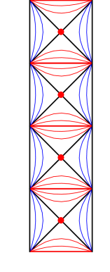
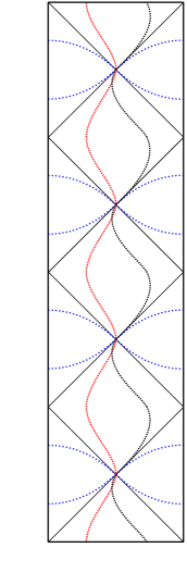
Figure 1: Conjugacy classes and exponential curves in $\widetilde{\mathrm{SU}}(1,1)$. The diagram on the left shows selected conjugacy classes from the list (4.3), including single element (red dots), elliptic (red), parabolic (black) and hyperbolic conjugacy classes (blue). The diagram on the right shows selected exponential curves (4.51) with initial tangent vector $p$ timelike (red), lightlike (black) and spacelike (blue).

The decomposition (4.41) can be be visualised and illustrated by thinking of $\widetilde{\mathrm{SU}}(1,1)$ as an infinite cylinder, with $\omega$ plotted along the vertical axis and $\gamma$ parametrising the horizontal slices. In Fig. 1 we show a vertical cross section of this cylinder and display the conjugacy classes and the exponential curves.

A full list of conjugacy classes of $\widetilde{\mathrm{SU}}(1,1)$ is given in the appendix of [22]. There are four kinds: single element conjugacy consisting of the elements $\Omega^{n}$, as well as elliptic, parabolic and hyperbolic conjugacy classes covering the corresponding classification for $\mathrm{SU}(1,1)$ discussed in Sect. 2. In terms of the decomposition (4.41), they can be described as follows:

$$O^{n} =\{\widetilde{\exp}(p)\Omega^{n}\in\widetilde{\mathrm{SU}}(1,1)|p=0\},$$

$$E^{n}_{\mu_{0}} =\{\widetilde{\exp}(p)\Omega^{n}\in\widetilde{\mathrm{SU}}(1,1)|p^{0}>0,\lambda|{\mbox{\boldmath$p$}}|=\mu_{0},0<\mu_{0}<2\pi\},=E(\mu_{0}+2\pi n)$$

$$P^{n}_{+} =\{\widetilde{\exp}(p)\Omega^{n}\in\widetilde{\mathrm{SU}}(1,1)|p^{0}>0,{\mbox{\boldmath$p$}}^{2}=0\},$$

$$P^{n}_{-} =\{\widetilde{\exp}(p)\Omega^{n}\in\widetilde{\mathrm{SU}}(1,1)|p^{0}<0,{\mbox{\boldmath$p$}}^{2}=0\},$$

$$H^{n}_{\xi} =\{\widetilde{\exp}(p)\Omega^{n}\in\widetilde{\mathrm{SU}}(1,1)|{\mbox{\boldmath$p$}}^{2}=-\xi^{2}<0\}.$$ (4.50)

The diagram on the right in Fig. 1 shows schematic sketches of exponential curves of the form

$$\Gamma_{p,n}=\{\widetilde{\exp}(tp)\Omega^{n}|t\in[0,\infty)]\},$$ (4.51)

where $p$ is a fixed element of $\mathfrak{su}(1,1)$, and $n\in\mathbb{Z}$. In other words, these are images of the exponential map with chosen initial tangent vector $p$ translated by $\Omega^{n}$. We stress that the cross section we are showing suppresses the three-dimensional nature of these curves. To illustrate this, we show three-dimensional plots of some exponential curves starting at the identity in Fig. 2. Note that the spacelike and lightlike curves approach the boundary of the cylinder, but that the timelike curve winds round the axis of the cylinder, carrying out a complete rotation when $\omega$ increases by $2\pi$

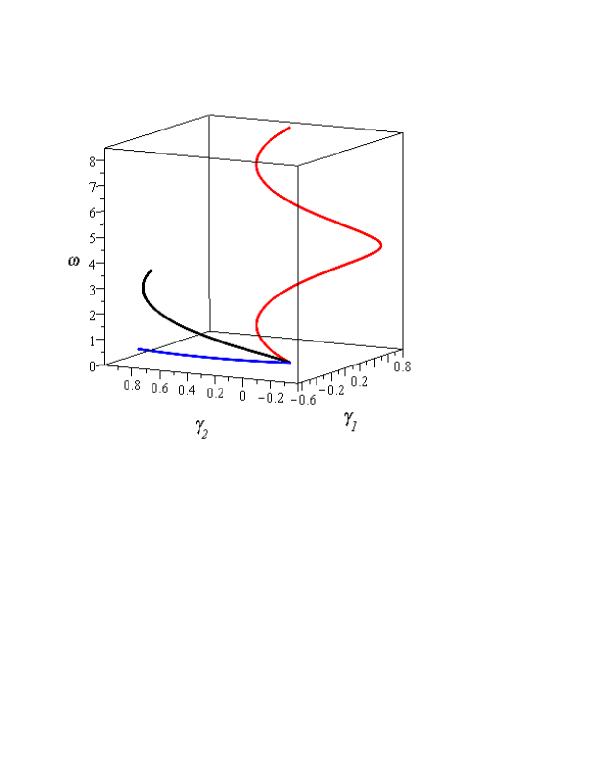
Figure 2: Exponential curves in $\widetilde{\mathrm{SU}}(1,1)$, obtained by exponentiating a spacelike (blue), lightlike (black) and timelike (red) tangent vector at the identity.

In order to compute the group Fourier transform we require an expression for the Haar measure on $\widetilde{\mathrm{SU}}(1,1)$ in the coordinates (4.41). Using the abbreviations introduced in (2.25), we note that for $u=\exp(p)$, the left-invariant Maurer-Cartan form is

$$u^{-1}\mathrm{d}u=\lambda\mathrm{d}|{\mbox{\boldmath$p$}}|\hat{p}\cdot{\mbox{\boldmath$s$}}-2cs\,\mathrm{d}\hat{p}\cdot{\mbox{\boldmath$s$}}-2s^{2}\hat{p}\times\mathrm{d}\hat{p}\cdot{s},$$ (4.52)

where we use (2.28) and suppressed the argument $|{\mbox{\boldmath$p$}}|$ of the functions $c$ and $s$ for readability. Thus

$$[u^{-1}\mathrm{d}u,u^{-1}\mathrm{d}u]=4s^{2}\mathrm{d}\hat{p}\times\mathrm{d}\hat{p}\cdot{\mbox{\boldmath$s$}}-4\lambda cs\,\mathrm{d}|{\mbox{\boldmath$p$}}|\wedge(\hat{p}\times\mathrm{d}\hat{p})\cdot{\mbox{\boldmath$s$}}+4\hat{p}^{2}\lambda s^{2}\mathrm{d}|{\mbox{\boldmath$p$}}|\wedge\mathrm{d}\hat{p}\cdot{\mbox{\boldmath$s$}}.$$ (4.53)

Thus, multiplying out and using again (2.28), the Haar measure in exponential coordinates comes out as

$$du =\mathrm{tr}\left(u^{-1}\mathrm{d}u\wedge u^{-1}\mathrm{d}u\wedge u^{-1}\mathrm{d}u\right)$$

$$=\frac{1}{2}\mathrm{tr}\left([u^{-1}\mathrm{d}u,u^{-1}\mathrm{d}u]\wedge u^{-1}\mathrm{d}u\right)$$

$$=6\lambda s^{2}\,\mathrm{d}\hat{p}\times\mathrm{d}\hat{p}\cdot\hat{p}\wedge\mathrm{d}|{\mbox{\boldmath$p$}}|.$$ (4.54)

Away from the set of measure zero where ${\mbox{\boldmath$p$}}^{2}=0$, we have

$$d^{3}{\mbox{\boldmath$p$}}=\mathrm{d}p^{0}\wedge\mathrm{d}p^{1}\wedge\mathrm{d}p^{2}=\frac{1}{6}\mathrm{d}{\mbox{\boldmath$p$}}\times\mathrm{d}{\mbox{\boldmath$p$}}\cdot\mathrm{d}{\mbox{\boldmath$p$}}=\frac{1}{2}|{\mbox{\boldmath$p$}}|^{2}\mathrm{d}\hat{p}\times\mathrm{d}\hat{p}\cdot\hat{p}\wedge\mathrm{d}|{\mbox{\boldmath$p$}}|,$$ (4.55)

so that, again away from the set where ${\mbox{\boldmath$p$}}^{2}=0$,

$$du=\rho(p)d^{3}{\mbox{\boldmath$p$}},\quad\text{with}\quad\rho(p)=12\lambda\frac{s^{2}(|{\mbox{\boldmath$p$}}|)}{|{\mbox{\boldmath$p$}}|^{2}}.$$ (4.56)

Our parametrisation (4.41) of elements in $\widetilde{\mathrm{SU}}(1,1)$ requires both an element $p\in\mathfrak{su}(1,1)$ and an integer $n$. It is clear that a suitable non-commutative wave cannot depend only on a dual variable $x\in\mathfrak{su}(1,1)^{*}$. It also requires an argument which is dual to the integer $n$. The most natural candidate is an angular coordinate, parametrising a circle $S^{1}$. The necessity of a fourth and circular dimension to describe the spacetime dual to $\widetilde{\mathrm{SU}}(1,1)$ is a surprise. We will introduce it and explore its consequences at this point, postponing a discussion to our final section.

Definition 4.6.

We define non-commutative plane waves for $\widetilde{\mathrm{SU}}(1,1)$ as the maps

$$E:\widetilde{\mathrm{SU}}(1,1)\times(\mathfrak{su}(1,1)^{*}\times S^{1}) \rightarrow\mathbb{C},$$

$$E(u;x,\varphi)=\frac{1}{\rho(p)}e^{i(\langle x,p\rangle+n\varphi)},$$ (4.57)

where $p\in\mathfrak{su}(1,1)$ and $n\in\mathbb{Z}$ are the parameters determining $u$ via the decomposition (4.41), and $\varphi\in[0,2\pi)$ is an angular coordinate on the circle $S^{1}$.

We need to check that the non-commutative waves satisfy a suitable version of the completeness relation (4.2). Expressing the $\delta$-function with respect to the left Haar measure on $\widetilde{\mathrm{SU}}(1,1)$ in terms of the parameters $p$ and $n$ (see also B in [7]),

$$\delta_{e}(g)=\frac{\delta_{n,0}}{\rho(p)}\delta^{3}({\mbox{\boldmath$p$}}),$$ (4.58)

we confirm the required condition:

$$\frac{1}{(2\pi)^{4}}\int_{\mathfrak{su}(1,1)^{*}\times S^{1}}E(u;x,\varphi)\;dxd\varphi =\frac{1}{2\pi}\int_{S^{1}}e^{in\varphi}\,d\varphi\;\frac{1}{(2\pi)^{3}}\int_{\mathbb{R}^{3}}\,\frac{1}{\rho(p)}e^{i{\mbox{\boldmath$p$}}\cdot{\mbox{\boldmath$x$}}}\,d^{3}{\mbox{\boldmath$x$}}$$

$$=\delta_{n,0}\,\frac{1}{\rho(p)}\delta^{3}({\mbox{\boldmath$p$}})$$

$$=\delta_{e}(u).$$ (4.59)

Before we use our non-commutative waves to carry out the group Fourier transform, we make some observations and comments. With the terminology explained after (3.23), the non-commutative waves

$$e^{i(\langle x,p\rangle+n\varphi)}=e^{i({\mbox{\boldmath$x$}}\cdot{\mbox{\boldmath$p$}}+n\varphi)}$$ (4.60)

look like standard plane waves on the product of Minkowski space with a circle. However, the momentum $p$ is constrained by the conditions in (4.41), so that timelike momenta have an invariant mass which is bounded from above by

$$m_{p}=\frac{2\pi}{\lambda}=\frac{1}{4G},$$ (4.61)

and are always in the forward lightcone. The existence of the Lorentz-invariant Planck mass $m_{p}$, and hence also of an invariant Planck length, in the Lorentz double is one of its important features. It means in particular that it provides an example of a ‘doubly special theory of relativity’ in 2+1 dimensions which neither deforms nor breaks Lorentz symmetry, see [27] and our Summary and Outlook for further comments on this point.

It is natural to interpret the integer $n$ in the spirit of particle physics as a label for different kinds of particles in the theory. Timelike momenta $p$ with $n=-1$ may then be viewed as describing antiparticles. Lightlike and spacelike momenta for $n=0$ have the usual interpretation as momenta of massless or (hypothetical) tachyonic particles. The other values of $n$ describe additional types of massive, massless and tachyonic particles. Their existence is required by the fusion rules obeyed by the plane waves, which follow from the star product

$$e^{i(\langle x,p_{1}\rangle+n_{1}\varphi)}\star e^{i(\langle x,p_{2}\rangle+n_{2}\varphi)}=e^{i(\langle x,p(u_{1}u_{2})\rangle+n(u_{1}u_{2})\varphi)}.$$ (4.62)

The general features of this fusion rule can be read off from the picture of the conjugacy classes of $\widetilde{\mathrm{SU}}(1,1)$ on the left in Fig. 1. When multiplying plane waves for particles of types $n_{1}$ and $n_{2}$, the particle type of the combined system is determined by the product, in $\widetilde{\mathrm{SU}}(1,1)$, of the group-valued momenta $u_{1}$ and $u_{2}$. This is a generalisation of the well-know Gott-pair in 2+1 gravity, where two ordinary particles ($n=0$) with high relative speed can combine into a particle with tachyonic momentum (and, in our terminology, of type $n=1$).

Thus we think of the plane waves for $\widetilde{\mathrm{SU}}(1,1)$ as describing kinematic states of particles in a theory with an invariant mass scale $m_{p}$ and with infinitely many different types of particles which combine according to the fusion rules encoded in the star product.

The Fourier transform of a covariant field $\tilde{\phi}:\widetilde{\mathrm{SU}}(1,1)\rightarrow\mathcal{H}_{l\pm}$ is given by

$$\phi(x,\varphi)=\int E(u;x,\varphi)\tilde{\phi}(u)\,du=\sum_{n\in\mathbb{Z}}\int_{B_{+}}e^{i(\langle x,p\rangle+n\varphi)}\tilde{\phi}(u)\,d^{3}{\mbox{\boldmath$p$}},$$ (4.63)

where

$$B_{+}=\{p=-\lambda{\mbox{\boldmath$p$}}\cdot{\mbox{\boldmath$s$}}\in\mathfrak{su}(1,1)|\lambda^{2}{\mbox{\boldmath$p$}}^{2}<(2\pi)^{2},p^{0}>0\;\;\text{if}\;{\mbox{\boldmath$p$}}^{2}>0\}$$ (4.64)

is the region in momentum space required in the parametrisation (4.41).

Since the field $\phi$ takes values in the Hilbert space $\mathcal{H}_{l\pm}$, the extension of the $\star$-product (4.62) to products of such fields requires a careful tensor product decomposition. We will not pursue this here, but note that the decomposition of tensor products in the equivariant formulation of the UIRs for quantum doubles of compact Lie groups was studied in detail in [33]. A full study of the $\star$-product for covariant fields $\phi$ will require an extension to non-compact groups and an adaptation of the results of that paper to our covariant formulation.

Here, we focus on single fields and apply the group Fourier transform to the deformed anyonic spin constraint (4.20) and the mass constraints (4.24) and (4.25). Expanding $u\in\mathrm{SU}(1,1)$ as in (4.41), we first note that

$$D_{l\pm}(u)=D_{l\pm}(\Omega^{n}\widetilde{\exp}(p))=e^{2\pi ins}D_{l\pm}(\widetilde{\exp}(p))=e^{2\pi ins}e^{d_{l\pm}(p)}.$$ (4.65)

But then, with $\lambda m=\mu$ and the decomposition (4.9), we also have

$$e^{i\lambda ms}=e^{i\mu_{0}s}e^{2\pi ins}.$$ (4.66)

Hence, with $p=-\lambda s^{a}p_{a}$, the momentum space spin constraint (4.20) is equivalent to

$$\left(e^{-\lambda d_{l\pm}(s^{a})p_{a}}-e^{i\mu_{0}s}\right)\tilde{\phi}_{\pm}(u)=0.$$ (4.67)

The mass constraints (4.24) and (4.25) also take a simple form in the parametrisation (4.41). The former only see the fractional part $\mu_{0}\in(0,2\pi)$ of $\lambda m$, and is equivalent to

$${\mbox{\boldmath$p$}}^{2}=\frac{\mu_{0}^{2}}{\lambda^{2}}.$$ (4.68)

The condition (4.25) simply fixes the integer $n$ in the decomposition (4.41).

Applying the Fourier transform (4.63) turns the algebraic momentum space constraints into differential equations. The mass constraint (4.68) becomes the Klein-Gordon equation for the fractional part of the mass:

$$\left((\partial_{0}^{2}-\partial_{1}^{2}-\partial_{2}^{2})+\frac{\mu_{0}^{2}}{\lambda^{2}}\right)\phi(x,\varphi)=0.$$ (4.69)

The integer constraint (4.25) fixes the integer part of the mass via the differential condition on the angular dependence of $\phi$:

$$-i\frac{\partial}{\partial\varphi}\phi(x,\varphi)=n\phi(x,\varphi).$$ (4.70)

Finally, the spin constraint (4.67) becomes

$$\left(e^{i\lambda d_{l\pm}(s^{a})\partial_{a}}-e^{i\mu_{0}s}\right)\phi_{\pm}(x,\varphi)=0.$$ (4.71)

This equation involves an exponential of the differential operators (3.29)and (3.30), combining spacetime derivatives with complex derivatives in the hyperbolic disk. This is the anyonic generalisation of the exponential Dirac operator $e^{-\frac{\lambda}{2}\gamma^{a}\partial_{a}}\phi(x)$ that was obtained in [3] for the massive spin $\frac{1}{2}$ particle.

Similar exponential operators have been considered in a more general context in [34], where it was stressed that they are essentially finite difference operators. The appearance of difference-differential equations was first mentioned in relation to (2+1) gravity in [35].

It is clear that further work is required to make sense of the equation (4.71). Stripped down to its simplest elements (by reducing all dimensions to one), it is an equation of the form

$$e^{\lambda\frac{\mathrm{d}}{\mathrm{d}x}}\phi(x)=e^{\lambda k}\phi(x),$$ (4.72)

or, assuming analyticity,

$$\phi(x+\lambda)=e^{\lambda k}\phi(x).$$ (4.73)

For analytic functions, this is equivalent to the infinitesimal version

$$\frac{\mathrm{d}\phi}{\mathrm{d}x}=k\phi(x),$$ (4.74)

obtained by differentiating with respect to $\lambda$. This simple example suggests that the anyonic constraint (3.27) and the gravitational anyonic constrained (4.71) may, suitably defined, be infinitesimal and finite versions of the same condition. However, careful analysis is required to clarify the definition of (4.71) and its relation to (3.27).

5 Summary and Outlook

This paper was motivated by the observation that, in the context of 2+1 dimensional quantum gravity, the spin quantisation (1.1) forces one to consider the universal cover of the Lorentz group and that, in order to preserve the duality between momentum space and Lorentz transformations in the quantum double, it is natural to take the universal cover in momentum space, too.

We showed how the representation theory of the quantum double of the universal cover $\widetilde{\mathrm{SU}}(1,1)$ can be cast in a Lorentz-covariant form, and can be Fourier transformed. In this process, the universal covering of the Lorentz group necessitates the use of infinite-component fields, but the universal covering of momentum space has more interesting and far-reaching consequences.

The first of these, exhibited both in the decomposition (4.9) and in the parametrisation (4.41), is the extension of the range of the allowed mass. The fractional part $\mu_{0}$ of $\mu=8\pi Gm$ is the conventional mass of a particle, which manifests itself in classical (2+1)-dimensional gravity as a conical deficit angle in the spacetime surrounding the particle. The integer label $n$ in the decomposition $\mu=\mu_{0}+2\pi n$ appears to be a purely quantum observable with no classical analogue. It manifests itself, for example, in the Aharonov-Bohm scattering cross section of two massive particles, as discussed in [22]. It is a rather striking illustration of the concept of ‘quantum modular observables’ as introduced in [36], extensively discussed in the textbook [37] and recently applied to the notion of spacetime in [38].

We have chosen to interpret $n$ as a label of different types of particles or matter in (2+1)-dimensional quantum gravity. These particles can be converted into each other during interactions, according to fusion rules determined by the group product in $\widetilde{\mathrm{SU}}(1,1)$ and the decomposition of factors and products according (4.41).

The second and surprising consequence of the universal covering of momentum space is the appearance of an additional and compact dimension on the dual side, in spacetime. This is needed to define the group Fourier transform, and allows for a simple expression of the constraint determining the particle type $n$ as a differential condition.

Our results raise a number of questions and suggest avenues for future research. As discussed at the end of the previous section, the exponentiated differential operators which generically appear as group Fourier transforms of the spin constraint should be studied using rigorous analysis. One expects these to be natural operators, possibly best defined as difference operators, not least because they are, by Lemma 4.3, essentially Fourier transforms of the ribbon element of the quantum double.

It seems clear that our Hilbert-space valued fields $\phi$ on Minkowski space equipped with a $\star$-product fit rather naturally into the framework of braided quantum field theories, defined in [39] and studied, in a Euclidean setting, in [4, 40]. Our paper is only concerned with a single particle and we only looked at simple examples of fusion rules for two spinless particles. However, braided quantum field theory naturally provides the language for discussing the gravitational interactions of several gravitational anyons in a spacetime setting. This provides an alternative viewpoint to existing momentum space discussions, with the non-commutative $\star$-product and the universal $R$-matrix of the quantum double encoding the quantum-gravitational interactions.

It is worth stressing that the $\star$-product on Minkowski space considered here preserves Lorentz covariance, and that any braided quantum field theory constructed from it would similarly be Lorentz covariant. This follows essentially from the Lorentz invariance of the mass scale (4.61) and the associated Planck length scale [28]. It reflects the important fact that the Lorentz double deforms Poincaré symmetry by introducing a mass scale while preserving Lorentz symmetry, which is a challenge for any theory of quantum gravity.

Finally, it would be interesting to repeat the analysis of this paper with the inclusion of a cosmological constant. This leads to a $q$-deformation of the quantum double of $\widetilde{\mathrm{SU}}(1,1)$ [28], and there should similarly be a $q$-deformation of the spacetime picture of the representations. Some remarks on how this might work are made in [2], but none of the details have been worked out. In the Lorentzian context, a positive cosmological constant will lead to real deformation parameter $q$ while a negative cosmological constant will lead to $q$ lying on the unit circle [28]. It would clearly be interesting to understand how this change in $q$ captures the radically different physics of the two regimes.

Acknowledgements   SI acknowledges support through an EPSRC doctoral training grant. Several of the results in this paper were reported by BJS at the Workshop on Quantum Groups in Quantum Gravity, University of Waterloo 2016. BJS thanks the organisers for the invitation, and acknowledges discussions with participants at the workshop. We thank Peter Horvathy for drawing our attention to Plyushchay’s work on anyonic wave equations and to their joint work on noncommutative waves.

References

- [1] A. Khare, Fractional statistics and quantum theory, 2nd edition, World Scientific, Singapore, 2005.
- [2] S. Majid and B. J. Schroers, -Deformation and semidualisation in 3D quantum gravity, J. Phys. A 42 (2009) 425402.
- [3] B. J. Schroers and M. Wilhelm, Towards non-commutative deformations of relativistic wave equations in 2+1 dimensions, SIGMA 10 (2014) 053.
- [4] L. Freidel and E. R. Livine, Effective 3-D quantum gravity and non-commutative quantum field theory, Phys. Rev. Lett. 96 (2006) 221301.
- [5] L. Freidel and S. Majid, Noncommutative harmonic analysis, sampling theory and the Duflo map in 2+1 quantum gravity, Class. Quant. Grav. 25 (2008) 045006.
- [6] M. Raasakka, Group Fourier transform and the phase space path integral for finite dimensional Lie groups, arXiv:1111.6481.
- [7] C. Guedes, D. Oriti, M. Raasakka, Quantization maps, algebra representation, and non-commutative Fourier transform for Lie groups, J. Math. Phys. 54 (2013) 083508.
- [8] M. A. Rieffel, Lie group convolution algebras as deformation quantizations of linear Poisson structures, Am. J. Mathematics 112 (1990) 657–685.
- [9] E. P. Wigner On unitary representations of the inhomogeneous Lorentz group, Annals of Mathematics 40 (1939) 149–204.
- [10] D. R. Grigore, The projective unitary representations of the Poincaré group in 1+2 dimensions, J. Math. Phys. 34 (1993) 4172–4189.
- [11] B. Binegar, Relativistic field theories in three dimensions, J. Math. Phys. 23 (8) (1982) 1511–1517.
- [12] D. M. Gitman and A. L. Shelepin, Poincaré group and relativistic wave equation in 2+1 dimensions, J. Phys. A: Math. Gen. 30 (1997) 6093–6121.
- [13] R. Jackiw and V. P. Nair, Relativistic wave equations for anyons, Phys. Rev. D43 (1991) 1933–1942.
- [14] M. S. Plyushchay, Relativistic particle with torsion, Majorana equation and fractional spin, Phys. Lett. B 262 (1991) 71–78.
- [15] M. S. Plyushchay, The model of the relativistic particle with torsion, Nucl. Phys. B362 (1991) 54–72.
- [16] E. Majorana, Teoria relativistica di particelle con momento intrinseco arbitrario, Nuovo Cimento 9 (1932) 335–344.
- [17] D. Tz. Stoyanov and I. T. Todorov, Majorana representations of the Lorentz group and infinite-component fields, J. Math. Phys. 9 (1968) 2146–2167.
- [18] C. Meusburger and B. J. Schroers, Poisson structure and symmetry in the Chern-Simons formulation of (2+1)-dimensional gravity, Class. Quant. Grav. 20 (2003) 2193–2233.
- [19] C. Meusburger and B. J. Schroers, The quantisation of Poisson structures arising in Chern-Simons theory with gauge group , Adv. Theor. Math. Phys. 7 (2004) 1003–1043.
- [20] C. Meusburger and K. Noui, The Hilbert space of 3d gravity: quantum group symmetries and observables, Adv. Theor. Math. Phys. 14 (2010), 1651–1716.
- [21] B. J. Schroers, Combinatorial quantisation of Euclidean gravity in three dimensions, in N. P. Landsman et al Quantization of singular symplectic quotients, Progress in Mathematics, Vol. 198 (2001) 307–328.
- [22] F. A. Bais and N. M. Muller, B. J. Schroers, Quantum group symmetry and particle scattering in (2+1)-dimensional quantum gravity, Nucl. Phys. B640 (2002) 3–45.
- [23] J. Louko and H. J. Matschull The 2+1 Kepler problem and its quantization, Class. Quant. Grav. 18 (2001) 2731–2784.
- [24] P. A. Horváthy and M. S. Plyushchay, Anyon wave equations and the non-commutative plane, Phys. Lett. B 595 (2004) 547–555.
- [25] P. J. Sally Jr, Analytic continuation of the irreducible unitary representations of the universal covering group of , Memoirs of the American Mathematical Society Number 69, 1967.
- [26] A. O. Barut and R. Raczka, Theory of group representations and applications, World Scientific, Singapore, 1986.
- [27] B. J. Schroers, Lessons from 2+1 dimensional quantum gravity, PoS QG-PH (2007) 035.
- [28] B. J. Schroers, Quantum gravity and non-commutative spacetimes in three dimensions: a unified approach, Acta Phys. Polon. Supp. 4 (2011) 379–402.
- [29] G. ’t Hooft, Non-perturbative 2-particle scattering amplitude in 2+1 dimensional quantum gravity, Commun. Math. Phys. 117 (1988) 685–700.
- [30] S. Deser and R. Jackiw, Classical and quantum scattering on a cone, Commun. Math. Phys. 118 (1988) 495–509.
- [31] F. A. Bais and N. M. Muller, Topological field theory and the quantum double of SU(2), Nucl. Phys. B530 (1998) 349–400.
- [32] T. H. Koornwinder and N. M. Muller, The quantum double of a (locally) compact group, J. Lie Theory 7 (1997),101–120.
- [33] T. H. Koornwinder, F. A. Bais and N. M. Muller, Tensor product representations of the quantum double of a compact group, Commun. Math. Phys. 198 (1998) 157–186.
- [34] M. F. Atiyah and G. W. Moore, A shifted view of fundamental physics, arXiv:1009.3176.
- [35] H. J. Matschull and M. Welling, Quantum mechanics of a point particle in 2+1 dimensional gravity, Class. Quant. Grav. 15 (1998) 2981–3030.
- [36] Y. Aharonov, H. Pendleton and A. Petersen, Modular variables in quantum theory, Int. Jour. Theor. Phys. 2 (1969) 213.
- [37] Y. Aharonov and D. Rohrlich, Quantum paradoxes: quantum theory for the perplexed, Wiley VCH, 2005.
- [38] L. Freidel, R. G. Leigh, D. Minic, Quantum spaces are modular, Phys. Rev. D94 (2016) 104052.
- [39] R. Oeckl, Introduction to braided quantum field theory, Int. J. Mod. Phys. B14 (2000) 2461–2466.
- [40] Y. Sasai and N. Sasakura, Braided quantum field theories and their symmetries, Prog. Theor. Phys. 118 (2007) 785–814.