SMA observations of the polarized dust emission in solar-type Class 0 protostars: the magnetic field properties at envelope scales

Abstract

Aims. Although, from a theoretical point of view, magnetic fields are believed to have a significant role during the early stages of star formation, especially during the main accretion phase, the magnetic field strength and topology is poorly constrained in the youngest accreting Class 0 protostars that lead to the formation of solar-type stars.

Methods. We carried out observations of the polarized dust continuum emission with the SMA interferometer at 0.87mm, in order to probe the structure of the magnetic field in a sample of 12 low-mass Class 0 envelopes, including both single protostars and multiple systems, in nearby clouds. Our SMA observations probe the envelope emission at scales $\sim 600-5000$ au with a spatial resolution ranging from 600 to 1500 au depending on the source distance.

Results. We report the detection of linearly polarized dust continuum emission in all of our targets, with average polarization fractions ranging from 2% to 10% in these protostellar envelopes. The polarization fraction decreases with the continuum flux density, which translates into a decrease with the H₂ column density within an individual envelope. Our analysis show that the envelope-scale magnetic field is preferentially observed either aligned or perpendicular to the outflow direction. Interestingly, our results suggest for the first time a relation between the orientation of the magnetic field and the rotational energy of envelopes, with a larger occurrence of misalignment in sources where strong rotational motions are detected at hundreds to thousands of au scales. We also show that the best agreement between the magnetic field and outflow orientation is found in sources showing no small-scale multiplicity and no large disks at $\sim$100 au scales.

1 Introduction

Understanding the physical processes at work during the earliest phase of star formation is key to characterize the typical outcome of the star formation process, put constraints on the efficiency of the accretion/ejection mechanisms and determine the pristine properties of the planet-forming material. Class 0 objects are the youngest accreting protostars (Andre et al., 1993, 2000): the bulk of their mass resides in a dense envelope that is being actively accreted onto the central protostellar embryo, during a short main accretion phase (t $<10^{5}$ yr, Maury et al. 2011; Evans et al. 2009). The physics at work to reconcile the order-of-magnitude difference between the large angular momentum of prestellar cores (Goodman et al., 1993; Caselli et al., 2002) and the rotation properties of the young main sequence stars (also called the “angular momentum problem”; Bodenheimer, 1995; Belloche, 2013) is still not fully understood. It was proposed that the angular momentum could be strongly reduced by the fragmentation of the core in multiple systems, or the formation of a protostellar disk and/or launch of a jet carrying away angular momentum. None of these solutions, however, seems to be able to reduce the angular momentum of the core’s material by the required 5 to 10 orders of magnitude.

Magnetized models have shown that the outcome of the collapse phase can be significantly modified through ‘magnetic braking’ (Galli et al., 2006; Li et al., 2014). The role of magnetic fields on Class 0 properties have also been investigated observationally. A few studies have been comparing the observations of Class 0 protostars to the outcome of models, either analytically (see e.g. Frau et al., 2011) or from magneto-hydrodynamical simulations (see e.g. Maury et al., 2010, 2018). They showed that magnetized models of protostellar formation better reproduce the observed small-scale properties of the youngest accreting protostars, for instance the lack of fragmentation and the paucity of large (100 $<$ r_disk $<$ 500 au) rotationally-supported disks (Maury et al., 2010; Enoch et al., 2011; Maury et al., 2014; Segura-Cox et al., 2016) observed in Class 0 objects.

The polarization of the thermal dust continuum emission provides an indirect probe of the magnetic field topology since the long axis of non-spherical or irregular dust grains is suggested to align perpendicular to the magnetic field direction (Lazarian, 2007). Recently, the Planck Space Observatory produced an all-sky map of the polarized dust emission at sub-millimeter (submm) wavelengths, revealing that the Galactic magnetic field shows regular patterns (Planck Collaboration, 2016). Observations at better angular resolution obtained from ground-based facilities seem to indicate that the polarization patterns are well ordered at the scale of Hii regions or molecular cloud complexes (Curran & Chrysostomou, 2007; Matthews et al., 2009; Poidevin et al., 2010). We refer the reader to Crutcher (2012) and references therein for a review on magnetic fields in molecular clouds.

Few polarization observations have been performed to characterize the magnetic field topology at the protostellar envelope scales where the angular momentum problem is relevant. Submm interferometric observations of the polarized dust continuum emission with the SMA (Submillimeter Array; Ho et al., 2004) and CARMA (Combined Array for Research in Millimeter-wave Astronomy; Bock et al., 2006) interferometers have led to the detections of polarized dust continuum emission toward a dozen of low-mass Class 0 protostars (Rao et al., 2009; Girart et al., 2006; Hull et al., 2014), in particular luminous and/or massive objects because of the strong sensitivity limitations to detect a few percent of the dust continuum emission emitted by low-mass objects. By comparing the large ($\sim$20″) and small ($\sim$2.5″) scale B fields of protostars at 1mm (TADPOL survey), Hull et al. (2014) find that sources in which the large and small magnetic field orientations are consistent tend to have higher fractional polarization, which could be a sign of the ‘regulating’ role of magnetic fields during the infall of the protostellar core. No systematic relation, however, seems to exist between the core magnetic field direction and the outflow orientation (Curran & Chrysostomou, 2007; Hull et al., 2013; Zhang et al., 2014). An hourglass shape of the magnetic line segments was observed in several protostellar cores (Girart et al., 1999; Lai et al., 2002; Girart et al., 2006; Rao et al., 2009; Stephens et al., 2013). Probably linked with the envelope contraction pulling the magnetic field lines toward the central potential well, this hourglass pattern could depend strongly on the alignment between the core rotation axis and the magnetic field direction (Kataoka et al., 2012). ALMA observations are now pushing the resolution and sensitivity enough to be probing down to 100 au scales in closeby low-mass Class 0 protostars. In the massive ($M_{\textrm{env}}$$\sim$20 $M_{\odot}$) binary protostar Serpens SMM1, they have revealed a chaotic magnetic field morphology affected by the outflow (Hull et al., 2017). In the solar-type Class 0 B335, they have, on the contrary, unveiled very ordered topologies, with a clear transition from a large-scale B-field parallel to the outflow direction to a strongly pinched B in the equatorial plane (Maury et al., 2018).

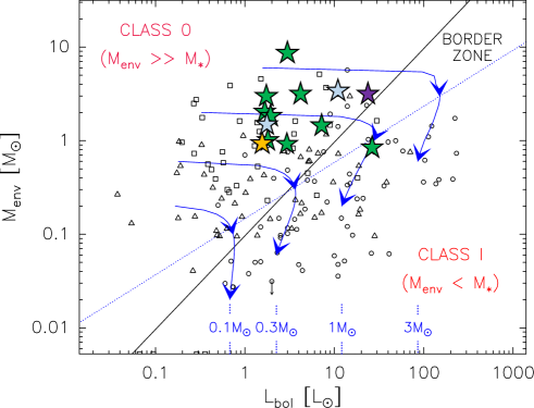
Figure 1: Envelope mass versus bolometric luminosity diagram from Andre et al. (2000) and Maury et al. (2011). The small black squares and triangles are Class 0 and I protostars detected in the Aquila rift, Ophiuchus, Perseus, and Orion regions (Bontemps et al., 1996; Motte & André, 2001; Andre et al., 2000; Maury et al., 2011; Sadavoy et al., 2014). The lines mark the conceptual border zone between the Class 0 and Class I stage, with $M_{\textrm{env}}$ $\propto$ $L_{\textrm{bol}}$ for the dashed line and $M_{\textrm{env}}$ $\propto$ $L_{\textrm{bol}}^{0.6}$ for the dotted line. Blue lines with arrows represent protostellar evolutionary tracks, computed for final stellar masses of 0.1, 0.3, 1 and 3$M_{\odot}$, with an evolution proceeding from top left (objects with large envelope masses slowly accreting) to bottom (the envelope mass as well as the accretion luminosity are rapidly decreasing). Our sample is overlaid with the positions of protostars in our sample: B335 in yellow, IRAS16293 in purple, Perseus sources in green and Cepheus sources in light blue. It only contains low-mass Class 0 protostars, except for SVS13-A. The $M_{\textrm{env}}$ and $L_{\textrm{bol}}$ are from Massi et al. (2008) for CB230, Launhardt et al. (2013) for B335, Crimier et al. (2010) for IRAS16293, Sadavoy et al. (2014), Ladjelate et al. (in prep.) and Maury et al. (in prep.) for the rest of the sources.

Whether or not magnetic fields play a dominant role in regulating the collapse of protostellar envelopes needs to be further investigated from an observational perspective. In this paper, we analyze observations of the 0.87 mm polarized dust continuum for a sample of 12 Class 0 (single and multiple systems) protostars with the SMA interferometer (Ho et al., 2004) to increase the current statistics on the polarized dust continuum emission detected in protostellar envelopes on 750-2000 au scales. We provide details on the sample and data reduction steps in $\S$2. We study the continuum fluxes and visibility profiles and describe the polarization results in $\S$3. We analyze the polarization fraction dependencies with density and the potential causes of depolarization in $\S$4.1. In $\S$4.2, we analyse the large-to-small-scale B orientation and its variation with wavelength. We finally discuss the relation between the magnetic field orientation and both the rotation and fragmentation properties in the target protostellar envelopes. A summary of this work is presented in $\S$5.

Table 1: Properties of the sample

Name	Cloud	Distance a	Class	Multiplicity b	Observation Phase Reference Center
B335	isolated	100 pc	Class 0	Single	19h37m00.9s  +07$\degr$34$\arcmin$09$\aas@@fstack{\prime\prime}$6
SVS13	Perseus	235 pc	Class 0/I	Multiple (wide)	03h29m03.1s  +31$\degr$15$\arcmin$52$\aas@@fstack{\prime\prime}$0
HH797	Perseus	235 pc	Class 0	Multiple	03h43m57.1s  +32$\degr$03$\arcmin$05$\aas@@fstack{\prime\prime}$6
L1448C	Perseus	235 pc	Class 0	Multiple (wide)	03h25m38.9s  +30$\degr$45$\arcmin$14$\aas@@fstack{\prime\prime}$9
L1448N	Perseus	235 pc	Class 0	Multiple (close and wide)	03h25m36.3s  +30$\degr$44$\arcmin$05$\aas@@fstack{\prime\prime}$4
L1448-2A	Perseus	235 pc	Class 0	Multiple (close and wide)	03h25m22.4s  +30$\degr$45$\arcmin$12$\aas@@fstack{\prime\prime}$2
IRAS03282	Perseus	235 pc	Class 0	Multiple (close)	03h31m20.4s  +30$\degr$45$\arcmin$24$\aas@@fstack{\prime\prime}$7
NGC 1333 IRAS4A	Perseus	235 pc	Class 0	Multiple (close)	03h29m10.5s  +31$\degr$13$\arcmin$31$\aas@@fstack{\prime\prime}$0
NGC 1333 IRAS4B	Perseus	235 pc	Class 0	Single	03h29m12.0s  +31$\degr$13$\arcmin$08$\aas@@fstack{\prime\prime}$0
IRAS16293	Ophiuchus	120 pc	Class 0	Multiple (wide)	16h32m22.9s  -24$\degr$28$\arcmin$36$\aas@@fstack{\prime\prime}$0
L1157	Cepheus	250 pc	Class 0	Single	20h39m06.3s  +68$\degr$02$\arcmin$15$\aas@@fstack{\prime\prime}$8
CB230	Cepheus	325 pc	Class 0	Binary (close)	21h17m40.0s  +68$\degr$17$\arcmin$32$\aas@@fstack{\prime\prime}$0

• Distance references are Knude & Hog (1998), Stutz et al. (2008), Hirota et al. (2008), Hirota et al. (2011), Looney et al. (2007) and Straizys et al. (1992).

• Multiplicity derived from Launhardt (2004) for IRAS03282 and CB230, Rao et al. (2009) for IRAS16293, Palau et al. (2014) for HH797, Evans et al. (2015) for B335 and from the CALYPSO survey dust continuum maps at 220 GHz (PdBI, see http://irfu.cea.fr/Projets/Calypso/), Maury et al. (2014)) for the rest of the sources.

2 Observations and data reduction

2.1 Sample description

Our sample contains 12 protostars that include single objects as well as common-envelope multiple systems and separate envelopes multiple system (Looney et al., 2000, following the classification proposed by). Figure 1 shows the location of the protostars in an envelope mass ($M_{\textrm{env}}$) versus bolometric luminosity ($L_{\mathrm{bol}}$) diagram (Bontemps et al., 1996; Maury et al., 2011). With most of the object mass contained in the envelope, our selection is a robust sample of low-mass Class 0 protostars. Only SVS13-A can be classified as a Class I protostar. Details on each object are provided in Table 1 and in appendix.

2.2 The 0.87mm SMA observations

Observations of the polarized dust emission of 9 low-mass protostars at 0.87mm were obtained using the SMA (Projects 2013A-S034 and 2013B-S027, PI: A. Maury) in the compact and subcompact configuration. To increase our statistics, we also include SMA observations from three additional sources from Perseus (NGC 1333 IRAS4A and IRAS4B) and Ophiuchus (IRAS16293) observed in 2004 and 2006 (Projects 2004-142 and 2006-09-A026, PI: R. Rao; Project 2005-09-S061, PI: D.P. Marrone). The observations of NGC 1333 IRAS4A and IRAS16293 are presented in Girart et al. (2006) and Rao et al. (2009) respectively. We refer the reader to Marrone (2006) and Marrone & Rao (2008) for a detailed description of the SMA polarimeter system, but provide a few details on the SMA and the polarization design here. The SMA has eight antennas. Each optical path is equipped with a quarter-wave plate (QWP), an optical element that adds a 90$\degr$ phase delay between orthogonal linear polarizations and is used to convert the linear into circular polarization. The antennas are switched between polarizations (QWP are rotated at various angles) in a coordinated temporal sequence to sample the various combinations of circular polarizations on each baseline. The 230, 345 and 400 band receivers are installed in all eight SMA antennas. Polarization can be measured in single-receiver polarization mode as well as in dual-receiver mode when two receivers with orthogonal linear polarizations are tuned simultaneously. In this dual-receiver mode, all correlations (the parallel-polarized RR and LL and the cross-polarized RL and LR; with R and L for right circular and left circular respectively) are measured at the same time. Both polarization modes were used in our observations. This campaign was used to partly commission the dual-receiver full polarization mode for the SMA. A fraction of the data was lost during this period due to issues with the correlator software. Frequent observations of various calibrators were interspersed to ensure that such issues were detected as early as possible to minimize data loss.

Table 2: Details on the observations

Date	Mode a	Flux	Bandpass	Gain	Polarization	Antenna
		Calib.	Calib.	Calib.	Calib.	used
Dec 05 2004	Single Rx - Single BW	Ganymede	3c279	3c84	3c279	1, 2, 3, 5, 6, 8
Dec 06 2004	Single Rx - Single BW	Ganymede	3c279	3c84	3c279	1, 2, 3, 5, 6, 8
April 08 2006	Single Rx - Single BW	Callisto	3c273	1517-243, 1622-297	3c273	1, 2, 3, 5, 6, 7, 8
Dec 23 2006	Single Rx - Single BW	Titan	3c279	3c84	3c279	1, 2, 3, 4, 5, 6, 7
Aug 26 2013	Single Rx - Double BW	Neptune	3c84	1927+739, 0102+584	3c84	2, 4, 5, 6, 7, 8
Aug 31 2013	Dual Rx - Autocorrel	Callisto	3c84	1751+096, 1927+739, 0102+584, 3c84	3c84	2, 4, 5, 6, 7, 8
Sept 1 2013	Dual Rx - Autocorrel	Callisto	3c84	1927+739, 0102+584	3c84	2, 4, 5, 6, 7, 8
Sept 2 2013	Dual Rx - Autocorrel	Callisto	3c454.3	1927+739, 0102+584,3c84	3c84	2, 4, 5, 6, 7, 8
Sept 7 2013	Dual Rx - Full pol.	Callisto	3c454.3	3c84, 3c454.3	3c454.3	2, 4, 5, 6, 7, 8
Dec 7 2013	Dual Rx - Full pol.	Callisto	3c84	3c84	3c84	2, 4, 5, 6, 7, 8
Feb 24 2014	Dual Rx - Full pol.	Callisto	3c279	3c84, 3c279, 0927+390	3c279	1, 2, 4, 5, 6, 7
Feb 25 2014	Dual Rx - Full pol.	Callisto	3c84	3c84	3c84	1, 2, 4, 5, 6, 7

• Rx = Receiver; BW = bandwidth.

Table 3: Characteristics of the SMA maps

Name	Synthesized beam			rms (mJy/beam)
				I a	Q	U
B335	4$\aas@@fstack{\prime\prime}$8$\times$4$\aas@@fstack{\prime\prime}$1	(84$\degr$)		4.6	4.0	4.3
SVS13	4$\aas@@fstack{\prime\prime}$9$\times$4$\aas@@fstack{\prime\prime}$3	(-88$\degr$)		7.0	3.0	3.1
HH797	4$\aas@@fstack{\prime\prime}$7$\times$4$\aas@@fstack{\prime\prime}$3	(89$\degr$)		4.2	1.9	1.8
L1448C	4$\aas@@fstack{\prime\prime}$7$\times$4$\aas@@fstack{\prime\prime}$4	(87$\degr$)		4.7	3.6	3.7
L1448N	2$\aas@@fstack{\prime\prime}$6$\times$2$\aas@@fstack{\prime\prime}$4	(55$\degr$)		5.5	3.3	3.0
L1448-2A	2$\aas@@fstack{\prime\prime}$5$\times$2$\aas@@fstack{\prime\prime}$2	(49$\degr$)		1.8	1.6	1.6
IRAS03282	4$\aas@@fstack{\prime\prime}$8$\times$4$\aas@@fstack{\prime\prime}$3	(88$\degr$)		5.3	3.3	3.5
NGC 1333 IRAS4A	2$\aas@@fstack{\prime\prime}$0$\times$1$\aas@@fstack{\prime\prime}$4	(-46$\degr$)		18.7	7.5	8.0
NGC 1333 IRAS4B	2$\aas@@fstack{\prime\prime}$2$\times$1$\aas@@fstack{\prime\prime}$7	(10$\degr$)		9.0	2.2	2.3
IRAS16293	3$\aas@@fstack{\prime\prime}$0$\times$1$\aas@@fstack{\prime\prime}$8	(-6$\degr$)		10.4	5.6	6.0
L1157	5$\aas@@fstack{\prime\prime}$9$\times$4$\aas@@fstack{\prime\prime}$6	(1$\degr$)		8.8	6.4	7.6
CB230	6$\aas@@fstack{\prime\prime}$1$\times$4$\aas@@fstack{\prime\prime}$2	(7$\degr$)		5.5	4.11	4.0

• Stokes I rms noise values reported here come from the maps obtained after self-calibration.

2.3 Data calibration and self-calibration

We perform the data calibration in the IDL-based software MIR (Millimeter Interferometer Reduction) and the data reduction package MIRIAD. The calibration includes: an initial flagging of high system temperatures $T_{\mathrm{sys}}$ and other wrong visibilities, a bandpass calibration, a correction of the cross-receiver delays, a gain and a flux calibration. The various calibrators observed for each of these steps and the list of antennae used for the observations are summarized in Table 2. The polarization calibration was performed in MIRIAD. Quasars were observed to calculate the leakage terms: the leakage amplitudes (accuracy: $\sim$0.5%) are $<$2% in the two sidebands for all antenna except for 7 than can reach a few percent. Before the final imaging, we use an iterative procedure to self-calibrate the Stokes I visibility data.

2.4 Deriving the continuum and polarization maps

The Stokes parameters describing the polarization state are defined as

$$\overrightarrow{S}=\begin{bmatrix}I\\ Q\\ U\\ V\\ \end{bmatrix}$$ (1)

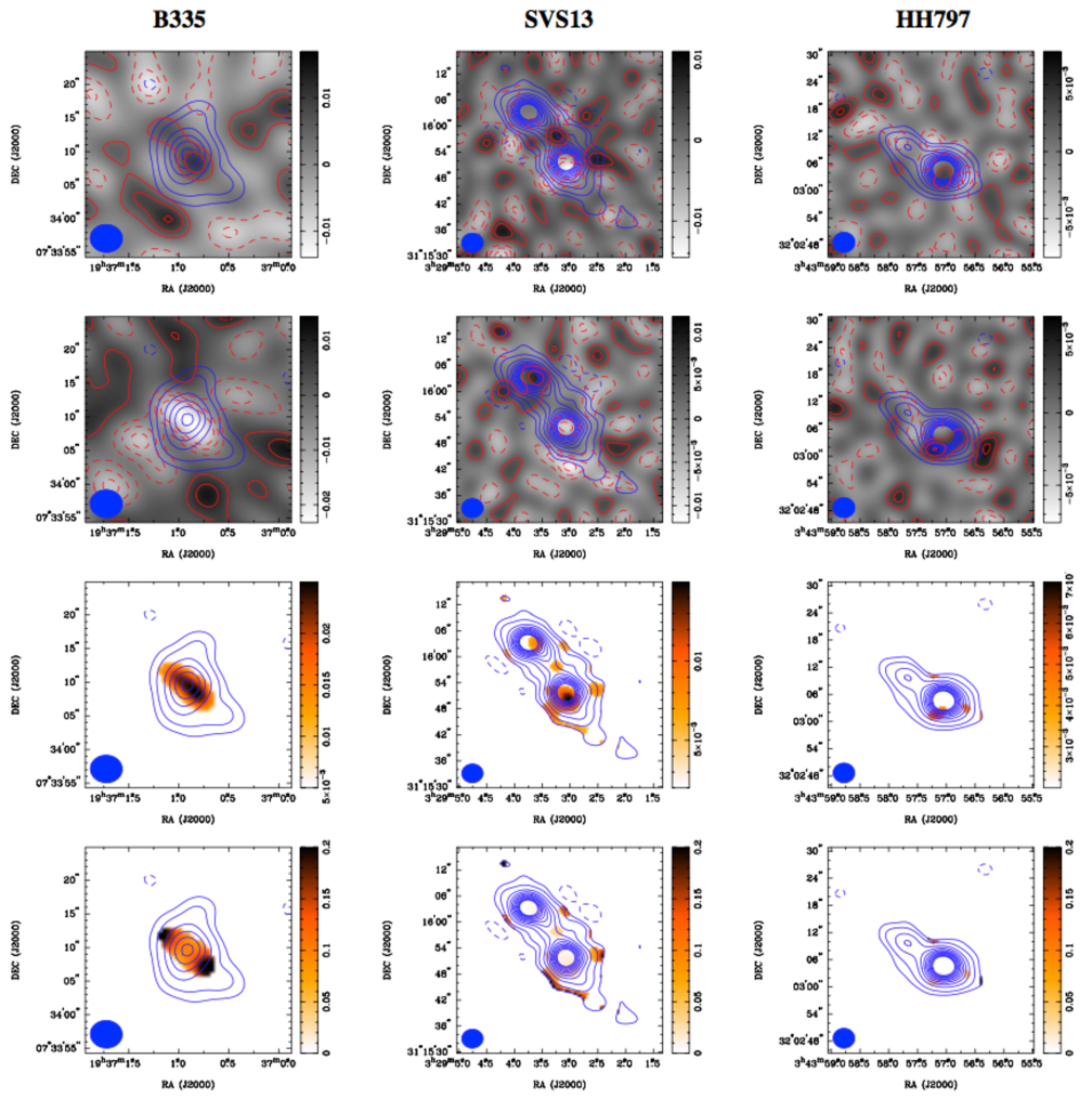
Figure 9: Polarization maps of, from left to right, B335, SVS13 and HH797. Two top panels: Stokes Q and U maps. Color scales are in mJy/beam. Stokes I contours (same as in Fig. 2) appear in blue. Stokes Q and U contours appear in red and are [-3,-2,-1,1,2,3] $\sigma$. Third line: Polarization intensity maps. The color scale is in mJy/beam. Fourth line: Polarization fraction map. The filled ellipses on the lower left corner indicate the synthesized beam of the SMA maps.

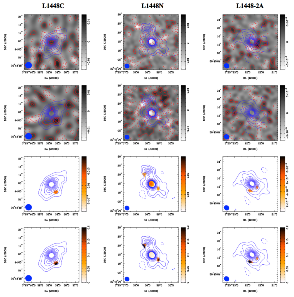
Figure 9: Continued. Same for L1448C, N and 2A.

with Q and U the linear polarization and V the circular polarization. We use a robust weighting of 0.5 to transform the visibility data into a dirty map. The visibilities range from 5 to 30k$\lambda$ in 7 sources (B335, SVS13, HH797, L1448C, IRAS03282, L1157 and CB230) and 10 to 80k$\lambda$ for the other 5 sources. Visibilities beyond 80k$\lambda$ are available for NGC 1333 IRAS4A but not used to allow an analysis of comparable scales for all our sources. The Stokes I dust continuum emission maps are shown in Fig. 2. The Stokes Q and U maps are shown in appendix (Fig. 9). Their combination probes the polarized component of the dust emission. The synthesized beams and rms of the cleaned maps are provided in Table 3. We note that because of unavoidable missing flux and the dynamic-range limitation, the rms of the Stokes I maps are systematically higher than those of Stokes Q and U. Following the self-calibration procedure, the rms of the continuum maps have decreased by 10 to 45%.

The polarization intensity (debiased), fraction and angle are derived from the Stokes Q and U as follow:

$$P_{i}=\sqrt[]{Q^{2}+U^{2}-\sigma_{Q,U}^{2}},\vspace{-2pt}$$ (2)

$$p_{frac}=P_{i}\leavevmode\nobreak\ /\leavevmode\nobreak\ I,\vspace{-2pt}$$ (3)

$$PA=0.5\times\ arctan(U/Q).$$ (4)

with $\sigma$_Q,U the average rms of the Q and U maps. We apply a 5-$\sigma$ cutoff on Stokes I and 3-$\sigma$ cutoff on Stokes Q and U to only select locations where polarized emission is robustly detected. The polarization intensity and fraction maps are provided in appendix (Fig. 9).

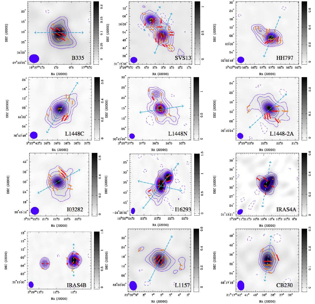
Figure 2: The SMA 850 $\mu$m Stokes I continuum maps. Color scales are in mJy/beam. Contours at [-3,5,10,20,30,40,50,60,70,80,90,100] $\sigma$ appear in blue. The filled ellipses on the lower left corner indicate the synthesized beam of the SMA maps. Their sizes are reported in Table 3. The blue arrows indicate the outflow direction. B orientation (derived from the polarization angles assuming a 90$\degr$ rotation) are overlaid on the Stokes I map. Red bars show $>$3-$\sigma$ detections. We also indicate the $>$2-$\sigma$ detections with orange bars but these detections are not used for this analysis.

Table 4: 0.87mm integrated flux densities, source sizes, polarization intensities and fractions.

Name	On the 0.87mm reconstructed maps						From the visibility amplitude curve
	Flux densitya	Mass	Peak intensity	Peak Pi b	pfrac c		0.87mm Flux density
	(Jy)	($M_{\odot}$)	(Jy/beam)	(mJy/beam)	(%)		(Jy)
B335	0.21$\pm$0.04	0.02	0.24	25.3	10.5		0.51$\pm$0.05
SVS13	1.40$\pm$0.28	0.29	1.06	14.8	2.5		1.54$\pm$0.15d
HH797	0.47$\pm$0.09	0.10	0.71	5.7	3.0		0.94$\pm$0.09
L1448C	0.57$\pm$0.11	0.11	0.65	12.5	-		1.00$\pm$0.01
L1448N	1.50$\pm$0.30	0.31	1.34	20.3	2.7		1.93$\pm$0.19d
L1448-2A	0.34$\pm$0.07	0.07	0.27	5.7	-		0.48$\pm$0.05
IRAS03282	0.44$\pm$0.09	0.09	0.65	9.9	-		1.17$\pm$0.12
NGC 1333 IRAS4A	2.38$\pm$0.48	0.50	2.57	77.3	8.8		6.79$\pm$0.68
NGC 1333 IRAS4B	1.42$\pm$0.28	0.30	2.89	14.9	4.7		4.10$\pm$0.41
IRAS16293	4.81$\pm$0.96	0.26	3.83	39.2	1.7		5.96$\pm$0.60d
L1157	0.43$\pm$0.09	0.10	0.71	31.4	4.5		1.07$\pm$0.11
CB230	0.22$\pm$0.04	0.09	0.37	14.3	6.4		0.58$\pm$0.06

• Flux density estimated within the central 6000 au for SVS13, 3000 au for other sources.

• We remind the reader that not all the sources have an intensity peak co-spatial with the polarized intensity peak.

• Polarization fraction defined as the unweighted ratio between the median polarization over total flux.

• The visibility data allows us to separate the two components of wide binaries. The fluxes reported here are those of the object located at the phase center, e.g. L1448N-B, SVS13-B and IRAS16293-A.

Table 5: Comparison with SCUBA observations from Di Francesco et al. (2008)

Name	SCUBA 850 $\mu$m				Comparison SMA / SCUBA
	Peak Intensity	Effective radius	Flux density		Rescaled Peak Intensitya	Peak intensity Ratio	Total Flux Ratio
	(Jy/beam)	(″)	(Jy)		(Jy/SMA beam)	SMA/SCUBA	SMA/SCUBA
B335	1.45$\pm$0.14	34.5	2.38$\pm$0.36		0.46$\pm$0.07	0.52$\pm$0.09	0.09$\pm$0.02
HH797	1.76$\pm$0.18	43.2	4.67$\pm$0.70		0.57$\pm$0.09	1.24$\pm$0.22	0.12$\pm$0.03
L1448C	2.37$\pm$0.24	43.5	4.15$\pm$0.62		0.77$\pm$0.12	0.84$\pm$0.15	0.14$\pm$0.03
L1448N	5.46$\pm$0.55	49.3	10.18$\pm$1.53		0.96$\pm$0.14	1.27$\pm$0.23	0.15$\pm$0.04
L1448-2A	1.41$\pm$0.14	36.8	2.24$\pm$0.34		0.24$\pm$0.04	0.97$\pm$0.17	0.15$\pm$0.04
IRAS03282	1.30$\pm$0.13	45.2	2.28$\pm$0.34		0.42$\pm$0.06	1.54$\pm$0.28	0.18$\pm$0.04
NGC 1333 IRAS4A	11.4$\pm$0.11	38.5	14.4$\pm$2.16		1.40$\pm$0.21	1.83$\pm$0.33	0.17$\pm$0.04
NGC 1333 IRAS4B	5.46$\pm$0.55	40.7	8.90$\pm$1.34		0.75$\pm$0.11	3.83$\pm$0.69b	0.16$\pm$0.04
IRAS16293	20.2$\pm$0.20	56.8	29.5$\pm$4.43		3.43$\pm$0.51	1.12$\pm$0.20	0.16$\pm$0.04
L1157	1.58$\pm$0.16	42.4	2.46$\pm$0.37		0.59$\pm$0.09	1.20$\pm$0.22	0.17$\pm$0.04
CB230	1.22$\pm$0.12	43.2	2.35$\pm$0.35		0.45$\pm$0.07	0.82$\pm$0.15	0.09$\pm$0.02

• In order to estimate what the peak intensity of the SCUBA maps would correspond to in a SMA beam, we considered that the envelope follows a r^-2 density profile, thus that the intensity would scale in 1/r. The SMA beam for each source is provided in Table 3. The SCUBA FWHM at 850 $\mu$m is 14″. SVS13 is not included in the table because SVS13-A and B are not resolved by SCUBA.

• This high value can be explained by the very flat intensity profile of the source that is barely resolved in our SMA observations (see Fig. 3).

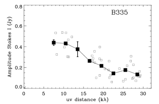
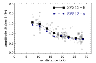
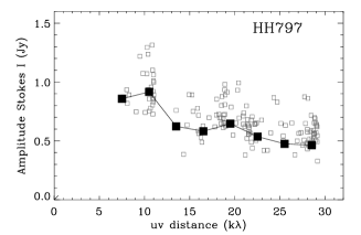
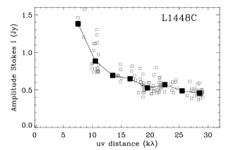
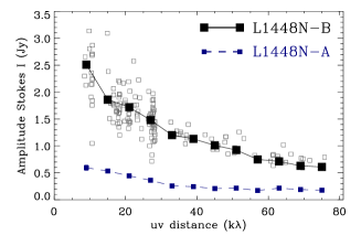
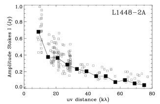
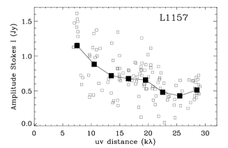
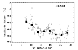
Figure 3: Stokes I visibility amplitude as a function of uv distance (in units of k$\lambda$). The open squares are the amplitudes of the visibilities channel-averaged and time-averaged every 120s. The black squares are derived averaging these amplitudes of the visibilities in 6 k$\lambda$ bins for L1448N, L1448-2A, NGC 1333 IRAS4A, IRAS4B and IRAS16293 and 3 k$\lambda$ bins for the other sources. For the wide-binary L1448N, SVS13 and IRAS16293, we model and isolate the two sources separately. For IRAS4B, we also isolate and remove NGC 1333 IRAS4B2 from the visibility data.

3 Results

3.1 0.87mm continuum fluxes

The 0.87mm dust continuum maps are presented in Fig. 2 (the Stokes I dust continuum emission is described in appendix A). We overlay the outflow direction (references from the literature can be found in Table 6). We provide the peak intensities and the integrated 0.87mm flux densities in Table 4. We also provide the associated masses calculated using the relation from Hildebrand (1983):

$$M=\frac{S_{\nu}\leavevmode\nobreak\ \mathcal{D}\leavevmode\nobreak\ d^{2}}{\kappa_{\nu}\leavevmode\nobreak\ B_{\nu}(T)}$$ (5)

with S_ν the flux density, $\cal{D}$ the dust-to-gas mass ratio assumed to be 0.01, d the distance to the protostar, $\kappa_{\nu}$ the dust opacity (tabulated in Ossenkopf & Henning (1994), 1.85 cm² g^-1 at 0.87mm) and B_ν(T) the Planck function. We choose a dust temperature of 25K, coherent with that observed at 1000 au in IRAS16293 by Crimier et al. (2010). A dust temperature of 50K would only decrease the gas mass reported in Table 4 by a factor of $\sim$2.

The sensitivity of SMA observations decreases outside the primary beam (i.e. 34″) and the coverage of the shortest baselines is not complete: we thus expect that only part of the total envelope flux will be recovered by our SMA observations, especially for the closest sources. To estimate how much of the extended flux is missing, we compare the SMA fluxes with those obtained with the SCUBA single-dish instrument. Di Francesco et al. (2008) provide a catalogue of 0.87mm continuum fluxes and peak intensities for a large range of objects observed with SCUBA at 450 and 850 $\mu$m, including our sources. The SCUBA integrated flux uncertainties are dominated by the 15% calibration uncertainties while the absolute flux uncertainty for the SMA is $<$10%. Results are summarized in Table 5. We find that the SMA total flux, integrated in the reconstructed cleaned maps of the sources, accounts for 9 – 18% of the SCUBA total fluxes. This is consistent with the results of the PROSAC low-mass protostar survey for which only 10 – 20% of the SCUBA flux is recovered with the SMA (Jørgensen et al., 2007). As far as the dust continuum peak flux densities are concerned, if we rescale the SCUBA peak flux densities to the one expected in the SMA beam, assuming that the intensity scales with radius (i.e. a density dependence $\rho\leavevmode\nobreak\ \propto\leavevmode\nobreak\$r^-2), we find that SCUBA and SMA peak flux densities are consistent with each other. This means that most of the envelope flux is recovered at SMA beam scales. The largest discrepancies appear for B335, NGC 1333 IRAS4A and NGC 1333 IRAS4B. For B335, the SCUBA value is twice that derived with SMA. This indicates that for this source, one of the closest of our sample, part of the SMA continuum flux might be missing even at the peak of continuum emission, and the polarization fraction could be lower than that determined from the SMA observations ($\S$3). For NGC 1333 IRAS4A and IRAS4B, the inverse is observed: the SMA peak value is 2 and 4 times larger than the rescaled SCUBA. The two sources are the most compact envelopes of the sample (Looney et al., 2003; Santangelo et al., 2015). The difference is thus probably due to beam dilution of the compact protostellar cores in the large SCUBA beam as well as possible contamination of the SCUBA fluxes due to the fact that NGC 1333 IRAS4A and B are both located within a long (1′$\times$40″) filamentary cloud extending southeast-northwest (Lefloch et al., 1998).

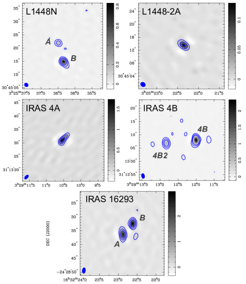
Figure 4: 345GHz dust continuum emission in L1448N, L1448-2A, NGC 1333 IRAS4A, NGC 1333 IRAS4B and IRAS16293 when only visibilities above 40 k$\lambda$ are kept. We apply a natural weighting to produce these maps. Contours at [5,20,50] $\sigma$ appear in blue. The beam sizes are $\sim$1$\aas@@fstack{\prime\prime}$9$\times$1$\aas@@fstack{\prime\prime}$2.

3.2 Analysis of the Stokes I visibilities

Part of the extended dust continuum emission is lost during the reconstruction of the final image itself, since an interferometer can only sparsely sample Fourier components of different spatial frequencies of the incoming signal. To analyze the impact of the map reconstruction on the flux values derived, we can compare the flux densities derived from the reconstructed map with those deduced directly from the visibility amplitude curves. The Stokes I amplitudes of the visibilities, averaged every 120s, are presented in Fig. 3. The sample includes three wide binary objects resolved by our SMA observations: L1448N, SVS13 and IRAS16293. We use the visibility data to separate the binary sources. As the sources cannot be modeled using a simple Gaussian fitting, we use the MIRIAD / imsub function to produce a sub-image containing L1448N-A, SVS13-A and IRAS16293-B from the cleaned image. We then use MIRIAD / uvmodel to subtract these sources from the visibility data and make an image of L1448N-B, SVS13-B and IRAS16293-A from the modified visibility datasets. We proceed the same way to independently map L1448N-A, SVS13-A and IRAS16293-B. The separated visibility profiles are shown in Fig. 3. The region mapped around NGC 1333 IRAS4B contained IRAS4A (outside the primary beam) and IRAS4B2 located about 10″ east of IRAS4B. These two sources are also isolated and removed from the visibility data presented in Fig. 3.

We use a Gaussian fitting method to fit the visibilities and extrapolate these models at 0 k$\lambda$ to derive the integrated 0.87mm continuum fluxes. The fluxes derived from the visibility amplitude curves are reported in Table 4. The fluxes derived from the visibility amplitude curves are close but, as expected, systematically larger (on average 2.2 times) than those derived on the reconstructed maps. We also indicate the 0.87mm continuum fluxes of L1448N-B and SVS13-B (the sources located at the phase center) in Table 4. We find that SVS13-A and B have similar fluxes while L1448N-B is 4 times brighter than L1448N-A.

For five sources, observations sampled baselines above 40k$\lambda$, i.e. sampling smaller spatial scales and most compact components of the envelope. We produce new maps of these sources using only visibilities that have a radius in the u-v plane larger than 40 k$\lambda$. We use a natural weighting scheme to produce the maps in order to achieve the highest point-source sensitivity. These maps are shown in Fig. 4. The flux densities of the compact components are $\sim$150, 25, 580, 530 and 1120mJy for L1448N, L1448-2A, NGC 1333 IRAS4A, NGC 1333 IRAS4B and IRAS16293 respectively: for L1448N and L1448-2A, the compact component only accounts for less than 1/10 of the total flux and for NGC 1333 IRAS4A and IRAS16293 for 1/4. This means that for these objects, most of the mass is still in the large-scale envelope rather than in a massive disk and that our SMA observations will allow to trace the polarized emission at the envelope scales where most of the mass resides, with only little contamination from a possible central protostellar disk. The visibility profile of NGC 1333 IRAS4B is the flattest in our sample (Fig. 3). 1/3 of the total 0.87mm flux is contained in the compact component. This flat visibility profile is consistent with those analyzed in Looney et al. (2003) and the ones obtained at both 1mm and 3mm by the IRAM-PdBI CALYPSO survey. The profile drops steeply at u$-$v distances larger than 60k$\lambda$, which suggests that NGC 1333 IRAS4B either has a compact (FWHM$<$6″) envelope or that its submm emission at scales 3 – 6″ is dominated by the emission from a large Gaussian disk-like structure. Note that both NGC 1333 IRAS4A and IRAS4B have very compact envelopes (envelope outer radii $<$ 6″) as seen with the PdBI observations at 1mm and 3mm (Maury et al. in prep).

3.3 Polarization results

Figure 9 shows the maps of the Stokes Q and U parameters and the polarization intensity and polarization fraction maps obtained when combining them. The peak polarization intensities and the median polarization fractions (defined as the unweighted ratio between the median polarization intensity over the flux intensity) are listed in Table 4. In spite of their low luminosity at SMA scales, we detect linearly polarized continuum emission in all the low-mass protostars, even using a conservative 3-$\sigma$ threshold. Median polarization fractions range from a few % for IRAS16293 and L1448N to 10% for B335. We only obtain a weak 2-$\sigma$ detection toward the northeastern companion of SMME/HH797 (around 03:43:57.8; +32:03:11.3). This object was classified as a Class 0 proto-brown dwarf candidate by Palau et al. (2014). When polarization is detected in the center, we observe that the polarization fraction drops toward this center. For HH797, L1448C, L1448-2A and IRAS03282, we detect polarization in the envelope at distances between 700 and 1600 au from the Stokes I emission peak, but not in the center itself. The absence of polarization could be linked with an averaging effect at high column density in the beam and/or along the line-of-sight in those objects. We analyze potential causes for depolarization in $\S$4.1.

4 Analysis and discussion

4.1 Distribution of the polarized emission

Polarization is detected in all of our maps, but not always towards the peak of dust continuum emission (Stokes I). A constant polarization fraction would predict on the contrary that the polarized intensity scales as Stokes I. Yet, polarization ‘holes’ or depolarization are often observed in the high-density parts of star-forming molecular cores and protostellar systems (Dotson, 1996; Rao et al., 1998; Wolf et al., 2003; Girart et al., 2006; Tang et al., 2013; Hull et al., 2014). We analyse the distribution of both polarized fraction and intensity in this section in order to probe if and where depolarization is observed.

4.1.1 Variation of the polarized fraction with environment

For sources where polarization is detected within the central 5″, we observe a drop in the polarization fraction (Fig. 9). To quantify this decrease, we analyze how the polarization fraction varies as a function of the 0.87mm flux density. We first re-generate our polarization maps with an homogeneous synthesized beam of 5.5″ in all our sources, using independent pixels 1/3 the synthesized beam (1.8″). IRAS 4A and B are not included in this analysis because their dust continuum emission is barely resolved at 5.5″. L1448-2A is not either since polarization is not robustly detected anymore at this new resolution. The relation linking p_frac versus the Stokes I flux density in each individual protostellar envelope is shown in Fig. 5 (top). The continuum flux densities is normalized to the peak intensity for each object to allow a direct comparison. We observe a clear depolarization toward inner envelopes with higher Stokes I fluxes, with a polarization fraction $\propto$ I^-0.6 for B335 down to $\propto$ I^-1.0 for L1448N or HH797. Those coefficient are consistent with results from the literature: the polarization fraction has, for instance, been found $\propto I^{-0.6}$ in Bok globules (Henning et al., 2001), $\propto I^{-0.7}$-I^-0.8 in dense cores (Matthews & Wilson, 2000) and down to $\propto I^{-0.97}$ in the main core of NGC 2024 FIR 5 (Lai et al., 2002).

Since polarization ‘holes’ are usually associated with a high-density medium, we also analyze how the polarization fraction varies as a function of the gas column density N(H₂). We assume that the emission at 0.87$\mu$m is optically thin. The column density is derived using the formula from Schuller et al. (2009):

$$N(\rm H_{2})=\frac{S_{\nu}}{\mathcal{D}\leavevmode\nobreak\ \mu_{\rm H_{2}}\leavevmode\nobreak\ m_{\rm H}\leavevmode\nobreak\ \Omega\leavevmode\nobreak\ \kappa_{\nu}\leavevmode\nobreak\ B_{\nu}(T)}$$ (6)

with S_ν the flux density, $\mu_{H_{2}}$ the molecular weight of the ISM ($\mu_{H_{2}}$=2.8; from Kauffmann et al. 2008), m_H the mass of an hydrogen atom, $\Omega$ the solid angle covered by the beam, $\kappa_{\nu}$ the dust opacity (tabulated in Ossenkopf & Henning (1994), 1.85 cm² g^-1 at 0.87mm) and B_ν(T) the Planck function at a dust temperature T. The dust-to-gas mass ratio $\cal{D}$ is assumed to be 0.01.

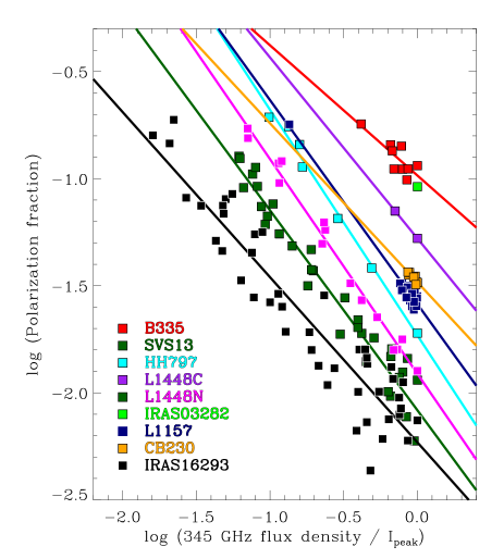
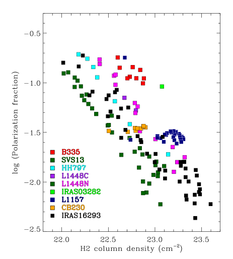
Figure 5: Polarization fractions as a function of Stokes I continuum intensities at 0.87mm (top) or as a function of the H₂ column densities (bottom). Maps have been regenerated to share a common synthesized beam of about 5.5″ and rebinned to have a grid with a common pixel size of 1.8″. The continuum flux densities plotted in the top panel are in units of Jy/beam but are normalized to the peak intensity for each object. The solid lines are the best fit to the function p${}_{frac}\propto$ (I/I_max)^a. The H₂ column densities plotted on the bottom panel are in units of cm^-2 and are derived using Eq. 5 and 6.

The temperature is not constant throughout the object envelopes: we assume that the temperature profile in optically thin outer envelopes follows T(r) $\propto$ r^-0.4 and scale the profiles using the protostellar internal luminosities (Terebey et al., 1993).

$$T=38\leavevmode\nobreak\ L_{int}^{0.2}\leavevmode\nobreak\ \left(\frac{\rm r}{100au}\right)^{-0.4}$$ (7)

Internal luminosities L_int were calculated from Herschel Gould Belt Survey in Sadavoy et al. (2014) for the Perseus sources and from Maury et al. (in prep) for the other sources. L_int was approximated to the bolometric luminosity if no internal luminosity could be found in the literature. Figure 5 (bottom) presents the dependency of p_frac with local column density. Even if the relation observed presents a large scatter, our results confirm that the polarization fraction decreases with increasing column density in the envelopes of our sample.

Along with the polarization fraction variations, the distribution of polarized emission intensities can also help us determine the cause of depolarization. SCUBAPOL observations have shown that the polarization intensity can decrease at high densities (Crutcher et al., 2004). We do not observe such trend in our sample. In Fig. 5, the slope of the polarization fraction relation with the dust continuum intensity is close to -1 or flatter for most sources. This means that the polarization intensity is constant and even increases (i.e. B335, SVS13 or IRAS16293) toward the central regions (see also the polarization intensity and fraction maps provided in Fig 9). These results suggest that for these sources, the decrease of the polarization fraction in the center is not linked with a full depolarization but could indicate a variation in the polarization efficiency itself (see next section).

SCUBA                             SMA

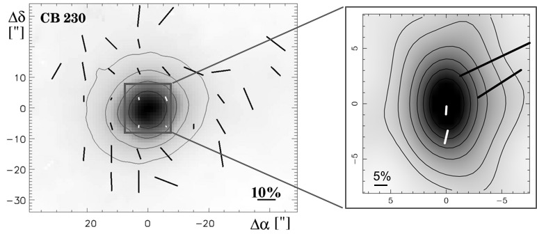
Figure 6: Left: SCUBA 0.85mm continuum maps with polarization orientation overlaid from Wolf et al. (2003). The contour lines mark 20%, 40%, 60%, and 80% of the maximum intensity. Right: Zoom-in into the scales covered with the SMA at 0.87mm. The contours are the same than in Fig. 2. For both, the bar length is proportional to the polarization fraction.

4.1.2 Potential causes for depolarization

Observations as well as models or simulations (Padoan et al., 2001; Bethell et al., 2007; Falceta-Gonçalves et al., 2008; Kataoka et al., 2012) have shown that depolarization can be linked with both geometrical effects (e.g. averaging effects linked with the complex structure of the magnetic field along the line of sight) as well as physical effects (e.g. collisional/mechanical disalignment, lower grain alignment efficiency, variation of the grain population). We discuss here some of these ‘depolarization’ effects. We note that our sample is sensitivity limited, which means that there is a potential bias toward strong polarization intensities. We also remind the reader that the polarized emission presented in this paper comes from the envelope and that we are not sampling the polarized (or unpolarized) emission from the inner ($<500$ au) envelope here.

Geometrical effects - Our SMA observations recover polarized emission from previously reported “polarization holes” observed with single-dish observations. Observations of B335 and CB230 at a 2200 au resolution using SCUBAPOL (Holland et al., 1999) performed by Wolf et al. (2003) show that the polarization fraction decreases from 6 – 15% in the outer parts of the cores to a few %, thus at scales where 3 – 10% polarization is detected with the SMA (see Fig. 6 for an illustration in CB230). The central depolarization observed by Wolf et al. (2003) in B335 and CB230 is thus partially due to beam averaging effects or mixing of the polarized signal along the line-of-sight, an envelope pattern that our SMA resolution now allows to recover. Recent polarization observations of B335 with ALMA at even higher resolution by Maury et al. (2018) confirm that polarization is still detected towards the center of the B335 envelope at 0.5 – 5″ scales, a sign that the dust emission stays polarized (p $\sim$ 3 – 7%) at small scales in the high density regions.

Optical depth effects - As already reported in Girart et al. (2006), a two-lobe distribution of the polarization intensity is detected toward NGC 1333 IRAS4A. We report a similar two-lobe structure for the first time in NGC 1333 IRAS4B, with peaks of the polarization intensity on each side of the north-south outflow. Liu et al. (2016) find that the polarization intensity of NGC 1333 IRAS4A observed at 6.9mm has a more typical distribution, with the polarization intensity peaking toward the source center and attributed this variation of the polarization distribution with wavelength to optical depth effects. Our temperature brightnesses rather suggest that the 0.87mm emission is optically thin at the envelope scales probed in this paper, for all our objects. We note that modeling the magnetic field in NGC 1333 IRAS4A, Gonçalves et al. (2008) show that strong central concentrations of magnetic field lines could reproduce a two-lobe structure in the polarized intensity distribution.

Grain alignment, grain growth - Several studies of dense molecular clouds or starless cores have shown that the slope of the polarization degree can reach values of ‘-1’ (as in some of our objects) or lower with respect to A_V or I/I_max and interpret this slope as a sign of a decrease or absence of grain alignment at higher densities (Alves et al., 2014; Jones et al., 2015, 2016). Even if we are not in such case (our objects all have a central heating source), the degree of polarization we detect is still extremely sensitive to the efficiency of grain alignment, which is itself very sensitive to the grain size distribution and potential grain growth (Bethell et al., 2007; Pelkonen et al., 2009; Brauer et al., 2016). This grain growth has been already suggested in Class 0 protostars like L1448-2A or L1157 (Kwon et al., 2009), with a faster grain growth toward the central regions. More observations combining different sub-mm wavelengths at various scales will help us probe the dust spectral index throughout the envelope, analyse the scales at which grain growth is expected (Chacón-Tanarro et al., 2017), probe the various environmental dependences of the grain alignment efficiency (Whittet et al., 2008) and observationally constrain the dependence on the polarization degree and the grain size as predicted for instance by radiative torque models (see Bethell et al., 2007; Hoang & Lazarian, 2009; Andersson et al., 2015; Jones et al., 2015).

4.2 Orientation of the magnetic field

The B-field lines are inferred from the polarization angles by applying a 90$\degr$ rotation. The mean magnetic field orientations in the central 1000 au are provided in Table 6. The B orientation is overlaid with red bars in Figure 2. We also show the $>$2-$\sigma$ detections (orange bars): although these are subject to higher uncertainties we stress that they are mostly consistent with the neighboring 3-$\sigma$ detection line segments. For robustness, however, these lower significance detections are not used in this analysis. Under flux-freezing conditions, the pull of field lines in strong gravitational potentials is expected to create an hourglass morphology of the magnetic field lines, centered around the dominant infall direction, during protostellar collapse. Using CARMA observations, Stephens et al. (2013) show that in L1157, the full hourglass morphology becomes apparent around 550 au. Using SMA observations, Girart et al. (2006) also observed this hourglass shape in NGC 1333 IRAS4A. The resolution we select for this analysis of B at envelope scale is not sufficient to reveal the hourglass morphology in most of our objects. Only one of our sources, L1448-2A, shows hints of an hourglass shape at envelope scales (see Fig. 2) but the non detection of polarization in the northern quadrant does not allow to detect a full hourglass pattern in this source: better sensitivity observations are needed to confirm this partial detection.

4.2.1 Large scales versus small scales

Our B-field orientations can be compared to SHARP 350$\mu$m and SCUBAPOL 850$\mu$m polarization observations that provide the orientation of the magnetic field at the surrounding cloud/filament scales for half of our sample. We use the SHARP results presented in Attard et al. (2009), Davidson et al. (2011) and Chapman et al. (2013) and the SCUBAPOL of Wolf et al. (2003) and Matthews et al. (2009). The large scale and smaller scale B orientations match for NGC 1333 IRAS4A, L1448N, L1157, CB230 and HH797. The SMA B orientation in L1448-2A is quite different from that detected with SHARP. In B335, the SCUBA observations seem also inconsistent (north-south direction) with the SMA B orientation. However, only two significant line segments are robustly detected with SCUBA and Bertrang et al. (2014) detect a mostly poloidal field in the B335 core using near-infrared polarization observations at 10000 au scales. Recent observations of B335 with ALMA have revealed a very ordered topology of the magnetic field structure at 50 au, with a combination of a large-scale poloidal magnetic field (outflow direction) and a strongly pinched magnetic field in the equatorial direction (Maury et al., 2018). Our SMA observations suggest that above $>$1000 au scales, the poloidal component dominates in B335. All these results show that an ordered B morphology from the cloud to the envelope is observed for most of our objects. Our results also seem to confirm that sources with consistent large-to-small-scale fields (e.g. B335, NGC 1333 IRAS4A, L1157 and CB230) tend to have a high polarization fraction , similar to what is found in Hull et al. (2013).

4.2.2 Variation of the B orientation with wavelength

Only few studies have investigated the relationship between the magnetic field orientation and wavelength on similar scales. Using single-dish observations, Poidevin et al. (2010) found that in star-forming molecular clouds, most of the 0.35 and 0.85mm polarization data had a similar polarization pattern. In Fig. 7, we compare the 0.87mm SMA B-field orientation to those observed at 1.3mm by Stephens et al. (2013) and Hull et al. (2014). CARMA maps are rebinned to match the grid of our SMA maps. 7 objects are common to the two samples and have co-spatial detections. We do not compare the SMA and CARMA results for B335 and L1448C, as polarization is only marginally ($<$3.5-$\sigma$) detected at 1.3 mm (Hull et al., 2014). The orientations at 0.87 and 1.3mm match for L1157, SVS13, L1448N-B, NGC 1333 IRAS4A and IRAS4B. For SVS13-B, the orientations only slightly deviate in the southeast part, but the position angles remain consistent within the uncertainties added in quadrature (8$\degr$ uncertainties for SMA, 14$\degr$ for CARMA). In L1448N-B, the orientation of the B-field, perpendicular to the outflow, is also consistent with BIMA (Berkeley Illinois Maryland Array; Welch et al., 1996) 1.3mm observations presented in Kwon et al. (2006). The orientations at 0.87 and 1.3mm deviate in the outer parts of the envelope in NGC 1333 IRAS4B, in regions with low detected polarized intensities. In CB230, the 3-$\sigma$ detection at 0.87 and 1.3mm do not exactly overlap physically but the east-west orientation of our central detections is consistent with the orientation found with CARMA by Hull et al. (2014). For L1448-2A finally, the SMA 0.87 and CARMA 1.3mm detections do not overlap, making a direct comparison between wavelength difficult for this object. We note that the flat structure of the dust continuum emission oriented northeast-southwest observed at 0.87mm is consistent with that observed at 1.3 mm by Yen et al. (2015). The 1.3mm observations from TADPOL are not in agreement: a northwest-southeast extension is observed along the outflow, the polarization detections (blue bars in Fig. 7) from TADPOL in the central part of L1448-2A might be suffering from a contaminating by CO polarized emission from the outflow itself. Their 2.5-$\sigma$ detections along the equatorial plane are, however, consistent with our 2-$\sigma$ detections. Our conclusion is that the orientations observed at 0.87 and 1.3mm are consistent. Those two wavelengths being close to each other, they probably trace optical depths on which the magnetic field orientations stay ordered.

Figure 7: B-field orientation derived from SMA 0.87mm observations in red (3-$\sigma$ detections) and from CARMA 1.3mm observations in blue (3.5-$\sigma$ detections from Hull et al., 2014). The underlying map is the polarization intensity in mJy/beam and contours are the Stokes I continuum emission (same levels as in Fig. 2).

4.2.3 Misalignment with the outflow orientation

Whether or not the rotation axis of protostellar cores are aligned with the main magnetic field direction is still an open question. From an observational point of view, it remains difficult to precisely pinpoint the rotation axis of protostellar cores. The outflow axis is often used as a proxy for this key parameter, as protostellar bipolar outflows are believed to be driven by hydromagnetic winds in the circumstellar disk (Pudritz & Norman, 1983; Shu et al., 2000; Bally, 2016). The core rotation and outflow axes are thus usually considered as aligned. Synthetic observations of magnetic fields in protostellar cores have shown that magnetized cores have strong alignments of the outflow axis with the B orientation while less magnetized cores present more random alignment (Lee et al., 2017). MHD collapse models predict in particular that magnetic braking should be less effective if the envelope rotation axis and the magnetic field are not aligned (Hennebelle & Ciardi, 2009; Joos et al., 2012; Krumholz et al., 2013; Li et al., 2013). The comparison between the rotation axis and the B-field orientation is thus a key to understand the role of B in regulating the collapse. Previous observational works found that outflows do not seem to show a preferential direction with respect to the magnetic field direction both on large scales (Curran & Chrysostomou, 2007) and at 1000 au scales (Hull et al., 2013). A similar absence of correlation is also reported in a sample of high-mass star-forming regions by Zhang et al. (2014). Our detections of the main B-field component at envelope scales for all the protostars of our sample allow us to push the analysis further for low-mass Class 0 objects.

The misalignments between the B orientation and the outflow axis driven by the protostars can be observed directly from Figure 2. Table 6 provides the projected position angle of the outflows as well as the angle difference between this outflow axis and the main envelope magnetic field orientation when B is detected in the central region. For half of the objects, the magnetic field lines are oriented within 40$\degr$ of the outflow axis but some sources show rather large ($>$60$\degr$) difference of angles (e.g. L1448N-B and CB230). Using the maps generated with a common 5.5″ synthesized beam (thus excluding NGC 1333 IRAS 4A, 4B and L1448-2A, see $\S$4.1), we build a histogram of the projected angles between the magnetic field orientation and the outflow direction (hereafter $\cal{A}$_B-O) shown in Fig. 8. We also compare the full histogram with that restricted to detections within the central 1500 au (Fig. 8, bottom panel). The distribution of $\cal{A}$_B-O looks roughly bimodal, suggesting that at the scales traced with the SMA, the B-field lines are either aligned or perpendicular to the outflow direction. Hull et al. (2014) find hints that for objects with low polarization fractions, the B-field orientations tend to be preferentially perpendicular to the outflow. In our sample focusing on solar-type Class 0 protostars, we do not observe a relation between $\cal{A}$_B-O and the polarization fraction nor intensity. For instance, L1448N-B and SVS13-B have very similar polarization fractions but very different $\cal{A}$_B-O. In the same way, the two Bok globules B335 and CB230 both have a high polarization fraction but exhibit very different $\cal{A}$_B-O.

Table 6: Misalignment between the outflow angles $\chi$_o and the mean magnetic field orientation $\chi$_B1000 in the central 1000 au.

Name	$\chi$oa	$\chi$B1000	$\lvert$ $\chi$o - $\chi$B1000 $\rvert$
	($\degr$)	($\degr$)
B335	90	55$\pm$3	35
SVS13-A	148	140$\pm$3	8
SVS13-B	160	19$\pm$6	39
HH797	150	113$\pm$2	37
L1448C	161	-	-
L1448N-B	105	23$\pm$5	82
L1448-2A	138	-	-
IRAS03282	120	-	-
NGC 1333 IRAS4A	170	57$\pm$13	67
NGC 1333 IRAS4B	0	58$\pm$49	58
IRAS16293-A	145	163$\pm$15	18
IRAS16293-B	130	114$\pm$17	16
L1157	146	146$\pm$4	0
CB230	172	86$\pm$3	86

• Position angles are provided east of north. References: Bachiller et al. (1998), Bachiller et al. (2001), Choi (2001), Hull et al. (2013), Hull et al. (2014), Rodríguez et al. (1997), Tafalla et al. (2006), Rao et al. (2009), Santangelo et al. (2015), Yen et al. (2015).

Figure 8: Histogram of the projected angles between the magnetic field and the outflow direction. The data share a common synthesized beam size of about 5.5″ and are binned with pixels of 1.8″ for this analysis. The top panel shows the histogram color-coded per source while the bottom panel shows the global histogram (in white) with the histogram restricted to detections within the central 1500 au overlaid in gray.

4.2.4 A relation between misaligned magnetic field, strong rotation and fragmentation?

Details on the various velocity gradients (orientation, strength) measured in our sources are provided in appendix. Velocity fields in protostars can trace many processes (turbulence, outflow motions, etc.). In particular, gradients detected in the equatorial plane of the envelope can trace both rotation and infall motions. Organized velocity gradients with radius are often interpreted as a sign that the rotational motions dominate the velocity field. In this section, we compare the B orientation and the misalignment $\cal{A}$_B-O with velocity gradients associated with rotation in our envelopes.

$\cal{A}$_B-O $>$ 45$\degr$ case - L1448N-B and CB230 have a $\cal{A}$_B-O close to 90$\degr$. They both have large envelope masses and velocity gradients perpendicular to their outflow direction detected at hundreds of au scales. A high rotational to magnetic energy could lead to a twist of the field lines in the main rotation plane. Their high mass-to-flux ratio $\mu=M/\Phi\sim E_{grav}/E_{mag}$ could also favor a gravitational pull of the equatorial field lines. Both scenarios can efficiently produce a toroidal/radial field from an initially poloidal field that would explain the main field component we observe perpendicular to the outflow/rotation axis. The opposite causal relationship is also possible: an initially misaligned magnetic field configuration could be less efficient at braking the rotation and lead to the large rotational motions detected at envelope scales. Additional observations of Class 0 from the literature show similar misalignments. In NGC 1333 IRAS2A, the B direction is misaligned with the outflow axis (Hull et al., 2014) but aligned with the velocity gradient observed in the combined PdBI+IRAM30 C¹⁸O map by Gaudel et al. (in prep). In L1527, $\cal{A}$_B-O is nearly 90$\degr$ (Segura-Cox et al., 2015) but the B direction follows the clear north-south velocity gradient tracing the Keplerian rotation of a rather large $\sim$60 au disk (Ohashi et al., 2014). We stress out, however, that polarization in disks could also be produced by the self-scattering of dust grains (Kataoka et al., 2015) and not tracing B. Finally, our source NGC 1333 IRAS4A has a B orientation misaligned compared to the small scale north-south outflow direction (see also Girart et al., 2006) but aligned with the large scale 45$\deg$ outflow direction (bended outflow; see appendix). This is consistent with the position angle of the velocity gradient found by Belloche et al. (2006), even if the interpretation of gradients is difficult in IRAS4A because strong infall motions probably dominate the velocity field.

$\cal{A}$_B-O $<$ 45$\degr$ case - We find only small misalignments in L1157 and B335, sources that show low to no velocity gradient at 1000 au scales (Tobin et al., 2011; Yen et al., 2010, Gaudel et al. in prep). The B orientation of the off-center detection in L1448C (see Fig. 2) is also aligned with the outflow axis. The source has one of the smallest velocity gradient perpendicular to the outflow axis determined by Yen et al. (2015). Our wide-multiple systems IRAS16293 (A and B) and SVS13 (A and B) present good alignments. IRAS16293-B does not show rotation but the source is face-on, which might explain the absence of rotation signatures. In IRAS16293-A, the magnetic field has an “hourglass” shape at smaller scales (Rao et al., 2009), a signature of strong magnetic fields in the source, but the source also has a strong velocity gradient perpendicular to the outflow direction that could be responsible for some of the misalignment. Finally, the B direction is slightly tilted in the center of SVS13B. We note that Chen et al. (2007) detected an extended velocity gradient detected along the SVS13-A/SVS13-B axis across the whole SVS13 system that has been interpreted as core rotation.

Even if our sample is limited, the coincidence of a misalignment of B with the outflow direction when large perpendicular velocity gradients are present or the alignment of B with the velocity gradient itself strongly suggests that the orientation of B at the envelope scales traced by the SMA can be affected by the strong rotational energy in the envelope. These results are consistent with predictions from numerical simulations that show a strong relation between the angular velocity of the envelope and the magnetic field direction (Machida et al., 2005, 2007). Rotationally twisted magnetic fields have already been observed at larger scales (Girart et al., 2013; Qiu et al., 2013). After a given number of periods, rotation could be distorting or even twisting the field lines, producing a toroidal component in the equatorial plane. Using MHD simulations, Ciardi & Hennebelle (2010) and Joos et al. (2012) showed that the mass ejection via outflows could be less efficient when the rotation axis and B direction are misaligned. The presence of outflows in sources with $\cal{A}$_B-O $\sim$ 90$\degr$ might favour a twisted/pinched magnetic field scenario compared to an initially misaligned magnetic field configuration.

Reinforcing the possible correlation between the field misalignment and the presence of strong rotational motions, our SMA observations also suggest that a possible correlation could be present between the envelope-scale main magnetic field direction and the multiplicity observed in the inner envelopes. Indeed, sources that present a strong misalignment (IRAS03282, NGC 1333 IRAS4A, L1448N, L1448-2A or CB230) are all close multiples (Launhardt, 2004; Chandler et al., 2005; Choi, 2005; Tobin et al., 2013, 2016, Maury et al. in prep). SVS13-A does host a close multiple but it is a Class I: we are thus not witnessing the initial conditions leading to fragmentation, and the magnetic field we observe could have been severely affected by the evolution of both the environment and the protostar itself. On the contrary, sources that show an alignment between the B direction and the outflow direction (e.g. L1157, B335, SVS13-B and L1448C) have been studied with ALMA or NOEMA high-resolution observations and stand as robust single protostars at envelope scales of $\sim$5000-10000 au. No large disk has been detected so far in these sources (Saito et al., 1999; Yen et al., 2010; Chiang et al., 2012; Tobin et al., 2015) while L1448N-B for instance was suggested recently to harbor a quite large disk encompassing several multiple sources at scales $\sim 100$ au (Tobin et al., 2016). These results support those of Zhang et al. (2014): the possible link between fragmentation and magnetic field topology points towards a less efficient magnetic braking and redistribution of angular momentum when the B-field is misaligned.

5 Summary

We perform a survey of 0.87mm continuum and polarized emission from dust toward 12 low-mass Class 0 protostars.

(i) By comparing the 0.87mm SMA continuum fluxes with single-dish observations, we find that our interferometric observations recover $<$20% of the total fluxes. The fluxes derived directly from the visibility data are also about twice larger than those derived on the reconstructed maps. For 5 objects, we observed baselines above 40 k$\lambda$ that allow us to separate the most compact components. The low flux fractions contained in the compact component are consistent with the classification as Class 0 of our sources.

(ii) We report the detection of linearly polarized dust emission in all the objects of the sample, with mean polarization fractions ranging from 2 to 10%.

(iii) We find a decrease of the polarization fraction with the estimated H₂ column density. Our polarization intensity profiles are relatively flat in most of our sources and increases toward the center in B335, SVS13 or IRAS16293, suggesting a decrease in the dust alignment efficiency rather than a polarization cancellation in these sources. Two-lobes structures in the polarized intensity distributions are observed in NGC 1333 IRAS4A and IRAS4B.

(iv) The orientations observed at 0.87mm with SMA and 1.3mm with CARMA are consistent with each other on the 1000 au scales probed in this analysis.

(v) Like in Hull et al. (2013), we find that sources with a high polarization fraction have consistent large-to-small-scale fields. We do not observe, however, a relation between the misalignment of the magnetic field orientation with respect to the outflow axis and the polarization intensity or fraction.

(vi) We find clues that large misalignment of the magnetic field orientation with the outflow orientation could be found preferentially in protostars with a higher rotational energy. The misalignment of 90$\degr$ observed in some objects could thus be a signature of winding of the magnetic field lines in the equatorial plane when the rotational energy is significant. Strengthening this possible link, there are also hints that a B-outflow misalignment is found preferentially in protostars that are close multiple and/or harbor a larger disk, while single objects seem to show a good agreement between the magnetic field direction at envelope scales and the direction of their protostellar outflow. This suggests that the topology and strength of magnetic fields at envelope scale may significantly impact the outcome of protostellar collapse, eventually playing a major role in the formation of disks and multiple systems.

Our results are aligned with previous studies of B in massive cores (Zhang et al., 2014) as well as with theoretical predictions from magnetic collapse models (Machida et al., 2005; Joos et al., 2012). More observations of the magnetic field of low-mass protostars at envelope scale would be necessary to observationally confirm these ‘tentative’ but promising results and re-enforce our interpretations.

Appendix A Source description

In this section, we provide a quick description of the objects and of the 0.87mm continuum observed with the SMA.

B335

B335 is an isolated Bok globule hosting a Class 0 protostar. Its luminosity is $\sim$1$L_{\sun}$ (Keene et al. 1983) and its mass $<$2$M_{\sun}$.

Ouflows - It possesses an east-west elongated, conical-shaped molecular outflow (PA: 80$\degr$; Hirano et al. 1988). Collimated ¹²CO (2$-$1) jets (Yen et al. 2010) and Herbig-Haro (HH) objects (HH 119 A$-$F; Reipurth et al. 1992; Gâlfalk & Olofsson 2007) are detected along this outflow axis.

Velocity field - C¹⁸O (2$-$1) and H¹³CO⁺ (1$-$0) interferometric observations have traced the rotational infalling motion of the envelope from radii of $\sim 20000$ down to $\sim 1000$ au. No clear rotational motion is detected on 100-500 au scales (Saito et al. 1999; Harvey et al. 2003; Yen et al. 2011) and the central circumstellar disk radius is estimated to be smaller than 100 au.

Our SMA observations - The SMA 0.87mm continuum emission has a north-south elongated structure coherent with previous 1.3mm observations of the object by Motte & André (2001). The two protuberances observed in the north and southwest regions trace the edge of the cavity produced by the horizontal outflow (Yen et al. 2010).

SVS13

SVS13 is a multiple system in the NGC 1333 star-forming region. It possesses 3 main submm continuum sources aligned in the northeast-southwest direction named A, B and C (Looney et al. 2003). SVS13-A is a Class I protostar while SVS13-B and C are Class 0. A large filamentary structure encompasses the three sources at 450 $\mu$m (Chandler & Richer 2000) and in mm (Hull et al. 2014). The combined luminosity for SVS13-A, B, and C is 45$L_{\sun}$ (Jennings et al. 1987). 70 $\mu$m emission is detected toward SVS13-A and C but not toward SVS13-B, suggesting that the source is deeply embedded (Chen et al. 2009). A radio source called VLA3 has also been detected southwest of SVS13-A (Rodríguez et al. 1997).

Ouflows - SVS13-A is likely powering the strong northwest-southeast HH7-11 outflow studied by Bachiller et al. (2000) and Plunkett et al. (2013). SVS13-B is known to drive a highly collimated SiO jet (Bachiller et al. 1998).

Velocity field - A symmetric velocity gradient of 28km s${}^{-1}\leavevmode\nobreak\$pc^-1 across SVS13-B and SVS13A/VLA3 has been detected using N₂H⁺ observations. This large gradient could suggest that the wide binary system is physically bound (Chen et al. 2009).

Our SMA observations - The SMA 0.87mm observations trace the extended envelope around SVS13-A and SVS13-B. We resolve the two sources while SVS13-C is only marginally detected in the southwest. The continuum emission of SVS13-A is slightly elongated in the southwest direction, toward the position of VLA3. The 0.87mm emission of SVS13-B extends in the north-northwest direction. That extension aligns with that of the SiO jet driven by the protostar. The continuum emission also extends in the southwest direction of SVS13-B: the extension is also observed in the elongated N₂H⁺ map but not in the PdBI 1.4 and 3 mm observations, which could be linked with filtering effects affecting the PdBI maps (Chen et al. 2009).

IC348-SMM2 / HH797

SMM2 is a low-mass class 0 belonging to the IC 348 star-forming region. SMA observations also reveal a companion source, SMM2E, at $\sim$2400 au in the northeast direction (Palau et al. 2014) whose Spectral Energy Distribution is typical of Class 0 objects.

Ouflows - SMM2 probably drives the HH797 jet, a very extended and collimated northwest-southeast outflow (Chen et al. 2013). Velocity asymmetries along the length of the flow were interpreted as jet rotation (Pech et al. 2012). A compact low-velocity outflow seems to also be associated with SMM2E.

Velocity field - C¹⁸O observations of the companion source SMM2E suggest that the envelope is probably rotating with a north-south axis close to the outflow direction (Palau et al. 2014).

Our SMA observations - Our 0.87mm continuum map is consistent with that previously obtained by Palau et al. (2014) with SMA as well as far-IR continuum emission observed with Herschel. Both SMM2 and SMM2E are detected at 0.87mm, but SMME2 is not resolved.

L1448C

The L1448C complex (also called L1448-mm) hosts several embedded Class 0 protostars (Tobin et al. 2007).

Ouflows - It possesses well collimated outflows (Hirano et al. 2010). The northern CO lobe is probably interacting with the neighboring source L1448N (Bachiller et al. 1995).

Velocity field - VLA observations of NH₃ reveal velocity gradients perpendicular to the outflow as well as along the outflow axis. This suggests the presence of a self-gravitating structure around L1448C, with an envelope that is both rotating and contracting at comparable velocities (Curiel et al. 1999).

Our SMA observations - Our SMA observations show that L1448C is elongated in the northwest-southeast direction, which is consistent with the elongation observed at 1.3mm (Barsony et al. 1998). The southeast elongation encompasses the companion source L1448-mm B (2000 au separation) observed with Spitzer (Tobin et al. 2007) (also called L1448C(S); Jørgensen et al. 2006). A distortion is also observed in the southwest direction where a 0.80mm continuum emission has been observed by Barsony et al. (1998). This distortion as well as the northern elongation could also be tracing the edge of the outflow cavities.

L1448N

L1448N (or L1448 IRS3) is a multiple system. L1448N-A is located 2100 au north to L1448N-B. B is the strongest source at mm wavelengths (Looney et al. 2000) while A dominates at mid-IR (Ciardi et al. 2003) and cm wavelengths (Curiel et al. 1990). The system is also connected to L1448NW located 20″ north. Barsony et al. (1998) suggest that star formation in L1448N could have been induced by the strong outflow driven by L1448C (see also Kwon et al. 2006).

Ouflows - Two bipolar outflows originate from the system. The outflow driven by L1448N-A is nearly perpendicular to the line-of-sight. Kwon et al. (2006) show that the two outflows are probably interacting with each other.

Velocity field - The inner 5-10″ of L1448N presents a solid-body rotation while the outer envelope shows a flatter profile (Terebey & Padgett 1997). C¹⁸O observations also reveal a strong velocity gradient ($>$100 km s ^-1 pc^-1; Gaudel et al. in prep; Yen et al. 2015) perpendicular to the outflow direction within 20$\degr$ (Lee et al. 2015).

Our SMA observations - L1448N-A and B are resolved by the SMA while L1448NW is marginally detected. Both sources are elongated in the northeast-southwest direction, which is consistent with previous 230 GHz and 0.87mm SMA observations by Lee et al. (2015).

L1448-2A

L1448-2A (or L1448 IRS 2) is a low luminosity (5.2 $L_{\odot}$) Class 0 protostar located toward the western edge of the L1448 complex that seems to be evolving in isolation from L1448N and C.

Ouflows - High-velocity CO maps show that L1448-2A drives an outflow in the northwest-southeast direction (O’Linger et al. 1999). Additional studies from Wolf-Chase et al. (2000) suggest that the source is actually driving two distinct outflows, which could be a signature of an (unresolved) binary system.

Velocity field - Using C¹⁸O observations, Yen et al. (2015) found a velocity gradient nearly perpendicular to the outflow axis.

Our SMA observations - The northeast-southwest extension of the envelope is confirmed by our SMA observation. Contrary to the CARMA 1.3 mm dust continuum presented in Hull et al. (2014), we do not observe elongation in the northwest-southeast direction. As this elongation is not observed at other wavelengths, we conclude that the elongation observed at 1.3 mm might be due to contamination by the outflow. The ‘horns’ detected in the east and west direction trace the edges of the large outflow cavity.

IRAS03282

IRAS03282 is a highly-embedded Class 0 object lying at 1$\degr$ southeast of NGC 1333 (Jørgensen et al. 2006). IRAS 03282 possesses two sources separated by 1.5″ (Launhardt 2004).

Outflows - The source drives an outflow in which various velocity components are observed, in particular a high-velocity ($\sim$60km s^-1) jet with fast molecular clumps detected along the outflow axis surrounded by a less collimated and more standard velocity ($\sim$20km s^-1) outflow (Bachiller et al. 1991).

Velocity field - N₂H⁺ and NH₃ observations were used to trace the large-scale velocity gradient of the envelope that is mostly distributed along the outflow direction (Tobin et al. 2011).

Our SMA observations - The N₂H⁺ and NH₃ maps present an elongation along the north-south direction. Our SMA 0.87mm map presents a similar elongation. The southern elongation is also very similar to that observed at 350$\mu$m by Wu et al. (2007) with SHARC-II.

NGC 1333 IRAS4A

NGC 1333 IRAS4A is a Class 0 object located in the south of NGC 1333. It hosts two sources (IRAS4A1 and IRAS4A2) in a close (1.8″) binary pair that was resolved with interferometers at submm and mm wavelengths using the SMA or BIMA (Looney et al. 2000; Girart et al. 2006; Jørgensen et al. 2007) and more recently ALMA (López-Sepulcre et al. 2017): IRAS4A1 dominates the submm and mm emission.

Outflows - An arcmin-long outflow, seen in high-velocity CO(3-2) emission, is associated with IRAS4A2 and bends from a north-south orientation on small scales (Santangelo et al. 2015) to a position angle of 45$\circ$ on large scales Koumpia et al. (2016). This could be due to an intrinsic change of the gas propagation direction, or a signature of jet precession. The launching direction of the outflow driven by IRAS4A1 is also oriented close to north-south direction and faster (Santangelo et al. 2015). Part of that SiO outflow (position angle of -10$\degr$) was also reported by Choi (2001).

Velocity field - Detections of inverse P-Cygni profiles in the lines of common molecular species such as ${}^{13}CO$ or CS are interpreted as signs of strong infall motions of the outer cloud (Di Francesco et al. 2001; Jørgensen et al. 2007). Belloche et al. (2006) detected a centroid velocity gradient of about 10 km s ^-1 pc^-1, with a position angle of 38$\degr$, while Ching et al. (2016) find a velocity gradient along the axis linking NGC 1333 IRAS4A1 and IRAS4A2. Both Belloche et al. (2006) and Gaudel et al (in prep.) show however that the interpretation of these velocity gradients in terms of rotation is not straightforward in IRAS4A due to the strong infall motions previously mentioned.

Our SMA observations - As already shown in Girart et al. (2006), the SMA 0.87mm map presents a very compact structure extended in the A1-A2 direction. The common envelope extends in the northeast and southwest direction, in the same direction ($\sim$30-50$\degr$) i) that the velocity gradient found in Belloche et al. (2006), ii) that the outflow takes further from the protostar and iii) that the large-scale B orientation observed by SCUBA (Matthews et al. 2009).

NGC 1333 IRAS4B

NGC 1333 IRAS4B is also a Class 0 protostar and belongs to the same N₂H⁺ arcmin-scale filament as IRAS4A. Submm and mm observations reveal a second source located 11″ on the east (IRAS4B2) (Looney et al. 2000). IRAS4B2 is not detected at cm wavelengths, suggesting that it is at a different stage of its evolution (Reipurth et al. 2002) or just not associated at all with IRAS4B. There are still some debate on smaller scales on whether the disk of IRAS 4B is observed face- or edge-on (Watson et al. 2007; Marvel et al. 2008).

Outflows - The source is driving an outflow whose axis is nearly in north-south direction. Its short dynamical timescale suggests that this outflow is very young (Choi 2001).

Velocity field - IRAS4B seems to be collapsing (Di Francesco et al. 2001; Belloche et al. 2006) but does not show clear signs of rotational motions at 1000 au scales (Yen et al. 2013).

Our SMA observations - The SMA 0.87mm map of IRAS4B presents a very compact structure that seems to be extended in the north-south direction, namely the direction of the outflow emanating from this source. We do not observe the same east-west extension as seen at 1.3 mm by Hull et al. (2014) and Yen et al. (2013).

IRAS16293

IRAS16293 is a Class 0 protostar system located in the $\rho$ Ophiuchi molecular cloud. It possesses a bolometric luminosity of $\sim$25$L_{\sun}$ and a massive envelope (Correia et al. 2004; Crimier et al. 2010) surrounding two cores separated by 6″, called A (south) and B (north). Crimier et al. (2010) suggests that IRAS16293A/B is a “separate envelope system” (following the classification proposed by Looney et al. 2003). IRAS16293-A is an edge-on system and IRAS16293-B is nearly face-on (Jørgensen et al. 2016). The first dominates the system luminosity. SMA observations have also enabled to separate IRAS16293-A into two components, Aa and Ab, aligned along a position angle of 45$\degr$ (Chandler et al. 2005). No small scale multiplicity has been found for IRAS16293-B.

Outflows - The source shows significant outflow activity. While IRAS16293-A seems to be driving the main east-west CO outflow, the driving source of the northwest-southeast compact outflow (PA of 145$\degr$) traced with SiO observations is still unclear (Yeh et al. 2008; Rao et al. 2009). This much younger outflow is probably a more robust tracer of the rotation axis, as recent studies revealed at various scales an almost edge-on rotational pattern whose axis match the SiO outflow orientation Pineda et al. (2012); Girart et al. (2014). A one-sided bubble-like outflow structure originates from IRAS16293-B in the southeast direction (Loinard et al. 2013).

Velocity field - In IRAS16293-A, C³⁴S observations reveal a clear velocity gradient along PA 40-45$\degr$, i.e. perpendicular to the SiO-traced outflow (Girart et al. 2014) probably due to infalling motion of the rotating envelope. A disk-like rotation is also detected at 40 – 60 au with ALMA, with the same orientation (Oya et al. 2016). In IRAS16293-B, recent ALMA observations reveal inverse P-Cygni profiles toward the center of IRAS16293-B in the CH₃OCHO-A CH₃OCHO-E and H₂CCO lines, here again indicative of infall motions (Pineda et al. 2012). The source is observed face-on: no rotation has been detected.

Our SMA observations - As shown in Rao et al. (2009), the SMA 0.87mm observations separate the two A and B components. IRAS16293-B is brighter than IRAS16293-A. The continuum emission of the envelope extends in the north of IRAS16293-A and is also quite extended ($\sim$10″) toward its southeast direction, i.e. in the direction of the redshifted part of the SiO outflow.

L1157

L1157 is a low-mass Class 0 protostar and seems to be a single system (Tobin et al. 2013).

Outflows - It possesses a spectacular bipolar outflow asymmetric on large-scales. Its prominent CO cavities are likely created by the propagation of large bow-shocks (also traced via the NH₃ or SiO molecular lines; Tafalla & Bachiller 1995; Zhang et al. 1995; Gueth et al. 1996). This could be the sign that a time-variable collimated jet is driving the outflow (Podio et al. 2016).

Velocity field - L1157 has a flattened and filamentary envelope presenting a weak velocity gradient along the filament - thus perpendicular to the outflow. Broad linewidths are observed in the inner envelope (see Kwon et al. 2015).

Our SMA observations - Our 0.87mm observations are consistent with those presented in (Chen et al. 2013). Neither Chen et al. (2013) nor our observations detect the elongation structure detected at 1.3 mm with Stephens et al. (2013) in the northern (outflow) direction. By contrast, we detect a similar eastern extension and western bump. This horizontal elongation is also observed at 350$\mu$m by Wu et al. (2007).

CB230

CB 230 is an isolated globule hosting a dense core, itself hosting two deeply embedded YSOs. These are separated by 10″ and are aligned in the east-west direction (Launhardt 2001, 2004). The eastern object, IRS2 is not detected beyond 24 $\mu$m (Massi et al. 2008; Launhardt et al. 2013).

Outflows - The north-south CO outflows seem to be driven by the western protostar IRS1. More recent 7mm high-resolution observations of IRS1 led to the detection of two continuum sources separated by $\sim$100au, with an unresolved primary source at the origin of the outflow and an extended companion source located in a direction perpendicular to the outflow direction (Tobin et al. 2013).

Velocity field - CB230 presents a velocity gradient $>$10 km s ^-1 pc^-1 increasing from east to west along the axis connecting the two embedded YSOs (Chen et al. 2007; Tobin et al. 2011). The gradient is perpendicular to the outflow axis.

Our SMA observations - The 0.87mm continuum emission of CB230 is elongated in a boxy-shaped like structure in the north-south direction, an elongation also observed at 1.3mm by Hull et al. (2014). The southwest elongation could here again be linked with emission tracing the edges of the north-south outflow cavity.

Appendix B Stokes Q and U, polarization intensity and fraction maps of the sample

Figure 9: Continued. Same for IRAS03282, L1157 and CB230.

Figure 9: Continued. Same for NGC 1333 IRAS4A, NGC 1333 IRAS4B and IRAS16293.

References

- Alves et al. (2014) Alves, F. O., Frau, P., Girart, J. M., et al. 2014, A&A, 569, L1
- Andersson et al. (2015) Andersson, B.-G., Lazarian, A., & Vaillancourt, J. E. 2015, ARA&A, 53, 501
- Andre et al. (1993) Andre, P., Ward-Thompson, D., & Barsony, M. 1993, ApJ, 406, 122
- Andre et al. (2000) Andre, P., Ward-Thompson, D., & Barsony, M. 2000, Protostars and Planets IV, 59
- Attard et al. (2009) Attard, M., Houde, M., Novak, G., et al. 2009, ApJ, 702, 1584
- Bachiller et al. (2000) Bachiller, R., Gueth, F., Guilloteau, S., Tafalla, M., & Dutrey, A. 2000, A&A, 362, L33
- Bachiller et al. (1995) Bachiller, R., Guilloteau, S., Dutrey, A., Planesas, P., & Martin-Pintado, J. 1995, A&A, 299, 857
- Bachiller et al. (1998) Bachiller, R., Guilloteau, S., Gueth, F., et al. 1998, A&A, 339, L49
- Bachiller et al. (1991) Bachiller, R., Martin-Pintado, J., & Planesas, P. 1991, A&A, 251, 639
- Bachiller et al. (2001) Bachiller, R., Pérez Gutiérrez, M., Kumar, M. S. N., & Tafalla, M. 2001, A&A, 372, 899
- Bally (2016) Bally, J. 2016, ARA&A, 54, 491
- Barsony et al. (1998) Barsony, M., Ward-Thompson, D., André, P., & O’Linger, J. 1998, ApJ, 509, 733
- Belloche (2013) Belloche, A. 2013, in EAS Publications Series, Vol. 62, EAS Publications Series, ed. P. Hennebelle & C. Charbonnel, 25–66
- Belloche et al. (2006) Belloche, A., Hennebelle, P., & André, P. 2006, A&A, 453, 145
- Bertrang et al. (2014) Bertrang, G., Wolf, S., & Das, H. S. 2014, A&A, 565, A94
- Bethell et al. (2007) Bethell, T. J., Chepurnov, A., Lazarian, A., & Kim, J. 2007, ApJ, 663, 1055
- Bock et al. (2006) Bock, D. C.-J., Bolatto, A. D., Hawkins, D. W., et al. 2006, in Proc. SPIE, Vol. 6267, Society of Photo-Optical Instrumentation Engineers (SPIE) Conference Series, 626713
- Bodenheimer (1995) Bodenheimer, P. 1995, ARA&A, 33, 199
- Bontemps et al. (1996) Bontemps, S., Andre, P., Terebey, S., & Cabrit, S. 1996, A&A, 311, 858
- Brauer et al. (2016) Brauer, R., Wolf, S., & Reissl, S. 2016, A&A, 588, A129
- Caselli et al. (2002) Caselli, P., Benson, P. J., Myers, P. C., & Tafalla, M. 2002, ApJ, 572, 238
- Chacón-Tanarro et al. (2017) Chacón-Tanarro, A., Caselli, P., Bizzocchi, L., et al. 2017, A&A, 606, A142
- Chandler et al. (2005) Chandler, C. J., Brogan, C. L., Shirley, Y. L., & Loinard, L. 2005, ApJ, 632, 371
- Chandler & Richer (2000) Chandler, C. J. & Richer, J. S. 2000, ApJ, 530, 851
- Chapman et al. (2013) Chapman, N. L., Davidson, J. A., Goldsmith, P. F., et al. 2013, ApJ, 770, 151
- Chen et al. (2013) Chen, X., Arce, H. G., Zhang, Q., et al. 2013, ApJ, 768, 110
- Chen et al. (2007) Chen, X., Launhardt, R., & Henning, T. 2007, ApJ, 669, 1058
- Chen et al. (2009) Chen, X., Launhardt, R., & Henning, T. 2009, ApJ, 691, 1729
- Chiang et al. (2012) Chiang, H.-F., Looney, L. W., & Tobin, J. J. 2012, ApJ, 756, 168
- Ching et al. (2016) Ching, T.-C., Lai, S.-P., Zhang, Q., et al. 2016, ApJ, 819, 159
- Choi (2001) Choi, M. 2001, ApJ, 553, 219
- Choi (2005) Choi, M. 2005, ApJ, 630, 976
- Ciardi & Hennebelle (2010) Ciardi, A. & Hennebelle, P. 2010, MNRAS, 409, L39
- Ciardi et al. (2003) Ciardi, D. R., Telesco, C. M., Williams, J. P., et al. 2003, ApJ, 585, 392
- Correia et al. (2004) Correia, J. C., Griffin, M., & Saraceno, P. 2004, A&A, 418, 607
- Crimier et al. (2010) Crimier, N., Ceccarelli, C., Maret, S., et al. 2010, A&A, 519, A65
- Crutcher (2012) Crutcher, R. M. 2012, ARA&A, 50, 29
- Crutcher et al. (2004) Crutcher, R. M., Nutter, D. J., Ward-Thompson, D., & Kirk, J. M. 2004, ApJ, 600, 279
- Curiel et al. (1990) Curiel, S., Raymond, J. C., Moran, J. M., Rodriguez, L. F., & Canto, J. 1990, ApJ, 365, L85
- Curiel et al. (1999) Curiel, S., Torrelles, J. M., Rodríguez, L. F., Gómez, J. F., & Anglada, G. 1999, ApJ, 527, 310
- Curran & Chrysostomou (2007) Curran, R. L. & Chrysostomou, A. 2007, MNRAS, 382, 699
- Davidson et al. (2011) Davidson, J. A., Novak, G., Matthews, T. G., et al. 2011, ApJ, 732, 97
- Di Francesco et al. (2008) Di Francesco, J., Johnstone, D., Kirk, H., MacKenzie, T., & Ledwosinska, E. 2008, ApJS, 175, 277
- Di Francesco et al. (2001) Di Francesco, J., Myers, P. C., Wilner, D. J., Ohashi, N., & Mardones, D. 2001, ApJ, 562, 770
- Dotson (1996) Dotson, J. L. 1996, ApJ, 470, 566
- Enoch et al. (2011) Enoch, M. L., Corder, S., Duchêne, G., et al. 2011, ApJS, 195, 21
- Evans et al. (2015) Evans, II, N. J., Di Francesco, J., Lee, J.-E., et al. 2015, ApJ, 814, 22
- Evans et al. (2009) Evans, II, N. J., Dunham, M. M., Jørgensen, J. K., et al. 2009, ApJS, 181, 321
- Falceta-Gonçalves et al. (2008) Falceta-Gonçalves, D., Lazarian, A., & Kowal, G. 2008, ApJ, 679, 537
- Frau et al. (2011) Frau, P., Galli, D., & Girart, J. M. 2011, A&A, 535, A44
- Gâlfalk & Olofsson (2007) Gâlfalk, M. & Olofsson, G. 2007, A&A, 475, 281
- Galli et al. (2006) Galli, D., Lizano, S., Shu, F. H., & Allen, A. 2006, ApJ, 647, 374
- Girart et al. (1999) Girart, J. M., Crutcher, R. M., & Rao, R. 1999, ApJ, 525, L109
- Girart et al. (2014) Girart, J. M., Estalella, R., Palau, A., Torrelles, J. M., & Rao, R. 2014, ApJ, 780, L11
- Girart et al. (2013) Girart, J. M., Frau, P., Zhang, Q., et al. 2013, ApJ, 772, 69
- Girart et al. (2006) Girart, J. M., Rao, R., & Marrone, D. P. 2006, Science, 313, 812
- Gonçalves et al. (2008) Gonçalves, J., Galli, D., & Girart, J. M. 2008, A&A, 490, L39
- Goodman et al. (1993) Goodman, A. A., Benson, P. J., Fuller, G. A., & Myers, P. C. 1993, ApJ, 406, 528
- Gueth et al. (1996) Gueth, F., Guilloteau, S., & Bachiller, R. 1996, A&A, 307, 891
- Harvey et al. (2003) Harvey, D. W. A., Wilner, D. J., Myers, P. C., & Tafalla, M. 2003, ApJ, 596, 383
- Hennebelle & Ciardi (2009) Hennebelle, P. & Ciardi, A. 2009, A&A, 506, L29
- Henning et al. (2001) Henning, T., Wolf, S., Launhardt, R., & Waters, R. 2001, ApJ, 561, 871
- Hildebrand (1983) Hildebrand, R. H. 1983, QJRAS, 24, 267
- Hirano et al. (2010) Hirano, N., Ho, P. P. T., Liu, S.-Y., et al. 2010, ApJ, 717, 58
- Hirano et al. (1988) Hirano, N., Kameya, O., Nakayama, M., & Takakubo, K. 1988, ApJ, 327, L69
- Hirota et al. (2008) Hirota, T., Bushimata, T., Choi, Y. K., et al. 2008, PASJ, 60, 37
- Hirota et al. (2011) Hirota, T., Honma, M., Imai, H., et al. 2011, PASJ, 63, 1
- Ho et al. (2004) Ho, P. T. P., Moran, J. M., & Lo, K. Y. 2004, ApJ, 616, L1
- Hoang & Lazarian (2009) Hoang, T. & Lazarian, A. 2009, ApJ, 695, 1457
- Holland et al. (1999) Holland, W. S., Robson, E. I., Gear, W. K., et al. 1999, MNRAS, 303, 659
- Hull et al. (2017) Hull, C. L. H., Girart, J. M., Tychoniec, Ł., et al. 2017, ApJ, 847, 92
- Hull et al. (2013) Hull, C. L. H., Plambeck, R. L., Bolatto, A. D., et al. 2013, ApJ, 768, 159
- Hull et al. (2014) Hull, C. L. H., Plambeck, R. L., Kwon, W., et al. 2014, ApJS, 213, 13
- Jennings et al. (1987) Jennings, R. E., Cameron, D. H. M., Cudlip, W., & Hirst, C. J. 1987, MNRAS, 226, 461
- Jones et al. (2015) Jones, T. J., Bagley, M., Krejny, M., Andersson, B.-G., & Bastien, P. 2015, AJ, 149, 31
- Jones et al. (2016) Jones, T. J., Gordon, M., Shenoy, D., et al. 2016, AJ, 151, 156
- Joos et al. (2012) Joos, M., Hennebelle, P., & Ciardi, A. 2012, A&A, 543, A128
- Jørgensen et al. (2007) Jørgensen, J. K., Bourke, T. L., Myers, P. C., et al. 2007, ApJ, 659, 479
- Jørgensen et al. (2006) Jørgensen, J. K., Harvey, P. M., Evans, II, N. J., et al. 2006, ApJ, 645, 1246
- Jørgensen et al. (2016) Jørgensen, J. K., van der Wiel, M. H. D., Coutens, A., et al. 2016, A&A, 595, A117
- Kataoka et al. (2012) Kataoka, A., Machida, M. N., & Tomisaka, K. 2012, ApJ, 761, 40
- Kataoka et al. (2015) Kataoka, A., Muto, T., Momose, M., et al. 2015, ApJ, 809, 78
- Kauffmann et al. (2008) Kauffmann, J., Bertoldi, F., Bourke, T. L., Evans, II, N. J., & Lee, C. W. 2008, A&A, 487, 993
- Keene et al. (1983) Keene, J., Davidson, J. A., Harper, D. A., et al. 1983, ApJ, 274, L43
- Knude & Hog (1998) Knude, J. & Hog, E. 1998, A&A, 338, 897
- Koumpia et al. (2016) Koumpia, E., van der Tak, F. F. S., Kwon, W., et al. 2016, A&A, 595, A51
- Krumholz et al. (2013) Krumholz, M. R., Crutcher, R. M., & Hull, C. L. H. 2013, ApJ, 767, L11
- Kwon et al. (2015) Kwon, W., Fernández-López, M., Stephens, I. W., & Looney, L. W. 2015, ApJ, 814, 43
- Kwon et al. (2006) Kwon, W., Looney, L. W., Crutcher, R. M., & Kirk, J. M. 2006, ApJ, 653, 1358
- Kwon et al. (2009) Kwon, W., Looney, L. W., Mundy, L. G., Chiang, H.-F., & Kemball, A. J. 2009, ApJ, 696, 841
- Lai et al. (2002) Lai, S.-P., Crutcher, R. M., Girart, J. M., & Rao, R. 2002, ApJ, 566, 925
- Launhardt (2001) Launhardt, R. 2001, in IAU Symposium, Vol. 200, The Formation of Binary Stars, ed. H. Zinnecker & R. Mathieu, 117
- Launhardt (2004) Launhardt, R. 2004, in IAU Symposium, Vol. 221, Star Formation at High Angular Resolution, ed. M. G. Burton, R. Jayawardhana, & T. L. Bourke, 213
- Launhardt et al. (2013) Launhardt, R., Stutz, A. M., Schmiedeke, A., et al. 2013, A&A, 551, A98
- Lazarian (2007) Lazarian, A. 2007, J. Quant. Spec. Radiat. Transf., 106, 225
- Lee et al. (2017) Lee, J. W. Y., Hull, C. L. H., & Offner, S. S. R. 2017, ApJ, 834, 201
- Lee et al. (2015) Lee, K. I., Dunham, M. M., Myers, P. C., et al. 2015, ApJ, 814, 114
- Lefloch et al. (1998) Lefloch, B., Castets, A., Cernicharo, J., Langer, W. D., & Zylka, R. 1998, A&A, 334, 269
- Li et al. (2014) Li, H.-B., Goodman, A., Sridharan, T. K., et al. 2014, Protostars and Planets VI, 101
- Li et al. (2013) Li, Z.-Y., Krasnopolsky, R., & Shang, H. 2013, ApJ, 774, 82
- Liu et al. (2016) Liu, H. B., Lai, S.-P., Hasegawa, Y., et al. 2016, ApJ, 821, 41
- Loinard et al. (2013) Loinard, L., Zapata, L. A., Rodríguez, L. F., et al. 2013, MNRAS, 430, L10
- Looney et al. (2000) Looney, L. W., Mundy, L. G., & Welch, W. J. 2000, ApJ, 529, 477
- Looney et al. (2003) Looney, L. W., Mundy, L. G., & Welch, W. J. 2003, ApJ, 592, 255
- Looney et al. (2007) Looney, L. W., Tobin, J. J., & Kwon, W. 2007, ApJ, 670, L131
- López-Sepulcre et al. (2017) López-Sepulcre, A., Sakai, N., Neri, R., et al. 2017, A&A, 606, A121
- Machida et al. (2007) Machida, M. N., Inutsuka, S.-i., & Matsumoto, T. 2007, ApJ, 670, 1198
- Machida et al. (2005) Machida, M. N., Matsumoto, T., Tomisaka, K., & Hanawa, T. 2005, MNRAS, 362, 369
- Marrone (2006) Marrone, D. P. 2006, PhD thesis, Harvard University
- Marrone & Rao (2008) Marrone, D. P. & Rao, R. 2008, in Proc. SPIE, Vol. 7020, Millimeter and Submillimeter Detectors and Instrumentation for Astronomy IV, 70202B
- Marvel et al. (2008) Marvel, K. B., Wilking, B. A., Claussen, M. J., & Wootten, A. 2008, ApJ, 685, 285
- Massi et al. (2008) Massi, F., Codella, C., Brand, J., di Fabrizio, L., & Wouterloot, J. G. A. 2008, A&A, 490, 1079
- Matthews et al. (2009) Matthews, B. C., McPhee, C. A., Fissel, L. M., & Curran, R. L. 2009, ApJS, 182, 143
- Matthews & Wilson (2000) Matthews, B. C. & Wilson, C. D. 2000, ApJ, 531, 868
- Maury et al. (2010) Maury, A. J., André, P., Hennebelle, P., et al. 2010, A&A, 512, A40+
- Maury et al. (2011) Maury, A. J., André, P., Men’shchikov, A., Könyves, V., & Bontemps, S. 2011, A&A, 535, A77
- Maury et al. (2014) Maury, A. J., Belloche, A., André, P., et al. 2014, A&A, 563, L2
- Maury et al. (2018) Maury, A. J., Girart, J. M., Zhang, Q., et al. 2018, accepted for publication in MNRAS
- Motte & André (2001) Motte, F. & André, P. 2001, A&A, 365, 440
- Ohashi et al. (2014) Ohashi, N., Saigo, K., Aso, Y., et al. 2014, ApJ, 796, 131
- O’Linger et al. (1999) O’Linger, J., Wolf-Chase, G., Barsony, M., & Ward-Thompson, D. 1999, ApJ, 515, 696
- Ossenkopf & Henning (1994) Ossenkopf, V. & Henning, T. 1994, A&A, 291, 943
- Oya et al. (2016) Oya, Y., Sakai, N., López-Sepulcre, A., et al. 2016, ApJ, 824, 88
- Padoan et al. (2001) Padoan, P., Goodman, A., Draine, B. T., et al. 2001, ApJ, 559, 1005
- Palau et al. (2014) Palau, A., Zapata, L. A., Rodríguez, L. F., et al. 2014, MNRAS, 444, 833
- Pech et al. (2012) Pech, G., Zapata, L. A., Loinard, L., & Rodríguez, L. F. 2012, ApJ, 751, 78
- Pelkonen et al. (2009) Pelkonen, V.-M., Juvela, M., & Padoan, P. 2009, A&A, 502, 833
- Pineda et al. (2012) Pineda, J. E., Maury, A. J., Fuller, G. A., et al. 2012, A&A, 544, L7
- Planck Collaboration (2016) Planck Collaboration. 2016, A&A, 586, A138
- Plunkett et al. (2013) Plunkett, A. L., Arce, H. G., Corder, S. A., et al. 2013, ApJ, 774, 22
- Podio et al. (2016) Podio, L., Codella, C., Gueth, F., et al. 2016, A&A, 593, L4
- Poidevin et al. (2010) Poidevin, F., Bastien, P., & Matthews, B. C. 2010, ApJ, 716, 893
- Pudritz & Norman (1983) Pudritz, R. E. & Norman, C. A. 1983, ApJ, 274, 677
- Qiu et al. (2013) Qiu, K., Zhang, Q., Menten, K. M., Liu, H. B., & Tang, Y.-W. 2013, ApJ, 779, 182
- Rao et al. (1998) Rao, R., Crutcher, R. M., Plambeck, R. L., & Wright, M. C. H. 1998, ApJ, 502, L75
- Rao et al. (2009) Rao, R., Girart, J. M., Marrone, D. P., Lai, S.-P., & Schnee, S. 2009, ApJ, 707, 921
- Reipurth et al. (1992) Reipurth, B., Heathcote, S., & Vrba, F. 1992, A&A, 256, 225
- Reipurth et al. (2002) Reipurth, B., Rodríguez, L. F., Anglada, G., & Bally, J. 2002, AJ, 124, 1045
- Rodríguez et al. (1997) Rodríguez, L. F., Anglada, G., & Curiel, S. 1997, ApJ, 480, L125
- Sadavoy et al. (2014) Sadavoy, S. I., Di Francesco, J., Andre, P., et al. 2014, ApJ, 787, L18
- Saito et al. (1999) Saito, M., Sunada, K., Kawabe, R., Kitamura, Y., & Hirano, N. 1999, ApJ, 518, 334
- Santangelo et al. (2015) Santangelo, G., Codella, C., Cabrit, S., et al. 2015, A&A, 584, A126
- Schuller et al. (2009) Schuller, F., Menten, K. M., Contreras, Y., et al. 2009, A&A, 504, 415
- Segura-Cox et al. (2016) Segura-Cox, D. M., Harris, R. J., Tobin, J. J., et al. 2016, ApJ, 817, L14
- Segura-Cox et al. (2015) Segura-Cox, D. M., Looney, L. W., Stephens, I. W., et al. 2015, ApJ, 798, L2
- Shu et al. (2000) Shu, F. H., Najita, J. R., Shang, H., & Li, Z.-Y. 2000, Protostars and Planets IV, 789
- Stephens et al. (2013) Stephens, I. W., Looney, L. W., Kwon, W., et al. 2013, ApJ, 769, L15
- Straizys et al. (1992) Straizys, V., Cernis, K., Kazlauskas, A., & Meistas, E. 1992, Baltic Astronomy, 1, 149
- Stutz et al. (2008) Stutz, A. M., Rubin, M., Werner, M. W., et al. 2008, ApJ, 687, 389
- Tafalla & Bachiller (1995) Tafalla, M. & Bachiller, R. 1995, ApJ, 443, L37
- Tafalla et al. (2006) Tafalla, M., Kumar, M. S. N., & Bachiller, R. 2006, A&A, 456, 179
- Tang et al. (2013) Tang, Y.-W., Ho, P. T. P., Koch, P. M., Guilloteau, S., & Dutrey, A. 2013, ApJ, 763, 135
- Terebey et al. (1993) Terebey, S., Chandler, C. J., & Andre, P. 1993, ApJ, 414, 759
- Terebey & Padgett (1997) Terebey, S. & Padgett, D. L. 1997, in IAU Symposium, Vol. 182, Herbig-Haro Flows and the Birth of Stars, ed. B. Reipurth & C. Bertout, 507–514
- Tobin et al. (2013) Tobin, J. J., Chandler, C. J., Wilner, D. J., et al. 2013, ApJ, 779, 93
- Tobin et al. (2011) Tobin, J. J., Hartmann, L., Chiang, H.-F., et al. 2011, ApJ, 740, 45
- Tobin et al. (2016) Tobin, J. J., Looney, L. W., Li, Z.-Y., et al. 2016, ApJ, 818, 73
- Tobin et al. (2007) Tobin, J. J., Looney, L. W., Mundy, L. G., Kwon, W., & Hamidouche, M. 2007, ApJ, 659, 1404
- Tobin et al. (2015) Tobin, J. J., Looney, L. W., Wilner, D. J., et al. 2015, ApJ, 805, 125
- Watson et al. (2007) Watson, D. M., Bohac, C. J., Hull, C., et al. 2007, Nature, 448, 1026
- Welch et al. (1996) Welch, W. J., Thornton, D. D., Plambeck, R. L., et al. 1996, PASP, 108, 93
- Whittet et al. (2008) Whittet, D. C. B., Hough, J. H., Lazarian, A., & Hoang, T. 2008, ApJ, 674, 304
- Wolf et al. (2003) Wolf, S., Launhardt, R., & Henning, T. 2003, The Astrophysical Journal, 592, 233
- Wolf-Chase et al. (2000) Wolf-Chase, G. A., Barsony, M., & O’Linger, J. 2000, AJ, 120, 1467
- Wu et al. (2007) Wu, J., Dunham, M. M., Evans, II, N. J., Bourke, T. L., & Young, C. H. 2007, AJ, 133, 1560
- Yeh et al. (2008) Yeh, S. C. C., Hirano, N., Bourke, T. L., et al. 2008, ApJ, 675, 454
- Yen et al. (2015) Yen, H.-W., Koch, P. M., Takakuwa, S., et al. 2015, ApJ, 799, 193
- Yen et al. (2010) Yen, H.-W., Takakuwa, S., & Ohashi, N. 2010, ApJ, 710, 1786
- Yen et al. (2011) Yen, H.-W., Takakuwa, S., & Ohashi, N. 2011, ApJ, 742, 57
- Yen et al. (2013) Yen, H.-W., Takakuwa, S., Ohashi, N., & Ho, P. T. P. 2013, ApJ, 772, 22
- Zhang et al. (1995) Zhang, Q., Ho, P. T. P., Wright, M. C. H., & Wilner, D. J. 1995, ApJ, 451, L71
- Zhang et al. (2014) Zhang, Q., Qiu, K., Girart, J. M., et al. 2014, ApJ, 792, 116