CytonRL: an Efficient Reinforcement Learning
Open-source Toolkit Implemented in C++

Abstract

This paper presents an open-source enforcement learning toolkit named CytonRL . The toolkit implements four recent advanced deep Q-learning algorithms from scratch using C++ and NVIDIA’s GPU-accelerated libraries. The code is simple and elegant, owing to an open-source general-purpose neural network library named CytonLib. Benchmark shows that the toolkit achieves competitive performances on the popular Atari game of Breakout.

1 Introduction

Reinforcement learning (RL) is self learning what to do under an environment, in other words, how to map situations to actions, so as to maximize a numerical reward signal Sutton and Barto (1998). RL is an meaningful artificial intelligence task, and will be extremely useful if it works. However, traditional real-world RL systems were usually built upon hand-crafted features from raw sensor data, which is a bottleneck of their performance. Therefore, learning to control agents directly from high-dimensional sensory inputs was considered as one of the long-standing challenges of RL.

Recently, the deep learning community has developed deep neural networks to automatically extract high-level features from raw sensory data, leading to breakthroughs in computer vision LeCun et al. (1998); Krizhevsky et al. (2012); Farabet et al. (2013); Sermanet et al. (2013); Mnih (2013) and speech recognition Povey et al. (2014); Dahl et al. (2012); Graves et al. (2013). Excitingly, the RL community integreted this technology into their systems, and achieved the long-standing challenge Mnih et al. (2013, 2015).

The breakthrough in RL will undoubtedly give birth to impressive progress in the related fields such as natural language processing and robotics. Therefore, we develop the open-source toolkit of CytonRL in the hope to benefit research communities as well as industries.

CytonRL is an open-source toolkit of deep Q-learning. It achieves competitive performances on the test environment of Atari 2600 test-bed Bellemare et al. (2013) through following the works as,

Deep Q-Network(DQN) proposed by Mnih et al. (2013) and Mnih et al. (2015);

Double DQN proposed by van Hasselt et al. (2015);

Prioritized Experience Replay proposed by Schaul et al. (2015);

Dueling DQN proposed by Wang et al. (2015).

In addition, the parameter settings of CytonRL has been carefully tuned for both efficiency and effectiveness.

CytonRL is built from scratch using C++ and NVIDIA’s GPU-accelerated libraries, sharing the same strategy as the neural machine translation toolkit of CytonMT Wang et al. (2018). The advantages of CytonRL includes,

Running Efficiency

through better exploiting the power of GPU compared to the toolkit implemented in other languages, since C++ language is the genuine official language of NVIDIA – the manufacturer of the GPU hardware;

Code Simplicity

owing to an C++ open-source general-purpose neural network library named CytonLib which is shipped as part of the source code.

Programming Flexibility

as all low-level operations are visible to users.

The following of this paper is organized as: the section 2 descirbes the methods used in the toolkit of CytonRL; the section 3 explains the implmentation; the section 4 presents the benchmark; the section 5 concludes this paper.

2 Method

CytonRL has implemented four recent advanced deep Q-learning algorithms proposed by Mnih et al. (2013); van Hasselt et al. (2015); Schaul et al. (2015); Wang et al. (2015). The following subsections first introduce the background knowledge of reinforcement learning, and then present the details of these four algorithms.

2.1 Background

Suppose an agent interacts with an environment $\mathcal{E}$ in a sequence of actions, observations, and rewards (Mnih et al., 2013). At each time-step,the agent selects an action $a_{t}$ from the set of legal game actions, $A=\{1,\ldots,K\}$. The action is passed to $\mathcal{E}$ and modifies its internal state. The agent both receives an reward $r_{t}$ and makes an new observation $x_{t+1}$ from $\mathcal{E}$.

Most often the observation $x_{t}$ does not fully specify the internal state of $\mathcal{E}$. Therefore, the sequence of actions and observations $s_{t}=x_{1},a_{1},x_{2},a_{2},\ldots,a_{t-1},x_{t}$ are considered as an representation of $\mathcal{E}$’s state, upon which strategies are learned.

The goal of the agent is to interact with $\mathcal{E}$ by selecting actions in a way that maximizes future rewards. There is an standard assumption that future rewards are discounted by a factor of $\gamma$ per time-step, as $\mathcal{E}$ is generally stochastic. The future discounted return at the time $t$ is defined as

$$R_{t}=\sum_{t^{\prime}=t}^{T}\gamma^{t^{\prime}-t}r_{t^{\prime}},$$ (1)

where $T$ is the time-step at which $\mathcal{E}$ decides to terminate.

In order to deduce the optimal policy, a helper function named optimal action-value function is defined as the maximum expected return achievable by following any strategy, after seeing some sequence $s$ and then taking some action $a$, formulated as,

$$Q^{*}(s,a)=\mathop{max}_{\pi}\mathbb{E}[R_{t}|s_{t}=s,a_{t}=a,\pi],$$ (2)

where $\pi$ is a policy mapping a sequence to actions or distributions over actions.

The optimal policy can be derived after knowing $Q^{*}(s,a)$, formulated as,

$$a^{*}(s)=\mathop{argmax}_{a}Q^{*}(s,a).$$ (3)

The optimal action-value function obeys the Bellman equation,

$$Q^{*}(s,a)=\mathbb{E}[r+\gamma\mathop{max}_{a^{\prime}}Q^{*}(s^{\prime},a^{\prime})|s,a],$$ (4)

where $s^{\prime}$ is any sequence derived by taking $a$ after seeing $s$.

2.2 Deep Q-Network with Experience Replay

Deep Q-Network (DQN) uses a neural network to approximate the optimal action-value function $Q^{*}(s,a)$. The network is trained by minimizing a sequence of loss functions at each iteration $i$, as

$$L_{i}(\theta_{i})=\mathop{\mathbb{E}}_{s,a\thicksim\rho(\cdot)}\left[\left(y_{i}-Q(s,a;\theta_{i})\right)^{2}\right]$$ (5)

where $y_{i}=\mathbb{E}_{s^{\prime}\thicksim\mathcal{E}}[r+\gamma\mathop{max}_{a^{\prime}}Q(s^{\prime},a^{\prime};\theta_{i-1})|s,a]$ is a boosted target for the iteration $i$, and $\rho(s,a)$ is a probability distribution over $s$ and $a$ referred as behavior distribution. Differentiating the loss functions with respect to the weights leads to,

$$\nabla_{\theta_{i}}L_{i}(\theta_{i})=\mathop{\mathbb{E}}_{\begin{array}[]{c}s,a\thicksim\rho(.)\\ s^{\prime}\thicksim\mathcal{E}\end{array}}\left[-\left(r+\gamma\mathop{max}_{a^{\prime}}(s^{\prime},a^{\prime};\theta_{i-1})-Q(s,a;\theta_{i})\right)\nabla_{\theta_{i}}Q(s,a;\theta_{i})\right].$$ (6)

DQN simplifies the computation through replacing the expection by single samples from the $\rho$ and $\mathcal{E}$, forumlated as,

$$\nabla_{\theta_{i}}L_{t}(\theta_{i})=-\left(r_{t}+\gamma\mathop{max}_{a^{\prime}}Q(s_{t+1},a^{\prime};\theta_{i-1})-Q(s_{t},a_{t};\theta_{i})\right)\nabla_{\theta_{i}}Q(s_{t},a_{t};\theta_{i}).$$ (7)

Mnih et al. (2013) proposed utilizing an experience replay technique in DQN, presented by the algorithm 1. The approach stores the agent’s experiences at each time-step formulated as $e_{t}=(s_{t},a_{t},r_{t},s_{t+1})$, into a replay memory as $\mathcal{D}=e_{1},\ldots,e_{N}$. The approach then picks random samples from $\mathcal{D}$ for updating the neural network.

DQN with experience replay is dramatically more efficient and stable than the standard online Q-learning Sutton and Barto (1998). The reasons are as follows Mnih et al. (2013).

• Learning directly from consecutive samples is inefficient due to the strong correlations between the samples; randomizing the samples breaks these correlations and therefore reduces the variance of updates.

• When learning on-policy, the current parameters determine the next data sample that the parameters are trained on; By using experience replay the behavior distribution is averaged over many of its previous states, smoothing out learning and voiding oscillations or divergence in the parameters.

• Each step of experience is potentially used in many weight updates, which allows for greater data efficiency.

Algorithm 1 Deep Q-Network with Experience Replay

1:Initialize the replay memory $\mathcal{D}$ to capacity $N$

2:Initialize the action-value function $\mathcal{Q}$ with random weights

3:for episode = $1$, $M$ do

4:     Initialize sequence $s_{1}=\{x_{1}\}$ and preprocessed $\phi_{1}=\phi(s_{1})$

5:     for $t$ = $1$, $T$ do

6:         With probability $\epsilon$ select a random action $a_{t}$

7:         otherwise select $a_{t}=\mathop{argmax}_{a}Q^{*}(\phi(s_{t}),a;\theta)$

8:         Execute action $a_{t}$ in emulator and observe reward $r_{t}$ and image $x_{t+1}$

9:         Set $s_{t+1}=s_{t},a_{t},x_{t+1}$ and preprocess $\phi_{t+1}=\phi(s_{t+1})$

10:         Store transition $(\phi_{t},a_{t},r_{t},\phi_{t+1})$ in $\mathcal{D}$

11:         Sample random minibatch of transitions $(\phi_{j},a_{j},r_{j},\phi_{j+1})$ from $\mathcal{D}$

12:         Set $y_{j}=\left\{\begin{array}[]{ll}r_{j}&\textrm{for terminal}\phi_{j+1}\\ r_{j}+\gamma\mathop{max}_{a^{\prime}}Q(\phi_{j+1},a^{\prime};\theta)&\textrm{for non-terminal}\phi_{j+1}\\ \end{array}\right.$

13:         Perform a gradient descent step on $(y_{j}-Q(\phi_{j}a_{j};\theta))^{2}$ using the equation 7

14:     end for

15:end for

2.3 Double Deep Q-Network

van Hasselt et al. (2015) proposed double DQN to reduce the over-estimations caused by the max operation in the equation 7.

The standard DQN used a training target as,

$$Y_{t}^{DQN}=r_{t}+\gamma\mathop{max}_{a}Q(s_{t+1},a;\theta_{t}^{-}),$$ (8)

where $\theta_{t}^{-}$ is the parameters of a target network which is copied periodically from the online network. Because DQN is a kind of boosting algorithm, the estimated target $Q(s_{t+1},a;\theta_{t}^{-})$ is unavoidably inaccurate as an oracle function during the training procedure. This inaccuracy is high likely to be converted into over-estimations by the max operation.

Double DQN decomposes the max operation in the equation 8 into action selection and action evaluation, formulated as,

$$Y_{t}^{DoubleDQN}=r_{t}+\gamma Q(s_{t+1},argmaxQ(s_{t+1},a;\theta_{t}),\theta_{t}^{-}),$$ (9)

where the online network with the parameters $\theta_{t}$ is used to evaluate the greedy policy, and the target network with the parameters $\theta_{t}^{-}$ is used to estimate its values.

2.4 Prioritized Experience Replay

Schaul et al. (2015) proposed prioritized experience replay to improve the learning efficiency of DQN, presented by the algorithm 2. The intuition of the method is to replay important transitions more frequently.

The probability of sampling a transition $i$ is defined as,

$$P(i)=\frac{p_{i}^{\alpha}}{\sum_{k}p_{k}^{\alpha}}$$ (10)

where $p_{i}>0$ is the priority of the transition $i$. The exponent $\alpha$ determines how much prioritization is used, with $\alpha=0$ corresponding to the uniform case.

The priority $p_{i}$ in the proportional prioritization method, which is implemented in CytonRL, is defined as,

$$p_{i}=|\delta_{i}|+\epsilon,$$ (11)

where $\delta_{i}$ is the prediction error, and $\epsilon$ is a small positive constant that prevents the edge-case of transitions not being revisited once their error is zero.

Prioritized experience replay changes the sampling distribution, which brings bias to the estimation. Importance-sampling is used to compensate this bias, formulated as

$$w_{i}=(\frac{1}{N}\cdot\frac{1}{P(i)})^{\beta}$$ (12)

where $0\leqslant\beta\leqslant 1$ controls the strength of compensation.

Algorithm 2 Double DQN with Proportional Prioritized Experience Replay

1:minibatch $k$, step-size $\eta$, replay period $K$ and size $N$, exponents $\alpha$ and $\beta$, budget $T$.

2:Initialize replay memory $\mathcal{H}$ to capacity $N$, $\Delta=0$, $p_{1}=1$.

3:Observe $s_{1}$

4:for t = $1$, $T$ do

5:     Choose action $a_{t}\thicksim\pi_{\theta}(s_{t})$

6:     Observe $r_{t}$ and $s_{t+1}$

7:     Store transition $(s_{t},a_{t},r_{t},s_{t+1})$ in $\mathcal{H}$ with maximal priority $p_{i}=max_{i<t}\;p_{i}$

8:     if $t=0$ mod $K$ then

9:         for $j$ = $1$, $k$ do

10:              Sample transition $j\thicksim P(j)=p_{j}^{\alpha}/\sum_{i}p_{i}^{\alpha}$

11:              Compute importance-sampling weight $w_{j}=(N\cdot P(j))^{-\beta}/max_{i}\;w_{i}$

12:              Compute TD-error $\delta_{j}=r_{j}+\gamma Q_{\mathrm{target}}(s_{j+1},\mathop{argmax}_{a}Q(s_{j},a))-Q(s_{j},a_{j})$

13:              Update transition priority $p_{j}\leftarrow|\delta_{j}|$

14:              Accumulate weight-change $\Delta\leftarrow\Delta+w_{j}\cdot\delta_{j}\cdot\nabla_{\theta}Q(s_{j},a_{j})$

15:         end for

16:         Update weights $\theta\leftarrow\theta+\eta\cdot\Delta$

17:         $\Delta\leftarrow 0$.

18:         From the time to time copy wiehgts into target network $\theta_{\textrm{target}}\leftarrow\theta$

19:     end if

20:end for

2.5 Dueling DQN

Wang et al. (2015) proposed an dueling neural network architecture for DQN, which decomposed the Q function into two separate estimators; one for the state-value function and one for the state-dependent action-advantage function.

The Q function of dueling DQN is formulated as,

$$Q(s,a;\theta,\alpha,\beta) = V(s;\theta,\beta)+\left(A(s,a;\theta,\alpha)-\frac{1}{|A|}\sum_{a^{\prime}}A(s,a^{\prime};\theta,\alpha)\right)$$ (13)

where $V(s;\theta,\beta)$ is an state-value function, and $A(s,a;\theta,\alpha)$ is an state-dependent action-advantage function. Note that the formula makes that the action-advantage function has no overall impact on the state-value function. In this way, the two functions can be uniquely derived from any Q function.

3 Implementation

CytonRL is implemented using the C++ language with a dependency on OpenCV  to down-sample the input images, and a dependency on NVIDIA’s GPU-accelerated libraries – cuda, cublas and cudnn to use GPUs. CytonLib – a general purpose C++ neural network library – is shipped together with the toolkit, which greatly reduced the workload of writing C++ codes for GPUs.

The neural network architecture used by CytonRL is illustrated by the figure 1, which have been established for the Atari games Mnih et al. (2013, 2015). The input of the neural network is processed Atari frames. The raw Atari frames are $210\times 100$ pixel images with a 128 color palette. The images are converted to grey-scale, and linearly interpreted into $84\times 84$ through the OpenCV library. The consecutive 4 images are concatenated to form an $84\times 84\times 4$ tensor, which is taken as the input to the neural network. The structures of each layer in the neural network are as follows.

• The first layer uses convolution connections with a $8\times 8\times 4\mapsto 32$ filter with a stride of (4, 4).

• The second layer uses convolution connections with a $4\times 4\times 32\mapsto 64$ filter with a stride of (2, 2).

• The third layer uses convolution connections with a $3\times 3\times 64\mapsto 64$ filter with a stride of (1,1).

• The fourth layer uses full connections with 512 units.

• The fifth layer uses full connections with the same number of units as the target signals.

The activation functions of all layers are rectified linear function Nair and Hinton (2010).

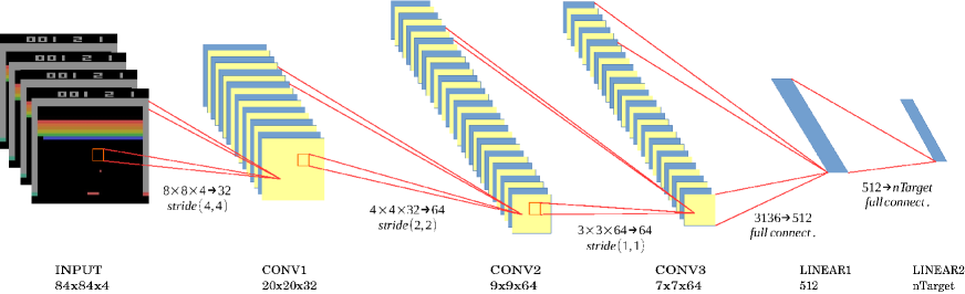
Figure 1: Architecure of Neural Network

The source code that implements the above neural network architecture is presented in the figure 3. The code uses CytonLib to build a fully operable neural network. Note that the code is slightly simplified to emphasize the working mechanism. The code works as follows,

• The class of Variable stores numeric values and gradients. Through passing the pointer of Variable around, all components are connected.

• The data member layers collects all the components. The base class of Network calls the functions forward, backward and calculateGradient of each component to perform the actual computation, illustrated by the figure 3.

Ωclass NetworkRL: public NetworkΩ{ΩConvolutionLayer conv1; // declare componentsΩActivationLayer act1;ΩConvolutionLayer conv2;ΩActivationLayer act2;ΩConvolutionLayer conv3;ΩActivationLayer act3;ΩLinearLayer lin1;ΩActivationLayer act4;ΩDueLinearLayer dueLin2;ΩLinearLayer lin2;Ω\parvoid init(Variable* x, int nTarget)Ω// x: input of the neural network which is image dataΩ// nTarget: dimension of output which equals to the number ofΩ// control signalsΩ{Ω\partx=conv1.init(tx, 32, 8, 8, 4, 4, 0, 0);Ωlayers.push_back(&conv1);Ω\partx=act1.init(tx, CUDNN_ACTIVATION_RELU);Ωlayers.push_back(&act1);Ω\partx=conv2.init(tx, 64, 4, 4, 2, 2, 0, 0);Ωlayers.push_back(&conv2);Ω\partx=act2.init(tx, CUDNN_ACTIVATION_RELU);Ωlayers.push_back(&act2);Ω\partx=conv3.init(tx, 64, 3, 3, 1, 1, 0, 0);Ωlayers.push_back(&conv3);Ω\partx=act3.init(tx, CUDNN_ACTIVATION_RELU);Ωlayers.push_back(&act3);Ω\partx=lin1.init(tx, 512, true );Ωlayers.push_back(&lin1);Ω\partx=act4.act4(tx, CUDNN_ACTIVATION_RELU);Ωlayers.push_back(&act4);Ω\parif(params.dueling)Ω{Ωtx=dueLin2.init(tx, nTarget, true);Ωlayers.push_back(&dueLin2);Ω}ΩelseΩ{Ωtx=lin2.init(tx, nTarget, true);Ωlayers.push_back(&lin2);Ω}Ω\parreturn tx; //pointer to resultΩ}Ω};Ω\end{verbatim}Ω}Ω\end{minipage}

Figure 2: Source Code of Neural Network

Ωclass LayerΩ{Ωvirtual void forward(){};Ω\parvirtual void backward(){};Ω\parvirtual void calculateGradient(){};Ω};Ω\parclass Network: public LayerΩ{Ω\parvector<Layer*> layers;Ω\parvoid forward()Ω{Ωfor(int k=0; k<layers.size(); k++)Ωlayers.at(k)->forward();Ω}Ω\parvoid backward()Ω{Ωfor(int k=layers.size()-1; k>=0; k--)Ωlayers.at(k)->backward();Ω}Ω\parvoid calculateGradient()Ω{Ωfor(int k=layers.size()-1; k>=0; k--)Ωlayers.at(k)->calculateGradient();Ω}Ω};Ω\end{verbatim}Ω}Ω\end{minipage}

Figure 3: Source Code of Network Class

The code of actual computation is organized in the functions forward, backward and calculateGradient for each type of component. The figure 3 presents some examples.

Ω\parvoid LinearLayer::forward()Ω{ΩcublasXgemm(cublasH, CUBLAS_OP_T, CUBLAS_OP_N,ΩdimOutput, num, dimInput,Ω&one, w.data, w.ni, x.data, dimInput,Ω&zero, y.data, dimOutput)Ω}Ω\parvoid LinearLayer::backward()Ω{ΩcublasXgemm(cublasH, CUBLAS_OP_N, CUBLAS_OP_N,ΩdimInput, num, dimOutput,Ω&one, w.data, w.ni, y.grad.data, dimOutput,Ω&beta, x.grad.data, dimInput));Ω}Ω\parvoid LinearLayer::calculateGradient()Ω{ΩcublasXgemm(cublasH, CUBLAS_OP_N, CUBLAS_OP_T,ΩdimInput, dimOutput, num,Ω&one, x.data, dimInput, y.grad.data, dimOutput,Ω&one, w.grad.data, w.grad.ni));Ω}Ω\par\parvoid ActivationLayer::forward()Ω{ΩcudnnActivationForward(global.cudnnHandle, activeDesc,Ω&global.one, x->desc, x->data,Ω&global.zero, y.desc, y.data) );Ω}Ω\par\end{verbatim}Ω}Ω\end{minipage}

Figure 4: Source Code of Performing Actual Computation

4 Benchmark

4.1 Settings

The hyperparameter settings of CytonRL used in the benchmarks are presented by the table 1, which are coded as the default settings. The settings are initially based on the Mnih et al. (2013); van Hasselt et al. (2015); Schaul et al. (2015); Wang et al. (2015), and modified to improve the stability and efficiency according to our experiments.

Hyperparameter	Value
Replay Memory Size	1,000,000
Input Frames	4
$\gamma$	0.99
Learning Rate	0.000625
Prioritized Exp. Replay $\alpha$	0.6
Prioritized Exp. Replay $\beta$	0.4 $\to$ 1.0 (1 $\to$ Maximum Training Step)
Train. $\epsilon$-greedy	1.0 $\to$ 0.1 (1 $\to$ 5,000,000 steps)
Test $\epsilon$-greedy	0.001
Learning Start	50,000 steps
Batch Size	32
Update Period	4 steps
TargetQ update	30,000 steps
Maximum Training Step	100,000,000 steps
Maximum Step per Episode	18,000 steps
Test Period	5,000,000 steps
Optimizer	RMSprop

Table 1: Hyperparameter Settings

4.2 Performance

The performance of CytonRL on the popular Atari game of Breakout is presented in the figure 5. CytonRL was run with four model settings as,

double DQN

: –dueling 0 –priorityAlpha 0

dueling double DQN

: –dueling 1 –priorityAlpha 0

double DQN with prioritized replay

: –dueling 0 –priorityAlpha 0.6

dueling double DQN with prioritized replay

: –dueling 1 –priorityAlpha 0.6

For echo model setting, CytonRL was trained 100,000,000 steps, and tested very 5,000,000 steps. In each test, 100 games were played, and the rewards of all games were averaged. The curves of training steps versus average test reward per game are presented in the figure.

The results reveal the strength of each model settings as dueling double DQN with prior. $\succ$ double DQN with prior. $\succ$ dueling double DQN $\succ$ double DQN. Stronger model settings tend to learn the game faster, and achieve better final performance. The results confirm that DQN, double DQN, prioritized relay, and dueling DQN are all effective RL algorithms.

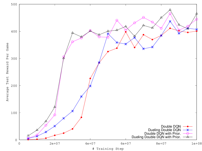
Figure 5: Performance on the Atari Game of Breakout

5 Conclusion

This paper introduces CytonRL – an open-source reinforcement learning toolkit built from scratch using C++ and NVIDA’s GPU-accelerated libraries. CytonRL is coded and tuned to achieve competitive performances in a fast manner. In other words, the toolkit is both effective and efficient. The source code of CytonRL is simple because of CytonLib – an open-source general purpose neural network library – which is contained in the toolkit. Therefore, CytonRL is an attractive alternative choice for the research community. We open-source this toolkit in the hope to benefit the community and promote the field. We look forward to hearing feedback.

References

- Bellemare et al. (2013) Marc G Bellemare, Yavar Naddaf, Joel Veness, and Michael Bowling. 2013. The arcade learning environment: An evaluation platform for general agents. J. Artif. Intell. Res.(JAIR) 47:253–279.
- Dahl et al. (2012) George E Dahl, Dong Yu, Li Deng, and Alex Acero. 2012. Context-dependent pre-trained deep neural networks for large-vocabulary speech recognition. IEEE Transactions on audio, speech, and language processing 20(1):30–42.
- Farabet et al. (2013) Clement Farabet, Camille Couprie, Laurent Najman, and Yann LeCun. 2013. Learning hierarchical features for scene labeling. IEEE transactions on pattern analysis and machine intelligence 35(8):1915–1929.
- Graves et al. (2013) Alex Graves, Abdel-rahman Mohamed, and Geoffrey Hinton. 2013. Speech recognition with deep recurrent neural networks. In Acoustics, speech and signal processing (icassp), 2013 ieee international conference on. IEEE, pages 6645–6649.
- Krizhevsky et al. (2012) Alex Krizhevsky, Ilya Sutskever, and Geoffrey E Hinton. 2012. Imagenet classification with deep convolutional neural networks. In Advances in neural information processing systems. pages 1097–1105.
- LeCun et al. (1998) Yann LeCun, Léon Bottou, Yoshua Bengio, and Patrick Haffner. 1998. Gradient-based learning applied to document recognition. Proceedings of the IEEE 86(11):2278–2324.
- Mnih (2013) Volodymyr Mnih. 2013. Machine learning for aerial image labeling. Ph.D. thesis, University of Toronto (Canada).
- Mnih et al. (2013) Volodymyr Mnih, Koray Kavukcuoglu, David Silver, Alex Graves, Ioannis Antonoglou, Daan Wierstra, and Martin A. Riedmiller. 2013. Playing atari with deep reinforcement learning. CoRR abs/1312.5602.
- Mnih et al. (2015) Volodymyr Mnih, Koray Kavukcuoglu, David Silver, Andrei A Rusu, Joel Veness, Marc G Bellemare, Alex Graves, Martin Riedmiller, Andreas K Fidjeland, Georg Ostrovski, et al. 2015. Human-level control through deep reinforcement learning. Nature 518(7540):529.
- Nair and Hinton (2010) Vinod Nair and Geoffrey E Hinton. 2010. Rectified linear units improve restricted boltzmann machines. In Proceedings of the 27th international conference on machine learning (ICML-10). pages 807–814.
- Povey et al. (2014) Daniel Povey, Xiaohui Zhang, and Sanjeev Khudanpur. 2014. Parallel training of dnns with natural gradient and parameter averaging. arXiv preprint arXiv:1410.7455 .
- Schaul et al. (2015) Tom Schaul, John Quan, Ioannis Antonoglou, and David Silver. 2015. Prioritized experience replay. CoRR abs/1511.05952.
- Sermanet et al. (2013) Pierre Sermanet, Koray Kavukcuoglu, Soumith Chintala, and Yann LeCun. 2013. Pedestrian detection with unsupervised multi-stage feature learning. In Computer Vision and Pattern Recognition (CVPR), 2013 IEEE Conference on. IEEE, pages 3626–3633.
- Sutton and Barto (1998) Richard S Sutton and Andrew G Barto. 1998. Reinforcement learning: An introduction, volume 1. MIT press Cambridge.
- van Hasselt et al. (2015) Hado van Hasselt, Arthur Guez, and David Silver. 2015. Deep reinforcement learning with double q-learning. CoRR abs/1509.06461.
- Wang et al. (2018) Xiaolin Wang, Masao Utiyama, and Eiichiro Sumita. 2018. Cytonmt: an efficient neural machine translation open-source toolkit implemented in C++. CoRR abs/1802.07170.
- Wang et al. (2015) Ziyu Wang, Nando de Freitas, and Marc Lanctot. 2015. Dueling network architectures for deep reinforcement learning. CoRR abs/1511.06581.