Spin transport in long-range interacting one-dimensional chain

Abstract

We numerically study spin transport and nonequilibrium spin-density profiles in a clean one-dimensional spin-chain with long-range interactions, decaying as a power-law, $r^{-\alpha}$ with distance. We find two distinct regimes of transport: for $\alpha<1/2$, spin excitations relax instantaneously in the thermodynamic limit, and for $\alpha>1/2$, spin transport combines both diffusive and superdiffusive features. We show that while for $\alpha>3/2$ the spin diffusion coefficient is finite, transport in the system is never strictly diffusive, contrary to corresponding classical systems.

Introduction.—Be it gravity, electromagnetic force or dipole-dipole interactions, power-law interactions are ubiquitous. While sufficiently dense mobile charges are able to screen the interaction and effectively truncate its range, in many cases long-range interactions are important. A few of the notable examples in conventional condensed matter systems are nuclear spins (Alvarez et al., 2015), dipole-dipole interactions of vibrational modes (Levitov, 1989, 1990; Aleiner et al., 2011), Frenkel excitons (Agranovich, 2008), nitrogen vacancy centers in diamond (Childress et al., 2006; Balasubramanian et al., 2009; Neumann et al., 2010; Weber et al., 2010; Dolde et al., 2013) and polarons (Alexandrov and Mott, 1996). Long range interactions are also common in atomic and molecular systems, where interaction can be dipolar (Saffman et al., 2010; Aikawa et al., 2012; Lu et al., 2012; Yan et al., 2013; Gunter et al., 2013; de Paz et al., 2013), van der Waals like (Saffman et al., 2010; Schauß et al., 2012), or even of variable range (Britton et al., 2012; Islam et al., 2013; Richerme et al., 2014; Jurcevic et al., 2014).

It was rigorously established by Lieb and Robinson that generic correlations in quantum system with short-range interactions propagate within a linear “light-cone”, $t/v=x$, with a finite velocity (Lieb and Robinson, 1972). Outside this “light-cone” correlations are exponentially suppressed (Lieb and Robinson, 1972). Specifically this implies that transport in local quantum systems cannot be faster than ballistic. Lieb-Robinson bounds were shown to be saturated for generic clean (Bohrdt et al., 2017) and weakly disordered systems (Luitz and Bar Lev, 2017).

For systems with long-range interactions the result of Lieb and Robinson doesn’t hold, but was later generalized by Hastings and Koma, who showed that for $\alpha>1$, the causal region in such systems becomes at most logarithmic, $t\sim\log x$ (Hastings and Koma, 2006). This result was subsequently improved to an algebraic “light-cone”, $t\sim r^{\delta}$ for $\alpha>2$ and $0<\delta<1$ (Foss-Feig et al., 2015). A Hastings-Koma type bound was also obtained for $\alpha<1$ after a proper rescaling of time (Storch et al., 2015). While the spreading of generic correlations was numerically studied in a number of studies (Eisert et al., 2013; Hauke and Tagliacozzo, 2013; Gong et al., 2014; Buyskikh et al., 2016; Van Regemortel et al., 2016; Luitz and Bar Lev, 2018), much less is known about transport in long-range interacting systems. Some information can be gained from quadratic fermionic models with long-range hopping (Maghrebi et al., 2016), however these systems are integrable and many times show nongeneric features. The results of Ref. (Foss-Feig et al., 2015) suggest that transport in long-range systems is at most superdiffusive for $\alpha>2$, but leaves a number of important questions open: (a) Is there an $\alpha$ above which diffusion is recovered, similarly to the situation for classical Lévy flights? (Metzler and Klafter, 2000) (b) Is there an $\alpha$, below which mean-field like dynamical behavior takes place?

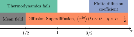
Figure 1: A cartoon describing the nature of transport in one-dimensional interacting systems, with an interaction decreasing as $r^{-\alpha}$ with the distance. For $0<\alpha<1$ the energy of the system is superextensive, resulting in the failure of conventional thermodynamics. For $0<\alpha<1/2$, dynamics corresponds to dynamics of the infinite-range $\left(\alpha\to 0\right)$ mean-field model in the limit of $L\to\infty$. For $\alpha>1/2$ transport combines diffusive and superdiffusive features.

In this work we address these questions using the time-dependent variational principle in the manifold of matrix product states (TDVP-MPS) (Verstraete et al., 2004; Haegeman et al., 2011, 2013, 2016). The main outcome of our study can be read from the cartoon in Fig. 1. TDVP-MPS belongs to the family of matrix product states (MPS) methods (Schollwöck, 2011), and thus allows to study long spin chains (chains up to $L=1,601$ were considered here), way beyond what is accessible using exact diagonalization. The main advantage of this method over the conventional time-evolving block decimation (TEBD) or time-dependent density matrix renormalization group (tDMRG) approaches for time-evolution (Vidal, 2004; White and Feiguin, 2004; Daley et al., 2004) is that the evolution is unitary by construction, and the method explicitly conserves a number of macroscopic quantities, such as the total energy, total magnetization and total number of particles (Verstraete et al., 2004; Haegeman et al., 2011, 2013, 2016). Moreover unlike TEBD and tDMRG the method can be directly applied for long-range interacting systems. While the method is numerically exact in the limit of large bond dimension (which sets the number of variational parameters), it is limited by the growth of entanglement entropy with time (Schollwöck, 2011). For a fixed bond dimension, the equations of motion of TDVP-MPS can be derived from a classical nonquadratic Lagrangian in the space of variational parameters (Haegeman et al., 2011; Leviatan et al., 2017). These equations are typically chaotic and yield diffusive transport. Based on this observation as well as the conservation properties of TDVP-MPS it was argued that the method could potentially recover correct hydrodynamic behavior also for a relatively small bond dimension (Leviatan et al., 2017), a result which was challenged in Ref. (Kloss et al., 2018). We note in passing that this line of thought is not applicable for long-range systems, where diffusive transport is not expected a-priori, and the entire hydrodynamic approach is questionable. Therefore here we strictly use TDVP-MPS as a numerically exact method.

Model.—We study a one-dimensional spin-chain of length $L$, given by the Hamiltonian $\hat{H}=\hat{H}_{\text{loc}}+\hat{H}_{\text{lr}}$ where

$$\hat{H}_{\text{loc}}=\sum_{i=1}^{L-1}\left(\hat{S}_{i}^{x}\hat{S}_{i+1}^{x}+\hat{S}_{j}^{y}\hat{S}_{i+1}^{y}\right)+\sum_{i=1}^{L-2}\left(\hat{S}_{i}^{x}\hat{S}_{i+2}^{x}+\hat{S}_{j}^{y}\hat{S}_{i+2}^{y}\right),$$ (1)

is the local part and,

$$\hat{H}_{\text{lr}}=\sum_{i=1}^{L-1}\sum_{j>i+1}^{L}\frac{1}{\left(j-i-1\right)^{\alpha}}\left(\hat{S}_{i}^{x}\hat{S}_{j}^{x}+\hat{S}_{i}^{y}\hat{S}_{j}^{y}\right),$$ (2)

includes power-law decaying long-range interactions and $\hat{S}_{i}^{x}$ and $\hat{S}_{i}^{y}$ are spin-1/2 operators. The Hamiltonian conserves the total magnetization, and thus supports energy and spin transport. In the limit of $\alpha\to\infty$, $\hat{H}_{\text{lr}}$ vanishes, and the resulting Hamiltonian corresponds to the XX ladder, which is nonintegrable and has diffusive spin transport (Steinigeweg et al., 2014; Kloss et al., 2018).

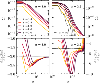
Figure 2: Upper panels. Spin excitation profiles as a function of time for two representative $\alpha$. The dashed black lines correspond to results obtained in the $\alpha\to\infty$. Darker tones represent longer times. Lower panels. Logarithmic derivative of the spin excitation profiles. The dashed black lines are guides to the eye for $2\alpha$. $L=201$, $\chi=256$ .

Method.—To assess spin transport in the system we numerically compute the two-point spin-spin correlation function at infinite temperature,

$$C_{x}\left(t\right)=\frac{4}{2^{L}}\text{Tr}\,\hat{S}_{L/2+x}^{z}\left(t\right)\hat{S}_{L/2}^{z}\left(0\right),$$ (3)

which corresponds to the time-dependent profile of a local excitation at the center of the chain performed at $t=0$. The excitation profile is obtained by propagating the operators, $\hat{S}_{i}^{z}\left(t\right),$under the Heisenberg evolution. Accessible timescales are limited by the growth of entanglement entropy during the time-evolution. Using the cyclic property of the trace $C_{x}\left(t\right)$ can be written as,

$$C_{x}\left(t\right)=\frac{4}{2^{L}}\text{Tr}\,\hat{S}_{L/2+x}^{z}\left(-\frac{t}{2}\right)\hat{S}_{L/2}^{z}\left(\frac{t}{2}\right),$$ (4)

which allows us to reach twice as large times (Kennes and Karrasch, 2016). Since we work with an approximately translationally invariant system (we use open boundary conditions), in practice, we propagate only one operator at the center of the lattice, since operators which are far enough from the boundaries of the chain can be obtained approximately by a simple translation (Sup, ). To mitigate the boundary effects introduced by this approximation we show $C_{x}\left(t\right)$ only for the central $L/2$ sites of the chain. If not stated otherwise, we use spin-chains of length $L=201$, which is sufficient to have finite size effects under control for most ranges of the interaction.

To propagate the operators we use the time-dependent variational principle (TDVP), which yields a locally optimal (in time) evolution of the wavefunction on some variational manifold. It amounts to solving a tangent-space projected Schrödinger equation (Haegeman et al., 2016),

$$\frac{d}{dt}\left|\hat{O}\left(t\right)\right\rangle=-\mathrm{i}P_{\mathcal{M}}\hat{H}\left|\hat{O}\left(t\right)\right\rangle,$$ (5)

where $P_{\mathcal{M}}$ is the tangent space projector to the variational manifold $\mathcal{M}$ and $\left|\hat{O}\left(t\right)\right\rangle$ is a vectorization of a general operator $\hat{O}\left(t\right)$. We use the matrix product operator (MPO) representation of the operator,

$$\hat{O}\left(\boldsymbol{A}\right)=\sum_{\left\{\sigma_{i}\right\},\left\{\sigma_{i}^{\prime}\right\}}A_{1}^{\sigma_{1}\sigma_{1}^{\prime}}\dots A_{N}^{\sigma_{N}\sigma_{N}^{\prime}}\left|\sigma_{1}\dots\sigma_{n}\right\rangle\left\langle\sigma_{1}^{\prime}\dots\sigma_{n}^{\prime}\right|,$$ (6)

where $\sigma_{i}=\pm 1/2$ correspond to the states of a spin at site $i$ and $A_{i}^{\sigma_{i}\sigma_{i}^{\prime}}\in\mathbb{C}^{\chi_{i-1}\times\chi_{i}}$ are complex matrices where $\chi_{i}$ is the bond-dimension of the matrix $\left(\chi_{0}=\chi_{N}=1\right)$ (Schollwöck, 2011). An exact representation of a general operator requires the bond dimension to grow exponentially with system size $L$. Therefore truncating the maximal bond-dimension to a fixed value introduces an approximation but allows to keep the MPO representation tractable. We use the family of fixed finite bond-dimension MPOs to parameterize the variational manifold, $\mathcal{M}$. Numerically exact results are achieved by convergence with respect to the bond-dimension (in this work we used bond-dimension of up to 256) (Sup, ). The evolution of (5) is performed using a second-order Trotter decomposition, with time-steps from 0.01 to 0.05. The Hamiltonian is approximated as a sum of exponentials and a short-ranged correction, which can be efficiently represented as an MPO. The number of exponentials is chosen such that the resulting couplings do not differ more than 2% from the exact couplings for any pair of sites (Crosswhite et al., 2008). We note in passing that since the evolution is unitary in the enlarged vector space of the vectorized operators and the method explicitly conserves the norm of the operator, $\left.\left\langle\hat{O}\left(t\right)\right|\hat{O}\left(t\right)\right\rangle\equiv\text{Tr}\,\hat{O}^{\dagger}\left(t\right)\hat{O}\left(t\right)=\text{Tr}\,\hat{O}^{\dagger}\hat{O}$, but not its trace, $\text{Tr}\,\hat{O}\left(t\right)$.

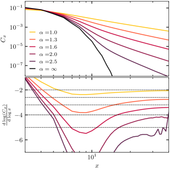
Figure 3: Upper panel. Spin excitation profiles at $t=2.0$ and various $\alpha$. Darker tones represent larger $\alpha$-s. Bottom panel. Logarithmic derivative of the spin excitation profiles. The dashed black lines are guides to the eye for $2\alpha$. $L=101$, $\chi=256$.

Results.—Figure 2 shows the spin excitation profile, $C_{x}\left(t\right)$, for short times and two values of $\alpha=1$ and $2.5.$ Since the excitation profile is symmetric with respect to the center of the lattice in the following figures we only show its right side $\left(x>0\right)$. For $\alpha=2.5$, and small distances from the initial excitation, the profile resembles a Gaussian and superimposes well with the $\alpha\to\infty$ profile calculated at same time points. For larger distances there is a crossover from a Gaussian form to a power-law form, $x^{-\gamma}$, which becomes increasingly pronounced as the time progresses. For smaller $\alpha$, the crossover is less pronounced and there is no apparent region of Gaussian behavior (although it might develop at later times). Since the accessible times in this work are short $\left(t\leq 4\right),$ due to fast growth of entanglement entropy, it is pertinent to question what our results imply on bulk transport? From Fig. 2 it is apparent that the power-law tail appears already at very short times, and its exponent $\gamma$ seems to be independent of time, as can be judged from convergence of the logarithmic derivative, $\mathrm{d}\log C_{x}\left(t\right)/\mathrm{d\log x}$, to the same value of $\gamma$ (see bottom panels of Fig. 2). This leads us to argue that the long-range nature of the interactions speeds up the approach to asymptotic transport and allows us to observe at least some of its features.

In Fig. 3 we show the spin excitation profile at $t=2$ for all analyzed $\alpha$. The power-law regime, $x^{-\gamma}$, is visible for all $\alpha$ and the exponent $\gamma\left(\alpha\right)$ is $\alpha$ dependent. To assess this dependence we calculate the corresponding logarithmic derivative (see bottom panel of Fig. 3), which converges to its asymptotic value, $\gamma$, at large distances. The logarithmic-derivative becomes increasingly noisy at large distances, $x$, (where $C_{x}\left(t\right)<10^{-8}$ ), due to decreasing signal-to-noise ratio, which prohibits us to obtain an even better convergence.

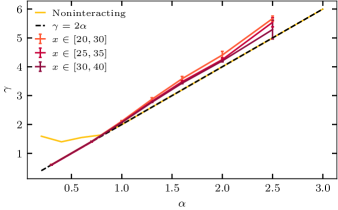
Figure 4: The power-law exponent, $\gamma$, of the power-law tail in the spin excitation profiles obtained by averaging over the logarithmic derivative in Fig. 3 in different spatial regions. The yellow (light) line is the exponent $\gamma$ computed for the noninteracting model in Eq. (7). The dashed black line corresponds to $\gamma=2\alpha$.

The Hastings-Koma bound (as also the tightened algebraic bounds) states that for $\alpha>1$, $\left\|\left[\hat{O}_{y}\left(t\right),\hat{O}_{x+y}\right]\right\|\leq c_{\alpha}\left(t\right)x^{-\alpha}$, where $\hat{O}_{i}$ are generic local operators, and $c_{\alpha}\left(t\right)$ is a constant, which depends on $t$ and $\alpha$ (Hastings and Koma, 2006). Since $C_{x}\left(t\right)$ is a correlation function, one could expect the exponent of the power-law decay of $C_{x}\left(t\right)$ to simply be $\alpha,$ namely $\gamma=\alpha$. This is however not the case as can be inferred from Fig. 4. To assess the convergence of the results we have extracted $\gamma$ by averaging the logarithmic derivative on various spatial intervals, and we note that $\gamma$ converges to the $\gamma=2\alpha$ line. We compare our results to a noninteracting long-range hopping model,

$$\hat{H}_{\text{nonint}}=\sum_{i=1}^{L}\sum_{x=1}^{L-1}\frac{1}{x^{\alpha}}\hat{c}_{i}^{\dagger}\hat{c}_{i+x},$$ (7)

where $\hat{c}_{i}^{\dagger}$ creates a spinless fermion at site $i$ (for analytical results at the groundstate, see Refs. (Vodola et al., 2014, 2015; Maghrebi et al., 2016)). Interestingly, while both models yield similar results for $\alpha>1$, they differ for $\alpha<1$, where the interacting model continues to follow the $\gamma=2\alpha$ line.

Many-times transport is characterized by considering the time-dependence of the moments of of the spin excitation profile,

$$\left\langle x^{2q}\right\rangle\left(t\right)=\sum_{x=0}^{L}x^{2q}C_{x}\left(t\right).$$ (8)

Specifically, the second moment $(q=1),$ also known as the mean-square displacement (MSD), is directly related to the the time-dependent diffusion coefficient , $D\left(t\right)=\mathrm{d}\left\langle x^{2}\right\rangle/\mathrm{d}t$, which converges to the linear response diffusion coefficient for $t\to\infty$ (see Appendix of Ref. (Luitz and Bar Lev, 2016)). Since we obtain that asymptotically $C_{x}\left(t\right)\sim x^{-2\alpha}$, all moments with $q>\alpha-1/2$ diverge in the limit $L\to\infty$. In the left panels of Fig. 5 we demonstrate this behavior for $q=1$. . While $\alpha=1.3$ shows a divergence of $D\left(t\right)$ with system size, for $\alpha=3$ the time-dependent diffusion coefficient does not depend on the system size, and approaches a plateau as a function of time, indicative of diffusive transport, $\left\langle x^{2}\right\rangle\sim Dt$. This is consistent with our observation that the central part of the excitation profile is well described by the dynamics of a local system $\left(\alpha\to\infty\right)$, which is diffusive (Steinigeweg et al., 2014; Kloss et al., 2018).

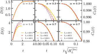
Figure 5: Left panels. Time-dependent diffusion constant $D\left(t\right)$ for $\alpha=1.3$ and $3$ and three different system sizes, $L=201,301$ and $401$, $\chi=256$. Middle and right panels. Short-time relaxation of the central spin, $C_{0}\left(t\right)$ for $\alpha=0.3$ ($C_{0}\left(5t\right)$ is plotted) and $0.7$ versus time (middle) and rescaled time (right) using the square root of the generalized harmonic numbers, $\sqrt{H_{L}^{\left(2\alpha\right)}}$ (see text) for $L=401,801$ and $1,601$ and $\chi=64$.

We note that $\alpha=1/2$ plays a special role, since for $\alpha<1/2$, $C_{x}\left(t\right)\sim x^{-2\alpha}$ becomes nonintegrable. This is in a contradiction to the fact that $\sum_{x}C_{x}\left(t\right)=\sum_{x}C_{x}\left(0\right)=1$, which follows from the conservation of total magnetization. The resolution of this apparent paradox follows from the dependence of $C_{x}\left(t\right)$ on the system size for $\alpha<1/2$, which makes the entire excitation profile (for any finite time) vanish in the limit $L\to\infty$ (Bachelard and Kastner, 2013; Kastner, 2011; van den Worm et al., 2013; Kastner, 2017). The dependence of the excitation profile on the system size for $\alpha<1/2$ can be eliminated by a proper rescaling of time, $tf\left(L\right),$ where $f\left(L\right)$ is some increasing function of $L$. We have empirically found that taking $f\left(L\right)=\sqrt{H_{L}^{\left(2\alpha\right)}}\equiv\left(\sum_{x=1}^{L}x^{-2\alpha}\right)^{1/2}$ (namely the $\ell^{2}$-norm of the long-range part) gives a perfect scaling collapse (see right panels of Fig. 5) for $\alpha<1$. In the limit of large system sizes and for $\alpha<1/2$, this rescaling corresponds to $\tau\sim tL^{1/2-\alpha}$ and is consistent with the analytically obtained rescaling for a classical model (Bachelard and Kastner, 2013; Kastner, 2017).

Summary.—Using a numerically exact method (TDVP) we study spin transport in a nonintegrable one-dimensional spin chain, with interactions which decay as $x^{-\alpha}$ with the distance. While the method allows us to address chains far beyond what is accessible using exact diagonalization, it is inherently limited to short times due to the fast growth of entanglement entropy. Nevertheless, we show, that due to the long-range of the interactions, approach to some of the asymptotic features of transport is fast enough to be observed in our simulations.

We find two pronounced regimes in the dynamics of a spin excitation. For $\alpha<1/2$, we find that the decay of the excitation depends on the system size, such that the relaxation time $t_{0}\propto\left(\sum_{k}J_{0k}^{2}\right)^{-1/2}\sim L^{\alpha-1/2}$ (where $J_{ij}\sim\left|i-j\right|^{-\alpha}$ is the long-range part of the Hamiltonian), and goes to zero in the limit of $L\to\infty$. For finite system sizes the spatial decay of the excitation profile is $C_{x}\left(t\right)\sim x^{-2\alpha}$.

For $\alpha>1/2$, there is a residual dependence of the excitation profiles on the system size, which vanishes in the $L\to\infty$ limit. For short distances the spatial excitation profiles are well described by the corresponding profiles of a local system , which for generic systems are Gaussian, corresponding to a diffusive transport. For longer distances the Gaussian form crosses-over to a power-law behavior with an exponent, which approaches, $C_{x}\left(t\right)\sim x^{-2\alpha}$. The crossover is much more apparent for larger $\alpha$, and is barely visible for the smaller $\alpha$. Our data is inconclusive with respect to the existence of a critical $\alpha_{c}>1/2$ below which the crossover vanishes, since it is possible that longer times are needed to observe the crossover for the smaller $\alpha$. The crossover point drifts to longer distances for larger $\alpha$, but we were not able to determine its precise functional dependence.

Due to the asymptotic power-law dependence of the excitation profile, only moments $\left\langle x^{2q}\right\rangle\left(t\right)$ with $q<\alpha-1/2$ exist (see Eq. 8). We find that for $\alpha>3/2$ the MSD, which corresponds to $q=1$, exists and is not system-size dependent. Moreover it appears to increase linearly with time, which we demonstrated by calculating its derivative. While this behavior corresponds to diffusion, the dynamics is not truly diffusive for any $\alpha$, due to the divergence of higher moments. This is in stark contrast to classical superdiffusive systems, such as Lévy flights, where a critical $\alpha$ exists, above which diffusion is restored. The nice agreement of the “core” of the excitation profile with a Gaussian form, corresponding to diffusion, leads us to speculate that all the existing moments have a diffusive time-dependence, namely, $\left\langle x^{2q}\right\rangle\left(t\right)\sim t^{q}$, for $q<\alpha-1/2$.

In this work we consider only one model, but due to its nonintegrability for all $\alpha$, we expect our results to hold for a broad family of nonintegrable long-range models. In particular, it would be interesting to extend our results to higher dimensions.

Supplementary material

Convergence tests.—Numerical exactness of the dynamics generated by TDVP-MPS is obtained by converging with respect to the bond-dimension, $\chi$. In Figures 6 and 7, we provide comparisons of calculations with bond-dimensions $\chi=256$ and $\chi=128$ for quantities of interest in this study. Evaluating the spatial spin excitation profile in the tails becomes sensitive to numerical noise for small values of $C_{x}$ (smaller than $10^{-8}$) and is limited by a complex interplay of time-step errors and accumulation of numerical round-off errors. Therefore, obtaining accurate tails of $C_{x}$ is harder for the large $\alpha$, where $C_{x}$ decreases faster with the distance. $\alpha=2.5$ is the shortest-ranged system for which it is possible to calculate a meaningful tail of $C_{x}$. In contrast, the mean square displacement is robust to the numerical noise in the far tails for the system sizes and times considered here, and longer times are accessible for larger $\alpha$. The relaxation of the central spin, $C_{0}(t)$, at short times is converged with a moderate bond-dimension $\chi=64$, see Fig. 8.

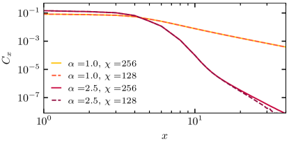
Figure 6: Convergence of the spin excitation profile with respect to bond-dimension, $\chi$, at $t=2.0$ and $L=201$.

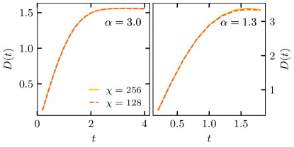
Figure 7: Convergence of the time-dependent diffusion constant $D(t)$ with respect to bond-dimension for $\alpha=1.3$ $\left(L=201\right)$ and $\alpha=3$ $\left(L=301\right)$.

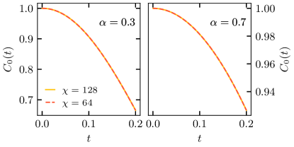
Figure 8: Convergence of the relaxation of the central spin $C_{0}(t)$ with respect to bond-dimension for $\alpha=0.3$ and $\alpha=0.7$ $\left(L=401\right)$.

Approximate evaluation of $C_{x}\left(t\right)$.—Obtaining the correlation function,

$$C_{x}(t)=\frac{1}{2^{L}}\text{Tr}\,\hat{S}_{L/2}^{z}\left(-\frac{t}{2}\right)\hat{S}_{L/2+x}^{z}\left(\frac{t}{2}\right),$$ (9)

of a spin-chain of length $L$ scales as $\mathcal{O}(L^{2})$, since for each operator, a separate calculation has to be performed. However, the scaling can be reduced to $\mathcal{O}(N)$ by making use of the approximate translational invariance of the $\hat{S}_{i}^{z}(t)$. In the limit of large system and for sites $i$ close to the center, the correlation function can be evaluated approximately using only $\hat{S}_{L/2}^{z}(t)$,

$$C_{x}\left(t\right)\approx\frac{1}{2^{L}}\text{Tr}\,\hat{S}_{L/2}^{z}\left(-\frac{t}{2}\right)\boldsymbol{T}_{x}\hat{S}_{L/2}^{z}\left(\frac{t}{2}\right),$$ (10)

where the action of the translation operator $\boldsymbol{T}_{x}$ is illustrated in Fig. 9. It can be understood as relabeling of the lattice sites $i$ in a cyclically translated manner: $\forall i\in[1,L]:i\to(i+x)\mod L$. The trace in Eq. (10) can be performed if the matrix product operator (MPO) is expanded at both ends with virtual sites connected containing identity operators and connected with a bond-dimension of 1. One may also include these sites as physical sites in the propagation, which corresponds to a mean-field description of the auxiliary sites. In this study we chose the latter and included $\frac{L}{2}$ auxiliary sites to the left and right of the chain. The system sizes $L$ reported in the main text refer to the lattice without the auxiliary sites. There is no need to evaluate $\hat{S}_{L/2}^{z}\left(-\frac{t}{2}\right)$, since it is just the complex conjugate of $\hat{S}_{L/2}^{z}\left(\frac{t}{2}\right)$. In a vectorized notation the calculation of $C_{x}\left(t\right)$ therefore amounts to the calculation of $\left\langle\hat{S}_{L/2}^{z}\left(\frac{t}{2}\right)|\boldsymbol{T}_{x}|\hat{S}_{L/2}^{z}\left(\frac{t}{2}\right)\right\rangle.$

The deviation between $C_{x}(t)$ obtained from the explicit propagation of all $\hat{S}_{x}^{z}$ and $C_{x}(t)$ calculated within this approximation is negligible for the chain lengths we use in this study, see Fig. 10. We have verified that the large errors after site 40 are not related to a breakdown of the approximate scheme, but occur due to the small signal-to-noise ratio for very small $C_{x}(t)$. For lattice sites close to the end of the chain, the approximation is expected to cause significant errors.

Figure 9: Tensor network diagram for Eq. (10). Each tensor in the network is labeled with the physical site it represents. The upper MPO corresponds to the untranslated operator $\hat{S}_{L/2}^{z}\left(-\frac{t}{2}\right)$ while the lower MPO is its translated version $\boldsymbol{T}_{3}\hat{S}_{L/2}^{z}\left(\frac{t}{2}\right)$.

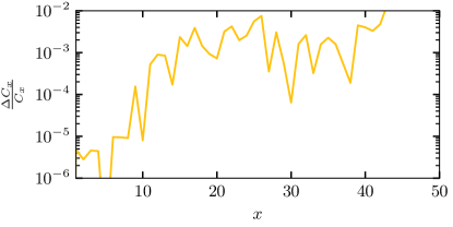
Figure 10: Relative deviation between the spin excitation profiles obtained with and without the approximation described in the text. Data shown is for $\mathrm{t=2.0,\thinspace\alpha=2.0,\thinspace dt=0.1,\thinspace\chi=128,\thinspace L=201.}$