Weak-Lensing Mass Calibration of ACTPol Sunyaev-Zel’dovich Clusters with the Hyper Suprime-Cam Survey

Abstract

We present weak-lensing measurements using the first-year data from the Hyper Suprime-Cam Strategic Survey Program on the Subaru telescope for eight galaxy clusters selected through their thermal Sunyaev-Zel’dovich (SZ) signal measured at 148 GHz with the Atacama Cosmology Telescope Polarimeter experiment. The overlap between the two surveys in this work is 33.8 square degrees, before masking bright stars. The signal-to-noise ratio of individual cluster lensing measurements ranges from 2.2 to 8.7, with a total of 11.1 for the stacked cluster weak-lensing signal. We fit for an average weak-lensing mass distribution using three different profiles, a Navarro-Frenk-White profile, a dark-matter-only emulated profile, and a full cosmological hydrodynamic emulated profile. We interpret the differences among the masses inferred by these models as a systematic error of 10%, which is currently smaller than the statistical error. We obtain the ratio of the SZ-estimated mass to the lensing-estimated mass (the so-called hydrostatic mass bias $1-b$) of $0.74^{+0.13}_{-0.12}$, which is comparable to previous SZ-selected clusters from the Atacama Cosmology Telescope and from the Planck Satellite. We conclude with a discussion of the implications for cosmological parameters inferred from cluster abundances compared to cosmic microwave background primary anisotropy measurements.

1. Introduction

Measurements of the abundance of galaxy clusters can be used as a probe of the growth of structure in the Universe. In particular, since clusters are the rarest and most massive collapsed structures, their abundances as a function of mass and redshift are particularly sensitive to the normalization of the matter power spectrum, $\sigma_{8}$, and the matter density, $\Omega_{\rm m}$ (Voit, 2005; Allen et al., 2011, for review). However, current cluster abundance measurements are limited by systematic uncertainties in observable-to-mass relations, as reported in recent measurements (e.g., Vikhlinin et al., 2009; Rozo et al., 2010; Vanderlinde et al., 2010; Sehgal et al., 2011; Benson et al., 2013; Hasselfield et al., 2013; Planck Collaboration et al., 2014b; Mantz et al., 2014; Planck Collaboration et al., 2016d; Mantz et al., 2015; de Haan et al., 2016). Thus, accurate empirical calibrations of observable-mass relations are essential for cluster surveys to fully reach their potential.

Samples of clusters are assembled based on several observables such as the density and concentration of galaxies in optical/IR observations (e.g., Rykoff et al., 2014), the projected density map measured by weak lensing (e.g., Miyazaki et al., 2018b), the X-ray emission from cluster hot gas (e.g., Pacaud et al., 2016), and the thermal Sunyaev Zel’dovich (SZ, and hereafter SZ refers to the thermal SZ) effect (Sunyaev & Zeldovich, 1969, 1972), a characteristic spectral distortion in the cosmic microwave background (CMB) induced by inverse Compton scattering between CMB photons and hot ionized electrons. The spectral shape of the SZ effect is a decrement in thermodynamic temperature at frequencies below 217 GHz and excess at higher frequencies, and its amplitude scales with the Compton-$y$ parameter. Among these observables, the SZ effect is unique because the detection efficiency is nearly independent of redshift as long as the beam size is about arcminute scale. As a consequence, SZ-selected cluster samples have well-behaved selection functions that make it straightforward to calibrate observable-to-mass relations and constrain cosmological parameters. Additionally the integrated SZ signal is a low-scatter proxy for mass (e.g., Motl et al., 2005; Nagai, 2006; Stanek et al., 2010; Battaglia et al., 2012; Sembolini et al., 2013) that is fairly robust against cluster astrophysics (e.g., Nagai, 2006; Battaglia et al., 2012; Planelles et al., 2017)

Current and recent CMB experiments like the Atacama Cosmology Telescope (ACT; Thornton et al., 2016), the South Pole Telescope (SPT; Carlstrom et al., 2011), and the Planck satellite (Planck Collaboration et al., 2016a) have provided large catalogs of SZ-selected clusters (e.g., Staniszewski et al., 2009; Marriage et al., 2011; Reichardt et al., 2013; Hasselfield et al., 2013; Planck Collaboration et al., 2014a; Bleem et al., 2015; Planck Collaboration et al., 2016b; Hilton et al., 2018). In these experiments, different observational techniques are used to measure the integrated Compton-$y$ signal and different SZ-mass scaling relations are used to infer cluster masses. For example, the Planck collaboration relies on X-ray observables for their initial calibrations of the Compton-$y$ to mass relation (Planck Collaboration et al., 2014a). However, the determination of a cluster’s total mass (including dark matter) from X-ray observables assumes that the intracluster medium is in hydrostatic equilibrium. Such physical assumptions can be a source of systematic uncertainties in cluster mass estimates (e.g., Evrard, 1990; Rasia et al., 2004; Lau et al., 2009; Battaglia et al., 2012; Nelson et al., 2012; Rasia et al., 2012).

The technique of weak lensing offers direct measurement of the total matter distribution of a galaxy cluster (baryonic and dark matter), and can thus provide an unbiased mass calibration. Weak lensing manifests itself as small but coherent distortions of distant galaxies that result from the gravitational deflection of light due to foreground structures (e.g., Kaiser, 1992). Cluster weak lensing appears as tangential shear of background galaxy shapes around a cluster. Numerous attempts to calibrate SZ masses have been made in the literature using ACT clusters (Miyatake et al., 2013; Jee et al., 2014; Battaglia et al., 2016), SPT clusters (McInnes et al., 2009; High et al., 2012; Schrabback et al., 2016; Dietrich et al., 2017; Stern et al., 2018), Planck clusters (von der Linden et al., 2014b; Hoekstra et al., 2015; Penna-Lima et al., 2017; Sereno et al., 2017; Medezinski et al., 2018a), Planck and SPT clusters (Gruen et al., 2014), and other massive cluster samples (Marrone et al., 2009; Hoekstra et al., 2012; Marrone et al., 2012; Smith et al., 2016). The mass calibration is often parametrized as

$$1-b=\frac{M_{\rm SZ}}{M_{\rm true}},$$ (1)

where $M_{\rm SZ}$ is the SZ mass and $M_{\rm true}$ is the true cluster mass, which for this paper we take to be the weak-lensing mass $M_{\rm WL}$. This ratio can be taken for individual clusters or for an ensemble average and these values will be consistent as long as the appropriate weights are used (Medezinski et al., 2018a). Recently, Planck Collaboration et al. (2016d) reported a disagreement between $1-b$ obtained by weak-lensing calibrations of Planck SZ cluster masses (e.g., von der Linden et al., 2014b; Hoekstra et al., 2015) and that inferred from reconciling the Planck primary CMB parameters with the Planck SZ cluster counts. This disagreement is not statistically significant ($\sim 2\sigma$) and will decrease after accounting for additional bias corrections, like Eddington bias (Battaglia et al., 2016) and new optical depth measurements (Planck Collaboration et al., 2016e). However, if such a disagreement persists as the precision of cluster measurements improves, then it could reveal the need for extensions to the standard cosmological model (Planck Collaboration et al., 2016c), like a non-minimal sum of neutrino masses (e.g., Wang et al., 2005; Shimon et al., 2011; Carbone et al., 2012; Mak & Pierpaoli, 2013; Louis & Alonso, 2017; Madhavacheril et al., 2017), or illuminate additional systematic effects in cluster abundance measurements.

In this paper, we present weak-lensing mass calibrations of SZ-selected clusters. We perform weak-lensing measurements using Subaru Hyper Suprime-Cam (HSC) Strategic Survey Program (SSP) data (Aihara et al., 2018a). The SZ cluster sample is based on the ACT Polarimeter (ACTPol) two-season cluster catalog (Hilton et al., 2018). Section 2 describes the details of the ACTPol data and HSC data used in these measurements. Section 3 describes the details of the weak-lensing measurements, including our investigation of systematics. Section 4 presents the mass calibration of SZ clusters, and we discuss our results and conclude in Section 5. Throughout the paper, we adopt the flat-$\Lambda$CDM cosmology with $\Omega_{m}=0.3$ and $h=0.7$. The SZ masses are quoted in $M_{\rm 500c}$ where the mass enclosed in $R_{\rm 500c}$ is 500 times the critical density of the Universe at the redshift of the cluster. Some of the weak-lensing masses are defined by $M_{\rm 200m}$ where the mass enclosed in $R_{\rm 200m}$ is 200 times the mean matter density. When this is true we converted $M_{\rm 200m}$ to $M_{\rm 500c}$ to compare to the SZ mass.

2. Data

2.1. ACTPol Clusters

The cluster sample used in this work is drawn from the ACTPol two-season cluster catalog (Hilton et al., 2018). The sample was extracted from 148 GHz observations of a 987.5 deg² equatorial field that combined data obtained using the original ACT receiver (MBAC; Swetz et al., 2011) with the first two seasons of ACTPol data. Details of the ACTPol observations and map making can be found in Naess et al. (2014) and Louis et al. (2017). Cluster candidates were detected by applying a spatial matched filter to the map, using the Universal Pressure Profile (UPP; Arnaud et al., 2010) and its associated SZ signal-mass scaling relation to model the cluster signal. Candidates were then confirmed as clusters and their redshifts measured using optical/IR data, principally from the Sloan Digital Sky Survey (SDSS DR13; Albareti et al., 2017). Cluster masses were estimated by applying the Profile Based Amplitude Analysis technique, introduced in Hasselfield et al. (2013). In this paper, we use $M_{\rm SZ}$ to refer to SZ-based mass estimates that correspond with $M^{\rm UPP}_{\rm 500c}$ as tabulated in Hilton et al. (2018). The full cluster sample in Hilton et al. (2018) are all signal-to-noise $(S/N)>4$ with mass range of roughly $2\times 10^{14}\,$M${}_{\odot}<M_{\rm SZ}<9\times 10^{14}\,$M_⊙ with a median mass of $M_{\rm SZ}=3.1\times 10^{14}\,$M_⊙ and redshift range of roughly $0.15<z<1.4$ with a median redshift of $z=0.49$.

2.2. HSC - ACT Survey Overlap

Among the HSC first-year data (Aihara et al., 2018b), the XMM field in the HSC Wide Layer overlaps with the deepest region of the ACTPol maps - the D6 field at 02^h30^m RA (Naess et al., 2014; Louis et al., 2017). The sample studied in this work consists of ACTPol clusters in this region that were detected with SNR${}_{\rm 2.4}>5$ in the Hilton et al. (2018) catalog, where SNR_2.4 refers to the signal-to-noise ratio of the cluster, as measured in a map filtered at an angular scale of 2.4$\arcmin$ (refer to Sections 2.2 and 2.3 of Hilton et al. 2018 for details). Above this threshold, the cluster sample in the HSC S16A region is 100% pure with complete redshift follow-up.

Figure 1 shows the 90% mass completeness limit as a function of redshift across the HSC S16A region, using the UPP model and associated scaling relation to convert the SZ signal into mass, as described in Section 2.4 of Hilton et al. (2018). Averaged over $0.2<z<1$, the sample is 90% complete for $M_{\rm SZ}>3.2\times 10^{14}$ M_⊙. This is significantly lower than the equivalent limit of $M_{\rm SZ}>4.5\times 10^{14}$ M_⊙ obtained when averaging over the whole 987.5 deg² ACTPol field, since the overlapping HSC S16A region lies in a low noise region of the ACTPol survey D6 (see Naess et al., 2014).

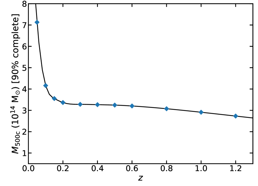
Figure 1.— Survey-averaged 90% $M_{\rm SZ}$ completeness limit as a function of redshift, using the UPP and Arnaud et al. (2010) mass scaling relation to model the SZ signal, estimated in the HSC S16A region. The blue diamonds mark the redshifts at which the limit was estimated, and the solid line is a cubic spline fit. In the redshift range $0.2<z<1.0$, the average 90% completeness limit is $M_{\rm SZ}>3.2\times 10^{14}$ M_⊙ for SNR${}_{2.4}>5$.

Figure 2 shows the overlap between the ACTPol D6 field and the HSC XMM field. There are eight clusters that span a redshift range of $0.186\leq z\leq 1.004$. The average cluster redshift, which is weighted by the source galaxy weight described in Section 3.1, is $\langle z_{l}\rangle=0.43$.

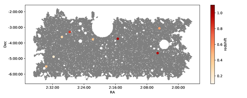
Figure 2.— ACTPol SZ-selected clusters in the HSC XMM field. The colored points show the eight ACTPol clusters with the redshift information. The gray points are HSC source galaxies used for our lensing analysis, which covers $29.5$ deg². Note that holes in the source galaxy distribution are due to the bright star mask.

Table 1 lists the properties of the sample. When measuring the shear signal from the HSC data, we define the cluster centers as the brightest cluster galaxy (BCG) locations as determined by Hilton et al. (2018) using a combination of visual inspection and the $i$, $r-i$ color-magnitude diagram. We match the ACTPol clusters with optically-selected clusters in the HSC Wide S16A data set by the CAMIRA algorithm in Oguri et al. (2018), requiring separation $<2^{\prime}$. The optical richness derived by CAMIRA, $N_{\mathrm{cur}}$, is shown in Table 1. Figure 3 shows the HSC color images of our sample together with the SZ $S/N$ contours. The cluster centers which are defined by the BCG and SZ signals are consistent for most of the clusters, given that the beam of ACTPol is about $1.4\arcmin$ at 148 GHz. Only ACT-CL J0229.6-0337 has a significantly large offset between these cluster centers. We will look into how the offset affects our lensing signal in Appendix B.3.

Table 1ACTPol clusters overlapping with the HSC XMM field.

Name	SZ RA	SZ Dec	BCG RA	BCG Dec	Redshift1	SNR2.4	$M_{\rm SZ}$ [1014M⊙]	$N_{\rm cor}$2
ACT-CL J0204.8-0303	2:04:49.73	-3:03:38.42	2:04:50.27	-3:03:36.82	0.549	6.84	3.04${}^{+0.57}_{-0.48}$	35.0
ACT-CL J0205.2-0439	2:05:15.90	-4:39:07.50	2:05:16.69	-4:39:19.96	0.968	8.10	3.12${}^{+0.52}_{-0.44}$	38.6
ACT-CL J0215.3-0343	2:15:23.72	-3:43:45.20	2:15:24.01	-3:43:31.98	1.004	5.86	2.46${}^{+0.44}_{-0.37}$	44.8
ACT-CL J0221.7-0346	2:21:44.53	-3:46:19.94	2:21:45.17	-3:46:02.19	0.432	7.29	3.07${}^{+0.59}_{-0.50}$	69.3
ACT-CL J0227.6-0317	2:27:37.77	-3:17:53.48	2:27:38.22	-3:17:57.31	0.838	5.15	2.19${}^{+0.42}_{-0.35}$	50.9
ACT-CL J0229.6-0337	2:29:36.88	-3:37:04.01	2:29:43.97	-3:36:53.52	0.323	5.15	2.40${}^{+0.54}_{-0.44}$	57.0
ACT-CL J0231.7-0452	2:31:43.63	-4:52:56.16	2:31:41.17	-4:52:57.44	0.186	6.85	3.08${}^{+0.72}_{-0.58}$	116.4
ACT-CL J0233.6-0530	2:33:36.27	-5:30:34.52	2:33:35.59	-5:30:21.76	0.435	6.91	3.11${}^{+0.61}_{-0.51}$	46.9
1 Redshifts are spectroscopic measurements.
2 Richness is from the HSC CAMIRA cluster catalog (Oguri et al., 2018).

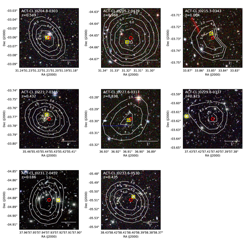
Figure 3.— ACTPol SZ-selected clusters observed by HSC S16A wide XMM field. The images of clusters with $z>0.6$ are composed of $izy$-bands and the others are $riz$-bands. Red circles denote the SZ centers, and yellow squares denote the BCG centers. White contours show the SZ $S/N$ in units of $\sigma$ for the mm-wave detection. The distorted contours of ACT-CL J0215.3-0343 are due to a point-source mask.

2.3. HSC Source Galaxies

HSC is the wide-field prime focus camera on the Subaru Telescope (Miyazaki et al., 2018a; Komiyama et al., 2018) located at the summit of Mauna Kea. The combination of the wide field-of-view (1.77 deg²), superb image quality (seeing routinely less than $0.6^{\prime\prime}$), and large aperture of the primary mirror (8.2 m) makes HSC one of the best instruments for conducting weak-lensing cosmology. Under the Subaru Strategic Survey Program (SSP; Aihara et al., 2018a), HSC started a galaxy imaging survey in 2014 that aims to cover 1,400 deg² of the sky down to $i=26$ after its 5 years of operation. The first-year galaxy shape catalog (Mandelbaum et al., 2018) was produced using the data taken from March 2014 through April 2016 with about 90 nights in total. The first-year data consists of six distinct fields (HECTOMAP, GAMA09H, WIDE12H, GAMA15H, XMM, VVDS) and covers $136.9$ deg² in total. Note that this catalog is a slight extension of Data Release 1 (Aihara et al., 2018b). As mentioned above, we use the shape catalog in the XMM field ($29.5$ deg² once we remove the star mask region) which overlaps with the current ACTPol observations. The weighted number density of source galaxies in this field is 22.1 arcmin^-2 and their median redshift is $z_{\rm m}=0.82$.

Here we briefly summarize the HSC shape catalog. For details of the shape catalog production, see Mandelbaum et al. (2018). The galaxy shapes were estimated on coadded $i$-band images by the re-Gaussianization technique (Hirata & Seljak, 2003), which is a moment-based method with PSF correction. This method was extensively used and characterized in the Sloan Digital Sky Survey (Mandelbaum et al., 2005; Reyes et al., 2012; Mandelbaum et al., 2013). The shapes $(e_{1},e_{2})=(e\cos 2\phi,e\sin 2\phi)$, where $\phi$ is position angle, are defined in terms of distortion, $e=(a^{2}-b^{2})/(a^{2}+b^{2})$, where $a$ and $b$ are the major and minor axes, respectively (Bernstein & Jarvis, 2002). The galaxy shapes were calibrated against image simulations generated with GalSim (Rowe et al., 2015), an open source software package, which yields correction factors for the shear measurements. These factors are the multiplicative bias $m$ and additive bias $(c_{1},c_{2})$, which are defined as $g_{i,\rm{obs}}=(1+m)g_{i,\rm{true}}+c_{i}$, where $(g_{1},g_{2})$ is defined in terms of shear, $g=(a-b)/(a+b)$, and must be applied to the shear measurements. Note that the multiplicative bias is shared between the two ellipticity components (for details, see Mandelbaum et al., 2017). For each galaxy, the shape catalog provides an estimate of the intrinsic shape noise, $e_{\rm rms}$, an estimate of measurement noise, $\sigma_{e}$, and inverse weights $w$ from combining $e_{\rm rms}$ and $\sigma_{e}$. The measurement noise is statistically estimated from the shape measurements performed on simulated images, and the intrinsic shapes are derived by subtracting the measurement noise from the ellipticity dispersion measured from the real data. Note that we use a catalog made with the “Sirius” star mask, which actually includes bright galaxies and thus an extended region around each BCGs may be masked as well. After we performed the lensing measurement, the shape catalog was updated with a more reliable star mask called “Arcturus” (for details, see Coupon et al., 2018). We checked that switching to this new shape catalog changes our fiducial stacked weak-lensing measurements by an amount well within the statistical uncertainty (typically 10 %).

We use photometric estimates to select source galaxies based on colors. For this purpose, we use cmodel magnitudes derived by fitting a galaxy’s light profile with a composite model of the exponential and de Vaucouleurs profile (Bosch et al., 2018). The HSC SSP catalog has photo-$z$ estimates based on six different methods (Tanaka et al., 2018). Among these methods, we use MLZ, an unsupervised machine learning method based on the Self-Organizing Map which is a projection map from multi-dimensional color space to redshift, for our fiducial measurement. We have checked the consistency among lensing signals with different photo-$z$ methods, which is described in Appendix B.2. In this paper, we use the redshift PDFs, $P(z)$, and randomly sampled point estimates that are drawn from the PDFs, $z_{\rm mc}$. The latter is specifically used for one of the source galaxy selection methods described below.

3. Weak-Lensing Measurements

In this section, we describe basics of weak lensing measurement in Section 3.1, covariance estimation in Section 3.2, and key systematic tests, i.e., source galaxy selection and photo-$z$ bias in Sections 3.3 and 3.4. Additional systematic tests we performed are described in Appendix B.

3.1. Weak Lensing Basics

Weak gravitational lensing manifests as a coherent distortion of apparent shapes of source galaxies. For a source galaxy at a comoving transverse separation $R$ from the lens center, the lens’ gravitational potential induces a tangential distortion, $\gamma_{t}$, which depends on the lens’ matter density profile projected along the line of sight, $\Sigma(R)$, and on the redshifts of the source galaxy, $z_{s}$, and the lens, $z_{l}$. For the purposes of this work the lenses are galaxy clusters. In terms of the average projected mass density inside $R$, $\bar{\Sigma}(<R)$, and the critical surface mass density $\Sigma_{cr}(z_{l},z_{s})$ defined below, the tangential distortion can be expressed in terms of the excess surface mass density $\Delta\Sigma(R)$ as follows:

$$\gamma_{t}(R)=\frac{\bar{\Sigma}(<R)-\Sigma(R)}{\Sigma_{\rm cr}(z_{l},z_{s})}\equiv\frac{\Delta\Sigma(R)}{\Sigma_{\rm cr}(z_{l},z_{s})}.$$ (2)

In terms of the angular diameter distances of the source and lens from us, $D_{A}(z_{s})$ and $D_{A}(z_{l})$, and the angular diameter distance between the two, $D_{A}(z_{s},z_{l})$, $\Sigma_{\rm{cr}}(z_{s},z_{l})$ is defined as:

$$\Sigma_{\mathrm{cr}}(z_{l},z_{s})=\frac{c^{2}}{4\pi G}\frac{D_{A}(z_{s})}{(1+z_{l})^{2}D_{A}(z_{l})D_{A}(z_{l},z_{s})}.$$ (3)

where the factor $(1+z_{l})^{-2}$ comes from our use of comoving coordinates (Mandelbaum et al., 2006).

To estimate cluster properties including mass from measurements of $\Delta\Sigma$, we will start with models of the cluster density radial profile, $\rho(r)$, and integrate to generate modeled lensing profiles $\Delta\Sigma(r;M,x)$, where $x$ signifies other possible parameters of the models (see Section 4). From the data, we can estimate $\Delta\Sigma$ in each radial bin $R_{i}$ for either a single cluster or a stack of multiple clusters with a weighted sum over the tangential components of the shapes of galaxies, $e_{t}$, as follows. We use a weighting based both on the shape catalog weight for the source galaxy, $w_{s}$, and on an estimate of the appropriate critical surface mass density for the particular source-lens pair, using the photo-$z$ PDF for each source, $P_{s}(z)$, to account for the dilution effect of foreground galaxies. (See Section 3.3 for discussion of the impact of possible cluster member contamination, however.) Specifically, we define $\tilde{w}_{ls}\equiv w_{s}\langle\Sigma_{cr,ls}^{-1}\rangle^{2}$, where

$$\left\langle\Sigma_{{\rm cr},ls}^{-1}\right\rangle=\frac{\int_{0}^{\infty}P_{s}(z_{s})\Sigma_{{\rm cr}}^{-1}(z_{l},z)dz}{\int_{0}^{\infty}P_{s}(z)dz}.$$ (4)

With two additional calibration factors described below, the lensing profile is estimated as:

$$\Delta\Sigma(R_{i})=\frac{1}{{2\cal R}(R_{i})}\frac{\sum_{ls\in R_{i}}\tilde{w}_{ls}e_{t,ls}\left\langle\Sigma_{{\rm cr},ls}^{-1}\right\rangle^{-1}}{(1+K(R_{i}))\sum_{ls\in R_{i}}\tilde{w}_{ls}}.$$ (5)

The factor $1+K(R)$ is the shear calibration factor which corrects for multiplicative bias described in Section 2.3;

$$1+K(R_{i})=\frac{\sum_{ls\in R_{i}}\tilde{w}_{ls}\left(1+m_{s}\right)}{\sum_{ls\in R_{i}}\tilde{w}_{ls}},$$ (6)

where $m_{s}$ is the multiplicative bias of the source, $s$. The shear responsivity ${\cal R}(R_{i})$ is necessary to take into account the summation in non-Euclidean shear space. It is calculated as

$${\cal R}(R_{i})=1-\frac{\sum_{ls\in R_{i}}\tilde{w}_{ls}e_{{\rm rms},ls}^{2}}{\sum_{ls\in R_{i}}\tilde{w}_{ls}}.$$ (7)

We compute $\Delta\Sigma$ in 12 logarithmic bins from 0.1 $\>h^{-1}{\rm{Mpc}}$ to 10 $\>h^{-1}{\rm{Mpc}}$. Note that we do not use all the radial bins for model fitting, as described later.

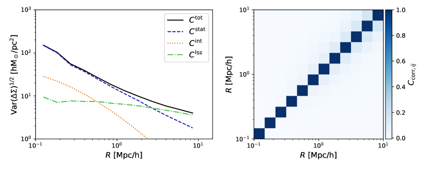
Figure 4.— Left: Diagonal components of the covariance matrix used in the stacked analysis. The black solid curve denotes the total covariance; the blue dashed curve denotes the statistical uncertainty due to intrinsic shapes of source galaxies, the orange dotted line denotes the covariance due to intrinsic variations of cluster properties such as triaxiality and concentration, and the green dashed-dotted line denotes the covariance due to large scale structure uncorrelated with clusters. Shape noise is dominant for $r<2.8\>h^{-1}{\rm{Mpc}}$, while the large-scale structure covariance dominates at larger separations. Right: The stacked analysis correlation matrix of the total covariance as a function the radial bin. The correlation between radial bins appears at large scales due to the large scale structure covariance.

3.2. Covariance

We estimate the covariance matrix of the lensing signal as

$$C=C^{\rm stat}+C^{\rm int}+C^{\rm lss},$$ (8)

where $C^{\rm stat}$ is the statistical uncertainty due to galaxy shapes:

$$C^{\rm stat}_{ij}=\frac{1}{4{\cal R}^{2}(R_{i})}\frac{\sum_{ls\in R_{i}}\tilde{w}^{2}_{ls}(e^{2}_{{\rm rms},ls}+\sigma_{e,ls}^{2})\left\langle\Sigma_{{\rm cr},ls}^{-1}\right\rangle^{-2}}{\left[1+K(R_{i})\right]^{2}\left[\sum_{ls\in R_{i}}\tilde{w}_{ls}\right]^{2}}\delta_{ij};$$ (9)

$C^{\rm int}$ accounts for the intrinsic variations of projected cluster mass profiles such as halo triaxiality, the presence of correlated halos, and the intrinsic scatter of the concentration–mass relation (Gruen et al., 2015); and $C^{\rm lss}$ is due to uncorrelated large scale structure (LSS) along the line of sight. Detailed calculations of the intrinsic and LSS covariances are described in Appendix A. Figure 4 shows the diagonals of the covariance matrix used in our analysis and the correlation matrix, defined as $C_{{\rm corr},ij}=C_{ij}/\sqrt{C_{ii}C_{jj}}$. A similar figure was presented in Umetsu et al. (2016), which describes a joint weak and strong lensing analysis of 20 high-mass clusters. Figure 4 shows that the total uncertainty is dominated by the shape noise ($C^{\rm stat}$) at $r\lower 3.01385pt\hbox{$\;\buildrel<\over{\sim}\;$}3$ Mpc $h^{-1}$, beyond which the relative contribution from LSS noise, uncorrelated with the cluster, becomes important.

3.3. Source Galaxy Selection

If cluster galaxies are misidentified as background galaxies, they will introduce a systematic dilution of the weak-lensing signal from their galaxy cluster. We look into two distinct source galaxy selection methods which were established in Medezinski et al. (2018b) with the CAMIRA catalog of optically-selected clusters in HSC SSP: a selection based on the color-color space (the CC cut) and another based on a cumulative photo-$z$ PDF (the $P(z)$ cut). Note that we use MLZ to define the latter cut and calculate lensing signals.

The CC cut is defined in the $g-i$ vs $r-z$ space to minimize the dilution in lensing signal due to the contamination by cluster members and foreground galaxies. The CC cut is defined differently for a cluster with $z_{l}\leq 0.4$ and $z_{l}>0.4$ to avoid excessively removing galaxies behind low redshift clusters (for the detailed definition, see Appendix A in Medezinski et al. 2018b). Using the CC cut Medezinski et al. 2018b showed that the dilution is consistent with zero.

The $P(z)$ cut initially proposed in Oguri (2014) is defined by two criteria that each galaxy must satisfy to be identified as a background galaxy. The first criterion is

$$p_{\rm cut}<\int_{z_{\rm min}}^{\infty}P(z){\rm d}z,$$ (10)

where $p_{\rm cut}=0.98$, meaning that we require that 98% of the area beneath the $P(z)$ lies beyond $z_{\rm min}$. For our analysis $z_{\rm min}=z_{l}+\Delta z$ and we employ $\Delta z=0.2$ for a secure rejection of cluster galaxies, following the investigation by Medezinski et al. (2018b). The second criterion is that each galaxy’s randomly drawn point redshift value from its photo-z PDF, $z_{\rm mc}$, be less than $z_{\rm max}$. This criterion rejects photo-z PDFs that are predominantly above the redshift limit that are considered secure for a given optical survey. This maximum redshift is optimized for HSC and set to $z_{\rm max}=2.5$ (see Medezinski et al., 2018b).

Figure 5 compares the stacked lensing signal from the eight clusters in the sample calculated without source selection cuts, with CC cuts, and with P(z) cuts. We do not find a significant difference among these signals within the error bars. Following the extensive analysis in Medezinski et al. (2018b) that found the CC cuts to be less diluted, we use the CC cut for our fiducial measurement.

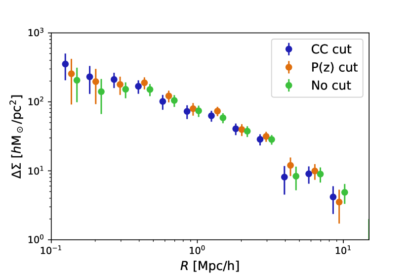
Figure 5.— The stacked weak-lensing signal from the eight clusters in the sample for different source galaxy selection methods to test the contamination from galaxies physically associated with clusters. The data points with the $P(z)$ cuts and no cuts are shifted along the x-axis for illustrative purposes. The CC cut denotes the selection in the color-color space detailed in Medezinski et al. (2018b), while the $P(z)$ cut is based on Oguri (2014) with some tweaks. We also show the signal without any source selection. The dilution effects due to contamination by foreground galaxies are already corrected for because of our use of full photo-$z$ PDF in the calculation of critical surface mass density (see Eq. 4). We use the CC cut for our fiducial measurement.

3.4. Photo-$z$ Biases

Systematic biases in the photometric redshift estimates of source galaxies would propagate to the weak lensing signal measurement through the calculation of the critical surface density. Following Mandelbaum et al. (2008), this bias in the weak lensing signal of a cluster at redshift $z_{l}$ can be estimated as

$$\frac{\Delta\Sigma}{\Delta\Sigma^{\rm true}}(z_{l})=1+b(z_{l})=\frac{\sum_{s}\tilde{w}_{ls}\langle\Sigma_{{\rm cr},ls}^{-1}\rangle^{-1}[\Sigma_{{\rm cr},ls}^{\rm true}]^{-1}}{\sum_{s}\tilde{w}_{ls}}\,,$$ (11)

where the quantities with a superscript ”true” denote the quantity as would be measured with a spectroscopic sample, the sum over $s$ goes over all source galaxies.

Nominally such photo-z biases are evaluated using a spectroscopic redshift (spec-$z$) sample that is independent from those used to calibrate the photometric redshifts and has the same population properties (magnitude and color distribution) as our source redshift sample. In practice it is difficult to obtain such a representative spec-$z$ sample given the depth of our source catalog. In principle the difference among the populations of an existing spec-$z$ sample and the weak lensing source sample can be accounted for by using a clustering and reweighting technique (for assumptions and caveats of this method, see Bonnett et al., 2016; Gruen et al., 2017). This method decomposes galaxies in the source sample into groups with similar properties. Then the galaxies from the spectroscopic sample in these groups are reweighted to mimic the distribution of the weak lensing source sample.

The first-year HSC shape catalog has substantial overlaps with public spec-$z$ samples, such as GAMA and VVDS, however, they are not enough galaxies with spec-z to represent the source sample even after reweighting. Instead of the spec-$z$ sample we use the COSMOS-30 band photo-$z$ (Ilbert et al., 2009) sample. We decompose the galaxies in the weak lensing sample using their $i$ band magnitude and 4 colors into cells of a self-organizing map (SOM, More S. et al., in prep.). Using the HSC photometry of the COSMOS 30-band photo-$z$ sample, we classify them into SOM cells defined by the source galaxy sample and compute their new weights ($w_{\rm SOM}$) which adjusts the COSMOS 30-band photo-$z$ sample to mimic our source galaxy sample. We compute the photo-$z$ bias (see Eq. 11) by including $w_{\rm SOM}$ in the definition of $w_{ls}$. Then we average Eq. 11 over our cluster sample with the weight defined by Eq. 23 in Nakajima et al. (2012). This yields a two percent bias which negligible compared to statistical uncertainties.

4. Results

4.1. Individual Cluster Measurements

In Figure 6, we show the lensing signal, $\Delta\Sigma$, for each cluster in our sample. We estimate properties for each cluster using the Navarro-Frenk-White (NFW) radial density profile (Navarro et al., 1996, 1997):

$$\rho_{{}_{\rm NFW}}(r)=\frac{\rho_{s}}{(r/r_{s})(1+r/r_{s})^{2}}.$$ (12)

Following Okabe et al. (2010), we convert the parameterization of $\rho_{{}_{\rm NFW}}$ from characteristic density and scale, $\rho_{s}$ and $r_{s}$, to mass $M_{200m}$, and concentration, defined as $c_{200m}\equiv R_{200m}/r_{s}$. We integrate the 3D $\rho_{{}_{\rm NFW}}$ to generate the fitting function $\Delta\Sigma($R$;M_{200m},c_{200m})$ and fit for both parameters. We restrict the fitting range to $0.3\>h^{-1}{\rm{Mpc}}<R<3\>h^{-1}{\rm{Mpc}}$, where the lower limit is to avoid using blended images as blending is more prominent towards the cluster center (Medezinski et al., 2018b), and the upper limit is to avoid the fitting being affected by the 2-halo regime (Applegate et al., 2014). We use only shape noise for this fitting, since the other components are negligible at these scales (see Figure 4). The constraint on the enclosed mass and concentration are then converted to $M_{\rm 500c}$ and $c_{\rm 500c}$, as shown in each panel of Figure 6 along with the signal-to-noise ratio for the weak-lensing measurement and the cluster redshift. The three high-redshift clusters, ACT-CL J0205.2-0439, ACT-CL J0215.3-0343, and ACT-CL J0227.6-0317, have low signal-to-noise ratios which are reflected in their poor best fit curves and their weakly constrained lensing mass and concentration.

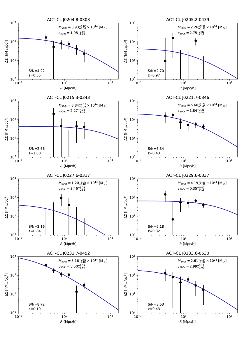
Figure 6.— The weak-lensing signals for individual clusters. The blue solid curves denote the best-fit NFW profile for which we use data points in the radial range of $0.3\>h^{-1}{\rm{Mpc}}<R<3\>h^{-1}{\rm{Mpc}}$. The median and 68% confidence levels of $M_{\rm 500c}$ and $c_{\rm 500c}$ are show in the upper right of each panel. The signal-to-noise ratio of the lensing measurement and the cluster redshift are shown in the lower left.

4.2. Stacked Cluster Measurement

We obtain the stacked cluster lensing signal (Equation 5) with a signal-to-noise ratio of $11.1$ ($9.6$ for the data used for mass inference, see below). Our goal is to estimate the average mass of the clusters in the stack to compare to the average $M_{SZ}$. We introduce an improved method for estimating the average mass in Section 4.2.2, focusing on two models for the density profiles, as described below. For comparison with earlier work, in Section 4.2.1 we also estimate the average mass with the single-mass-bin fit, which is done using only the stacked cluster signal, fitted with a model parameterized by a single mass.

The single-mass-bin fit has been widely performed in the literature, but is limited by the fact that the amplitude of the lensing signal is not linearly proportional to the cluster mass. Our method improves upon it by emulating the stacking process and incorporating the effects of the cluster mass function and selection function.

For estimating the average cluster mass, we use the “Dark Emulator” model and the “Baryonic Simulations” model described in the next few paragraphs. We also present results from the NFW density profile for comparison to earlier work. Both these models provide excess surface density profiles up to the two-halo regime, allowing use of the large scale information to constrain halo mass. Thus, we extend the fitting range up to $10h^{-1}$ Mpc for those models, rather than the $3h^{-1}$ Mpc limit for the NFW fit, which results in tighter constraints on cluster mass.

The Dark Emulator model is based on a cosmic emulator developed by Nishimichi et al. (in prep.) and it predicts statistical quantities of halos, including the mass function, the halo-matter cross-correlation, and the halo autocorrelation, as a function of halo mass, redshift, and cosmological model. The Dark Emulator model is based on a large set of $N$-body simulations; details can be found in Murata et al. (2017). We convert $M_{200m}$ to $M_{500c}$ assuming the NFW profile with $c_{200m}$ derived by Diemer & Kravtsov (2015). To compute the concentration and conversion, we use the public, open source software called Colossus (Diemer, 2017).

The Baryonic Simulations model is based on hydrodynamical simulations of cosmological volumes described in Battaglia et al. (2010). From these simulations we project the mass distributions of the halos in all the simulation snapshots at given redshifts following the methodology in Battaglia et al. (2016).

4.2.1 Single Mass-bin Fit

The results of the single-mass-bin fits are summarized in Table 2 and the model fits compared to measurements are shown in Figure 7. When fitting the NFW profile, we again vary both $M_{200m}$ and $c_{200m}$. We assume all the clusters are at a single redshift, which we calculate as a weighted average over the lens-source pairs used in the stacked measurement: $\langle z_{l}\rangle_{{\rm stack}}=\sum_{ls}\tilde{w}_{ls}z_{l}/\sum_{ls}\tilde{w}_{ls}=0.43.$ For the Baryonic Simulations model, we average the calculated excess surface density profile as a function of mass in the three redshift outputs that are closest to the value $\langle z_{l}\rangle_{{\rm stack}}$. As Table 2 shows, the single-mass-bin fits have reasonable $\chi^{2}$ values (here we fixed cosmological and other models parameters, thus reducing the number of free parameters to just two for the NFW fit, mass and concentration) and yield cluster masses that are within the $1\sigma$ errors. However, these models are being applied to the same data, so the differences among the inferred masses cannot be due to statistical error. We interpret these differences to be from systematic errors resulting from modeling uncertainty. Note that since the Dark Emulator is a more complete DM-only model for the mass profile than the NFW profile, we will focus on comparing it to the Baryonic Simulations model. We will continue to show the NFW fit results so that our results can be compared with previous results that did not use emulator fits. We find that using the single-mass-bin fit introduces systematic modeling uncertainty of order 15% for this sample of clusters, which is comparable to the statistical uncertainty for this cluster sample.

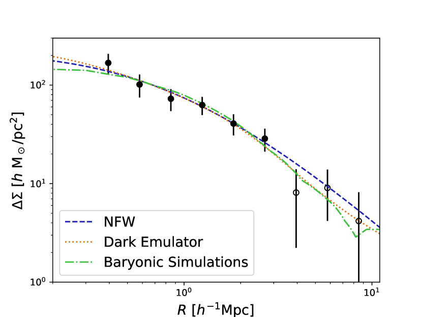
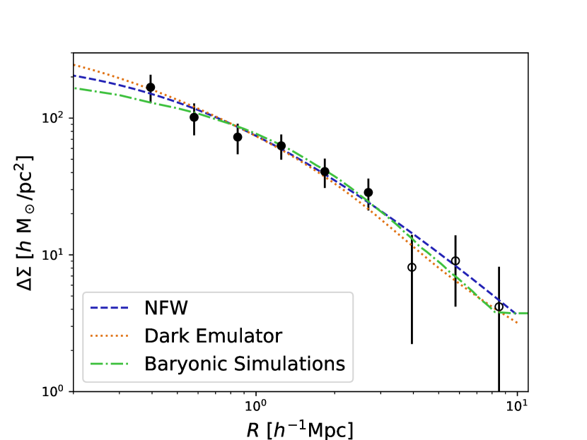
Figure 7.— Left: Single mass-bin fit on the stacked lensing measurement. Right: Stacked model fit on the stacked lensing measurement. The filled circles show data points used for the NFW fit, while both the filled and open circles are used for the Dark Emulator and Baryonic Simulations models.

4.2.2 Stacked Model Method

Here we describe our improved method for estimating the average cluster mass $\langle M_{\mathrm{WL}}\rangle$ from the cluster sample, which we call the Stacked Model method. The essence of the method is to model the stacked lensing profile $\langle\Delta\Sigma\rangle(R)$, accounting for:

• the weak-lensing weighting, which depends on the cluster $z$;

• the cluster (halo) mass function, $dn(z)/dM$;

• the ACTPol cluster selection function, which is known in terms of $M_{SZ}$ and $z$; and

• the mass-mass scaling relationship between $M_{SZ}$ and $M$.

In particular, we define the variables $\mu_{\rm SZ}\equiv{\rm ln}M_{\rm SZ}$ and $\mu\equiv{\rm ln}M$, and we assume

$$\mu_{\rm SZ}=\ B\,\mu+A,$$ (13)

but fix the mass-dependent exponent $B$ to unity, so that we can focus on $A$, which quantifies the constant mass bias between $M_{\rm SZ}$ and the true mass $M$. We qualitatively discuss mass dependence in Section 4.3, but the $S/N$ of our measurement prevents us from providing an interesting constraint on $B$. We consider cluster density profiles from the models described in Section 4.2. To construct a model that can be fit to the data as a function of stacked cluster mass, we compute the stacked lensing profile and stacked mass for different values of $A$, and then interpolate the stacked lensing profile as a function of stacked mass.

The weak-lensing weights are computed for the redshifts $z_{j}$ of the eight clusters as $w_{l}(z_{j},R_{i})=\sum_{s}\tilde{w}_{ls}(R_{i})$, where $s$ includes the subset of source galaxies for the $j$th cluster after the CC cut (Section 3.2). The weak-lensing weights are a smooth function of $z$, and so $w_{l}(z,R_{i})$ is estimated by extrapolation from $w_{l}(z_{j},R_{i})$ for the Dark Emulator and Baryonic Simulations models. The inherent $dn(z)/dM$ from the simulations are self-consistently used for the Dark Emulator and Baryonic Simulations models and for the NFW profile modeling the $dn(z)/dM$ from the Dark Emulator is used. The cluster selection function, $S(M_{\rm SZ},z)$, is computed by averaging the ACTPol survey completeness map, which is defined for a given SZ mass and redshift under our selection criteria SNR${}_{2.4}>5$, over the XMM field where the HSC source galaxies exist (see Section 2.3 for details).

Table 2Parameter constraints from the Single Mass-bin fit and Stacked Model method fit to the stacked lensing data.

	Parameter	NFW	Dark Emulator	Baryonic Simulation
Single Mass-bin
	$M_{\rm WL}$ [1014M⊙]	$4.26^{+0.82}_{-0.71}$	$4.22^{+0.72}_{-0.64}$	$3.67^{+0.86}_{-0.58}$
	$c_{\rm 500c}$	$2.08^{+0.86}_{-0.71}$	N/A	N/A
	$\chi^{2}$/dof	1.3/4	2.5/8	3.4/8
Stacked Model
	$\langle M_{\rm WL}\rangle$ [1014M⊙]	$4.02^{+0.65}_{-0.61}$	$3.89^{+0.61}_{-0.57}$	$3.55^{+0.63}_{-0.48}$
	$1-b$	$0.71^{+0.13}_{-0.12}$	$0.74^{+0.13}_{-0.12}$	$0.80^{+0.16}_{-0.12}$
	$\chi^{2}$/dof	$1.6/5$	$3.0/8$	$3.1/8$

We estimate the conditional probability distribution for $M_{SZ}$ given $M$ assuming it follows a log-normal distribution, such that

$$P(\mu_{\rm SZ}|\mu)=\frac{1}{\sqrt{2\pi}\sigma_{\mu_{\rm SZ}|{\mu}}}\exp{\left[-\frac{\left(\mu_{\rm SZ}-\mu-A\right)^{2}}{2\sigma^{2}_{{\mu_{\rm SZ}|\mu}}}\right]},$$ (14)

where $\sigma_{\mu_{\rm SZ}|{\mu}}$ is the SZ mass-mass scatter which we fix to $\sigma_{\mu_{\rm SZ}|{\mu}}$ = 0.2 for the following reasons. First, the lensing signal does not constrain the scatter well (e.g., Murata et al., 2017). Second, this is the same scatter assumed to correct the Eddington bias for the $M_{\rm SZ}$ values quoted in Hilton et al. (2018) and was used in Battaglia et al. (2016). Thus, using this value for $\sigma_{\mu_{\rm SZ}|{\mu}}$ allows for direct comparison to previous results from ACT.

The Stacked Model lensing signal used for fitting is:

$$\langle\Delta\Sigma\rangle(R_{i}) = \frac{1}{n_{\rm SZ}}\int dzw_{l}(z)\frac{cr^{2}(z)}{H(z)}\int d\mu M\frac{dn}{dM}(z)$$

$$\int d\mu_{\rm SZ}M_{\rm SZ}S(M_{\rm SZ},z)P(\mu_{\rm SZ}|\mu)\Delta\Sigma(R_{i},M,z),$$

Here $r^{2}(z)c/H(z)$ is the comoving volume per unit redshift interval and per unit steradian, $\Delta\Sigma(M,z,R_{i})$ depends on the cluster profile model considered, and $n_{\rm SZ}$ is the expected number density per unit steradian of ACTPol clusters given the weak-lensing weights:

$$n_{\rm SZ} = \int dzw_{l}(z)\frac{cr^{2}(z)}{H(z)}\int d\mu M\frac{dn}{dM}(z)$$ (16)

$$\int d\mu_{\rm SZ}M_{\rm SZ}S(M_{\rm SZ},z)P(\mu_{\rm SZ}|\mu).$$

Finally, we estimate the average mass for the cluster sample as:

$$\langle M_{\rm WL}\rangle = \frac{1}{n_{\rm SZ}}\int dzw_{l}(z)\frac{cr^{2}(z)}{H(z)}\int d\mu M\frac{dn}{dM}(z)$$

$$\int d\mu_{\rm SZ}M_{\rm SZ}S(M_{\rm SZ},z)P(\mu_{\rm SZ}|\mu)M_{\rm WL}(M,z).$$

For the different models of $\Delta\Sigma(R_{i},M,z)$ there are subtle implementation differences that are specific to that model. For the NFW profile, we use the concentration-mass relation derived by Diemer & Kravtsov (2015). Since the mass function in Dark Emulator is defined as a function of $M_{\rm 200m}$, we convert from $M_{\rm 500c}$ to $M_{\rm 200m}$ in the selection function with the concentration-mass relation defined above. For the Dark Emulator profile, we compute the conversion as described in Section 4.2.1.

For the Baryonic Simulations model we calculate the stacked weak-lensing signal as calculated in Battaglia et al. (2016) for a given average sample mass (Eqs. LABEL:eq:delsigstack and LABEL:eq:mfivestack) for each simulated halo surface density profile by the weak-lensing weight, the volume factor (comoving distance squared) associated with each simulation snapshot, the scatter in the scaling relation, and the ACTPol selection function to the simulated halos, described in Hilton et al. (2018).

We summarize the results of fits for $M_{\mathrm{WL}}$ in Table 2 and show the best fit profiles in Figure 7. Similar to the single-mass-bin fit, we restrict the fitting range of the NFW fit to $0.3\>h^{-1}{\rm{Mpc}}<R<3\>h^{-1}{\rm{Mpc}}$, but using the larger radii up to $R\sim 10\>h^{-1}{\rm{Mpc}}$ changes the constraint well within the $1\sigma$ statistical uncertainty. The resulting masses from the Dark Emulator and Baryonic Simulations models are within 10% of each other, which we interpret as the systematic modeling uncertainty for the Stacked Model. This systematic error is still below our $15$% statistical uncertainties on the mass, but with roughly eight more clusters they will become comparable. Looking ahead, if we want to use the full potential statistical power of the HSC survey or other comparable imaging surveys we need to reduce systematic modeling uncertainties.

Comparing the masses from the single-mass-bin fit and the Stacked Model method, we find that the single-mass-bin masses are systematically high by 3 to 7%, depending on the profile model. We interpret this as a systematic bias from the single-mass-bin fitting technique that results from its lack of accounting for the mass and selection functions. Such a bias will become more important as samples of clusters with weak-lensing measurements increase.

4.3. Mass Bias

We present the values for $1-b=\langle M_{\rm SZ}\rangle/\langle M_{\rm WL}\rangle$ in Table 2. We estimate the average SZ mass using the lensing weight to be consistent with the stacking process in lensing measurement; $\langle M_{\rm SZ}\rangle=\sum_{ls}w_{ls}M_{{\rm SZ},l}/\sum_{ls}w_{ls}=2.87^{+0.25}_{-0.20}\ \times 10^{14}\ {\rm M}_{\odot}$. With only eight clusters the precision on the $1-b$ measurement we present in this work has comparable precision to previous measurements which have comparable or larger sample sizes. In Figure 8 we compiled from the literature previous measurements of $1-b$ on ACT and Planck selected clusters from various weak-lensing measurements and include this measurement for comparison. In this work and previous work we directly compare ACT and Planck SZ masses because both ACT and Planck use the same SZ-mass scaling relations and pressure profiles (for more details see Battaglia et al., 2016). However, in the recent ACTPol cluster catalog (Hilton et al., 2018), we found evidence of mass-dependent bias at the 2-$\sigma$ level when we compared the Planck and ACT SZ masses. We are ignoring that fact here since the mass dependence may only be the result of selection effects at the intersection of the Planck and ACT samples. With a much larger sample from ACT in the near future we will be able to address this further.

Previous weak-lensing measurements of Planck clusters von der Linden et al. (2014b) and Hoekstra et al. (2015) show marginal evidence for a mass dependence in $1-b$. Combining these results with the previous ACT clusters result (Battaglia et al., 2016) qualitatively strengthens this evidence. Since Battaglia et al. (2016) was published, several new measurements of $1-b$ were made using Planck SZ clusters. The combination of previous measurements with our new measurement indicates that the observational case for a mass dependence in $1-b$ is weaker (see Figure 8). Simply fitting $1-b$ as a function of mass yields an exponent of $1-b\propto M^{-0.01\pm 0.02}$. Here we have excluded the measurement from LoCuSS (Smith et al., 2016) as their X-ray measurement using spectroscopic-like temperatures (Martino et al., 2014) gives $10\%$ higher X-ray masses in contrast to other measurements and they have a factor of two smaller errors than any other measurements of $1-b$. We caution against any strong conclusions from our simple analysis above, since a proper analysis requires compilation of all the Planck and ACT SZ clusters with weak-lensing measurements, selecting and accounting for multiple weak-lensing measurements of these clusters, and precise Eddington bias corrections that account for the selection functions for each of these surveys convolved with the Planck and ACT selection functions. Comparisons of $1-b$ across different measurements should include sample variance errors, but such errors are typically not included. We calculate the sample variance contribution to $\langle\Delta\Sigma\rangle(R)\rangle$ by randomly sampling halos from the simulations (Battaglia et al., 2010) that satisfy the selection function and find this increases the diagonal of our covariance matrix by 20-30%. Performing similar analyses on all the measurements in Figure 8 will strengthen our conclusions that currently these measurements are consistent and do not show evidence of a mass dependent in $1-b$.

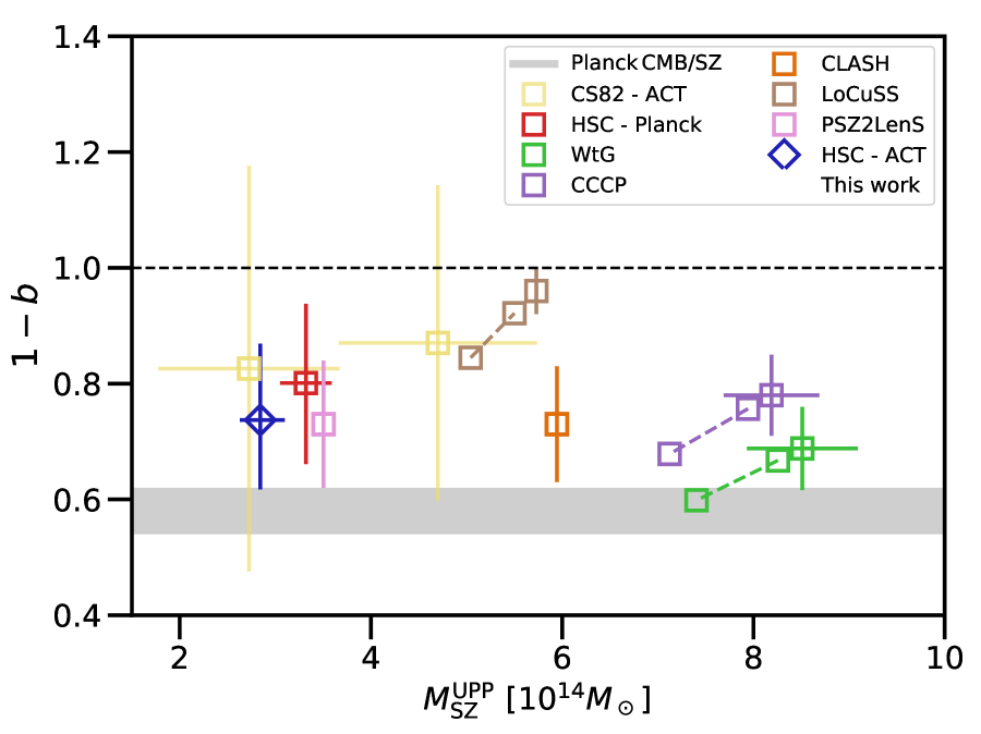
Figure 8.— Current comparison of $1-b$ for clusters with Planck or ACT SZ masses. Here the data points show the ratios of $M^{\rm UPP}_{\rm SZ}$ to $M_{\rm WL}$, and we emphasize that these SZ masses are derived using the profile and X-ray mass scaling relation from Arnaud et al. (2010), which assumes that the intracluster medium is in hydrostatic equilibrium. The grey band indicates the value of $1-b$ required to reconcile the Planck Collaboration et al. (2016d) cluster cosmology results with the Planck Collaboration et al. (2016c) cosmological parameters from the primary CMB fluctuations. The result for this work is shown by the blue diamond from the Dark Emulator fit. Previous $1-b$ measurements by CS82-ACT (Battaglia et al., 2016), LoCuSS (Smith et al., 2016), CLASH (Penna-Lima et al., 2017), PSZ2LenS (Sereno et al., 2017), and HSC-Planck (Medezinski et al., 2018a) are shown in yellow, brown, orange, pink ,and red squares, respectively. The green and purple squares with error bars show the original measurements from WtG (von der Linden et al., 2014b) and CCCP (Hoekstra et al., 2015), respectively, and the same colored squares connected by the dashed lines show the 3-15% range for the Eddington corrected measurements calculated in Battaglia et al. (2016). The weak-lensing mass calibration of ACT SZ masses by HSC is consistent with previous calibrations of ACT and Planck SZ masses, including the LoCuSS measurements after the Eddington bias correction that was applied to von der Linden et al. (2014b) and Hoekstra et al. (2015) is consistently applied to Smith et al. (2016). The error bars here do not include sample variance (see Section 4.3).

5. Discussion and Conclusions

In this work we present weak-lensing observations from the HSC survey of eight ACTPol galaxy clusters selected by their SZ signal. The depth of the HSC survey allows us to make weak-lensing measurements of individual clusters out to $z=1.004$ with $S/N>2$. We stack the weak-lensing measurements of these eight clusters and employ a detailed model for the scaling relation, mass function, and selection function for this sample when we fit for the average weak-lensing mass. The combined signal-to-noise of the stacked weak-lensing measurement is $11.1$. We use three different mass profiles, the NFW profile (analytic), the Dark Emulator (N-body simulation), and the Baryonic Simulations (cosmological hydrodynamic simulations) to infer masses. The average weak-lensing masses inferred for this sample are $\langle M_{\rm WL}\rangle=4.02^{+0.65}_{-0.61}\,10^{14}$M_⊙ , $3.89^{+0.61}_{-0.57}\,10^{14}$M_⊙ and $3.55^{+0.63}_{-0.48}\,10^{14}$M_⊙ for the NFW, Dark Emulator, and Baryonic Simulations Models. We interpret the 10% difference between Dark Emulator and the Baryonic Simulations models as a systematic modeling uncertainty, which is currently lower than our statistical uncertainty. We compare two methods for modeling the stacked signal and demonstrate that using a single mass-bin fit model will introduce systematic biases on the inferred average mass in the range of 3 to 7%.

The weak-lensing measurement of $1-b$ from HSC for ACTPol selected clusters in this work is consistent with previous weak-lensing measurements from the CS82 survey for ACT selected clusters, although the latter has a factor of three times larger errors. Additionally, our measurement of $1-b$ is statistically consistent with previous measurements of Planck SZ clusters and has comparable precision, with only eight clusters in the sample.

Direct comparisons to previous weak-lensing mass calibrations of SPT SZ masses are non-trivial. Unlike Planck and ACT, SPT uses a different filter shape and scaling relation to infer SZ masses (for details see Reichardt et al., 2013; Bleem et al., 2015). In Hilton et al. (2018) we showed that re-calibrated ACT SZ masses from Hasselfield et al. (2013) are in remarkable agreement with the SPT SZ masses in Bleem et al. (2015). However, since there is no overlap in area between the Hilton et al. (2018) and the Bleem et al. (2015) samples, any comparisons would be indirect and require an understanding the sub-sample of selected clusters with weak-lensing measurements. The SPT collaboration is calibrating masses out to and beyond $z=1$ using the Hubble Space Telescope (Schrabback et al., 2016) and SPT’s calibrations are of comparable precision to our measurement (see Dietrich et al., 2017; Stern et al., 2018). Future direct comparisons of $1-b$ between ACT and SPT will be possible as the area surveyed by ACT expands.

Additionally, as the area overlap between the HSC Survey and the ACT experiment increases over the next couple of years we expect the number of clusters to increase roughly proportional to the area. The final area overlap will be of order 1400 deg², which should roughly yield a factor of 40 times more clusters for the same depth CMB maps. This will dramatically reduce the errors on our mass calibration and we can address questions about the mass and redshift dependence of $1-b$.

The underlying goal of calibrating SZ masses is to infer cosmological parameters and we leave such analyses for future work. Here, we will qualitatively estimate how this measurement of $1-b$, when used as a prior for the Planck cosmological cluster analyses, would translate into cosmological parameters. If we take the Dark Emulator fit for $1-b$, which falls between the $1-b$ values of $0.688\pm 0.072$ (von der Linden et al., 2014b) and $0.780\pm 0.092$ (Hoekstra et al., 2015) used in the Planck Collaboration et al. (2016d) cosmological analysis, then the inferred values of cosmological parameters like $\sigma_{8}$ and $\Omega_{m}$ would fall between the respective $\sigma_{8}$ and $\Omega_{m}$ values inferred from the von der Linden et al. (2014b) and Hoekstra et al. (2015) $1-b$ priors. Our $1-b$ measurement is not as precise as the von der Linden et al. (2014b) and Hoekstra et al. (2015) priors so the resulting errors on $\sigma_{8}$ and $\Omega_{\mathrm{m}}$ if applied to the Planck cluster data will also be larger. Thus, we currently cannot address whether there is any actual difference between SZ cluster abundances and CMB primary anisotropy measurements, which is illustrated by differences in $1-b$ (compare the measurements and grey band in Figure 8). We expect that this difference will be revisited after revisions to the primary CMB constraints are made with current and future measurements of the optical depth from polarized primary CMB observations (e.g., Planck Collaboration et al., 2016e), since the $1-b$ inferred here is degenerate with the optical depth for such analyses. We are excited that future HSC and ACT measurements present opportunities to further understand and characterize such differences soon.

Appendix A Details of covariance calculation

A.1. Covariance due to large scale structure

We calculate the covariance due to large scale structure based on Oguri & Takada (2011). For the $n$-th cluster at redshift $z_{n}$ we calculate the covariance due to the projection effect of large scale structure as

$$C^{\rm lss}_{ij,n}=\langle\Sigma_{{\rm cr},ls}^{-1}\rangle^{-2}\int\frac{\ell d\ell}{2\pi}C^{\kappa\kappa}_{\ell}J_{2}\left(\frac{\ell R_{i}}{\chi(z_{n})}\right)J_{2}\left(\frac{\ell R_{j}}{\chi(z_{n})}\right),$$ (A1)

where $J_{2}(x)$ is the second order Bessel function and $\chi(z)$ is the comoving distance at redshift $z$. We approximate the inverse critical surface mass density averaged over source galaxies $\langle\Sigma_{{\rm cr},ls}^{-1}\rangle\sim\Sigma^{-1}_{\rm cr}(z_{n},\langle z_{s}\rangle)$, where $\langle z_{s}\rangle$ is the mean redshift calculated using the photo-$z$ PDF stacked over source galaxies with the weak-lensing weight, i.e.,

$$\langle z_{s}\rangle=\frac{\int dz\ z\ P_{\rm stacked}(z)}{\int dzP_{\rm stacked}(z)},$$ (A2)

where $P_{\rm stacked}(z)=\sum_{s}\tilde{w}_{ls}P(z)/\sum_{s}\tilde{w}_{ls}$ and $s$ runs over source galaxies in all the radial bins after the color-color cut as a function of lens redshift (See Section 3.3 for details). The weak-lensing power spectrum $C^{\kappa\kappa}_{\ell}$ is defined as

$$C^{\kappa\kappa}_{\ell}=\int d\chi\frac{[W^{\kappa}(z)]^{2}}{\chi^{2}}P_{m}^{\rm NL}\left(k=\frac{\ell}{\chi};z\right),$$ (A3)

where $W^{\kappa}(z)$ is the lensing weight function defined by

$$W^{\kappa}(z)=\frac{\rho_{m}(z)\langle\Sigma_{\rm cr}^{-1}\rangle}{(1+z)}.$$ (A4)

Here we again use the same approximation $\langle\Sigma_{\rm cr}^{-1}\rangle\sim\Sigma_{\rm cr}^{-1}(z,\langle z_{s}\rangle)$. The non-linear matter power spectrum $P_{m}^{\rm NL}(k)$ is calculated by CAMB using the Halofit prescription (Smith et al., 2003) with the fitting parameter derived in Takahashi et al. (2012). We then calculate the covariance of the stacked lensing signal as

$$C^{\rm lss}_{ij}=\frac{\sum_{n}\tilde{v}_{n,i}\tilde{v}_{n,j}C^{\rm lss}_{ij,n}}{\sum_{n}\tilde{v}_{n,i}\sum_{l}\tilde{v}_{n,j}},$$ (A5)

where $\tilde{v}_{n,i}$ is the sum of the weak-lensing weight within the $i$-th bin of the $n$-th lens.

A.2. Covariance due to intrinsic variations of projected cluster mass profile

We estimate the covariance that accounts for intrinsic variations of projected cluster mass profile, which includes the scatter in concentration and the triaxiality effect, based on Umetsu et al. (2016). They found that the intrinsic covariance of the lensing convergence $\kappa=\Sigma(R)/\Sigma_{\rm cr}$ can be well approximated by

$$C^{\kappa,{\rm int}}_{ij}=\alpha_{\rm int}^{2}\kappa^{2}\delta_{ij},$$ (A6)

where $\alpha_{\rm int}=0.2$ for $M_{200c}\sim 10^{15}\>h^{-1}\rm M_{\odot}$ clusters. This formalism excludes the external contribution from $C^{\mathrm{lss}}$, which was formally included in $C^{\mathrm{int}}$ covariance by Gruen et al. (2015). We convert Eq. A6 to the covariance of excess surface density $C^{\Delta\Sigma,{\rm int}}_{ij}$ , assuming the NFW profile with concentration-mass relation derived in Diemer & Kravtsov (2015). Therefore, the covariance $C^{\Delta\Sigma,{\rm int}}_{ij}$ depends on cluster mass. Note that, however, covariances with difference cluster mass are actually similar in their shapes and have the same form once they are scaled by $r\rightarrow r/r_{\rm 200m}$. We then approximately calculate the covariance of the stacked lensing signal by

$$C_{ij}^{\rm int}=\frac{C^{\Delta\Sigma,{\rm int}}_{ij}(\langle M\rangle)}{N_{\rm cl}},$$ (A7)

where $\langle M_{\rm WL}\rangle$ (in $M_{\rm 500c}$) is the typical mass of our cluster sample and $N_{\rm cl}$ is the number of clusters. We vary the typical mass within $1.0<\langle M_{\rm WL}\rangle/10^{14}M_{\odot}<7.0$ and see how the $1-b$ constraints are affected. We find the change in $1-b$ is within 1%, and thus use a fixed mass $\langle M_{\rm WL}\rangle=3.5\times 10^{14}M_{\odot}$ for the intrinsic covariance in the main text.

Appendix B Additional Systematic Tests

B.1. Null Tests

B.1.1 B-mode Signal

Since weak lensing is caused by a scalar potential, a 45-degree rotated component from tangential shear, or B-mode, should be statistically consistent with zero. The left panel of Figure 9 shows the stacked B-mode signal around our ACTPol cluster sample. For our fitting range ($0.3\>h^{-1}{\rm{Mpc}}<R<\>h^{-1}{\rm{Mpc}}$), $\chi^{2}/dof=7.05/9$, and thus our B-model signal is consistent with zero.

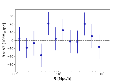
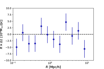
Figure 9.— Left: Stacked lensing B-mode signal around our ACTPol cluster sample. Right: Stacked lensing signal around 200 random points.

B.1.2 Random Signal

If the PSF correction is imperfect, the lensing signal around random points will, statistically, be significantly different from zero. In this case, we need to correct for the imperfect PSF correction by subtracting the random signal from observed lensing signal. We generate random points within the HSC XMM field which follow the cluster redshift distribution based on the cluster mass function with the best fitting parameters of the NFW complete stacked fit (for details, see Section 4.2.2). The right panel of Figure 9 shows the stacked lensing signal around 200 random points. For our fitting range ($0.3\>h^{-1}{\rm{Mpc}}<R<\>h^{-1}{\rm{Mpc}}$), $\chi^{2}/dof=8.75/9$, which shows the random signal is consistent with zero.

B.2. Lensing Signals with Different Photo-$z$ Methods

We use MLZ photo-$z$ estimates for fiducial measurement as described in Section 2.3. In this section we describe the details of other photo-$z$ methods in the HSC SSP catalog and check the consistency between ACTPol cluster lensing signals based on different photo-$z$ methods.

The HSC SSP catalog has photo-$z$ estimates based on the following methods; DEmP, Ephor, Franken-Z, Mizuki, and NNPZ (Tanaka et al., 2018), in addition to MLZ. DEmP is a method designed to minimize major issues of conventional empirical methods, such as how to choose a proper fitting function and biases due to the population of a training data set, by introducing regional polynomial fitting and uniformly weighted training set (Hsieh & Yee, 2014). Ephor is a neural network photo-$z$ code fed with de Vaucouleur flux and exponential flux. Franken-Z is a hybrid approach that combines the data-driven nature of machine learning and statistical rigor from template fitting. Mizuki is a Bayesian template fitting method which allows for simultaneously constraining physical properties of galaxies such as star formation and photo-$z$ (Tanaka, 2015). NNPZ follows the method introduced by Cunha et al. (2009), a nearest neighbor method that finds nearest neighbors around an unknown object in the color/magnitude space from a reference sample and uses the reference redshift histogram as the PDF.

The top panel of Fig. 10 shows lensing signals measured with different photo-$z$s. The fractional residuals between MLZ and other photo-$z$ methods are shown in the bottom panel. When calculating error bars of fractional residuals, we account for the correlation between lensing signals based on different photo-$z$s. To estimate the correlation, we generate 18 realizations of galaxy shape catalogs with randomly rotated shapes. We then measure lensing signals around clusters in the same manner described in Section 3, using different photo-$z$s. Although the signal itself has no tangential shear signal, we can still compute the correlation between lensing signals computed with different photo-$z$s. The inverse-variance weighted average of the fractional residual ranges from $-0.05\pm 0.01$ (Mizuki) to $0.01\pm 0.01$ (Ephor), which is smaller than the expected deviation due to statistical uncertainties of the stacked lensing signal, i.e., $\delta_{\Delta\Sigma}=\left[\sum_{i}\left(\Delta\Sigma(R_{i})/\sigma_{\Delta\Sigma(R_{i})}\right)^{2}\right]^{-1/2}$, where $\sigma_{\Delta\Sigma(R_{i})}$ is the shape noise. Thus we conclude that the relative bias between photo-z methods are within the statistical uncertainties.

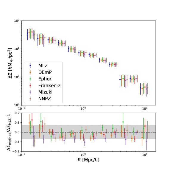
Figure 10.— top: The weak-lensing signals for different photo-$z$ methods. The data points with different photo-$z$ methods are shifted along x-axis for illustrative purposes. bottom: The fractional residuals between MLZ and other methods. Error bars are calculated by taking correlations between different lensing signals into account. The gray region shows the statistical error of our lensing measurement combined across the radial bins. See text for these details.

B.3. Off-centering

If the cluster center used in the lensing measurement (in this case, the BCG position) is offset from the gravitational potential minimum, the lensing signal at inner radii around and below the scale of off-centering is diluted. Previous studies showed that the positions of BCGs are better tracers of potential minima than other optical tracers such as the luminosity-weighted centers (Viola et al., 2015), and than X-ray centers because of the large statistical uncertainties in the X-ray center (George et al., 2012; von der Linden et al., 2014a). We expect this is also the case for our measurement. The ACT beam at 148 GHz is $1.4\arcmin$ and with a 5$\sigma$ SZ detection we expect the astrometric uncertainties to be around $20\arcsec$ at $z\gtrsim 0.5$, which is similar to the typical off-centering except for the cluster J0229.6-0337.

We check the impact of off-centering by comparing the lensing signal calculated with the BCG center to that with the SZ center. The comparison is shown in Figure 11. We do not find a significant difference between these signals, especially at the scales we use when fitting the models ($R>0.3\>h^{-1}{\rm{Mpc}}$), and thus it does not matter which center we use at this regime of signal-to-noise ratio for the stacked signal. Even if the lensing shear profile is affected by the off-centering effect, the enclosed mass should be properly extracted if we use the lensing signals to sufficiently large radii compared to the off-centering distance (see Oguri & Takada, 2011). For our fiducial measurement we use the BCG positions as centers.

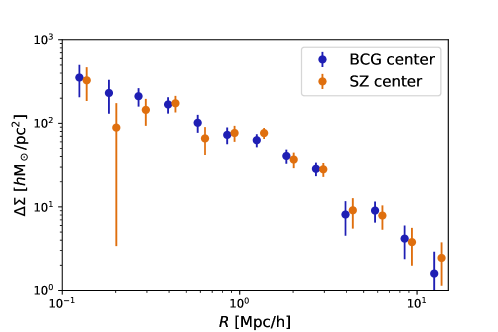
Figure 11.— The stacked weak-lensing signals calculated around different definitions of the cluster centers. The data points with for the SZ centers are shifted along x-axis for illustrative purposes. We do not see a significant difference between whether using the BCG center or the SZ center at the scales we use for model fitting ($R>0.3\>h^{-1}{\rm{Mpc}}$). We use the BCG center for our fiducial measurement.

Appendix C Modeling Stacked Lensing Signal with Sparse Cluster Sampling

In Section 4.2.2, we assumed in our model that the ACTPol clusters sample are representative of the underlying cluster distribution, which is a convolution of the halo mass function and ACTPol selection function. Thus, we integrated the lensing profile along redshift and SZ mass. Here we examine this assumption by replacing the integral in Eqs. LABEL:eq:delsigstack and LABEL:eq:mfivestack with the summation of our cluster sample, i.e.,

$$\langle\Delta\Sigma\rangle(R_{i})=\frac{1}{n_{\rm SZ}}\sum_{j}w_{l}(z_{j})S(M_{{\rm SZ},j},z_{j})\int dM\frac{dn}{dM}(z_{j})P(M_{{\rm SZ},j}|M)\Delta\Sigma(R_{i},M,z_{j}),$$ (C1)

where $n_{\rm SZ}$ becomes

$$n_{\rm SZ}=\sum_{j}w_{l}(z_{j})\int dM\frac{dn}{dM}(z_{j})S(M_{{\rm SZ},j},z_{j})P(M_{{\rm SZ},j}|M),$$ (C2)

and $M_{\rm WL}$ becomes

$$\langle M_{\rm WL}\rangle=\frac{1}{n_{\rm SZ}}\sum_{j}w_{l}(z_{j})S(M_{{\rm SZ},j},z_{j})\int dM\frac{dn}{dM}(z_{j})P(M_{{\rm SZ},j}|M)M_{\rm WL}(M,z_{j}),$$ (C3)

where $M_{{\rm SZ},j}$ is the SZ mass before the Eddington bias correction. We then constrain $1-b$ in the same manner as Section 4.3 for the NFW profile case. We find that the difference in the central value is less than one percent, which is negligible compared to statistical uncertainties. This demonstrates that our analysis method in Section 4.2.2 is unbiased. We note that our test is not a general statement regarding such a bias and should not be applied to other cluster samples.

References

- Aihara et al. (2018a) Aihara, H. et al. 2018a, PASJ, 70, S4
- Aihara et al. (2018b) —. 2018b, PASJ, 70, S8
- Albareti et al. (2017) Albareti, F. D. et al. 2017, ApJS, 233, 25
- Allen et al. (2011) Allen, S. W., Evrard, A. E., & Mantz, A. B. 2011, ARA&A, 49, 409
- Applegate et al. (2014) Applegate, D. E. et al. 2014, MNRAS, 439, 48
- Arnaud et al. (2010) Arnaud, M., Pratt, G. W., Piffaretti, R., Böhringer, H., Croston, J. H., & Pointecouteau, E. 2010, A&A, 517, A92
- Battaglia et al. (2012) Battaglia, N., Bond, J. R., Pfrommer, C., & Sievers, J. L. 2012, ApJ, 758, 74
- Battaglia et al. (2010) Battaglia, N., Bond, J. R., Pfrommer, C., Sievers, J. L., & Sijacki, D. 2010, ApJ, 725, 91
- Battaglia et al. (2016) Battaglia, N. et al. 2016, J. Cosmology Astropart. Phys, 8, 013
- Benson et al. (2013) Benson, B. A. et al. 2013, ApJ, 763, 147
- Bernstein & Jarvis (2002) Bernstein, G. M., & Jarvis, M. 2002, AJ, 123, 583
- Bleem et al. (2015) Bleem, L. E. et al. 2015, ApJS, 216, 27
- Bonnett et al. (2016) Bonnett, C. et al. 2016, Phys. Rev. D, 94, 042005
- Bosch et al. (2018) Bosch, J. et al. 2018, PASJ, 70, S5
- Carbone et al. (2012) Carbone, C., Fedeli, C., Moscardini, L., & Cimatti, A. 2012, J. Cosmology Astropart. Phys, 3, 023
- Carlstrom et al. (2011) Carlstrom, J. E. et al. 2011, PASP, 123, 568
- Coupon et al. (2018) Coupon, J., Czakon, N., Bosch, J., Komiyama, Y., Medezinski, E., Miyazaki, S., & Oguri, M. 2018, PASJ, 70, S7
- Cunha et al. (2009) Cunha, C. E., Lima, M., Oyaizu, H., Frieman, J., & Lin, H. 2009, MNRAS, 396, 2379
- de Haan et al. (2016) de Haan, T. et al. 2016, ApJ, 832, 95
- Diemer (2017) Diemer, B. 2017, ArXiv e-prints
- Diemer & Kravtsov (2015) Diemer, B., & Kravtsov, A. V. 2015, ApJ, 799, 108
- Dietrich et al. (2017) Dietrich, J. P. et al. 2017, ArXiv:1711.05344
- Evrard (1990) Evrard, A. E. 1990, ApJ, 363, 349
- George et al. (2012) George, M. R. et al. 2012, ApJ, 757, 2
- Gruen et al. (2017) Gruen, D. et al. 2017, ArXiv e-prints
- Gruen et al. (2015) Gruen, D., Seitz, S., Becker, M. R., Friedrich, O., & Mana, A. 2015, MNRAS, 449, 4264
- Gruen et al. (2014) Gruen, D. et al. 2014, MNRAS, 442, 1507
- Hasselfield et al. (2013) Hasselfield, M. et al. 2013, J. Cosmology Astropart. Phys, 7, 8
- High et al. (2012) High, F. W. et al. 2012, ApJ, 758, 68
- Hilton et al. (2018) Hilton, M. et al. 2018, ApJS, 235, 20
- Hirata & Seljak (2003) Hirata, C., & Seljak, U. 2003, MNRAS, 343, 459
- Hoekstra et al. (2015) Hoekstra, H., Herbonnet, R., Muzzin, A., Babul, A., Mahdavi, A., Viola, M., & Cacciato, M. 2015, MNRAS, 449, 685
- Hoekstra et al. (2012) Hoekstra, H., Mahdavi, A., Babul, A., & Bildfell, C. 2012, MNRAS, 427, 1298
- Hsieh & Yee (2014) Hsieh, B. C., & Yee, H. K. C. 2014, ApJ, 792, 102
- Ilbert et al. (2009) Ilbert, O. et al. 2009, ApJ, 690, 1236
- Jee et al. (2014) Jee, M. J., Hughes, J. P., Menanteau, F., Sifón, C., Mandelbaum, R., Barrientos, L. F., Infante, L., & Ng, K. Y. 2014, ApJ, 785, 20
- Kaiser (1992) Kaiser, N. 1992, ApJ, 388, 272
- Komiyama et al. (2018) Komiyama, Y. et al. 2018, PASJ, 70, S2
- Lau et al. (2009) Lau, E. T., Kravtsov, A. V., & Nagai, D. 2009, ApJ, 705, 1129
- Louis & Alonso (2017) Louis, T., & Alonso, D. 2017, Phys. Rev. D, 95, 043517
- Louis et al. (2017) Louis, T. et al. 2017, J. Cosmology Astropart. Phys, 6, 031
- Madhavacheril et al. (2017) Madhavacheril, M. S., Battaglia, N., & Miyatake, H. 2017, Phys. Rev. D, 96, 103525
- Mak & Pierpaoli (2013) Mak, D. S. Y., & Pierpaoli, E. 2013, Phys. Rev. D, 87, 103518
- Mandelbaum et al. (2005) Mandelbaum, R. et al. 2005, MNRAS, 361, 1287
- Mandelbaum et al. (2017) —. 2017, ArXiv e-prints
- Mandelbaum et al. (2018) —. 2018, PASJ, 70, S25
- Mandelbaum et al. (2006) Mandelbaum, R., Seljak, U., Cool, R. J., Blanton, M., Hirata, C. M., & Brinkmann, J. 2006, MNRAS, 372, 758
- Mandelbaum et al. (2008) Mandelbaum, R. et al. 2008, MNRAS, 386, 781
- Mandelbaum et al. (2013) Mandelbaum, R., Slosar, A., Baldauf, T., Seljak, U., Hirata, C. M., Nakajima, R., Reyes, R., & Smith, R. E. 2013, MNRAS, 432, 1544
- Mantz et al. (2014) Mantz, A. B., Allen, S. W., Morris, R. G., Rapetti, D. A., Applegate, D. E., Kelly, P. L., von der Linden, A., & Schmidt, R. W. 2014, MNRAS, 440, 2077
- Mantz et al. (2015) Mantz, A. B. et al. 2015, MNRAS, 446, 2205
- Marriage et al. (2011) Marriage, T. A. et al. 2011, ApJ, 737, 61
- Marrone et al. (2012) Marrone, D. P. et al. 2012, ApJ, 754, 119
- Marrone et al. (2009) —. 2009, ApJ, 701, L114
- Martino et al. (2014) Martino, R., Mazzotta, P., Bourdin, H., Smith, G. P., Bartalucci, I., Marrone, D. P., Finoguenov, A., & Okabe, N. 2014, MNRAS, 443, 2342
- McInnes et al. (2009) McInnes, R. N., Menanteau, F., Heavens, A. F., Hughes, J. P., Jimenez, R., Massey, R., Simon, P., & Taylor, A. 2009, MNRAS, 399, L84
- Medezinski et al. (2018a) Medezinski, E. et al. 2018a, PASJ, 70, S28
- Medezinski et al. (2018b) —. 2018b, PASJ
- Miyatake et al. (2013) Miyatake, H. et al. 2013, MNRAS, 429, 3627
- Miyazaki et al. (2018a) Miyazaki, S. et al. 2018a, PASJ, 70, S1
- Miyazaki et al. (2018b) —. 2018b, PASJ, 70, S27
- More S. et al. (in prep.) More S. et al. in prep.
- Motl et al. (2005) Motl, P. M., Hallman, E. J., Burns, J. O., & Norman, M. L. 2005, ApJ, 623, L63
- Murata et al. (2017) Murata, R., Nishimichi, T., Takada, M., Miyatake, H., Shirasaki, M., More, S., Takahashi, R., & Osato, K. 2017, ArXiv e-prints
- Naess et al. (2014) Naess, S. et al. 2014, J. Cosmology Astropart. Phys, 10, 007
- Nagai (2006) Nagai, D. 2006, ApJ, 650, 538
- Nakajima et al. (2012) Nakajima, R., Mandelbaum, R., Seljak, U., Cohn, J. D., Reyes, R., & Cool, R. 2012, MNRAS, 420, 3240
- Navarro et al. (1996) Navarro, J. F., Frenk, C. S., & White, S. D. M. 1996, ApJ, 462, 563
- Navarro et al. (1997) —. 1997, ApJ, 490, 493
- Nelson et al. (2012) Nelson, K., Rudd, D. H., Shaw, L., & Nagai, D. 2012, ApJ, 751, 121
- Nishimichi et al. (in prep.) Nishimichi, T., , , & . in prep.
- Oguri (2014) Oguri, M. 2014, MNRAS, 444, 147
- Oguri et al. (2018) Oguri, M. et al. 2018, PASJ, 70, S20
- Oguri & Takada (2011) Oguri, M., & Takada, M. 2011, Phys. Rev. D, 83, 023008
- Okabe et al. (2010) Okabe, N., Takada, M., Umetsu, K., Futamase, T., & Smith, G. P. 2010, PASJ, 62, 811
- Pacaud et al. (2016) Pacaud, F. et al. 2016, A&A, 592, A2
- Penna-Lima et al. (2017) Penna-Lima, M., Bartlett, J. G., Rozo, E., Melin, J.-B., Merten, J., Evrard, A. E., Postman, M., & Rykoff, E. 2017, A&A, 604, A89
- Planck Collaboration et al. (2016a) Planck Collaboration et al. 2016a, A&A, 594, A1
- Planck Collaboration et al. (2014a) —. 2014a, A&A, 571, A29
- Planck Collaboration et al. (2014b) —. 2014b, A&A, 571, A20
- Planck Collaboration et al. (2016b) —. 2016b, A&A, 594, A27
- Planck Collaboration et al. (2016c) —. 2016c, A&A, 594, A13
- Planck Collaboration et al. (2016d) —. 2016d, A&A, 594, A24
- Planck Collaboration et al. (2016e) —. 2016e, A&A, 596, A107
- Planelles et al. (2017) Planelles, S. et al. 2017, MNRAS, 467, 3827
- Rasia et al. (2012) Rasia, E. et al. 2012, New Journal of Physics, 14, 055018
- Rasia et al. (2004) Rasia, E., Tormen, G., & Moscardini, L. 2004, MNRAS, 351, 237
- Reichardt et al. (2013) Reichardt, C. L. et al. 2013, ApJ, 763, 127
- Reyes et al. (2012) Reyes, R., Mandelbaum, R., Gunn, J. E., Nakajima, R., Seljak, U., & Hirata, C. M. 2012, MNRAS, 425, 2610
- Rowe et al. (2015) Rowe, B. T. P. et al. 2015, Astronomy and Computing, 10, 121
- Rozo et al. (2010) Rozo, E. et al. 2010, ApJ, 708, 645
- Rykoff et al. (2014) Rykoff, E. S. et al. 2014, ApJ, 785, 104
- Schrabback et al. (2016) Schrabback, T. et al. 2016, ArXiv e-prints
- Sehgal et al. (2011) Sehgal, N. et al. 2011, ApJ, 732, 44
- Sembolini et al. (2013) Sembolini, F., Yepes, G., De Petris, M., Gottlöber, S., Lamagna, L., & Comis, B. 2013, MNRAS, 429, 323
- Sereno et al. (2017) Sereno, M., Covone, G., Izzo, L., Ettori, S., Coupon, J., & Lieu, M. 2017, MNRAS, 472, 1946
- Shimon et al. (2011) Shimon, M., Sadeh, S., & Rephaeli, Y. 2011, MNRAS, 412, 1895
- Smith et al. (2016) Smith, G. P. et al. 2016, MNRAS, 456, L74
- Smith et al. (2003) Smith, R. E. et al. 2003, MNRAS, 341, 1311
- Stanek et al. (2010) Stanek, R., Rasia, E., Evrard, A. E., Pearce, F., & Gazzola, L. 2010, ApJ, 715, 1508
- Staniszewski et al. (2009) Staniszewski, Z. et al. 2009, ApJ, 701, 32
- Stern et al. (2018) Stern, C. et al. 2018, ArXiv e-prints
- Sunyaev & Zeldovich (1969) Sunyaev, R. A., & Zeldovich, Y. B. 1969, Nature, 223, 721
- Sunyaev & Zeldovich (1972) —. 1972, Comments on Astrophysics and Space Physics, 4, 173
- Swetz et al. (2011) Swetz, D. S. et al. 2011, ApJS, 194, 41
- Takahashi et al. (2012) Takahashi, R., Sato, M., Nishimichi, T., Taruya, A., & Oguri, M. 2012, ApJ, 761, 152
- Tanaka (2015) Tanaka, M. 2015, ApJ, 801, 20
- Tanaka et al. (2018) Tanaka, M. et al. 2018, PASJ, 70, S9
- Thornton et al. (2016) Thornton, R. J. et al. 2016, ApJS, 227, 21
- Umetsu et al. (2016) Umetsu, K., Zitrin, A., Gruen, D., Merten, J., Donahue, M., & Postman, M. 2016, ApJ, 821, 116
- Vanderlinde et al. (2010) Vanderlinde, K. et al. 2010, ApJ, 722, 1180
- Vikhlinin et al. (2009) Vikhlinin, A. et al. 2009, ApJ, 692, 1060
- Viola et al. (2015) Viola, M. et al. 2015, MNRAS, 452, 3529
- Voit (2005) Voit, G. M. 2005, Reviews of Modern Physics, 77, 207
- von der Linden et al. (2014a) von der Linden, A. et al. 2014a, MNRAS, 439, 2
- von der Linden et al. (2014b) —. 2014b, MNRAS, 443, 1973
- Wang et al. (2005) Wang, S., Haiman, Z., Hu, W., Khoury, J., & May, M. 2005, Physical Review Letters, 95, 011302