Periodic orbits around Kerr Sen black holes

Abstract

Abstract

We investigate periodic orbits and zoom-whirl behaviors around a Kerr Sen black hole with a rational number $q$ in terms of three integers $(z,w,v)$, from which one can immediately read off the number of leaves (or zooms), the ordering of the leaves, and the number of whirls. The characteristic of zoom-whirl periodic orbits is the precession of multi-leaf orbits in the strong-field regime. This feature is analogous to the counterpart in the Kerr space-time. Finally, we analyze the impact of the charge parameter $b$ on the zoom-whirl periodic orbits. Compared to the periodic orbits around the Kerr black hole, it is found that typically lower energies are required for the same orbits in the Kerr Sen black hole.

I Introduction

Periodic orbits have played a crucial role in the treatment of some difficult problems in celestial mechanics, including the motions of planetary satellites, the long term stability of the solar system, and motion in galactic potential. It is fact that the relativistic precession of Mercury s perihelion in the weak field is around a star. In the strong-field, perihelion precession in the equatorial plane of a black hole can result in zoom-whirl orbits for which the precession is so great at closest approach that the particle executes multiple circles before falling out to apastron again. The Laser Interferometer Gravitational-wave Observatory (LIGO) gw1 ; gw2 ; gw3 and VIRGO collaborations reported the observation of gravitational-wave signal corresponding to the inspiral and merger of two black holes is also relevant to this relativistic trajectories. In a series of papers Levin ; Levin1 ; Levin2 ; Levin3 ; Levin4 , Levin et al, proposed a classification of the zoom-whirl structure of the periodic orbits around black hole by using Kerr geodesics sha2 ; Chandra ; wilkins ; Hughes2 ; Barausse ; Ryuichi ; GK ; Celestial ; Mino:2003yg ; Drasco:2004 ; Kostas_Review with a rational number $q$ in terms of three integers $(z,w,v)$

$$q=w+\frac{v}{z}$$ (1)

where $w$ counts the number of whirls, $z$ counts the number of leaves, and $v$ indicates the order in which the leaves are traced out. The rational number $q$ explicitly measures the degree of perihelion precession beyond the ellipse as well as the topology of the orbit. This classification is applied to black hole pairs, they found that zoom-whirl behavior is ubiquitous in comparable mass binary dynamics and entirely quantifiable through the spectrum of rational. This zoom-whirl behavior is also found in the Reissner-Nordstr$\ddot{o}$m black hole Levin3 and spherically symmetric naked singularity gzBabar , Kehagias-Sfetsos black hole shaowen . Furthermore, periodic orbits are generalized from the equatorial taxonomy to fully generic 3D Kerr motion Levin4 .

The Kerr-Sen black hole (KSBH) solution sen is a charged and rotating solution in the low energy limit of heterotic string theory and is also characterized by mass, electric charges, and angular momentum, which are similar to those of the Kerr Newman black hole. Some distinguishable properties and various aspects of particle motion Blaga:2001wt ; Pradhan:2015yea ; Hioki2008zw ; Koga1995bs ; Ghez2012qn ; Furu2004 ; Siahaan2015xna ; Dastan:2016bfy in those space-times have been studied. Based on a topological taxonomy of periodic orbit, in this paper, we will use Levin’s Levin classification scheme to investigate the zoom-whirl behavior and orbital dynamics in the equatorial plane of the KSBH. We will use specific features of the periodic orbits to distinguish KSBH from Kerr black hole.

The paper is organized as follows: In Sec. II, we first derive the relevant geodesic equations of KSBH using the Hamiltonian formulation. In Sec. III, we investigate the innermost bound and stable circular orbits, as well as a qualitative analysis of the effective potential. In Sec.IV, the energy of zoom-whirl periodic orbits in the KSBH is studied. Finally, we end the paper with a summary.

II The time-like geodesic equations in the Kerr Sen black hole

In Ref. sen , Sen obtained a four dimensional solution that describes a rotating and electrically charged massive body in the low energy heterotic string field theory. In the Boyer-Lindquist coordinates, the Kerr-Sen metric can be rewritten as

$$ds^{2}= - \left(1-\frac{2Mr}{\rho^{2}}\right)dt^{2}+\rho^{2}\left(\frac{dr^{2}}{\Delta}+d\theta^{2}\right)-\frac{4Mra\sin^{2}{\theta}}{\rho^{2}}dt{d\phi}$$ (2)

$$+ \left(r(r+b)+a^{2}+\frac{2Mra^{2}\sin^{2}{\theta}}{\rho^{2}}\right)\sin^{2}{\theta}d\phi^{2},$$

where the functions $\Delta$ and $\rho^{2}$ are given by

$$\Delta = r(r+b)-2Mr+a^{2},$$ (3)

$$\rho^{2} = r(r+b)+a^{2}\cos^{2}{\theta}.$$ (4)

Here $M$ is the mass of the black hole, $a$ is the specific angular momentum of the black hole, $b=Q^{2}/M$, $Q$ being the electrical charge of the black hole. In the particular case $b=0$, the above solution is reduced to the Kerr one. The event horizon of the KSBH is located at $r_{H}=\frac{2M-b+\sqrt{(2M-b)^{2}-4a^{2}}}{2}$.

The Hamiltonian of a time-like particle propagating along geodesics in a Kerr Sen black hole can be expressed as

$$H(x_{i},p_{i})=\frac{1}{2}g^{\mu\nu}(x)p_{\mu}p_{\nu}=\frac{\Delta}{2\rho^{2}}p_{r}^{2}+\frac{1}{2\rho^{2}}p_{\theta}^{2}+f(r,\theta,p_{t},p_{\varphi})=-\frac{\mu^{2}}{2},$$ (5)

where $\mu$ is the mass of particle. It is easy to obtain two conserved quantities: the energy $E$ and angular momentum $L$ of the test particles with the following forms

$$E=-p_{t}=-g_{tt}\dot{t}-g_{t\varphi}\dot{\varphi},\;\;\;\;\;\;\;\;\;\;\;\;\;\;L=p_{\varphi}=g_{\varphi\varphi}\dot{\varphi}+g_{\varphi t}\dot{t},$$ (6)

The first integral from the geodesic equations in case of the KSBH are calculated as follows (Blaga:2001wt, ; Pradhan:2015yea, ; Hioki2008zw, ; Koga1995bs, ; Ghez2012qn, ; Furu2004, ; Siahaan2015xna, ; Dastan:2016bfy, ). Following the procedure in Ref Levin , we will convert the first integral equations into Hamiltonian formulation to avoid the numerical difficulties and smoothly plot the time-like zoom-whirl orbits. With the help of Hamilton’s equations

$$\frac{dx^{i}}{d\lambda}=\frac{\partial H}{\partial p_{i}}\,,\;\;\frac{dp_{i}}{d\lambda}=-\frac{\partial H}{\partial x^{i}}\,,$$ (7)

the equations of the time-like particle motion become as,

$$\dot{r} = \frac{\Delta}{\rho^{2}}p_{r},$$ (8)

$$\dot{p}_{r} = -\left(\frac{\Delta}{2\rho^{2}}\right)^{\prime}p_{r}^{2}-\left(\frac{1}{2\rho^{2}}\right)^{\prime}p_{\theta}^{2}+\left(\frac{R+\Delta\Theta}{2\Delta\rho^{2}}\right)^{\prime},$$ (9)

$$\dot{\theta} = \frac{1}{\rho^{2}}p_{\theta},$$ (10)

$$\dot{p}_{\theta} = -\left(\frac{\Delta}{2\rho^{2}}\right)^{\theta}p_{r}^{2}-\left(\frac{1}{2\rho^{2}}\right)^{\theta}p_{\theta}^{2}+\left(\frac{R+\Delta\Theta}{2\Delta\rho^{2}}\right)^{\theta},$$ (11)

$$\dot{t} = \frac{1}{2\Delta\rho^{2}}\frac{\partial(R+\Delta\Theta)}{\partial E},$$ (12)

$$\dot{\varphi} = -\frac{1}{2\Delta\rho^{2}}\frac{\partial(R+\Delta\Theta)}{\partial L},$$ (13)

with

$$R(r) = -\Delta[r(r+b)+Q+(aE-L)^{2}]+[aL-(r(r+b)+a^{2})E]^{2},$$ (14)

$$\Theta(\theta) = Q-\cos^{2}\theta\bigg{(}\frac{L^{2}}{\sin^{2}\theta}+a^{2}(1-E^{2})\bigg{)},$$ (15)

where the superscripts ^′ and $\theta$ denote differentiation with respect to $r$ and $\theta$, respectively. The quantity $Q$ is the generalized Carter constant related to the constant of separation $K$ by $Q=K-(aE-L)^{2}$. In this paper we only deal with the motion of bounded time-like $(\mu=1)$ particles in the equatorial plane, for which motion lies in the 4D hypersurface defined by $\theta=\pi/2$, and on which $Q=0$.

III Bound on angular momentum $L$

As mentioned in Ref Levin , in order to have a sufficiently rich variety of zoom–whirl periodic orbits, the angular momentum $L$ of the particle should satisfies

$$L_{ISCO}<L<L_{IBCO},$$ (16)

where ISCO stands for “Innermost Stable Circular Orbit” and IBCO for “Innermost Bound Circular Orbit”. $L_{ISCO}$ is the lowest value of $L$ for which the potential has a local minimum. For $L<L_{ISCO}$ , all orbits will plunge into the black hole, so $L_{ISCO}$ sets the lower limit on bound orbits. $L_{IBCO}$ marks the first appearance of an unstable circular orbit that is energetically bound. It sets the upper limit only in the sense that we expect to see the most zoom-whirl behavior. From the geodesics, the conditions to determine

,

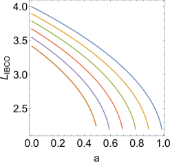
Figure 1: Angular momentum $L_{ISCO}$ and $L_{IBCO}$ vs. $a$ in the Kerr Sen black hole, with Parameter $b=1,0.8,0.6,0.4,0.2,0$ from left to right, here we set $M=1$.

the ISCO are

$$\dot{r}=0,\;\;\;\;\;\ddot{r}=0,\text{and}\;\;\;\;\dddot{r}=0$$ (17)

which yield

$$R(r) = -\Delta[r(r+b)+(aE-L)^{2}]+[aL-(r(r+b)+a^{2})E]^{2}=0,$$ (18)

$$R^{\prime}(r) = -2E(2r+b)(aL-E(a^{2}+r(r+b)))-(2r+b)\Delta-((aE-L)^{2}+r(r+b))\Delta^{\prime}=0,$$

$$R^{\prime\prime}(r) = -4E(aL-E(a^{2}+r(r+b)))+2E^{2}(2r+b)^{2}-2\Delta-(2r+b)\Delta^{\prime}-((aE-L)^{2}+r(r+b))\Delta^{\prime\prime}=0.$$

For the non-rotating black hole, these equations can be solved simultaneously for $E$ and $L$ to give

$$L = \pm\frac{\sqrt{2}Mr(b+r)}{\sqrt{M(b+r)\left(b^{2}+b(3r-2M)+2r(r-3M)\right)}},$$ (19)

$$E = \frac{\sqrt{b+2r}(b-2M+r)}{\sqrt{(b+r)((b+r)(b+2r)-2M(b+3r))}}.$$ (20)

And the radius of the ISCO is given by

$$r_{ISCO}=2M-b+2^{2/3}\sqrt[3]{M^{2}(2M-b)}+\sqrt[3]{2}\sqrt[3]{M(b-2M)^{2}}.$$ (21)

When $b=0$, one will get $r_{ISCO}$ for the Schwarzschild black hole

$$r_{ISCO}/M=6,\quad L_{ISCO}/M\mu=2\sqrt{3},\quad E_{ISCO}=\frac{2\sqrt{2}}{3}.$$ (22)

The radius of the IBCO is given from the condition $E=1$ Bardeen

$$r_{IBCO}=2M-b+\sqrt{2}\sqrt{2M^{2}-bM}.$$ (23)

While when $a\neq 0$, no analytical result is available. Nevertheless, we can obtain a numerical solution. The results are listed in Fig. 1 for prograde orbit. For the prograde ISCO and IBCO , both the angular momentum $L_{ISCO}$ and $L_{IBCO}$ decreases with the black hole spin $a$ and the charge parameter $b$.

For a non-spinning black hole ($a=0$), we can rewrite the radial equation as the expression of effective potential

$$\frac{1}{2}(\dot{r})^{2}+V_{\rm eff}=\frac{E^{2}}{2}\quad,$$ (24)

with

$$V_{\rm eff}=\frac{1}{2}\frac{\Delta~{}\left(L^{2}+r(r+b)\right)}{r^{2}(r+b)^{2}}\quad,$$ (25)

this effective potential $V_{\rm eff}$ is a different function of $r$ for each fixed $L$ and is independent of $E$. The result is a simple visual way to describe the different types of allowed motion as $L$ is varied. However, the effective potential $V_{\rm eff}$ of the spinning Kerr Sen black hole is dependent of $E$. We therefore lose the ability to visualize easily the variation of orbits with energy. A useful pseudo-effective potential Levin3 is constructed through the condition $R(r)=0$ as

$$\left.V_{\rm eff}\right|_{\dot{r}=0}=\frac{E^{2}}{2}\quad,$$ (26)

with

$$E=\frac{\sqrt{r^{2}(b+r)\left(a^{2}+r(b-2M+r)\right)\left(a^{2}(b+2M+r)+(b+r)\left(r(b+r)+L^{2}\right)\right)}+2aLMr}{r\left(a^{2}(b+2M+r)+r(b+r)^{2}\right)}.$$ (27)

.

,

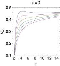
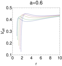
Figure 2: Effective potentials with different the charge parameter $b$ for the corresponding angular momentum $L=L_{av}=\frac{L_{ISCO}+L_{IBCO}}{2}$ in the Kerr Sen black hole: in figure (A), parameter takes the value $b=0,0.2,0.4,0.6,0.8,1$ from top to bottom; in figure (B), parameter takes the value $b=0.69,0.6,0.4,0.2,0$ from left to right. Here we set $M=1$.

Even if the difference between $E$ and the value of $V_{\rm eff}$ no longer gives the value of $\dot{r}^{2}$, this pseudo-effective potential illustrates the change of periodic orbits with energy.

Figure 2 depicts the influence of the charge parameter $b$ to the effective potential. The maximum value of the effective potential decreases with the increasing of the charge parameter $b$. Notice that the corresponding angular momentum $L$ of the effective potential takes the value $L_{av}$ gzBabar (the average value of $L_{ISCO}$ and $L_{IBCO}$)

$$L_{av}=\frac{L_{ISCO}+L_{IBCO}}{2},$$ (28)

this would give an appropriate potential well for any parameter $b$ that captures most of the physics of the bound orbits. In the last section V, the angular momentum $L$ also takes the value $L_{av}$ as we analyze the impact the charge parameter $b$ on the energy of the periodic orbit, in order to have a sufficiently deep potential well that supports a wider variety of orbits .

IV Periodic orbits in Kerr Sen black hole

In this section, we shall study zoom-whirl periodic orbits around the KSBH. We use the taxonomy of orbit of Levin et al. Levin ; Levin1 ; Levin2 ; Levin3 to derive the association between periodic orbits and rational numbers $q$ from the dynamical systems perspective. Any bound orbit may be characterized by two fundamental frequencies–the libration in the radial coordinate, $\omega_{r}$ , and the rotation in the angular coordinate, $\omega_{\varphi}$. Zoom-whirl periodic orbit corresponds to trajectories where the ratio of these two frequencies is a rational number $q$ in terms of three integers $(z,w,v)$,

$$q=w+\frac{v}{z}\equiv\frac{\omega_{\varphi}}{\omega_{r}}-1=\frac{\Delta\varphi}{2\pi}-1,$$ (29)

where $\Delta\varphi=\int^{T_{r}}(d\varphi/dt)dt$ is the equatorial angle accumulated in one radial cycle from apastron to apastron. By this definition, we see that $q$ is the amount an orbit precesses beyond the closed ellipse. These three quantities $z,w,v$ have a geometric interpretation in terms of the structure of the trajectory, where $z$ is the ‘zoom’ number, $w$ is the number of ‘whirls’, and $v$ is the number of vertices formed by joining the successive apastra of the orbits Levin . Thus the trajectory will close and the particle returns to its initial state within a finite (affine) time, thus executing its prior trajectory repeatedly.

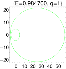
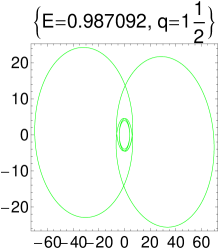
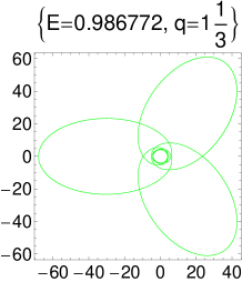
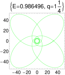
Figure 3: Zoom-whirl periodic orbits with $q=w+\frac{v}{z}=1+\frac{1}{z}$, (z = 1, 2, 3, 4) for $a=0$, $b=0.2$, $L=3.8$, here we set $M=1$.

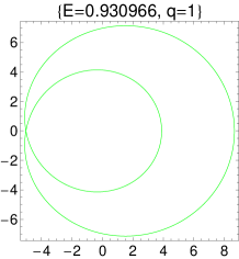
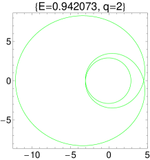
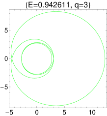
Figure 4: Zoom-whirl periodic orbits with $q=w+\frac{v}{z}=w+\frac{0}{1}$, $(w=1,2,3)$ for $a=0.6$, $b=0.1$, $L=2.9$, here we set $M=1$.

,,

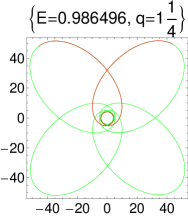
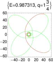
Figure 5: Zoom-whirl periodic orbits with $q=w+\frac{v}{z}=1+\frac{v}{4}$, $(v=1,3)$ for $a=0.$, $b=0.2$, $L=3.8$, here we set $M=1$.

Using the geodesic equations of the KSBH, we get the expression of the rational number $q$,

$$q = \frac{2}{2\pi}\int_{r_{p}}^{r_{a}}\frac{\dot{\varphi}}{\dot{r}}dr-1\quad$$

$$= \frac{1}{\pi}\int_{r_{p}}^{r_{a}}\left(\frac{-\left(aE-L\right)+\frac{a}{\Delta}((r(r+b)+a^{2})E-aL_{z})}{\sqrt{R}}\right)dr-1,\quad$$

where $r_{p}$ and $r_{a}$ is the periastron and apastron of the zoom-whirl orbit, respectively. In the equatorial plane, one of the roots is always $0$ and $R$ can be written as

$$R(r)=(E^{2}-1)r(r-r_{0})(r-r_{p})(r-r_{a}).$$ (31)

Now the rational number $q$ is a function of $q(a,b,E,L,r_{0},r_{p},r_{a})$. To have $q$ as a function of $(a,b,E,L)$ only, we have to find $r_{0},r_{p},r_{a}$ as functions of $(a,b,E,L)$. Thus we expand the polynomial $R(r)=(E^{2}-1)r(r-r_{0})(r-r_{p})(r-r_{a})$ and equate to the definition of $R(r)$ in Eq. (14), matching up coefficients in powers of $r$ and finding a system of equations for $r_{0},r_{p},r_{a}$. Since $r=0$ is always a root, this is equivalent to a 3rd order equation in $r$ and cubic equation have a generic solution. The cubic equation is given as

$$Ar^{3}+Br^{2}+Cr+D=0,\\$$

with

$$A =(E^{2}-1),~{}~{}~{}~{}~{}~{}~{}~{}~{}~{}~{}~{}~{}~{}~{}~{}~{}~{}~{}~{}~{}~{}~{}~{}~{}~{}~{}B=2-2b+2E^{2}b,$$

$$C =Aa^{2}-L^{2}+2b-b^{2}+E^{2}b^{2},~{}~{}D=2(L-aE)^{2}-a^{2}bA-L_{z}^{2}b.$$ (32)

The nonzero roots in ascending order are

$$r_{0} =-\frac{B}{3A}-\frac{2^{1/3}(-B^{2}+3AC)}{3A}(F+\sqrt{G})^{-1/3}+\frac{1}{3A2^{1/3}}(F+\sqrt{G})^{1/3},$$

$$r_{p} =-\frac{B}{3A}+\frac{(1-i\sqrt{3})(-B^{2}+3AC)}{3A2^{2/3}}(F+\sqrt{G})^{-1/3}-\frac{1+i\sqrt{3}}{6A2^{1/3}}(F+\sqrt{G})^{1/3},$$

$$r_{a} =-\frac{B}{3A}+\frac{(1+i\sqrt{3})(-B^{2}+3AC)}{3A2^{2/3}}(F+\sqrt{G})^{-1/3}-\frac{1-i\sqrt{3}}{6A2^{1/3}}(F+\sqrt{G})^{1/3},$$ (33)

where

$$F =-2B^{3}+9ABC-27A^{2}D,$$

$$G ={F^{2}-4(B^{2}-3AC)^{3}}.\quad\quad$$ (34)

We now have established a simple relationship between rational number $q$ and the quantities $a$, $b$, $L$ and $E$, by inputting the value of $z,w$ and $v$ for a given $a$, $b$ and $L$ to locate the $E$, apastron $r_{a}$ and perihelion $r_{p}$ of the corresponding periodic orbit.

In Figure 3, we depict zoom-whirl periodic orbits with various $z$ values. When $z$ increases from $1$ to $4$, the leave of the zoom-whirl periodic orbits varying from one leaf to four leaves. So “$z$” is visualized as the number of leaves, or “zoom” in the particle orbit. Figure 4 shows orbits with various $w$ values, every object travels at least a full from $4\pi$ around to $8\pi$ the central black hole as $w$ increases from $1$ to $3$. It means that the number of extra turns around the center of the geometry gives us the value of $w$. Figure 5 illustrates zoom-whirl orbits with various $v$ values, red line shows that the zoom-whirl orbits with $v=1$ and $v=3$ move along the different trajectory; the energy of the zoom-whirl orbit with $v=3$ is higher than the zoom-whirl orbit with $v=1$.

Finally, we must address the degeneracy that arises when the quotient $v/z$ is a reducible fraction. Thus we require that $v/z$ is an irreducible fraction. As $q$ have approximate values, the zoom-whirl orbit is precessions. For instance, $v/z=42/125\approx 1/3$, the orbit with $q=167/125$ is the precessions of the orbit with $q=4/3$. Figure 6 shows several pairs of the precession orbits. All orbits with $z=1,2,3,4$ are drawn. Between each of these low leaf orbits, randomly selected high zoom orbits are shown as well. The high zoom orbits ( the second and fourth rows of Fig. 6) look like precessions of the low zoom orbits ( the first and third rows of Fig. 6)Levin . That is to say, any aperiodic orbit will be arbitrarily well approximated by a nearby periodic orbit.

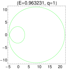
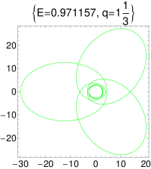
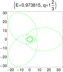
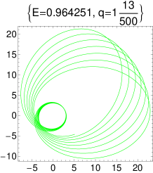
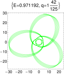
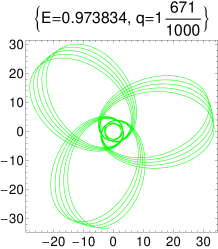
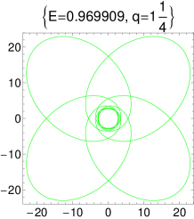
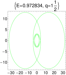
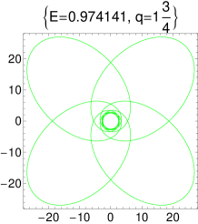
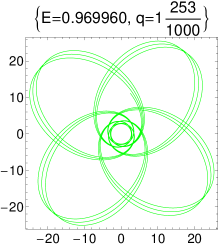
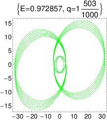
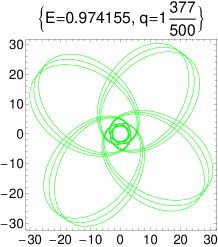
Figure 6: A series of periodic orbits with $a=0.6$, $b=0.18$, $L=3$, $M=1$. Notice that the high $z$ orbits look like precessions of the energetically closest low $z$.

,,

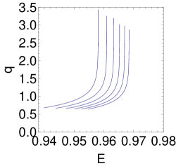
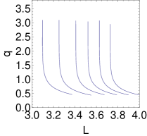
Figure 7: The variation of $q$ as a function of energy $E$ and angular momentum $L$ for different values of $b$ in non-rotating KSBH: decreasing from left to right the values are $1,0.8,0.6,0.4,0.2$, and $0$. In figure (a), for each $b$ depicted above, the corresponding angular momentum is $L_{\mathrm{av}}=(L_{IBCO}+L_{ISCO})/2$ . In figure (b), energy is kept fixed when $(z,w,v)=(2,1,1)$.

,,

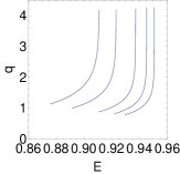
Figure 8: The variation of $q$ as a function of energy $E$ and angular momentum $L$ for different values of the charge parameter $b$ in Kerr sen black hole with the fixed rotating parameter $a=0.6$ : decreasing from left to right the values are 0.69, 0.6, 0.4, 0.2, and 0. In figure (a), for each $b$ depicted above, the corresponding angular momentum is $L_{\mathrm{av}}=(L_{IBCO}+L_{ISCO})/2$ . In figure (b), energy is kept fixed when $(z,w,v)=(2,1,1)$.

$\nu$	$L_{\mathrm{av}}$	$E_{(1,1,0)}$	$E_{(2,1,1)}$	$E_{(3,1,1)}$	$E_{(4,1,1)}$
0.	3.732205	0.965425	0.968026	0.967644	0.967334
0.2	3.63135	0.963682	0.966493	0.966076	0.965739
0.4	3.52488	0.961665	0.964732	0.964272	0.963902
0.6	3.41151	0.959287	0.962679	0.962163	0.961752
0.8	3.28968	0.956420	0.960235	0.959646	0.959179
1	3.15715	0.952848	0.957235	0.956546	0.956004

Table 1: The energy values of $(z=1,2,3,4,w=1,v=1)$ orbits around the non-rotating(a=0) Kerr sen black hole for various $b$ are presented with their corresponding angular momentum, $L_{\mathrm{av}}=(L_{IBCO}+L_{ISCO})/2$.

$\nu$	$L_{\mathrm{av}}$	$E_{(1,1,0)}$	$E_{(2,1,1)}$	$E_{(3,1,1)}$	$E_{(4,1,1)}$
0.	3.01045	0.940589	0.948703	0.947290	0.946238
0.2	2.84151	0.932128	0.942378	0.940520	0.939166
0.4	2.63995	0.918633	0.932594	0.929914	0.928020
0.6	2.37410		0.913234	0.908632	0.905548
0.69	2.20509		0.893783	0.887242	0.883039

Table 2: The energy values of $(z=1,2,3,4,w=1,v=1)$ orbits around the rotating(a=0.6) Kerr sen black hole for various $b$ are presented with their corresponding angular momentum, $L_{\mathrm{av}}=(L_{IBCO}+L_{ISCO})/2$.

V Energy of generic orbits

Zoom-whirl periodic orbits give us a way to visually inspect orbits in different space-time to understand whether we can distinguish the KSBH from the Kerr black hole. So now we analyze the impact of the charge parameter $b$ on the zoom-whirl periodic orbits. Transitions in the periodic orbits can be observed when the energy $E$ and angular momentum $L$ changes, which emanate in the form of gravitational waves. Rational number $q$, as a function of $q(a,b,E,L)$, contains the information on transitions in the periodic orbits during the inspiral stage. Figures 7 and 8 indicate that rational number $q$ monotonically increases with $E$ and decreases with $L$ when the charge parameter $b$ takes the values $1,0.8,0.6,0.4,0.2$, and $0$ in both the rotating and not-rotating KSBHs. Taking $(z=1,2,3,4,w=1,v=1)$ and $L_{\mathrm{av}}=(L_{IBCO}+L_{ISCO})/2$, we list the corresponding energy for each periodic orbit in Tables 1 and 2. It is shown that the corresponding energy $E$ for each periodic orbit decreases with the charge parameter $b$. It implies that the particles in the KSBH with angular momentum $L_{\mathrm{av}}$ in a sufficiently deep potential well possess a richer variety of bound periodic orbits and a wider range of energy $E$ than their Kerr black hole counterparts.

VI summary

In this paper, we have studied periodic orbits in the equatorial plane around the KSBH with a rational number $q$ in terms of three integers $(z,w,v)$ under the taxonomy of orbit of Levin et al. Levin ; Levin1 ; Levin2 ; Levin3 ; Levin4 . By using the Hamiltonian formulation, the geodesic motion of a time-like particle in the KSBH was analyzed, and the bound on the innermost bound and stable circular orbits were also calculated. We found that the angular momentum $L_{ISCO}$ and $L_{IBCO}$ decreases with the black hole spin $a$ and the charge parameter $b$. We showed that all eccentric periodic orbits around the KSBH show zoom whirl behavior of some kind for the angular momentum of the time-like particles in the region $L_{ISCO}<L<L_{IBCO}$. The characteristic of the zoom-whirl periodic orbits is a spectrum of multi-leaf clovers structure, what’s more, aperiodic orbits will look like precessions of low-leaf clovers in the strong-field regime. This feature is qualitatively similar to those in the Kerr space-time. Finally, we analyzed the impact of the charge parameter $b$ on the zoom-whirl periodic orbits to distinguish the KSBH from the Kerr black. We found that periodic orbits around the KSBH occur at lower energies than their Kerr black hole counterparts. These results may provide us a possible observational signature by testing these periodic orbits around the central source to distinguish the KSBH from the Kerr black hole.

VII Acknowledgments

Changqing’s work was supported by the National Natural Science Foundation of China under Grant Nos.11447168. Chikun’s work was supported by the National Natural Science Foundation of China under Grant Nos11247013; Hunan Provincial Natural Science Foundation of China under Grant Nos. 12JJ4007 and 2015JJ2085.

References

- (1)
- (2) B. Abbott et al. , Phys. Rev. Lett. 116, 241103 (2016).
- (3) B. Abbott et al. , Phys. Rev. Lett. 118, 221101 (2017).
- (4) B. Abbott et al. , Phys. Rev. Lett. 119, 141101 (2017).
- (5) J. Levin and G. Perez-Giz, Phys. Rev. D 77, 103005 (2008).
- (6) J. Levin and B. Grossman, Phys. Rev. D 79, 043016 (2009).
- (7) J. Levin, Class. Quant. Grav 26, 235010 (2009).
- (8) V. Misra and J. Levin, Phys. Rev. D 82, 083001 (2010).
- (9) R. Grossman,J. Levin and G. Perez-Giz, Phys. Rev. D 85, 023012 (2012)
- (10) J. M. Bardeen, in Black Holes (Les Astres Occlus), edited by C. DeWitt and B. DeWitt (Gordon and Breach, New York, 1973), p. 215-239.
- (11) S.Chandrasekhar Mathematical theory of black holes (Oxford: Oxford University Press,1983)
- (12) D.C. Wilkins Phys. Rev. D 5, 814 (1972)
- (13) S. A. Hughes Phys. Rev. D 63, 064016 (2001)
- (14) E.Barausse ,S. A. Hughes and L. Rezzolla, Phys. Rev. D 76, 044007 (2007)
- (15) R. Fujita, W. Hikida, Class. Quantum Grav. 26, 135002 (2009)
- (16) K. Glampedakis and D. Kennefick Phys. Rev. D 66, 044002 (2002)
- (17) W.Schmidt, Class. Quantum Grav. 19, 2743 (2002)
- (18) Y. Mino, Phys. Rev .D 67, 084027 (2003)
- (19) S.Drasco and S. A. Hughes Phys. Rev. D 69, 044015 (2004)
- (20) K.Glampedakis 2005 Class. Quantum Grav. 22, S605 (2005).
- (21) G. Z. Babar, A. Z. Babar and Y. Lim, Phys. Rev .D 96, 084052 (2017)
- (22) S. Wei, J. Yang and Y. Liu, Phys. Rev .D 99, 104016 (2019)
- (23) A. Sen, Phys. Rev. Lett. 69, 1006 (1992).
- (24) P. A.Blaga and C. Blaga Class. Quant. Grav. 18, 3893 (2001).
- (25) P.Pradhan, Eur. Phys. J. C 76, no.3 131 (2016).
- (26) K. Hioki and U.Miyamoto, Phys. Rev. D 78, 044007 (2008)
- (27) J. Koga and K. Maeda, Phys. Rev. D 52, 7066 (1995).
- (28) A. M. Ghezelbash and H. M. Siahaan,Class. Quant. Grav. 30, 135005 (2013).
- (29) H.Furuhashi and Y. Nambu, Prog. Theor. Phys. 112, 983 (2004).
- (30) H. M. Siahaan, Int. J. Mod. Phys.D 24, 1550102 (2015).
- (31) S.Dastan, R.Saffari and S. Soroushfar , arXiv:gr-qc 1610.09477.
- (32) J. Bardeen, W. H. Press and S. Teukolsky, Astrophys. J, 178, 347 (1972).