Efimov Physics in Quenched Unitary Bose Gases

Abstract

We study the impact of three-body physics in quenched unitary Bose gases, focusing on the role of the Efimov effect. Using a local density model, we solve the three-body problem and determine three-body decay rates at unitary, finding density-dependent, log-periodic Efimov oscillations, violating the expected continuous scale-invariance in the system. We find that the breakdown of continuous scale-invariance, due to Efimov physics, manifests also in the earliest stages of evolution after the interaction quench to unitarity, where we find the growth of a substantial population of Efimov states for densities in which the interparticle distance is comparable to the size of an Efimov state. This agrees with the early-time dynamical growth of three-body correlations at unitarity [Colussi et al., Phys. Rev. Lett. 120, 100401 (2018)]. By varying the sweep rate away from unitarity, we also find a departure from the usual Landau-Zener analysis for state transfer when the system is allowed to evolve at unitarity and develop correlations.

Over the past few years, the study of strongly interacting Bose gases has greatly intensified due to the experimental advances with ultracold atoms fletcher2013PRL ; rem2013PRL ; makotyn2014NTP ; eismann2016PRX ; chevy2016JPB ; fletcher2017Sci ; laurent2017PRL ; klauss2017PRL ; eigen2017PRL ; fletcher2018ARX , unraveling universal properties and other intriguing phenomena ho2004PRL ; diederix2011PRA ; weiran2012PRL ; jiang2014PRA ; laurent2014PRL ; yin2013PRA ; sykes2014PRA ; rossi2014PRA ; smith2014PRL ; braaten2011PRL ; werner2012PRA ; piatecki2014NTC ; kira2015NTC ; barth2015PRA ; corson2015PRA ; tommaso2016PRL ; yin2016PRA ; jiang2016PRA ; ding2017PRA ; colussi2018PRL ; sze2018PRA ; blume2018PRA . Although ultracold quantum gases have extremely low densities, $n$, the unique ability to control the strength of the interatomic interactions —characterized by the $s$-wave scattering length, $a$— via Feshbach resonances chin2010RMP allows one to probe the unitary regime ($n|a|^{3}\gg 1$), where the probability for collisions can reach unity value and the system becomes non-perturbative. In contrast to their fermionic counterparts giorgini2008RMP ; holland2001PRL ; kokkelmans2002PRA , unitary Bose gases are susceptible to fast atomic losses dincao2004PRL that can prevent the system from reaching equilibrium. In Ref. makotyn2014NTP , a quench of the interactions from weak to strong allowed for the study of the dynamical evolution and equilibration of the unitary Bose gas, thanks to the surprisingly slow three-body decay rates sykes2014PRA . By making the unitary regime accessible, this new quenched scenario opened up intriguing ways to study quantum few- and many-body non-equilibrium dynamics in a controlled manner polkovnikov2011RMP ; rigol2008NT ; dziarmaga2010AP ; gring2012Sci ; cazalilla2012PRE ; zurec2005PRL .

Our understanding of how correlations evolve and subsequently equilibrate in quenched unitary Bose gases is evolving as recent experiments probe physics in this regime fletcher2013PRL ; rem2013PRL ; makotyn2014NTP ; eismann2016PRX ; chevy2016JPB ; fletcher2017Sci ; klauss2017PRL ; eigen2017PRL ; fletcher2018ARX . Most of the current theoretical approaches, however, are based on the two-body physics alone, leaving aside the three-body Efimov physics efimov1979SJNP ; efimov1973NPA ; braaten2006PRep ; wang2013Adv ; naidon2017RPP ; dincao2018JPB ; greene2017RMP . In particular, at unitarity ($|a|=\infty$), although no weakly bound two-body state exists, an infinity of Efimov states form. Critical aspects such as the three-body loss rates and dynamical formation of Efimov state populations remain unexplored within the non-equilibrium scenario of quenched unitary Bose gases.

In this Letter, we explore various aspects related to the three-body physics in quenched unitary Bose gases. We solve the three-body problem using a simple local model, incorporating density effects through a local harmonic trap and describing qualitatively Efimov physics embedded in a larger many-body system. Within this model, we determine loss rates at unitarity that display density-dependent, log-periodic oscillations due to Efimov physics. We also analyze the dynamical formation of Efimov states when the quenched system is held at unitarity and then swept away to weak interactions. This scheme was recently implemented for an ultracold gas of ⁸⁵Rb atoms klauss2017PRL , where a population of Efimov states in a gas phase was observed for the first time. Our present study analyzes such dynamical effects and demonstrates that for densities where the interparticle distance is comparable to the size of an Efimov state, their population is enhanced. This is consistent with a recent theoretical study on the early-time dynamical growth of three-body correlations colussi2018PRL , providing additional evidence for the early-time violation of the universality hypothesis for the quenched unitary Bose gases ho2004PRL . By studying the dependence of the populations on the sweep time, we find a departure from the usual Landau-Zener model of the state formation as the system evolves at unitarity and develops correlations.

Within the adiabatic hyperspherical representation suno2002PRA ; dincao2005PRA ; wang2011PRA ; wang2012PRL , the total three-body wave function for a given state $\beta$ is decomposed as

$$\psi_{\beta}(R,\Omega)=\sum_{\nu}F_{\beta\nu}(R)\Phi_{\nu}(R;\Omega),$$ (1)

where $\Omega$ collectively represents the set of all hyperangles, describing the internal motion and overall rotations of the system, and the hyperradius, $R$, gives the overall system size. The channel functions $\Phi_{\nu}$ are eigenstates of the hyperangular part of the Hamiltonian (including all interatomic interactions) whose eigenvalues are the hyperspherical potentials, obtained for fixed values of $R$. Bound and scattering properties of the system are determined by solving the three-body hyperradial Schrödinger equation,

$$\left[-\frac{\hbar^{2}}{2\mu}\frac{d^{2}}{dR^{2}}+W_{\nu}(R)\right]F_{\nu}(R)$$

$$~{}~{}~{}~{}~{}~{}+\sum_{\nu\neq\nu^{\prime}}W_{\nu\nu^{\prime}}(R)F_{\nu^{\prime}}(R)=EF_{\nu}(R),$$ (2)

where $\mu=m/\sqrt{3}$ is the three-body reduced mass and $\nu$ an index that includes all quantum numbers necessary to characterize each channel. The hyperradial motion is then described by Eq. (2) and is governed by the effective three-body potentials $W_{\nu}$ and nonadiabatic couplings $W_{\nu\nu^{\prime}}$. In our model, we assume atoms interact via a Lennard-Jones potential, $v(r)=-C_{6}/r^{6}(1-\lambda^{6}/r^{6})$, where $C_{6}$ is the dispersion coefficient chin2010RMP , and $\lambda$ is a parameter adjusted to give the desired value of $a$, tuned such that only a single $s$-wave dimer can exist SupMat . The correct three-body parameter wang2012PRL ; naidon2014PRA ; naidon2014PRL , found in terms of the van der Waals length $r_{\rm vdW}=(mC_{6}/\hbar^{2})^{1/4}/2$ chin2010RMP , is naturally built into this potential model, providing a more realistic description of the problem.

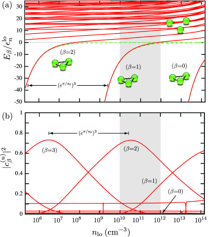
Figure 1: (a) Energies, $E_{\beta}$ [in units of $\epsilon_{n}^{\rm lo}=\hbar^{2}(6\pi^{2}{n_{\rm lo}})^{2/3}/2m$], of three-identical bosons at $|a|=\infty$ as a function of the local density, $n_{\rm lo}$. The dashed green lines represent the free space Efimov state energies. (b) The corresponding population of three-body states, $|c_{\beta}|^{2}$, for quenching to unitarity. The shaded region marks the range of densities where we have studied the dynamical formation of Efimov states.

In order to qualitatively incorporate density effects in our calculations, we introduce a local harmonic confinement whose properties are determined from the average atomic density, $\langle n\rangle$ goral2004JPB ; borca2003NJP ; stecher2007PRL ; sykes2014PRA . This allows us to connect local few-body properties to density-derived scales of the gas, including the system’s energy, $\epsilon_{n}=\hbar^{2}(6\pi^{2}\langle{n}\rangle)^{2/3}/2m$, length scales, $k_{n}^{-1}=\hbar/(2m\epsilon_{n})^{1/2}$, and time scales, $t_{n}=\hbar/\epsilon_{n}$. In the hyperspherical representation, local harmonic confinement is achieved by adding a hyperradial harmonic potential werner2006PRL ; blume2012RPP ,

$$V_{\rm ho}(R)=\frac{\mu\>\omega_{\rm ho}^{2}}{2}R^{2},$$ (3)

to the effective potentials $W_{\nu}$ in Eq. (2). Here, $\omega_{\rm ho}=\hbar/ma_{\rm ho}^{2}$ is the trapping frequency and $a_{\rm ho}$ is the oscillator length. A priori, there is no unique way to relate the harmonic confinement in our model to the atomic density. Nevertheless, as shown in Refs. goral2004JPB ; borca2003NJP ; stecher2007PRL ; sykes2014PRA ; colussi2018PRL ; corson2015PRA , calibrating the local trapping potential [Eq. (3)] to match the few-body density with the interparticle spacing ($\sim\langle n\rangle^{-1/3}$) qualitatively describes the larger many-body system for time scales shorter than $t_{\rm ho}=1/\omega_{\rm ho}$. Here, we relate the local atomic density, $n_{\rm lo}$, and local trapping potential by

$$n_{\rm lo} =\bigg{[}\frac{4\pi}{3}\big{\langle}\psi_{i}\big{|}R^{3}\big{|}\psi_{i}\big{\rangle}\bigg{]}^{-1}\propto\frac{1}{a_{\rm ho}^{3}},$$ (4)

where $\psi_{i}$ is the three-body wave function of the lowest trap state in the regime of weak interactions. The results of this Letter were obtained using $\psi_{i}$ relevant for the ⁸⁵Rb experiment klauss2017PRL , in which the pre-quench, initial state corresponds to $a\approx 150a_{0}$.

In free space, and in the absence of a background gas, the energies of Efimov states at unitarity, $E_{\rm 3b}$, accumulate near the free-atom threshold ($E=0$), and their corresponding sizes, $R_{\rm 3b}$, increase according to the characteristic log-periodic geometric scaling braaten2006PRep :

$$E_{\rm 3b}^{(j)}=-\frac{\hbar^{2}\kappa_{*}^{2}/m}{(e^{\pi/s_{0}})^{2j}}\mbox{~{}~{}and~{}~{}}R_{\rm 3b}^{(j)}=\frac{(1+s_{0}^{2})^{\frac{1}{2}}}{({3}/{2})^{\frac{1}{2}}\kappa_{*}}(e^{\pi/s_{0}})^{j},$$ (5)

where $j$=0, 1, …, labels each Efimov state according to their excitation, $\kappa_{*}\approx 0.226/r_{\rm vdW}$ is the three-body parameter  wang2012PRL , and $e^{\pi/s_{0}}\approx 22.7$ is Efimov’s geometric factor for identical bosons. In the unitary Bose gas, however, one expects that only Efimov states with binding energies larger than $\epsilon_{n}$, and sizes smaller than $k_{n}^{-1}$ are insensitive to the background gas and can exist in their free-space form. Otherwise, Efimov states should be sensitive to the background gas, represented here by a local trapping potential. To illustrate this sensitivity within our model, the energy levels, $E_{\beta}$, of three-identical bosons at $|a|=\infty$ as a function of $n_{\rm lo}$ are shown in Fig. 1(a), displaying geometric scaling as $n_{\rm lo}$ is increased by a factor $(e^{\pi/s_{0}})^{3}\approx 1.17\times 10^{4}$. Within our model, as the energy of a Efimov state approaches $\epsilon_{n}^{\rm lo}$ its value is shifted away from its value in free-space [green dashed lines in Fig. 1(a)]. In order to describe loss processes within our model, we have also provided a finite width (lifetime) for the states, $\Gamma_{\beta}$ ($\tau_{\beta}=\hbar/\Gamma_{\beta}$), adjusted to reproduce the known behavior of the Efimov physics in ⁸⁵Rb wild2012PRL —see Supplementary Material SupMat .

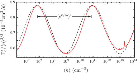
Figure 2: Three-body decay rate, $\Gamma^{*}_{3}$, for ⁸⁵Rb at $|a|=\infty$ as a function of the average density, $\langle n\rangle$. This figure display the $\langle n^{2/3}\rangle$ scaling of the decay rate as well as the appearance of log-periodic oscillations associated with Efimov physics. Resonances at higher $\langle n\rangle$ occur when the initial state is degenerate with one of the possibly weakly-coupled final states in our model. Dashed black curve is the fitting function in Eq. (8).

Besides the three-body eigenenergies, our model also provides wave functions that determine various properties of the quenched system. After quenching to the unitary regime, the time evolution of the three-body system is described by the projected three-body wave function,

$$\Psi(R,\Omega,t)=\sum_{\beta}c_{\beta}^{(u)}\psi_{\beta}^{(u)}(R,\Omega)e^{-i(E_{\beta}-i\Gamma_{\beta}/2)t/\hbar},$$ (6)

which is a superposition of states at unitary, $\psi_{\beta}^{(u)}$, with coefficients determined from their overlap with the initial state, $c_{\beta}^{(u)}=\langle\psi^{(u)}_{\beta}|\psi_{i}\rangle$. Within our local model, however, the wave function in Eq. (6) can only be expected to qualitatively represent the actual many-body system for $t<t_{n}$, since beyond this time scale genuine many-body effects should become important. Figure 1(c) shows the population at unitarity, $|c_{\beta}|^{2}$, for various states as a function of $n_{\rm lo}$. We observe that the population of a given state becomes substantial when its energy or size is in the vicinity of the density-derived scales of the unitary Bose gas ($\epsilon_{n}$ and $k^{-1}_{n}$, respectively).

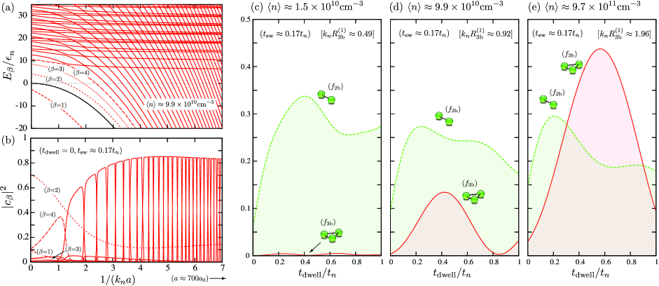
Figure 3: (a) Three-body energy spectrum for $\langle n\rangle\approx 9.9\times 10^{10}$cm^-3 within a range of $a$ relevant for the ⁸⁵Rb experiment. Black solid line corresponds to the energy of the (free-space) diatomic state ($\hbar^{2}/ma^{2}$). (b) Corresponding change of population during the field sweep ($t_{\rm sw}\approx 0.17t_{n}$) obtained immediately after the quench ($t_{\rm dwell}=0$). (c)-(e) Population fraction of diatomic and Efimov states formed as a function of $t_{\rm dwell}$ illustrating the enhancement of Efimov state formation as the density approaches the characteristic value $\langle n_{1}^{*}\rangle\approx 5.2\times 10^{10}$cm^-3 [Eq. (9)] or, equivalently, when $k_{n}R_{\rm 3b}\approx 0.78(2)$ colussi2018PRL .

The above results suggest that Efimov physics may manifest in the density dependence of relevant observables since the atomic density sets the energy and length scales of the gas. We first focus on the three-body decay rates, which can be simply evaluated within our model from sykes2014PRA

$$\Gamma_{3}^{*}=-\lim_{t\rightarrow 0}\frac{\dot{n}(t)}{n(t)}=\sum_{\beta}|c_{\beta}^{(u)}(n_{\rm lo})|^{2}\frac{\Gamma_{\beta}(n_{\rm lo})}{\hbar},$$ (7)

where $n(t)=n_{\rm lo}|\langle\Psi(R,\Omega,t)|\Psi(R,\Omega,t)\rangle|$. In a local density model, the decay rate in Eq. (7) is averaged over the local density $n_{\rm lo}$. Using a Thomas-Fermi density profile, our numerical calculations indicate that the averaged rate is well approximated (within no more than 4%) by replacing $n_{\rm lo}$ with the corresponding average density $\langle n\rangle$ in Eq. (7). Our results for the three-body decay rate for the quenched unitary Bose gas are shown in Fig. S.1, covering a broad range of densities. We find the expected $\langle n^{2/3}\rangle$ scaling werner2012PRA ; smith2014PRL ; klauss2017PRL but also log-periodic oscillations that originate from the increase of an Efimov state population whenever its binding energy is comparable to $\epsilon_{n}$ (see Fig. 1). We fit these oscillations as

$$\Gamma_{3}^{*}\approx\eta\frac{\hbar}{m}\left[A+B\sin^{2}\Big{(}s_{0}\ln\scalebox{1.1}{$\frac{\langle n\rangle^{1/3}}{r_{\rm vdW}^{-1}}$}+\phi\Big{)}\right]\langle n^{2/3}\rangle$$ (8)

where $A\approx 15.9$, $B\approx 8.80$, and $\phi\approx 1.61$ —see dashed black curve in Fig. S.1. Our numerical calculations, although largely log-periodic, are slightly asymmetric. The results shown in Fig. S.1 have roughly 40% lower amplitude than the experimental decay rate for ⁸⁵Rb klauss2017PRL , however, the oscillation phase is consistent with preliminary experimental observations klauss2017PhD . While our results account for losses at unitarity only, the experimental data was obtained after a $B$-field sweep to weak interactions klauss2017PRL , thus allowing for additional atom loss. Nevertheless, the existence of the log-periodic oscillations in Fig. S.1, with a substantial amplitude, violates the universality hypothesis ho2004PRL , in which all observables related to the unitary Bose gas should scale continuously as powers of $n$. Equation (8) depends only on the system parameters $r_{\rm vdW}$ and $\eta$ for a particular atomic species.

We now shift our focus to the dynamical formation of weakly bound diatomic and Efimov states in quenched unitary Bose gases. In fact, in the recent ⁸⁵Rb experiment of Ref. klauss2017PRL a population of such few-body bound states was obtained by quenching the system to unitary, evolving for a time $t_{\rm dwell}$, and subsequently sweeping the system back to weaker interactions ($a\approx 700a_{0}$) within a time $t_{\rm sw}$. There is still, however, much to be understood on the dependence of populations on the various parameters ($n$, $t_{\rm dwell}$, and $t_{\rm sw}$) and the possible connections to the non-equilibrium dynamics in the unitary regime. In order to address some of these questions we focus initially on the case $t_{\rm sw}\ll t_{n}$, where ramping effects are minimized, and solve the time-dependent three-body Schrödinger equation following the same experimental protocol of Ref. klauss2017PRL described above —see also Refs. SupMat ; baekhoj2014JPB . Figure 3(a) shows the three-body energy spectrum for a given density and for a range of $a$ relevant for the ⁸⁵Rb experiment. For this particular density, $\langle n\rangle\approx 9.9\times 10^{10}$cm^-3, only the ground- [$\beta=0$, not shown in Fig. 3(a)] and first-excited Efimov states ($\beta=1$) have sizes smaller than the average interatomic distance. The black solid line in Fig. 3(a) is the energy of the (free-space) diatomic state, $-\hbar^{2}/ma^{2}$, while the red curves following along this threshold correspond to atom-diatom states, and those following along the $E=0$ threshold correspond to three-atom states. Figure 3(b) shows the population changes during the sweep of the interactions ($t_{\rm sw}\approx 0.17t_{n}$) from $|a|=\infty$ to $a\approx 700a_{0}$, for a case in which the system is not held in the unitary regime ($t_{\rm dwell}=0$). Whenever $t_{\rm dwell}=0$, the population of few-body bound states develops entirely during the interaction sweep. To quantify the population dynamics, we define the fraction of formed two-body states, $f_{\rm 2b}=(2/3)\sum_{\beta}|c_{\beta}|^{2}$, and Efimov states, $f_{\rm 3b}=\sum_{\beta}|c_{\beta}|^{2}$, after the sweep SupMat . For the parameters of Fig. 3(b), we find that $f_{\rm 2b}$ and $f_{\rm 3b}$ are approximately $0.095$ and $0.004$, respectively, with the remaining fraction of atoms unbound.

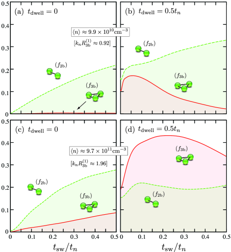
Figure 4: Dependence of $f_{\rm 2b}$ and $f_{\rm 3b}$ on $t_{\rm sw}$ for (a)-(b) $\langle n\rangle\approx 9.9\times 10^{10}$cm^-3 and (c)-(d) $9.7\times 10^{11}$cm^-3. For $t_{\rm dwell}=0$, the dependence on $t_{\rm sw}$ is well described by the Landau-Zener results (see text) while for $t_{\rm dwell}=0.5t_{n}$ [(b) and (d)] the growth of correlations lead to the enhancement of the trimer population and a departure from the Landau-Zener results.

To explore how the time-evolution of the system at unitarity impacts the formation of two- and three-body bound states, we study their dependence on $t_{\rm dwell}$ over a range of atomic densities [see shaded region in Fig. 1(b)]. Figure 3(c) shows that for a relatively low density where, although $f_{\rm 2b}$ grows fast and reaches appreciable values, $f_{\rm 3b}$ still remains negligible for all $t_{\rm dwell}$. A larger population of Efimov states, however, is observed for higher densities [see Figs. 3(d) and (e), and Ref. SupMat .] In general, we find that for short-times $f_{\rm 2b}\propto t_{\rm dwell}$ and $f_{\rm 3b}\propto t_{\rm dwell}^{2}$, consistent with the early-time growth of two- and three-body correlations found in Ref. colussi2018PRL . Also, in Ref. colussi2018PRL , it was observed that at early-times the largest enhancement of three-body correlations occurred at densities where the average interatomic distance is comparable to the size of an Efimov state. More precisely, this occured when $k_{n}R_{\rm 3b}=0.74(5)$, associated with a characteristic density value

$$\langle{n_{j}^{*}}\rangle\approx 0.41\frac{(3/2)^{1/2}}{4\pi^{2}(1+s_{0}^{2})^{3/2}}\frac{\kappa_{*}^{3}}{(e^{\pi/s_{0}})^{3j}}.$$ (9)

For the range of densities explored in the ⁸⁵Rb experiment klauss2017PRL the relevant characteristic density is $\langle{n_{1}^{*}}\rangle\approx 5.2\times 10^{10}$cm^-3. In fact, Figs. 3 (c)-(e) display a marked change in the dynamics of $f_{\rm 3b}$ as $\langle{n_{1}^{*}}\rangle$ is approached from below and then exceeded. In Figs. 3 (c)-(e) we also display the corresponding values for $k_{n}R_{\rm 3b}$. For densities beyond $\langle{n_{1}^{*}}\rangle$ (see also Ref. SupMat ) the population of Efimov states is clearly enhanced and can be attributed to the growth of few-body correlations colussi2018PRL . Within our model, such enhancement is also consistent with the increase of population of the first-excited Efimov state at unitarity [see Fig. 1(b)].

Correlation growth can also be further studied by investigating the dependence of the populations on $t_{\rm sw}$, shown in Fig. 4 for two densities and for $t_{\rm dwell}=0$ and $0.5t_{n}$. For $t_{\rm dwell}=0$ [Figs. 4(a) and (c)], i.e., in absence of time evolution at unitarity and the corresponding growth of correlations, the dependence of the populations on $t_{\rm sw}$ is well described by the Landau-Zener result: $f=f_{m}(1-e^{-t_{\rm sw}/t_{m}})$, where $f_{m}$ is the final population and $t_{m}$ the time scale related to the strength of the couplings between the states involved in the process stecher2007PRL ; clark1979PLA . These findings are drastically changed as the system is allowed to evolve at unitarity, coinciding with the growth of few-body correlations colussi2018PRL . In that case, as shown in Figs. 4(b) and (d), the population dynamics departs from the Landau-Zener results. For $t_{\rm dwell}\neq 0$, there is a clear enhancement of $f_{\rm 3b}$ —even at $t_{\rm sw}=0$— which, in some cases [Fig. 4(d) and Ref. SupMat ], can lead to a population of Efimov states exceeding that of diatomic states.

In summary, solving the three-body problem in a local harmonic trap, designed to reflect density effects, we highlight the importance of Efimov physics in quenched unitary Bose gases. Within our model, the continuous scaling invariance of unitary Bose gases is violated in relevant three-body observables. In the three-body decay rates, this violation manifests through the appearance of log-periodic oscillations characteristic of the Efimov effect. In the early-time population growth of Efimov states after the system is swept away from unitarity it manifests through a marked change in dynamics as the density exceeds a characteristic value corresponding to a length scale matching that of the Efimov state size and interparticle spacing. Furthermore, our study characterizes the growth of correlations at unitarity through the early-time dynamics of the population of diatomic and Efimov states. This is shown to be qualitatively consistent with the early-time growth of two- and three-body correlations at unitarity observed in Ref. colussi2018PRL . Moreover, we find that the departure from the Landau-Zener results for the populations in the non-equilibrium regime can also be associated with the increase of correlations in the system. An experimental study of the predictions of our model is within the range of current quenched unitary Bose gas experiments.

The authors thank E. A. Cornell, C. E. Klauss, J. L. Bohn, J. P. Corson, D. Blume and S. Kokkelmans for extensive and fruitful discussions. J. P. D. acknowledges support from the U.S. National Science Foundation (NSF), Grant PHY-1607204, and from the National Aeronautics and Space Administration (NASA). V.E.C. acknowledges support from the NSF under Grant PHY-1734006 and by Netherlands Organization for Scientific Research (NWO) under Grant 680-47-623.

I Supplementary Material

I.1 A. Lifetime of three-body states

Figure S.1(a) shows the energy levels, $E_{\beta}$, of three-identical bosons at $|a|=\infty$ as a function of local density $n_{\rm lo}$, related to the local harmonic trap used in our model [see Eqs. (3) and (4) of the main text]. For the present study, atoms interact via a Lennard-Jones potential, $v(r)=-C_{6}/r^{6}(1-\lambda^{6}/r^{6})$, where $C_{6}$ is the dispersion coefficient chin2010RMP , and set $\lambda\approx 0.9197\>r_{\rm vdW}$ to give $|a|=\infty$, such that only a single (zero-energy) $s$-wave dimer can exist. (For ⁸⁵Rb, $r_{\rm vdW}\approx 82.5a_{0}$ kempen2002PRL ; chin2010RMP and atomic mass $m\approx 1.56\times 10^{5}$a.u..) In that case, the width $\Gamma_{\beta}$ of three-body states is obtained by introducing a purely hyperradial absorbing potential $iV_{\rm ab}(R)/2$, mimicking decay to deeply bound molecular states. The resulting width of the states can be then determined by

$$\Gamma_{\beta} =\langle\psi_{\beta}|V_{\rm ab}(R)|\psi_{\beta}\rangle$$

$$=\sum_{\nu}\langle F_{\beta\nu}(R)|V_{\rm ab}(R)|F_{\beta\nu}(R)\rangle,$$ (S.1)

where $\psi_{\beta}$ is the total three-body wave function for the state $\beta$ and $F_{\beta\nu}$ the corresponding hyperradial amplitude for channel $\nu$ [Eqs. (1) and (2)].

Our definition of the width in Eq. (S.1) is in close analogy to other proposed ways to estimate the width of Efimov states braaten2006PRep ; werner2006PRL because it is also based on the probability to find atoms at short-distances, where inelastic transitions to deeply bound states occur. In our calculations we have used $V_{\rm ab}(R)=D\exp[-R^{2}/(2\rho^{2})]$, with the parameters $D$ and $\rho$ adjusted to reproduce the expected width via the relation

$$\Gamma_{0}=\frac{4\eta}{s_{0}}|E_{0}|,$$ (S.2)

where $E_{0}$ is the energy of the Efimov ground state in free space at $|a|=\infty$. In our present study we assume $\eta=0.06$. This is consistent with the observed value for ⁸⁵Rb wild2012PRL , and vary $\rho$ and $D$ until Eq. (S.2) is satisfied. This is achieved for the choice of parameters: $\rho=2r_{\rm vdW}$ and $D=1.8\times 10^{-1}\hbar^{2}/mr_{\rm vdW}^{2}$. The resulting lifetimes $\tau_{\beta}=\hbar/\Gamma_{\beta}$ of the three-identical bosons states from Fig. S.1(a) are shown in Fig. S.1(b). Away from $|a|=\infty$, the same parameters $\rho$ and $D$ lead to a lifetime of $109\mu$s for the first-excited Efimov state, consistent with the observations of Ref. klauss2017PRL , indicating the validity of our decay model [Eq. (S.1)] for other values of $a$.

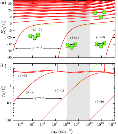
Figure S.1: (a) Three-body energies, $E_{\beta}$, and (b) corresponding lifetimes, $\tau_{\beta}$, of three-identical bosons at $|a|=\infty$ as a function of the local density, $n_{\rm lo}$ or, equivalently, as a function of the strength of the local harmonic trap in Eq. (4). The dashed green lines represent the energies and lifetimes of Efimov states in free space.

I.2 B. Field sweep of interactions

In the ⁸⁵Rb experiment with unitary Bose gases klauss2017PRL , a sequence of magnetic field ramps has been implemented in order to study the dynamics of the system. Reference klauss2017PRL uses the 155G Feshbach resonance with parameters: $B_{0}\approx 155.041$G, $a_{bg}\approx-443a_{0}$ and $\Delta\approx 10.71$G claussen2003PRA , where $B_{0}$ is the resonance position, $a_{bg}$ the background scattering length and $\Delta$ the resonance width. The ramping scheme is shown in Fig. S.2. At $t=0$ the system is initially in the weakly interacting ground state, $B$ is then quickly ramped from a value where $a\approx 150a_{0}(=a_{i})$ ($B\approx B_{0}+8G$) to a value in which $|a|=\infty$ ($B=B_{0}$), thus quenching the interactions. The shaded region in Fig. S.2 represents the range of $B$ where $n|a|^{3}>1$. The system is then held at unitarity for a variable time $t_{\rm dwell}$ and then slowly swept away to weaker interactions ($a_{f}\approx 700a_{0}$, or $B\approx 159$G) over a time $t_{\rm sw}$. For the Lennard-Jones potential we use (see above) the values of $\lambda$ producing $a_{i}\approx 0.7725\>r_{\rm vdW}$ and $a_{f}\approx 0.8922\>r_{\rm vdW}$. Once the system is swept away from unitarity, the population of weakly bound diatomic and Efimov states is determined klauss2017PRL .

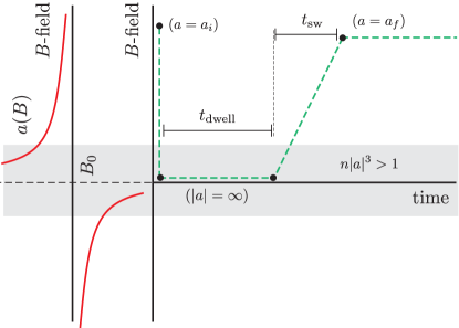
Figure S.2: Magnetic field ramp scheme implemented in the ⁸⁵Rb experiment. Initially ($t=0$), the system is rapidly quenched by quickly changing the magnetic field from $a\approx 150a_{0}(=a_{i})$ to $|a|=\infty$. The the system is held at unitarity for a variable time $t_{\rm dwell}$. Finally, the system is slowly swept away from unitarity to weaker interactions ($a_{f}\approx 700a_{0}$) over a time $t$.

There are three distinct regions in Fig. S.2 where the three-body physics is studied within our model. For $t<0$, the three-body system is in the lowest trapped eigenstate of the Hamiltonian for weak interactions ($a=a_{i}$) [lowest positive energy state on the far right of Fig. 3(a)]. The total wave function for $t<0$ is given by

$$\Psi_{i}(R,\Omega,t)=\psi_{i}(R,\Omega)e^{-iE_{i}t/\hbar}.$$ (S.3)

At $t=0$, the interaction is quenched and the total wave function is given by a superposition of trapped three-body states at unitarity [see states on the left of Fig. 3(a)],

$$\Psi_{u}(R,\Omega,t)=\sum_{\beta}c_{\beta}^{(u)}\psi_{\beta}^{(u)}(R,\Omega)e^{-i(E_{\beta}^{(u)}-i\Gamma_{\beta}^{(u)}/2)t/\hbar},$$ (S.4)

with coefficients $c_{\beta}$

$$c_{\beta}^{(u)} =\big{\langle}\psi^{(u)}_{\beta}\big{|}\Psi_{i}(t=0)\big{\rangle}$$

$$=\sum_{\nu\nu^{\prime}}\int[F_{\nu\beta}^{(u)}(R)]^{*}F_{\nu^{\prime}\beta_{i}}^{(i)}(R)dR$$

$$~{}~{}~{}~{}~{}~{}\times\int[\Phi_{\nu}^{(u)}(R;\Omega)]^{*}\Phi_{\nu^{\prime}}^{(i)}(R;\Omega)d\Omega.$$ (S.5)

This determines the time evolution of the system until $t=t_{\rm dwell}$. For $t_{\rm dwell}\leq t\leq t_{\rm dwell}+t_{\rm sw}$, interactions are slowly swept from $|a|=\infty$ to $a_{f}$ [from left to right of Fig. 3(a)], and the time evolution of the system is dictated by the time-dependent Schrödinger equation:

$$H(R,\Omega,t)\Psi_{\rm sw}(R,\Omega,t)=i\hbar\frac{\partial}{\partial t}\Psi_{\rm sw}(R,\Omega,t).$$ (S.6)

For $t\geq t_{\rm dwell}+t_{\rm sw}$, the time evolution is given by

$$\Psi_{f} (R,\Omega,t)=$$

$$\sum_{\beta}c_{\beta}^{(f)}\psi_{\beta}^{(f)}(R,\Omega)e^{-i(E_{\beta}^{(f)}-i\Gamma_{\beta}^{(f)}/2)(t-t_{\rm dwell}-t_{\rm sw})/\hbar}.$$ (S.7)

We then determine the final state populations resulting from the ramping scheme in Fig. S.2 from

$$|c_{\beta}^{(f)}|^{2} =|\big{\langle}\psi^{(f)}_{\beta}\big{|}\Psi_{\rm sw}(t=t_{\rm dwell}+t_{\rm sw})\big{\rangle}|^{2}.$$ (S.8)

I.3 C. SVD approximation in time

Numerically solving the time-dependent Schrödinger equation (S.6) is crucial to studying the ramping scheme in Fig. S.2. However, from the variation of the energy spectrum in Fig. 3 in time as $a$ changes, it is clear that an adiabatic approach in time will encounter numerical instabilities due to sharp avoid-crossings. In order to circumvent such issues, we extend the SVD approach of Ref. wang2011PRA to the time domain, in a similar fashion to Ref. baekhoj2014JPB .

In our SVD formulation in the time domain, the total wave function [solution of Eq. (S.6)] is expanded in terms of the DVR basis lill1982CPL ; rescino2000PRA , $\pi_{j}(t)$, in the following way:

$$\Psi(R,\Omega,t)=\sum_{j\beta}C_{j\beta}\pi_{j}(t)\psi^{(t_{j})}_{\beta}(R,\Omega),$$ (S.9)

where $\psi^{(t)}_{\beta}$ is the eigenstate of $H$ at time $t$, with energy given by $E_{\beta}(t)$. We determine the $C_{j\beta}$ coefficients for a given initial condition. Various properties of the DRV basis derived below are needed to derive the form of the Hamiltonian matrix elements wang2011PRA .

The DVR basis functions $\pi_{j}(t)$ are defined by the Gauss-Lobatto quadrature points $x_{j}$ and weights $w_{j}$ manolopoulos1998cpl . The Gauss-Lobatto quadrature approximates integrals of a function $g\left(t\right)$ as

$$\int_{t_{1}}^{t_{N}}g(t)dt\cong\sum_{j=1}^{N}g(t_{j})\widetilde{w}_{j},$$ (S.10)

where $N$ is the number of quadrature points and

$$\widetilde{w}_{j}=\frac{t_{N}-t_{1}}{2}w_{j},~{}~{}~{}t_{j}=\frac{t_{N}-t_{1}}{2}x_{j}+\frac{t_{N}+t_{1}}{2}.$$ (S.11)

Equation (S.10) is exact for polynomials of degree less than or equal to $2N-1$. The DVR basis functions and their derivatives are constructed based on values for $t_{j}$ and $\widetilde{w}_{j}$ as following

$$\pi_{j}(t) = \sqrt{\frac{1}{\widetilde{w}_{j}}}\prod\limits_{k\neq j}^{N}{\frac{{t-t_{k}}}{{t_{j}-t_{k}}}},$$ (S.12)

$$\frac{d}{dt}\pi_{j}(t) = \sqrt{\frac{1}{\widetilde{w}_{j}}}\sum_{l\neq j}^{N}\bigg{(}\frac{1}{t-t_{l}}\prod\limits_{k\neq j,l}^{N}{\frac{{t-t_{k}}}{{t_{j}-t_{k}}}}\bigg{)}.$$ (S.13)

This leads to important properties for calculating matrix elements at the quadrature points,

$$\pi_{j}(t_{i}) = \sqrt{\frac{1}{\widetilde{w}_{j}}}\delta_{ij}~{}~{}~{}(\forall~{}i,j),$$ (S.14)

$$\pi_{j}^{\prime}(t_{i}) = \sqrt{\frac{1}{\widetilde{w}_{j}}}\frac{1}{t_{j}-t_{i}}\prod\limits_{k\neq i,j}^{N}{\frac{{t_{i}-t_{k}}}{{t_{j}-t_{k}}}}~{}~{}~{}(i\neq j),$$ (S.15)

$$\pi_{j}^{\prime}(t_{i}) = \sqrt{\frac{1}{\widetilde{w}_{j}}}\frac{\delta_{jN}-\delta_{j1}}{2\widetilde{w}_{j}}~{}~{}~{}(i=j).$$ (S.16)

Property (S.14), for instance, can be used to calculate integrals involving the DVR basis and an arbitrary function $F(t)$ in a trivial way,

$$\int_{t_{a}}^{t_{b}}\pi_{j}(t)F(t)\pi_{k}(t)dt \cong \sum_{l=1}^{N}\pi_{j}(t_{l})F(t_{l})\pi_{k}(t_{l})\widetilde{w}_{l}$$ (S.17)

$$= F(t_{j})\delta_{jk},$$

which is usually called the DVR approximation.

Now, substituting Eq. (S.9) in Eq. (S.6), and projecting out in the basis $\pi_{i}(t)\psi_{\alpha}^{(t_{i})}$, yields a linear system of equations for the coefficients $C_{j\beta}$,

$$\sum_{j\beta}\left(\widetilde{H}_{i\alpha,j\beta}-\widetilde{L}_{i\alpha,j\beta}\right)C_{j\beta}=0.$$ (S.18)

Equivalently, this system of equations can be written in the matrix form $\widetilde{H}\vec{C}=\widetilde{L}\vec{C}$, with matrix elements given by

$$\widetilde{H}_{i\alpha,j\beta} = E_{\beta}(t_{i})\delta_{\alpha\beta}\delta_{ij}$$ (S.19)

$$- \frac{i\hbar}{2}\int_{t_{a}}^{t_{b}}\left[\pi_{i}(t)\frac{d}{dt}\pi_{j}(t)-\frac{d}{dt}\pi_{i}(t)\pi_{j}(t)\right]dt~{}O^{i\alpha}_{j\beta}$$

$$= E_{\beta}(t_{i})\delta_{\alpha\beta}\delta_{ij}$$

$$- \frac{i\hbar}{2}\left[\sqrt{\widetilde{w}_{i}}\pi^{\prime}_{j}(t_{i})-\sqrt{\widetilde{w}_{j}}\pi^{\prime}_{i}(t_{j})\right]O^{i\alpha}_{j\beta},$$

and

$$\widetilde{L}_{i\alpha,j\beta} = \frac{i\hbar}{2}\left[\pi_{i}(t_{b})\pi_{j}(t_{b})-\pi_{i}(t_{a})\pi_{j}(t_{a})\right]O^{i\alpha}_{j\beta}$$ (S.20)

$$= \frac{i\hbar}{2}\left(\frac{\delta_{iN}\delta_{jN}}{\widetilde{w}_{N}}-\frac{\delta_{i1}\delta_{j1}}{\widetilde{w}_{1}}\right)\delta_{\alpha\beta},$$

where the overlapping matrix is calculated from

$$O^{i\alpha}_{j\beta}=\int\psi^{(t_{i})*}_{\alpha}(R,\Omega)\psi^{(t_{j})}_{\beta}(R,\Omega)d\Omega dR.$$ (S.21)

This problem can be solved by writing Eq. (S.18) as $\vec{C}=(\widetilde{H}^{-1}L)\vec{C}$. Due to the form of the matrix $L$ [Eq. (S.20)], however, the coefficients $\vec{C}$ can be written as

$$C_{i\alpha} = \sum_{j\beta}\left(\widetilde{H}^{-1}L\right)_{i\alpha,j\beta}C_{j,\beta}$$ (S.22)

$$= \sum_{\beta}(R_{iN})_{\alpha\beta}C_{N\beta}-\sum_{\beta}(R_{i1})_{\alpha\beta}C_{1\beta},$$

where $R_{ij}$ is the matrix defined as

$$(R_{ij})_{\alpha\beta}=\frac{i\hbar}{2\widetilde{w}_{j}}(\widetilde{H}^{-1})_{i\alpha,j\beta}.$$ (S.23)

Now, writing Eq. (S.22) in the matrix notation,

$$\vec{C}_{i} = R_{iN}\vec{C}_{N}-R_{i1}\vec{C}_{1},$$ (S.24)

where $\vec{C}_{i}$ is a vector of components $C_{i\alpha}$, with $\vec{C}_{1}$ determined by the initial condition (see below) and $\vec{C}_{N}$ by

$$\vec{C}_{N} = (R_{1N})^{-1}(\mathbb{1}+R_{11})\vec{C}_{1},$$ (S.25)

obtained by making $i=1$ in Eq. (S.24). Putting together these results we finally obtain

$$\vec{C}_{i} = \left[R_{iN}(R_{1N})^{-1}(\mathbb{1}+R_{11})-R_{i1}\right]\vec{C}_{1},$$ (S.26)

determining the coefficients $C_{i\beta}$ in Eq. (S.9) for all grid points in the interval $t\in\left[t_{1},t_{N}\right]$. An alternative solution can be obtained by setting $i=N$ in Eq. (S.24). In that case, we obtain

$$\vec{C}_{i} = -\left[R_{iN}(\mathbb{1}-R_{NN})^{-1}R_{N1}+R_{i1}\right]\vec{C}_{1}.$$ (S.27)

We have observed that the numerical calculations are more stable by choosing the propagation scheme defined by Eq. (S.27).

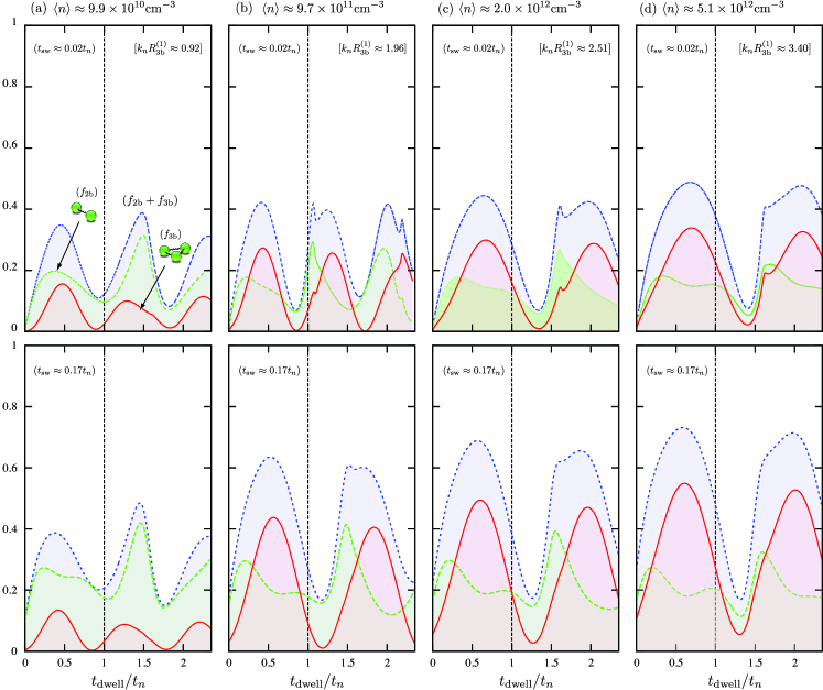
Figure S.3: Dependence of $f_{\rm 2b}$, $f_{\rm 3b}$, and $f_{\rm 2b}+f_{\rm 3b}$, on $t_{\rm dwell}$ for various densities, satisfying the condition $k_{n}R_{\rm 3b}>0.74(5)$ colussi2018PRL , and $t_{\rm sw}=0.02t_{n}$ and $0.17t_{n}$ (top and bottom panels, respectively). In all cases, the $t_{\rm dwell}$ dependence is shown for times beyond the range of validity of our approach ($t<t_{n}$) to illustrate the time periodicity implied by our local harmonic trap.

Applying this method to the current problem, we find that dividing the time domain into sectors is advantageous. Within the first sector, the ${C}_{1\beta}$ coefficients correspond to the initial condition at $t=t_{\rm dwell}$ determined by simply equating Eq. (S.4) and Eq. (S.9) and making use the property of the DVR basis in Eq. (S.14). This leads to

$$C_{1\beta}=\sqrt{\widetilde{w}_{1}}c_{\beta}^{(u)}e^{-i(E_{\beta}^{(u)}-i\Gamma_{\beta}^{(u)})t_{\rm dwell}/\hbar}.$$ (S.28)

The coefficients corresponding to the last point within the first sector, $C_{N\beta}$, serve as the initial condition for the propagation within the next sector. This procedure continues until the last sector, with the last point corresponding to $t_{N}=t_{\rm dwell}+t_{\rm sw}$. From this point, we determine the coefficients of the final total wavefunction in Eq. (S.7) as

$$c_{\beta}^{(f)}=C_{N\beta}/\sqrt{\widetilde{w}_{N}}.$$ (S.29)

As a result, the final population of a state $\beta$ is simply determined by calculating $|c_{\beta}|^{2}$. In order to associate these populations to the actual populations of diatomic and triatomic states, the nature of the particular $\beta$ states must be accounted. For instance, $\beta$ states whose energies follow the black solid line in Fig. 3(a) ($E_{\beta}>-\hbar^{2}/ma^{2}$) represent an atom-diatom state. In that case, the corresponding population of diatomic molecules is given by $f_{\rm 2b}=(2/3)\sum_{\beta}|c_{\beta}|^{2}$. For triatomic states, with energies $E_{\beta}<-\hbar^{2}/ma^{2}$, the population is determined by $f_{\rm 3b}=\sum_{\beta}|c_{\beta}|^{2}$.

I.4 D. Populations of diatomic and Efimov states

Figures S.3 and S.4 display various calculations for the population of weakly bound diatomic and Efimov states that support and complement the conclusions of the main text. In Fig. S.3 we show the dependence of $f_{\rm 2b}$, $f_{\rm 3b}$, and $f_{\rm 2b}+f_{\rm 3b}$, on $t_{\rm dwell}$ for two values of $t_{\rm sw}$ and densities $k_{n}R^{(1)}_{\rm 3b}>0.74(5)$, exceeding the density where maximal early-time enhancement of three-body correlations was observed in Ref.  colussi2018PRL . In all cases shown in Fig. S.3 we have displayed the $t_{\rm dwell}$ dependence for times beyond the range of validity of our approach ($t<t_{\mathrm{n}}$) in order to illustrate the time periodicity due to the local harmonic trap in our model. As expected for short sweep times, our results for $t_{\rm sw}=0.02t_{n}$ [top panels of Figs. S.3(a)-(d)] clearly show that populations are negligible for $t_{\rm dwell}\ll t_{n}$. However, for a finite value of $t_{\rm dwell}$ the populations of both diatomic and triatomic states become substantial after evolving at unitary while correlations develop colussi2018PRL . For longer sweep times, $t_{\rm sw}=0.17t_{n}$ [bottom panels of Figs. S.3(a)-(d)], a more substantial population is observed for $t_{\rm dwell}\ll t_{n}$. This indicates that $t_{\rm sw}=0.17t_{n}$ is slow enough to produce populations even if the system is does not evolve at unitarity.

Figure S.4 shows the dependence of $f_{\rm 2b}$ and $f_{\rm 3b}$, as well as $f_{\rm 2b}+f_{\rm 3b}$, on $t_{\rm sw}$ for various densities and three values of $t_{\rm dwell}$. These results complement our discussion on the breakdown of the Landau-Zener model in the main text. For a two-level system, the Landau-Zener model predicts that after sweeping the interactions across an avoided-crossing the final state population is determined by $f=f_{m}(1-e^{-t_{\rm sw}/t_{m}})$, where $f_{m}$ is the final population and $t_{m}$ the time scale related to the strength of the couplings between the states involved in the process stecher2007PRL ; clark1979PLA . The results for $t_{\rm dwell}=0$, displayed in the top panels of Figs. S.4(a)-(d), agree well with the Landau-Zener formula —this agreement tends to deteriorate as the density increases. For $t_{\rm dwell}\neq 0$ [middle and bottom panels of Figs. S.4(a)-(d)], however, our results depart from the Landau-Zener formula. This departure coincides with the growth of few-body correlations colussi2018PRL , thus providing an alternative way to characterize such phenomena.

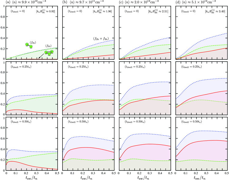
Figure S.4: Dependence of $f_{\rm 2b}$, $f_{\rm 3b}$, and $f_{\rm 2b}+f_{\rm 3b}$, on $t_{\rm sw}$ for various densities and $t_{\rm dwell}=0$, $0.25t_{n}$, and $0.50t_{n}$ (top, middle, and bottom panels, respectively).

References

- (1) R. J. Fletcher, A. L. Gaunt, N. Navon, R. P. Smith, and Z. Hadzibabic, “Stability of a unitary bose gas,” Phys. Rev. Lett., vol. 111, p. 125303, 2013.
- (2) B. S. Rem, A. T. Grier, I. Ferrier-Barbut, U. Eismann, T. Langen, N. Navon, L. Khaykovich, F. Werner, D. S. Petrov, F. Chevy, and C. Salomon, “Lifetime of the bose gas with resonant interactions,” Phys. Rev. Lett., vol. 110, p. 163202, 2013.
- (3) P. Makotyn, C. E. Klauss, D. L. Goldberger, E. A. Cornell, and J. D. S., “Universal dynamics of a degenerate unitary bose gas,” Nat. Phys., vol. 10, p. 116, 2014.
- (4) U. Eismann, L. Khaykovich, S. Laurent, I. Ferrier-Barbut, B. S. Rem, A. T. Grier, M. Delehaye, F. Chevy, C. Salomon, L.-C. Ha, and C. Chin, “Universal loss dynamics in a unitary bose gas,” Phys. Rev. X, vol. 6, p. 021025, 2016.
- (5) F. Chevy and C. Salomon, “Strongly correlated bose gases,” J. Phys. B, vol. 49, no. 19, p. 192001, 2016.
- (6) R. J. Fletcher, R. Lopes, J. Man, N. Navon, R. P. Smith, M. W. Zwierlein, and Z. Hadzibabic, “Two and three-body contacts in the unitary bose gas,” Science, vol. 355, p. 377, 2017.
- (7) S. Laurent, M. Pierce, M. Delehaye, T. Yefsah, F. Chevy, and C. Salomon, “Connecting few-body inelastic decay to quantum correlations in a many-body system: A weakly coupled impurity in a resonant fermi gas,” Phys. Rev. Lett., vol. 118, p. 103403, 2017.
- (8) C. E. Klauss, X. Xie, C. Lopez-Abadia, J. P. D’Incao, Z. Hadzibabic, D. S. Jin, and E. A. Cornell, “Observation of efimov molecules created from a resonantly interacting bose gas,” Phys. Rev. Lett., vol. 119, p. 143401, 2017.
- (9) C. Eigen, J. A. P. Glidden, R. Lopes, N. Navon, Z. Hadzibabic, and R. P. Smith, “Universal scaling laws in the dynamics of a homogeneous unitary bose gas,” Phys. Rev. Lett., vol. 119, p. 250404, 2017.
- (10) R. J. Fletcher, J. Man, R. Lopes, P. Christodoulou, J. Schmitt, M. Sohmen, N. Navon, R. P. Smith, and Z. Hadzibabic, “Elliptic flow in a strongly-interacting normal bose gas,” arxiv:1803.06338, 2018.
- (11) T.-L. Ho, “Universal thermodynamics of degenerate quantum gases in the unitarity limit,” Phys. Rev. Lett., vol. 92, p. 090402, Mar 2004.
- (12) J. M. Diederix, T. C. F. van Heijst, and H. T. C. Stoof, “Ground state of a resonantly interacting bose gas,” Phys. Rev. A, vol. 84, p. 033618, Sep 2011.
- (13) W. Li and T.-L. Ho, “Bose gases near unitarity,” Phys. Rev. Lett., vol. 108, p. 195301, May 2012.
- (14) S.-J. Jiang, W.-M. Liu, G. W. Semenoff, and F. Zhou, “Universal bose gases near resonance: A rigorous solution,” Phys. Rev. A, vol. 89, p. 033614, Mar 2014.
- (15) S. Laurent, X. Leyronas, and F. Chevy, “Momentum distribution of a dilute unitary bose gas with three-body losses,” Phys. Rev. Lett., vol. 113, p. 220601, 2014.
- (16) X. Yin and L. Radzihovsky, “Quench dynamics of a strongly interacting resonant bose gas,” Phys. Rev. A, vol. 88, p. 063611, Dec 2013.
- (17) A. G. Sykes, J. P. Corson, J. P. D’Incao, A. P. Koller, C. H. Greene, A. M. Rey, K. R. A. Hazzard, and J. L. Bohn, “Quenching to unitarity: Quantum dynamics in a three-dimensional bose gas,” Phys. Rev. A, vol. 89, p. 021601, 2014.
- (18) M. Rossi, L. Salasnich, F. Ancilotto, and F. Toigo, “Monte carlo simulations of the unitary bose gas,” Phys. Rev. A, vol. 89, p. 041602, Apr 2014.
- (19) D. H. Smith, E. Braaten, D. Kang, and L. Platter, “Two-body and three-body contacts for identical bosons near unitarity,” Phys. Rev. Lett., vol. 112, p. 110402, 2014.
- (20) E. Braaten, D. Kang, and L. Platter, “Universal relations for identical bosons from three-body physics,” Phys. Rev. Lett., vol. 106, p. 153005, 2011.
- (21) F. Werner and Y. Castin, “General relations for quantum gases in two and three dimensions. ii. bosons and mixtures,” Phys. Rev. A, vol. 86, p. 053633, Nov 2012.
- (22) S. Piatecki and W. Krauth, “Efimov-driven phase transitions of the unitary bose gas,” Nat. Comm, vol. 5, p. 3503, 2014.
- (23) M. Kira, “Coherent quantum depletion of an interacting atom condensate,” Nat. Comm., vol. 6, p. 6624, 2015.
- (24) M. Barth and J. Hofmann, “Efimov correlations in strongly interacting bose gases,” Phys. Rev. A, vol. 92, p. 062716, 2015.
- (25) J. P. Corson and J. L. Bohn, “Bound-state signatures in quenched bose-einstein condensates,” Phys. Rev. A, vol. 91, p. 013616, Jan 2015.
- (26) T. Comparin and W. Krauth, “Momentum distribution in the unitary bose gas from first principles,” Phys. Rev. Lett., vol. 117, p. 225301, Nov 2016.
- (27) X. Yin and L. Radzihovsky, “Postquench dynamics and prethermalization in a resonant bose gas,” Phys. Rev. A, vol. 93, p. 033653, Mar 2016.
- (28) S.-J. Jiang, J. Maki, and F. Zhou, “Long-lived universal resonant bose gases,” Phys. Rev. A, vol. 93, p. 043605, 2016.
- (29) Y. Ding and C. H. Greene, “Renormalized contact interaction in degenerate unitary bose gases,” Phys. Rev. A, vol. 95, p. 053602, May 2017.
- (30) V. E. Colussi, J. P. Corson, and J. P. D’Incao, “Dynamics of three-body correlations in quenched unitary bose gases,” Phys. Rev. Lett., vol. 120, p. 100401, 2018.
- (31) M. W. C. Sze, A. G. Sykes, D. Blume, and J. L. Bohn, “Hyperspherical lowest-order constrained-variational approximation to resonant bose-einstein condensates,” Phys. Rev. A, vol. 97, p. 033608, 2018.
- (32) D. Blume, M. W. C. Sze, and J. L. Bohn, “Harmonically trapped four-boson system,” Phys. Rev. A, vol. 97, p. 033621, 2018.
- (33) C. Chin, R. Grimm, P. Julienne, and E. Tiesinga, “Feshbach resonances in ultracold gases,” Rev. Mod. Phys., vol. 82, p. 1225, 2010.
- (34) S. Giorgini, L. P. Pitaevskii, and S. Stringari, “Theory of ultracold atomic fermi gases,” Rev. Mod. Phys., vol. 80, pp. 1215–1274, 2008.
- (35) M. Holland, S. J. J. M. F. Kokkelmans, M. L. Chiofalo, and R. Walser, “Resonance superfluidity in a quantum degenerate fermi gas,” Phys. Rev. Lett., vol. 87, p. 120406, 2001.
- (36) S. J. J. M. F. Kokkelmans, J. N. Milstein, M. L. Chiofalo, R. Walser, and M. J. Holland, “Resonance superfluidity: Renormalization of resonance scattering theory,” Phys. Rev. A, vol. 65, p. 053617, 2002.
- (37) J. P. D’Incao, H. Suno, and B. D. Esry, “Limits on universality in ultracold three-boson recombination,” Phys. Rev. Lett, vol. 93, p. 123201, 2004.
- (38) A. Polkovnikov, K. Sengupta, A. Silva, and M. Vengalattore, “Nonequilibrium dynamics of closed interacting quantum systems,” Rev. Mod. Phys., vol. 83, pp. 863–883, Aug 2011.
- (39) M. Rigol, V. Dunjko, and M. Olshanii, “Thermalization and its mechanism for generic isolated quantum systems,” Nature, vol. 452, pp. 854–858, 2008.
- (40) J. Dziarmaga, “Dynamics of a quantum phase transition and relaxation to a steady state,” Advances in Physics, vol. 59, no. 6, pp. 1063–1189, 2010.
- (41) M. Gring, M. Kuhnert, T. Langen, T. Kitagawa, B. Rauer, M. Schreitl, I. Mazets, D. A. Smith, E. Demler, and J. Schmiedmayer, “Relaxation and prethermalization in an isolated quantum system,” Science, vol. 337, no. 6100, pp. 1318–1322, 2012.
- (42) M. A. Cazalilla, A. Iucci, and M.-C. Chung, “Thermalization and quantum correlations in exactly solvable models,” Phys. Rev. E, vol. 85, p. 011133, Jan 2012.
- (43) W. H. Zurek, U. Dorner, and P. Zoller, “Dynamics of a quantum phase transition,” Phys. Rev. Lett., vol. 95, p. 105701, Sep 2005.
- (44) V. Efimov, “Low-energy properties of three resonantly interacting particles,” Sov. J. Nuc. Phys., vol. 29, p. 546, 1979.
- (45) V. Efimov, “Energy levels of three resonantly interacting particles,” Nucl. Phys. A, vol. 210, p. 157, 1973.
- (46) E. Braaten and H. W. Hammer, “Universality in few-body systems with large scattering length,” Phys. Rep., vol. 428, pp. 259–390, 2006.
- (47) Y. Wang, J. P. D’Incao, and B. D. Esry, “Ultracold few-body systems,” Adv. At. Mol. Opt. Phys., vol. 62, p. 1, 2013.
- (48) P. Naidon and S. Endo, “Efimov physics: a review,” Rep. Prog. Phys., vol. 80, p. 056001, 2017.
- (49) J. P. D’Incao, “Few-body physics in resonantly interacting ultracold quantum gases,” J. Phys. B, vol. 51, p. 043001, 2018.
- (50) C. H. Greene, P. Giannakeas, and J. Pérez-Ríos, “Universal few-body physics and cluster formation,” Rev. Mod. Phys., vol. 89, p. 035006, Aug 2017.
- (51) H. Suno, B. D. Esry, C. H. Greene, and J. Burke, “Three-body recombination of cold helium atoms,” Phys. Rev. A, vol. 65, p. 042725, 2002.
- (52) J. P. D’Incao and B. D. Esry, “Manifestations of the Efimov effect for three identical bosons,” Phys. Rev. A, vol. 72, p. 032710, 2005.
- (53) J. Wang, J. P. D’Incao, and C. H. Greene, “Numerical study of three-body recombination for systems with many bound states,” Phys. Rev. A, vol. 84, p. 052721, 2011.
- (54) J. Wang, J. P. D’Incao, B. D. Esry, and C. H. H. Greene, “Origin of the three-body parameter universality in Efimov physics,” Phys. Rev. Lett., vol. 108, p. 263001, 2012.
- (55) “Url will be inserted by publisher,”
- (56) P. Naidon, S. Endo, and M. Ueda, “Physical origin of the universal three-body parameter in atomic efimov physics,” Phys. Rev. A, vol. 90, p. 022106, 2014.
- (57) P. Naidon, S. Endo, and M. Ueda, “Microscopic origin and universality classes of the efimov three-body parameter,” Phys. Rev. Lett., vol. 112, p. 105301, 2014.
- (58) K. Góral, T. Köhler, S. A. Gardiner, E. Tiesinga, and k. P. S Julienne, “Adiabatic association of ultracold molecules via magnetic-field tunable interactions,” J. Phys. B, vol. 37, pp. 3457–3500, 2004.
- (59) B. Borca, D. Blume, and C. H. Greene, “A two-atom picture of coherent atom-molecule quantum beats,” New J. Phys., vol. 5, p. 111, 2003.
- (60) J. von Stecher and C. H. Greene, “Spectrum and dynamics of the bcs-bec crossover from a few-body perspective,” Phys. Rev. Lett., vol. 99, p. 090402, 2007.
- (61) F. Werner and Y. Castin, “Unitary quantum three-body problem in a harmonic trap,” Phys. Rev. Lett., vol. 97, p. 150401, 2006.
- (62) D. Blume, “Few-body physics with ultracold atomic and molecular systems in traps,” Rep. Prog. Phys., vol. 75, p. 046401, 2012.
- (63) R. J. Wild, P. Makotyn, J. M. Pino, E. A. Cornell, and D. S. Jin, “Measurements of tan’s contact in an atomic bose-einstein condensate,” Phys. Rev. Lett., vol. 108, p. 145305, Apr 2012.
- (64) C. E. Klauss, Resonantly Interacting Degenerate Bose Gas Oddities. PhD thesis, University of Colorado, 2017. See Fig. X (http://).
- (65) J. E. Bækhøj, O. I. Tolstikhin, and L. B. Madsen, “’slow’ time discretization: a versatile time propagator for the time-dependent schrödinger equation,” J. Phys. B, vol. 47, p. 075007, 2014.
- (66) C. W. Clark, “The calculation of non-adiabatic transition probabilities,” Phys. Lett. A, vol. 70, p. 295, 1979.

References

- (1) C. Chin, R. Grimm, P. Julienne, and E. Tiesinga, “Feshbach resonances in ultracold gases,” Rev. Mod. Phys., vol. 82, p. 1225, 2010.
- (2) E. G. M. van Kempen, S. J. J. M. F. Kokkelmans, D. J. Heinzen, and B. J. Verhaar, “Interisotope determination of ultracold rubidium interactions from three high-precision experiments,” Phys. Rev. Lett., vol. 88, p. 093201, 2002.
- (3) E. Braaten and H. W. Hammer, “Universality in few-body systems with large scattering length,” Phys. Rep., vol. 428, pp. 259–390, 2006.
- (4) F. Werner and Y. Castin, “Unitary quantum three-body problem in a harmonic trap,” Phys. Rev. Lett., vol. 97, p. 150401, 2006.
- (5) R. J. Wild, P. Makotyn, J. M. Pino, E. A. Cornell, and D. S. Jin, “Measurements of tan’s contact in an atomic bose-einstein condensate,” Phys. Rev. Lett., vol. 108, p. 145305, Apr 2012.
- (6) C. E. Klauss, X. Xie, C. Lopez-Abadia, J. P. D’Incao, Z. Hadzibabic, D. S. Jin, and E. A. Cornell, “Observation of efimov molecules created from a resonantly interacting bose gas,” Phys. Rev. Lett., vol. 119, p. 143401, 2017.
- (7) N. R. Claussen, S. J. J. M. F. Kokkelmans, S. T. Thompson, E. A. Donley, E. Hodby, and C. E. Wieman, “Very-high-precision bound-state spectroscopy near a feshbach resonance,” Phys. Rev. A, vol. 67, p. 060701, Jun 2003.
- (8) J. Wang, J. P. D’Incao, and C. H. Greene, “Numerical study of three-body recombination for systems with many bound states,” Phys. Rev. A, vol. 84, p. 052721, 2011.
- (9) J. E. Bækhøj, O. I. Tolstikhin, and L. B. Madsen, “’slow’ time discretization: a versatile time propagator for the time-dependent schrödinger equation,” J. Phys. B, vol. 47, p. 075007, 2014.
- (10) J. V. Lill, G. A. Parker, and J. C. Light, “Discrete variable representations and sudden models in quantum scattering theory,” Chem. Phys. Lett., vol. 89, p. 483, 1982.
- (11) T. N. Rescigno and C. W. McCurdy, “Numerical grid methods for quantum-mechanical scattering problems,” Phys. Rev. A, vol. 62, p. 032706, 2000.
- (12) D. E. Manolopoulos and R. E. Wyatt, “Quantum scattering via the log derivative version of the kohn variational principle,” Chem. Phys. Lett., vol. 152, p. 23, 1988.
- (13) V. E. Colussi, J. P. Corson, and J. P. D’Incao, “Dynamics of three-body correlations in quenched unitary bose gases,” Phys. Rev. Lett., vol. 120, p. 100401, 2018.
- (14) J. von Stecher and C. H. Greene, “Spectrum and dynamics of the bcs-bec crossover from a few-body perspective,” Phys. Rev. Lett., vol. 99, p. 090402, 2007.
- (15) C. W. Clark, “The calculation of non-adiabatic transition probabilities,” Phys. Lett. A, vol. 70, p. 295, 1979.