Trace class Markov chains for the Normal-Gamma Bayesian shrinkage model

Abstract

High-dimensional data, where the number of variables exceeds or is comparable to the sample size, is now pervasive in many scientific applications. In recent years, Bayesian shrinkage models have been developed as effective and computationally feasible tools to analyze such data, especially in the context of linear regression. In this paper, we focus on the Normal-Gamma shrinkage model developed by Griffin and Brown [5]. This model subsumes the popular Bayesian lasso model, and a three-block Gibbs sampling algorithm to sample from the resulting intractable posterior distribution has been developed in [5]. We consider an alternative two-block Gibbs sampling algorithm, and rigorously demonstrate its advantage over the three-block sampler by comparing specific spectral properties. In particular, we show that the Markov operator corresponding to the two-block sampler is trace class (and hence Hilbert-Schmidt), whereas the operator corresponding to the three-block sampler is not even Hilbert-Schmidt. The trace class property for the two-block sampler implies geometric convergence for the associated Markov chain, which justifies the use of Markov chain CLT’s to obtain practical error bounds for MCMC based estimates. Additionally, it facilitates theoretical comparisons of the two-block sampler with sandwich algorithms which aim to improve performance by inserting inexpensive extra steps in between the two conditional draws of the two-block sampler.

and

t2Kshitij Khare () is Associate Professor, Department of Statistics, University of Florida. Liyuan Zhang () is Graduate Student, Department of Statistics, University of Florida.

University of Florida

1 Introduction

In recent years, the explosion of data, due to advances in science and information technology, has left almost no field untouched. The availability of high-throughput data from genomic, finance, environmental, marketing (among other) applications has created an urgent need for methodology and tools for analyzing high-dimensional data. In particular, consider the linear model $\bm{\mathrm{Y}}=X\bm{\beta}+\sigma{\boldsymbol{\epsilon}}$, where $\bm{\mathrm{Y}}$ is an $n\times 1$ real valued response variable, $X$ is a known $n\times p$ matrix, $\bm{\beta}$ is an unknown $p\times 1$ vector of regression coefficients, $\sigma$ is an unknown scale parameter and the entries of ${\boldsymbol{\epsilon}}$ are independent standard normals. In the high-dimensional datasets mentioned above, often $n<p$, and classical least squares methods fail. The lasso [22] was developed to provide sparse estimates of the regression coefficient vector $\bm{\beta}$ in these sample-starved settings (several adaptations/alternatives have been proposed since then). It was observed in [22] that the lasso estimate is the posterior mode obtained when one puts i.i.d Laplace priors on the elements of $\bm{\beta}$ (conditional on $\sigma$). This observation has led to a flurry of recent research concerning the development of prior distributions for $(\bm{\beta},\sigma)$ that yield posterior distributions with high (posterior) probability around sparse values of $\bm{\beta}$, i.e., values of $\bm{\beta}$ that have many entries equal to $0$. Such prior distributions are referred to as “continuous shrinkage priors " and the corresponding models are referred to as “Bayesian shrinkage models". Bayesian shrinkage methods have gained popularity and have been extensively used in a variety of applications including ecology, finance, image processing and neuroscience (see, for example, [24, deloscampos2009, 3, jacquemin2014, xing2012, mishchenko2012, gu2013, 19, 20]).

In this paper, we focus on the well-known Normal-Gamma shrinkage model introduced in Griffin and Brown [5]. The model is specified as follows:

$$\bm{\mathrm{Y}}\leavevmode\nobreak\ |\leavevmode\nobreak\ \bm{\beta},\bm{\tau},\sigma^{2}\sim{\mathcal{N}}_{n}\left(X\beta,\sigma^{2}I_{n}\right)$$

$$\bm{\beta}\leavevmode\nobreak\ |\leavevmode\nobreak\ \sigma^{2},\bm{\tau}\sim{\mathcal{N}}_{p}\left(\bm{0}_{p},\sigma^{2}D_{\bm{\tau}}\right)$$

$$\sigma^{2}\sim\mathrm{Inverse-Gamma}\left(\alpha,\xi\right)\leavevmode\nobreak\ \left(\mathrm{allow\leavevmode\nobreak\ for\leavevmode\nobreak\ impropriety\leavevmode\nobreak\ via}\leavevmode\nobreak\ \alpha=0\leavevmode\nobreak\ \mathrm{or}\leavevmode\nobreak\ \xi=0\right)$$

$$\tau_{j}\stackrel{{\scriptstyle i.i.d}}{{\sim}}\mathrm{Gamma}(a,b)\leavevmode\nobreak\ \leavevmode\nobreak\ \mathrm{for}\leavevmode\nobreak\ j=1,2,...,p,$$ (1)

where $\mathcal{N}_{p}$ denotes the $p$-variate normal density, and $D_{\bm{\tau}}$ is a diagonal matrix with diagonal entries given by $\{\tau_{j}\}^{p}_{j=1}$. Also, Inverse-Gamma$(\alpha,\xi)$ and Gamma$(a,b)$ denote the Inverse-Gamma and Gamma densities with shape parameters $\alpha$ and $a$, and rate parameters $\xi$ and $b$ respectively. The marginal density of $\bm{\beta}$ given $\sigma^{2}$ in the above model is given by

$$\pi(\bm{\beta}\mid\sigma^{2})=\prod_{j=1}^{p}\frac{b^{a}}{\Gamma(a)\sqrt{2\pi}\sigma}\left(\frac{\beta_{j}^{2}}{2b\sigma^{2}}\right)^{a/2}K_{a}\left(\frac{|\beta_{j}|\sqrt{2b}}{\sigma}\right),$$

where $K_{a}$ is the modified Bessel function of the second kind. The popular Bayesian lasso model of Park and Casella [17] is a special case of the Normal-Gamma model above with $a=1$, where the marginal density of $\bm{\beta}$ simplifies to

$$\pi(\bm{\beta}\mid\sigma^{2})=\prod_{j=1}^{p}\frac{\sqrt{b}}{\sqrt{2}\sigma}e^{-\frac{|\beta_{j}|\sqrt{2b}}{\sigma}}.$$

In this case, the marginal density for each $\beta_{j}$ (given $\sigma^{2}$) is the double exponential density. The Normal-Gamma family offers a wider choice for the tail behavior (as $a$ decreases, the marginal distribution becomes more peaked at zero, but has heavier tails), and thereby a more flexible mechanism for model shrinkage.

The posterior density of $(\bm{\beta},\sigma^{2})$ for the Normal-Gamma model is intractable in the sense that closed form computation or direct sampling is not feasible. Griffin and Brown [5] note that the full conditional densities of $\bm{\beta},\sigma^{2}$ and $\bm{\tau}^{2}$ are easy to sample from, and develop a three-block Gibbs sampling Markov chain to generate samples from the desired posterior density. This Markov chain, denoted by $\tilde{\Phi}:=\{(\tilde{\bm{\beta}}_{m},\tilde{\sigma}_{m}^{2})\}_{m=0}^{\infty}$ (on the state space $\mathbb{R}^{p}\times\mathbb{R}_{+}$), is driven by the Markov transition density (Mtd)

$$\begin{split}\widetilde{k}\left(\left(\bm{\beta},\sigma^{2}\right),\left(\bar{\bm{\beta}},\bar{\sigma}^{2}\right)\right)&=\int_{\mathbb{R}_{+}^{p}}\pi\left(\bar{\sigma}^{2}\mid\bar{\bm{\beta}},\bm{\tau},\bm{\mathrm{Y}}\right)\pi\left(\bar{\bm{\beta}}\mid\sigma^{2},\bm{\tau},\bm{\mathrm{Y}}\right)\pi\left(\bm{\tau}\mid{\bm{\beta}},\sigma^{2},\bm{\mathrm{Y}}\right)d\bm{\tau}.\end{split}$$ (2)

Here $\pi(\cdot\mid\cdot)$ denotes the conditional density of the first group of arguments given the second group of arguments. The one-step dynamics of this Markov chain to move from the current state, $\left(\tilde{\bm{\beta}}_{m},\tilde{\sigma}^{2}_{m}\right)$, to the next state, $\left(\tilde{\bm{\beta}}_{m+1},\tilde{\sigma}^{2}_{m+1}\right)$ can be described as follows:

• Draw $\bm{\tau}$ from $\pi(\cdot\mid\tilde{\bm{\beta}}_{m},\tilde{\sigma}^{2}_{m},\bm{\mathrm{Y}})$.

• Draw $\tilde{\bm{\beta}}_{m+1}$ from $\pi(\cdot\mid\tilde{\sigma}^{2}_{m},\bm{\tau},\bm{\mathrm{Y}})$.

• Draw $\tilde{\sigma}^{2}_{m+1}$ from $\pi(\cdot\mid\tilde{\bm{\beta}}_{m+1},\bm{\tau},\bm{\mathrm{Y}})$.

In [15], the authors show that the distribution of the Markov chain $\tilde{\Phi}$ converges to the desired posterior distribution at a geometric rate (as the number of steps converges to $\infty$).

As mentioned previously, the Bayesian lasso Markov chain of [17] is a special case of the Normal-Gamma Markov chain when $a=1$. In recent work [21], it was shown that a two-block version of the Bayesian lasso chain (and a variety of other chains for Bayesian regression) can be developed. The authors in [21] then focus their theoretical investigations on the Bayesian lasso, and show that the two-block Bayesian lasso chain has a better behaved spectrum than the original three-block Bayesian lasso chain in the following sense: the Markov operator corresponding to the two-block Bayesian lasso chain is trace class (eigenvalues are countable and summable, and hence in particular square-summable), while the Markov operator corresponding to the original three-block Bayesian lasso chain is not Hilbert-Schmidt (the corresponding absolute value operator either does not have a countable spectrum, or has a countable set of eigenvalues that are not square-summable).

Based on the method outlined in [21], a two-block version of the three-block Normal-Gamma Markov chain $\tilde{\Phi}$ can be constructed as follows. The two-block Markov chain, denoted by $\Phi=\{(\bm{\beta}_{m},\sigma_{m}^{2})\}_{m=0}^{\infty}$ (on the state space $\mathbb{R}^{p}\times\mathbb{R}_{+}$), is driven by the Markov transition density (Mtd)

$$k\left((\bm{\beta},\sigma^{2}),(\tilde{\bm{\beta}},\tilde{\sigma}^{2})\right)=\int_{\mathbb{R}_{+}^{p}}\pi(\bm{\tau}\mid\bm{\beta},\sigma^{2},{\bf Y})\leavevmode\nobreak\ \pi(\tilde{\bm{\beta}},\tilde{\sigma}^{2}\mid\bm{\tau},{\bf Y})d\bm{\tau}.$$ (3)

The one-step dynamics of this Markov chain to move from the current state, $\left(\bm{\beta}_{m},\sigma^{2}_{m}\right)$, to the next state, $\left(\bm{\beta}_{m+1},\sigma^{2}_{m+1}\right)$ can be described as follows:

• Draw $\bm{\tau}$ from $\pi(\cdot\mid\bm{\beta}_{m},\sigma^{2}_{m},\bm{\mathrm{Y}})$.

• Draw $\sigma^{2}_{m+1}$ from $\pi(\cdot\mid\bm{\tau},\bm{\mathrm{Y}})$ and draw $\bm{\beta}_{m+1}$ from $\pi(\cdot\mid\sigma^{2}_{m+1},\bm{\tau},\bm{\mathrm{Y}})$.

The goal of this paper is to investigate whether the theoretical results for the Bayesian lasso in [21] hold for the more general and complex setting of the Normal-Gamma model. In particular, we establish that the Markov operator corresponding to the two-block chain $\Phi$ is trace class when $a>\frac{1}{2}$ (Theorem 1). On the other hand, the Markov operator corresponding to the three-block chain $\tilde{\Phi}$ is not Hilbert-Schmidt for all values of $a$ (Theorem 2). These results hold for all values of the sample size $n$ and the number of independent variables $p$. Since the Bayesian lasso is a special case with $a=1$, our results subsume the spectral results in [21]. We note that establishing the results in the Normal-Gamma setup is much harder than the Bayesian lasso setting. This is in part due to the fact that the modified Bessel function $K_{a}$ does not in general have a closed form when $a\neq 1$, and a heavy dose of various identities and bounds for these Bessel functions is needed to analyze the appropriate integrals in the proofs of Theorem 1 and Theorem 2.

We now discuss further some of the implications of establishing the trace-class property for $\Phi$. Note that the Markov chain $\Phi$ arises from a two-block Data Augmentation (DA) algorithm, with $(\bm{\beta},\sigma^{2})$ as the parameter block of interest and $\bm{\tau}$ as the augmented parameter block. Hence the corresponding Markov operator, denoted by $K$, is a positive, self-adjoint operator (see [6]). Establishing that a positive self-adjoint operator is trace class implies that it has a discrete spectrum, and that (countably many, non-negative) eigenvalues are summable. The trace class property implies compactness, which further implies geometric ergodicity of the underlying Markov chain (see [16, Section 2], for example). Geometric ergodicity, in turn, facilitates use of Markov chain central limit theorems to provide error bounds for Markov chain based estimates of relevant posterior expectations. The DA interpretation of $\Phi$ also enables us to use the Haar PX-DA technique from [6] and construct a “sandwich" Markov chain by adding an inexpensive extra step in between the two conditional draws involved in one step of $\Phi$ (see Section 5 for details). The trace class property for $\Phi$, along with results in [9], implies that the sandwich chain is also trace class, and that each ordered eigenvalue of the sandwich chain is dominated by the corresponding ordered eigenvalue of $\Phi$ (with at least one strict domination). Recent work in [2] provides a rigorous approach to approximate eigenvalues of trace class Markov chains whose Mtd is available in closed form. These results are not applicable to the two-block sampler as its is not available in closed form, and extending results in [2] to such settings is a topic of ongoing research.

The rest of the paper is organized as follows. In Section 2, we provide the form of the relevant conditional densities for the Markov chains $\Phi$ and $\tilde{\Phi}$. In Section 3, we establish the trace class property for the two-block Markov chain $\Phi$. In Section 4, we show that the three-block Markov chain is not Hilbert-Schmidt. In Section 5, we derive the Haar PX-DA sandwich chain corresponding to the two-block DA chain. Finally, in Section 6 we compare the performance of the two-block, three-block and the Haar PX-DA based chains on simulated and real datasets.

2 Form of relevant densities

In this section, we present expressions for various densities corresponding to the Normal-Gamma model in (1). These densities appear in the Mtd for the Markov chains $\Phi$ and $\tilde{\Phi}$.

The joint density for the parameter vector $(\bm{\beta},\bm{\tau},\sigma^{2})$ conditioned on the data vector $\bf y$ is given by the following:

$$\pi(\bm{\beta},\bm{\tau},\sigma^{2}|{\bf Y})\propto\frac{e^{-\frac{\left(\left(\bm{\mathrm{Y}}-X\bm{\beta}\right)^{T}\left(\bm{\mathrm{Y}}-X\bm{\beta}\right)\right)}{2\sigma^{2}}}}{(\sqrt{2\pi})^{n}\sigma^{n}}\frac{e^{-\frac{\bm{\beta}^{T}D_{\bm{\tau}}^{-1}\bm{\beta}}{2\sigma^{2}}}}{(\sqrt{2\pi})^{p}\sigma^{p}}\left(\prod_{j=1}^{p}\tau_{j}^{a-\frac{1}{2}-1}e^{-b\tau_{j}}\right)(\sigma^{2})^{-a-1}e^{-\frac{\xi}{\sigma^{2}}}$$ (4)

Based on the joint density in (4), the following conditional distributions can be derived in a straightforward fashion.

• $\leavevmode\nobreak\ \leavevmode\nobreak\ \bm{\beta}\leavevmode\nobreak\ |\leavevmode\nobreak\ \sigma^{2},\bm{\tau},\bm{\mathrm{Y}}\sim\bm{\mathcal{N}_{p}}\left(\left(X^{T}X+D_{\bm{\tau}}^{-1}\right)^{-1}X^{T}\bm{\mathrm{y}},\sigma^{2}\left(X^{T}X+D_{\bm{\tau}}^{-1}\right)^{-1}\right)$

In particular,

$$\pi\left(\bm{\beta}\leavevmode\nobreak\ |\leavevmode\nobreak\ \bm{\tau},\sigma^{2},\bm{\mathrm{Y}}\right)=\frac{\leavevmode\nobreak\ |\leavevmode\nobreak\ X^{T}X+D^{-1}_{\bm{\tau}}\leavevmode\nobreak\ |\leavevmode\nobreak\ ^{\frac{1}{2}}}{\sqrt{2\pi\sigma^{2}}^{p}}e^{-\frac{\left(\bm{\beta}-\left(X^{T}X+D^{-1}_{\bm{\tau}}\right)^{-1}X^{T}\bm{\mathrm{Y}}\right)^{T}\left(X^{T}X+D^{-1}_{\bm{\tau}}\right)\left(\bm{\beta}-\left(X^{T}X+D^{-1}_{\bm{\tau}}\right)^{-1}X^{T}\bm{\mathrm{Y}}\right)}{2\sigma^{2}}},$$ (5)

for $\bm{\beta}\in\mathbb{R}^{p}.$

• $\leavevmode\nobreak\ \leavevmode\nobreak\ \sigma^{2}\leavevmode\nobreak\ |\leavevmode\nobreak\ \bm{\beta},\bm{\tau},\bm{\mathrm{Y}}\sim\mathrm{Inverse-Gamma}\left(\frac{n+p+2\alpha}{2},\frac{\left(\bm{\mathrm{y}-X\bm{\beta}}\right)^{T}\left(\bm{\mathrm{y}-X\bm{\beta}}\right)+\bm{\beta}^{T}D_{\bm{\tau}}^{-1}\bm{\beta}+2\xi}{2}\right).$

In particular,

$$\begin{split}\pi\left(\sigma^{2}\leavevmode\nobreak\ |\leavevmode\nobreak\ \bm{\beta},\bm{\tau},\bm{\mathrm{Y}}\right)&=\frac{\left(\left(\bm{\mathrm{Y}}-X\bm{\beta}\right)^{T}\left(\bm{\mathrm{Y}}-X\bm{\beta}\right)+\bm{\beta}^{T}D_{\bm{\tau}}^{-1}\bm{\beta}+2\xi\right)^{\frac{n+p+2\alpha}{2}}}{2^{\frac{n+p+2\alpha}{2}}\Gamma\left(\frac{n+p+2\alpha}{2}\right)}\left(\sigma^{2}\right)^{-\frac{n+p+2\alpha}{2}-1}\\ &{\times}\leavevmode\nobreak\ e^{-\frac{\left(\left(\bm{\mathrm{Y}}-X\bm{\beta}\right)^{T}\left(\bm{\mathrm{Y}}-X\bm{\beta}\right)+\bm{\beta}^{T}D_{\bm{\tau}}^{-1}\bm{\beta}+2\xi\right)}{2\sigma^{2}}},\\ \end{split}$$ (6)

for $\sigma^{2}\in\mathbb{R}_{+}.$

• $\leavevmode\nobreak\ \leavevmode\nobreak\ \sigma^{2}\leavevmode\nobreak\ |\leavevmode\nobreak\ \bm{\tau},\bm{\mathrm{Y}}\sim\mathrm{Inverse-Gamma}\left(\frac{n+2\alpha}{2},\frac{{{\bf Y}}^{T}\left(I-X{\bf A}_{\bm{\tau}}^{-1}X^{T}\right){{\bf Y}}+2\xi}{2}\right).$

In particular,

$$\begin{split}\pi\left(\sigma^{2}\leavevmode\nobreak\ |\leavevmode\nobreak\ \bm{\tau},\bm{\mathrm{Y}}\right)&=\frac{\left({{\bf Y}}^{T}\left(I-X{\bf A}_{\bm{\tau}}^{-1}X^{T}\right){{\bf Y}}+2\xi\right)^{\frac{n+2\alpha}{2}}}{2^{\frac{n+2\alpha}{2}}\Gamma\left(\frac{n+2\alpha}{2}\right)}\left(\sigma^{2}\right)^{-\frac{n+2\alpha}{2}-1}\\ &\times\exp\left(-\frac{1}{2\sigma^{2}}\left({{\bf Y}}^{T}\left(I-X{\bf A}_{\bm{\tau}}^{-1}X^{T}\right){{\bf Y}}+2\xi\right)\right),\\ \end{split}$$ (7)

for $\sigma^{2}\in\mathbb{R}_{+}.$

• Given $\bm{\beta},\sigma^{2}$ and $\bf y,$ the variables $\tau_{1},\tau_{2},...,\tau_{p}$ are conditionally independent, and the conditional density of $\tau_{j}$ given $\bm{\beta},\sigma^{2}$ and $\bf y$ is GIG$(a-\frac{1}{2},2b,\frac{\beta_{j}^{2}}{\sigma^{2}}).$

In particular,

$$\begin{split}\pi(\bm{\tau}\mid\bm{\beta},\sigma^{2},{\bf Y})=\prod_{j=1}^{p}\frac{(2b\sigma^{2})^{\frac{a-\frac{1}{2}}{2}}}{2\left\lvert\beta_{j}\right\rvert^{a-\frac{1}{2}}K_{a-\frac{1}{2}}\left(\sqrt{2b\frac{\beta_{j}^{2}}{\sigma^{2}}}\right)}\tau_{j}^{(a-\frac{1}{2})-1}e^{-\frac{1}{2}\left\{2b\tau_{j}+\frac{\beta_{j}^{2}}{\sigma^{2}}\frac{1}{\tau_{j}}\right\}},\end{split}$$ (8)

for $\bm{\tau}\in\mathbb{R}_{+}^{p}.$

3 Properties of the two-block Gibbs sampler

In this section, we show that the operator associated with the two-block Gibbs sampler $\Phi,$ with Markov transition density $k$ specified in (3) is trace class when $a>\frac{1}{2}$ and is not trace class when $0<a\leq\frac{1}{2}$.

Theorem 1.

For all values of $n$ and $p$, the Markov operator corresponding to the two-block Markov chain $\Phi$ is trace class (and hence Hilbert-Schmidt) when $a>\frac{1}{2}$ and is not trace class when $0<a\leq\frac{1}{2}.$

Proof In the current setting, the trace class property is equivalent to the finiteness of the integral (see [16, Section 2], for example)

$$\iint\limits_{\mathbb{R}^{p}\times\mathbb{R}_{+}}k\left(\left(\bm{\beta},\sigma^{2}\right),\left(\bm{\beta},\sigma^{2}\right)\right)\,d{\bm{\beta}}\,d{\sigma^{2}}.$$ (9)

We will consider five separate cases: $a>1$, $3/4\leq a\leq 1$, $1/2<a<3/4$, $0<a<1/2$ and $a=1/2$. In the first three cases, we will show that the integral in (9) is finite, and in the last two cases we will show that the integral in (9) is infinite. The proof is a lengthy and intricate algebraic exercise involving careful upper/lower bounds for modified Bessel functions and conditional densities, and we will try to provide a road-map/explanation whenever possible. We will start with the case $a>1$.

Case 1: $a>1$

By the definition of $k$, we have

$$\iint\limits_{\mathbb{R}_{+}^{p}\times\mathbb{R}_{+}}k\left(\left(\bm{\beta},\sigma^{2}\right),\left(\bm{\beta},\sigma^{2}\right)\right)\,d{\bm{\beta}}\,d{\sigma^{2}}$$ (10)

$$= \iiint\limits_{\mathbb{R}_{+}^{p}\times\mathbb{R}_{+}^{p}\times\mathbb{R}_{+}}\pi\left(\bm{\tau}\leavevmode\nobreak\ |\leavevmode\nobreak\ {\bm{\beta}},\sigma^{2},{\bf Y}\right)\pi\left(\bm{\beta},\sigma^{2}\mid\bm{\tau},{\bf Y}\right)\,d{\bm{\beta}}\,d{\bm{\tau}}\,d{\sigma^{2}}$$

$$= \iiint\limits_{\mathbb{R}_{+}^{p}\times\mathbb{R}_{+}^{p}\times\mathbb{R}_{+}}\pi\left(\bm{\tau}\leavevmode\nobreak\ |\leavevmode\nobreak\ {\bm{\beta}},\sigma^{2},{\bf Y}\right)\pi\left(\sigma^{2}\leavevmode\nobreak\ |\leavevmode\nobreak\ \bm{\tau},{\bf Y}\right)\pi\left(\bm{\beta}\leavevmode\nobreak\ |\leavevmode\nobreak\ \sigma^{2},\bm{\tau},{\bf Y}\right)\,d{\bm{\beta}}\,d{\bm{\tau}}\,d{\sigma^{2}}.$$

As a first step, we will gather all the terms with ${\boldsymbol{\tau}}$, and then focus on finding an upper bound for the inner integral with respect to ${\boldsymbol{\tau}}$. Using (5), (7) and (8), we get,

$$\iint\limits_{\mathbb{R}_{+}^{p}\times\mathbb{R}_{+}}k\left(\left(\bm{\beta},\sigma^{2}\right),\left(\bm{\beta},\sigma^{2}\right)\right)\,d{\bm{\beta}}\,d{\sigma^{2}}$$

$$= C_{1}\iiint\limits_{\mathbb{R}^{p}\times\mathbb{R}_{+}^{p}\times\mathbb{R}_{+}}\prod\limits_{j=1}^{p}\frac{\left(2b\sigma^{2}\right)^{\frac{a-\frac{1}{2}}{2}}}{2\left\lvert\beta_{j}\right\rvert^{a-\frac{1}{2}}K_{a-\frac{1}{2}}\left(\sqrt{2b\frac{\beta_{j}^{2}}{\sigma^{2}}}\right)}\tau_{j}^{\left(a-\frac{1}{2}\right)-1}e^{-\frac{1}{2}\left\{2b\tau_{j}+\frac{\beta_{j}^{2}}{\sigma^{2}}\frac{1}{\tau_{j}}\right\}}\left(\sigma^{2}\right)^{-\frac{n+2\alpha}{2}-1}$$

$$\times\exp\left(-\frac{1}{2\sigma^{2}}\left({{\bf Y}}^{T}\left(I-X{\bf A}_{\bm{\tau}}^{-1}X^{T}\right){{\bf Y}}+2\xi\right)\right)\left({{\bf Y}}^{T}\left(I-X{\bf A}_{\bm{\tau}}^{-1}X^{T}\right){{\bf Y}}+2\xi\right)^{\frac{n+2\alpha}{2}}(\sigma^{2})^{-\frac{p}{2}}$$

$$\times|{\bf A}_{\bm{\tau}}\leavevmode\nobreak\ |\leavevmode\nobreak\ ^{\frac{1}{2}}{\times}\exp\left(-\frac{\left(\bm{\beta}-{\bf A}_{\bm{\tau}}^{-1}X^{T}{\bf Y}\right)^{T}{\bf A}_{\bm{\tau}}\left(\bm{\beta}-{\bf A}_{\bm{\tau}}^{-1}X^{T}{\bf Y}\right)}{2\sigma^{2}}\right)\,d{\bm{\beta}}\,d{\bm{\tau}}\,d{\sigma^{2}}$$

$$\stackrel{{\scriptstyle(a)}}{{\leq}} C_{2}\iiint\limits_{\mathbb{R}^{p}\times\mathbb{R}_{+}^{p}\times\mathbb{R}_{+}}\frac{\exp\left(-\frac{\xi}{\sigma^{2}}\right)}{\left(\sigma^{2}\right)^{\frac{n+2\alpha}{2}+1}}\frac{\leavevmode\nobreak\ |\leavevmode\nobreak\ {\bf A}_{\bm{\tau}}\leavevmode\nobreak\ |\leavevmode\nobreak\ ^{\frac{1}{2}}}{\left(\sigma^{2}\right)^{\frac{p}{2}}}\prod\limits_{j=1}^{p}\frac{\left(2b\sigma^{2}\right)^{\frac{a-\frac{1}{2}}{2}}}{2\left\lvert\beta_{j}\right\rvert^{a-\frac{1}{2}}K_{a-\frac{1}{2}}\left(\sqrt{2b\frac{\beta_{j}^{2}}{\sigma^{2}}}\right)}\tau_{j}^{\left(a-\frac{1}{2}\right)-1}e^{-\frac{1}{2}\left\{2b\tau_{j}+\frac{\beta_{j}^{2}}{\sigma^{2}}\frac{1}{\tau_{j}}\right\}}$$

$$\times\leavevmode\nobreak\ {\exp\left(-\frac{1}{2\sigma^{2}}\left(\bm{\beta}^{T}{\bf A}_{\bm{\tau}}\bm{\beta}-2\bm{\beta}^{T}X^{T}{\bf Y}+{{\bf Y}}^{T}{\bf Y}\right)\right)}\,d{\bm{\beta}}\,d{\bm{\tau}}\,d{\sigma^{2}}$$

$$\stackrel{{\scriptstyle(a^{\prime})}}{{\leq}} C_{2}\iiint\limits_{\mathbb{R}^{p}\times\mathbb{R}_{+}^{p}\times\mathbb{R}_{+}}\frac{\exp\left(-\frac{\xi}{\sigma^{2}}\right)}{\left(\sigma^{2}\right)^{\frac{n+p+2\alpha}{2}+1}}{\leavevmode\nobreak\ |\leavevmode\nobreak\ {\bf A}_{\bm{\tau}}\leavevmode\nobreak\ |\leavevmode\nobreak\ ^{\frac{1}{2}}}\prod\limits_{j=1}^{p}\frac{\left(2b\sigma^{2}\right)^{\frac{a-\frac{1}{2}}{2}}}{2\left\lvert\beta_{j}\right\rvert^{a-\frac{1}{2}}K_{a-\frac{1}{2}}\left(\sqrt{2b\frac{\beta_{j}^{2}}{\sigma^{2}}}\right)}\tau_{j}^{\left(a-\frac{1}{2}\right)-1}e^{-\frac{1}{2}\left\{2b\tau_{j}+\frac{2\beta_{j}^{2}}{\sigma^{2}}\frac{1}{\tau_{j}}\right\}}\,d{\bm{\beta}}\,d{\bm{\tau}}\,d{\sigma^{2}},$$

where $C_{1}=\frac{1}{(2\pi)^{\frac{p}{2}}2^{\frac{n+2\alpha}{2}}\Gamma\left(\frac{n+2\alpha}{2}\right)}$ and $C_{2}={\left({{\bf Y}}^{T}{{\bf Y}}+2\xi\right)^{\frac{n+2\alpha}{2}}}C_{1}$. Note that $(a)$ follows from

$${{\bf Y}}^{T}\left(I-X{\bf A}_{\bm{\tau}}^{-1}X^{T}\right){\bf Y}+2\xi\leq{{\bf Y}^{T}}{{\bf Y}}+2\xi,$$

and $(a^{\prime})$ follows from

$$\leavevmode\nobreak\ \leavevmode\nobreak\ \leavevmode\nobreak\ \leavevmode\nobreak\ {\exp\left(-\frac{1}{2\sigma^{2}}\left(\bm{\beta}^{T}{\bf A}_{\bm{\tau}}\bm{\beta}-2\bm{\beta}^{T}X^{T}{\bf Y}+{{\bf Y}}^{T}{\bf Y}\right)\right)}$$

$$=\exp\left(-\frac{\bm{\beta}D_{\bm{\tau}}^{-1}\bm{\beta}}{2\sigma^{2}}\right){\exp\left\{-\frac{1}{2\sigma^{2}}\left(\bm{\beta}^{T}X^{T}X\bm{\beta}-2\bm{\beta}^{T}X^{T}{\bf Y}+{{\bf Y}}^{T}{\bf Y}\right)\right\}}$$

$$\leq\exp\left(-\frac{\bm{\beta}D_{\bm{\tau}}^{-1}\bm{\beta}}{2\sigma^{2}}\right).$$

We now focus on the inner integral in (LABEL:eq:cond6) defined by

$$H\left(\bm{\beta},\sigma^{2}\right)\stackrel{{\scriptstyle\Delta}}{{=}}\int_{\mathbb{R}_{+}^{p}}{\leavevmode\nobreak\ |\leavevmode\nobreak\ {\bf A}_{\bm{\tau}}\leavevmode\nobreak\ |\leavevmode\nobreak\ ^{\frac{1}{2}}}\prod_{j=1}^{p}\frac{\left(2b\sigma^{2}\right)^{\frac{a-\frac{1}{2}}{2}}}{2\left\lvert\beta_{j}\right\rvert^{a-\frac{1}{2}}K_{a-\frac{1}{2}}\left(\sqrt{2b\frac{\beta_{j}^{2}}{\sigma^{2}}}\right)}\tau_{j}^{\left(a-\frac{1}{2}\right)-1}e^{-\frac{1}{2}\left\{2b\tau_{j}+\frac{2\beta_{j}^{2}}{\sigma^{2}}\frac{1}{\tau_{j}}\right\}}d\bm{\tau}$$ (12)

Let $\lambda$ denote the largest eigenvalue of $X^{T}X$. Using the definition of ${\bf A}_{\bm{\tau}}$, it follows that

$${\leavevmode\nobreak\ |\leavevmode\nobreak\ {\bf A}_{\bm{\tau}}\leavevmode\nobreak\ |\leavevmode\nobreak\ ^{\frac{1}{2}}}\prod\limits_{j=1}^{p}\frac{\left(2b\sigma^{2}\right)^{\frac{a-\frac{1}{2}}{2}}}{2\left\lvert\beta_{j}\right\rvert^{a-\frac{1}{2}}K_{a-\frac{1}{2}}\left(\sqrt{2b\frac{\beta_{j}^{2}}{\sigma^{2}}}\right)}\tau_{j}^{\left(a-\frac{1}{2}\right)-1}e^{-\frac{1}{2}\left\{2b\tau_{j}+\frac{2\beta_{j}^{2}}{\sigma^{2}}\frac{1}{\tau_{j}}\right\}}$$

$$\leq \prod\limits_{j=1}^{p}\left(\lambda+\frac{1}{\sqrt{\tau_{j}}}\right)\prod\limits_{j=1}^{p}\frac{\left(2b\sigma^{2}\right)^{\frac{a-\frac{1}{2}}{2}}}{2\left\lvert\beta_{j}\right\rvert^{a-\frac{1}{2}}K_{a-\frac{1}{2}}\left(\sqrt{2b\frac{\beta_{j}^{2}}{\sigma^{2}}}\right)}\tau_{j}^{\left(a-\frac{1}{2}\right)-1}e^{-\frac{1}{2}\left\{2b\tau_{j}+\frac{2\beta_{j}^{2}}{\sigma^{2}}\frac{1}{\tau_{j}}\right\}}$$

$$= \left[\lambda^{p}+\left(\frac{1}{\tau_{1}}+...+\frac{1}{\sqrt{\tau_{p}}}\right)\lambda^{p-1}+\left(\frac{1}{\sqrt{\tau_{1}\tau_{2}}}+...+\frac{1}{\sqrt{\tau_{i}\tau_{j}}}+...\right)\lambda^{p-2}+...+\frac{1}{\sqrt{\tau_{1}\tau_{2}...\tau_{p}}}\right]\prod\limits_{j=1}^{p}c_{j}$$

where

$$c_{j}=\frac{\left(2b\sigma^{2}\right)^{\frac{a-\frac{1}{2}}{2}}}{2\left\lvert\beta_{j}\right\rvert^{a-\frac{1}{2}}K_{a-\frac{1}{2}}\left(\sqrt{2b\frac{\beta_{j}^{2}}{\sigma^{2}}}\right)}\tau_{j}^{\left(a-\frac{1}{2}\right)-1}e^{-\frac{1}{2}\left\{2b\tau_{j}+\frac{2\beta_{j}^{2}}{\sigma^{2}}\frac{1}{\tau_{j}}\right\}}.$$

We now examine a generic term of the sum in (LABEL:eq:cond7). Note that $c_{j}$ and $\frac{c_{j}}{\sqrt{\tau_{j}}}$ are both (unnormalized) GIG densities. Hence, for any subset $\mathcal{L}=\{\ell_{1},\ell_{2},\cdots,\ell_{m}\}$ of $\{1,2,\cdots,p\}$, using the form of the GIG density, we get

$$\int_{\mathbb{R}_{+}^{p}}\frac{1}{\sqrt{\tau_{\ell_{1}}\tau_{\ell_{2}}\cdots\tau_{\ell_{m}}}}\prod\limits_{j=1}^{p}c_{j}d\bm{\tau}$$ (14)

$$= \left(\prod\limits_{j\notin\mathcal{L}}\int c_{j}d{\tau_{j}}\right)\times\left(\prod\limits_{j\in\mathcal{L}}\int\frac{c_{j}}{\sqrt{\tau_{j}}}d{\tau_{j}}\right)$$

$$= \left(\prod\limits_{j\notin\mathcal{L}}(\sqrt{2})^{a-\frac{1}{2}}\frac{K_{a-\frac{1}{2}}\left(\sqrt{4b\frac{\beta_{j}^{2}}{\sigma^{2}}}\right)}{K_{a-\frac{1}{2}}\left(\sqrt{2b\frac{\beta_{j}^{2}}{\sigma^{2}}}\right)}\right)\times\left(\prod\limits_{j\in\mathcal{L}}\left(2b\sigma^{2}\right)^{\frac{1}{4}}\left(\sqrt{2}\right)^{a-1}\left\lvert\beta_{j}\right\rvert^{-\frac{1}{2}}\leavevmode\nobreak\ \frac{K_{a-1}\left(\sqrt{4b\frac{\beta_{j}^{2}}{\sigma^{2}}}\right)}{K_{a-\frac{1}{2}}\left(\sqrt{2b\frac{\beta_{j}^{2}}{\sigma^{2}}}\right)}\right).$$

First, by [11, Page 266], we get that

$$\frac{K_{a-\frac{1}{2}}\left(\sqrt{4b\frac{\beta_{j}^{2}}{\sigma^{2}}}\right)}{K_{a-\frac{1}{2}}\left(\sqrt{2b\frac{\beta_{j}^{2}}{\sigma^{2}}}\right)}<\exp\left({\sqrt{2b\frac{\beta_{j}^{2}}{\sigma^{2}}}-\sqrt{4b\frac{\beta_{j}^{2}}{\sigma^{2}}}}\right)<\exp\left(-\frac{\sqrt{b}\left\lvert\beta_{j}\right\rvert}{2\sigma}\right)$$

for all $a>\frac{1}{2}$. Next, using the fact that if $x>0,$ then $\nu\rightarrow K_{\nu}(x)$ is an increasing function for $\nu>0$ (again, see [11, Page 266]), we get

$$\frac{K_{a-1}\left(\sqrt{4b\frac{\beta_{j}^{2}}{\sigma^{2}}}\right)}{K_{a-\frac{1}{2}}\left(\sqrt{2b\frac{\beta_{j}^{2}}{\sigma^{2}}}\right)}\leq\frac{K_{a-\frac{1}{2}}\left(\sqrt{4b\frac{\beta_{j}^{2}}{\sigma^{2}}}\right)}{K_{a-\frac{1}{2}}\left(\sqrt{2b\frac{\beta_{j}^{2}}{\sigma^{2}}}\right)}<\exp\left(-\frac{\sqrt{b}\left\lvert\beta_{j}\right\rvert}{2\sigma}\right).$$

Hence, from (14), we get that

$$\int_{\mathbb{R}_{+}^{p}}\frac{1}{\sqrt{\tau_{\ell_{1}}\tau_{\ell_{2}}\cdots\tau_{\ell_{m}}}}\prod\limits_{j=1}^{p}c_{j}d\bm{\tau}<\sqrt{2}^{pa}b^{\frac{\left\lvert\mathcal{L}\right\rvert}{4}}(\sigma^{2})^{\frac{\left\lvert\mathcal{L}\right\rvert}{4}}\left(\prod_{j\in\mathcal{L}}\left\lvert\beta_{j}\right\rvert^{-\frac{1}{2}}\right)\exp\left(-\sum_{j=1}^{p}\frac{\sqrt{b}\left\lvert\beta_{j}\right\rvert}{2\sigma}\right).$$ (15)

It follows from (12), (LABEL:eq:cond7) and (15) that

$$H\left(\bm{\beta},\sigma^{2}\right)\leq\sum_{\mathcal{L}\subseteq\{1,2,\cdots,p\}}\lambda^{p-|\mathcal{L}|}\sqrt{2}^{pa}b^{\frac{\left\lvert\mathcal{L}\right\rvert}{4}}(\sigma^{2})^{\frac{\left\lvert\mathcal{L}\right\rvert}{4}}\left(\prod_{j\in\mathcal{L}}\left\lvert\beta_{j}\right\rvert^{-\frac{1}{2}}\right)\exp\left(-\sum_{j=1}^{p}\frac{\sqrt{b}\left\lvert\beta_{j}\right\rvert}{2\sigma}\right).$$

By (LABEL:eq:cond6) and (12), the trace class property will be established if we show that for every $\mathcal{L}\subseteq\{1,2,\cdots,p\}$, the integral

$$\iint\limits_{\mathbb{R}_{+}\times\mathbb{R}^{p}}\frac{\exp\left(-\frac{\xi}{\sigma^{2}}\right)}{\left(\sigma^{2}\right)^{\frac{n+p+2\alpha}{2}-\frac{\left\lvert\mathcal{L}\right\rvert}{4}+1}}\left(\prod_{j\in\mathcal{L}}\left\lvert\beta_{j}\right\rvert^{-\frac{1}{2}}\right)\exp\left(-\sum_{j=1}^{p}\frac{\sqrt{b}\left\lvert\beta_{j}\right\rvert}{2\sigma}\right)\,d{\bm{\beta}}\,d{\sigma^{2}}$$

is finite. We proceed to show this by first simplifying the inner integral with respect to $\bm{\beta}$. Using the form of the Gamma density, we get

$$\int_{\mathbb{R}^{p}}\left(\prod_{j\in\mathcal{L}}\left\lvert\beta_{j}\right\rvert^{-\frac{1}{2}}\right)\exp\left(-\sum_{j=1}^{p}\frac{\sqrt{b}\left\lvert\beta_{j}\right\rvert}{2\sigma}\right)\,d{\bm{\beta}}$$ (16)

$$= \left(\prod_{j\notin\mathcal{L}}\int_{\mathbb{R}}\exp\left(-\frac{\sqrt{b}\left\lvert\beta_{j}\right\rvert}{2\sigma}\right)\,d{\beta_{j}}\right)\times\left(\prod_{j\in\mathcal{L}}\int_{\mathbb{R}}\left\lvert\beta_{j}\right\rvert^{-\frac{1}{2}}\exp\left(-\frac{\sqrt{b}\left\lvert\beta_{j}\right\rvert}{2\sigma}\right)\,d{\beta_{j}}\right)$$

$$= \left(\frac{4\sigma}{\sqrt{b}}\right)^{p-|\mathcal{L}|}\left(2\Gamma\left(\frac{1}{2}\right)\sqrt{\frac{2\sigma}{\sqrt{b}}}\right)^{|\mathcal{L}|}$$

$$\leq \frac{8^{p}}{(\sqrt{b})^{p-\frac{|\mathcal{L}|}{2}}}\sigma^{p-\frac{|\mathcal{L}|}{2}}.$$

It follows by (16) that

$$\iint\limits_{\mathbb{R}_{+}\times\mathbb{R}^{p}}\frac{\exp\left(-\frac{\xi}{\sigma^{2}}\right)}{\left(\sigma^{2}\right)^{\frac{n+p+2\alpha}{2}-\frac{\left\lvert\mathcal{L}\right\rvert}{4}+1}}\left(\prod_{j\in\mathcal{L}}\left\lvert\beta_{j}\right\rvert^{-\frac{1}{2}}\right)\exp\left(-\sum_{j=1}^{p}\frac{\sqrt{b}\left\lvert\beta_{j}\right\rvert}{2\sigma}\right)\,d{\bm{\beta}}\,d{\sigma^{2}}$$

$$\leq \frac{8^{p}}{(\sqrt{b})^{p-\frac{|\mathcal{L}|}{2}}}\int_{\mathbb{R}_{+}}\frac{\exp\left(-\frac{\xi}{\sigma^{2}}\right)}{\left(\sigma^{2}\right)^{\frac{n+p+2\alpha}{2}-\frac{\left\lvert\mathcal{L}\right\rvert}{4}+1}}\sigma^{p-\frac{|\mathcal{L}|}{2}}\,d{\sigma^{2}}$$

$$\leq \frac{8^{p}}{(\sqrt{b})^{p-\frac{|\mathcal{L}|}{2}}}\int_{\mathbb{R}_{+}}\frac{\exp\left(-\frac{\xi}{\sigma^{2}}\right)}{\left(\sigma^{2}\right)^{\frac{n}{2}+\alpha+1}}\,d{\sigma^{2}}$$

$$= \frac{8^{p}\Gamma\left(\frac{n}{2}+\alpha\right)}{{(\sqrt{b})^{p-\frac{|\mathcal{L}|}{2}}}\xi^{\frac{n}{2}+\alpha}}<\infty.$$

As discussed above, this establishes the trace class property in the case $a>1$.

Case 2: $3/4\leq a\leq 1$

In this case, we first note that all arguments in Case 1 go through verbatim until (14). Next, we note that

$$\frac{K_{a-1}\left(\sqrt{4b\frac{\beta_{j}^{2}}{\sigma^{2}}}\right)}{K_{a-\frac{1}{2}}\left(\sqrt{2b\frac{\beta_{j}^{2}}{\sigma^{2}}}\right)}={\frac{K_{a-\frac{1}{2}}\left(\sqrt{4b\frac{\beta_{j}^{2}}{\sigma^{2}}}\right)}{K_{a-\frac{1}{2}}\left(\sqrt{2b\frac{\beta_{j}^{2}}{\sigma^{2}}}\right)}}\leavevmode\nobreak\ {\frac{K_{a-1}\left(\sqrt{4b\frac{\beta_{j}^{2}}{\sigma^{2}}}\right)}{K_{a-\frac{1}{2}}\left(\sqrt{4b\frac{\beta_{j}^{2}}{\sigma^{2}}}\right)}}$$ (17)

If $a\geq\frac{3}{4},$ then $a-\frac{1}{2}>0$, and by [11, Page 266], we get

$$\frac{K_{a-\frac{1}{2}}\left(\sqrt{4b\frac{\beta_{j}^{2}}{\sigma^{2}}}\right)}{K_{a-\frac{1}{2}}\left(\sqrt{2b\frac{\beta_{j}^{2}}{\sigma^{2}}}\right)}<\exp\left({\sqrt{2b\frac{\beta_{j}^{2}}{\sigma^{2}}}-\sqrt{4b\frac{\beta_{j}^{2}}{\sigma^{2}}}}\right)<\exp\left(-\frac{\sqrt{b}\left\lvert\beta_{j}\right\rvert}{2\sigma}\right)$$ (18)

Using the property that $K_{\nu}(x)=K_{-\nu}(x)$ (see [1], Page 375), we obtain

$${\frac{K_{a-1}\left(\sqrt{4b\frac{\beta_{j}^{2}}{\sigma^{2}}}\right)}{K_{a-\frac{1}{2}}\left(\sqrt{4b\frac{\beta_{j}^{2}}{\sigma^{2}}}\right)}}={\frac{K_{1-a}\left(\sqrt{4b\frac{\beta_{j}^{2}}{\sigma^{2}}}\right)}{K_{a-\frac{1}{2}}\left(\sqrt{4b\frac{\beta_{j}^{2}}{\sigma^{2}}}\right)}}$$

If $\frac{3}{4}\leq a<1,$ then $0<1-a\leq a-\frac{1}{2}$. Since $\nu\rightarrow K_{\nu}(x)$ is increasing in $\nu>0$ for $x>0$ (see [11, Page 266]), it follows that ${K_{1-a}\left(\sqrt{4b\frac{\beta_{j}^{2}}{\sigma^{2}}}\right)}\leq{K_{a-\frac{1}{2}}\left(\sqrt{4b\frac{\beta_{j}^{2}}{\sigma^{2}}}\right)}$ for $\frac{3}{4}\leq a<1$. Also, by the integral formula (see [1], Page 376)

$$K_{\nu}(t)=\int_{0}^{\infty}e^{-t\cosh z}\cosh(\nu z)\,dz,\nu\in\mathcal{R}.$$

Since $\cosh(\nu z)\geq\cosh(0)$ for any $\nu>0,z>0$ ($x\rightarrow\cosh(x)$ is increasing on $[0,\infty)$), we get

$$K_{\nu}(t)\geq K_{0}(t)$$

for $\nu>0$. In particular, $K_{0}(\sqrt{4b\frac{\beta_{j}^{2}}{\sigma^{2}}})\leq K_{\frac{1}{2}}(\sqrt{4b\frac{\beta_{j}^{2}}{\sigma^{2}}}).$ Hence for all $a\in\left[\frac{3}{4},1\right],$ we have

$${\frac{K_{a-1}\left(\sqrt{4b\frac{\beta_{j}^{2}}{\sigma^{2}}}\right)}{K_{a-\frac{1}{2}}\left(\sqrt{4b\frac{\beta_{j}^{2}}{\sigma^{2}}}\right)}}\leq 1.$$ (19)

It follows from (17), (18) and (19) that

$$\frac{K_{a-1}\left(\sqrt{4b\frac{\beta_{j}^{2}}{\sigma^{2}}}\right)}{K_{a-\frac{1}{2}}\left(\sqrt{2b\frac{\beta_{j}^{2}}{\sigma^{2}}}\right)}<\exp\left(-\frac{\sqrt{b}\left\lvert\beta_{j}\right\rvert}{2\sigma}\right)$$

Now, using exactly the same arguments as in the proof of Case 1 (following (14)) the trace class property can be shown the case $\frac{3}{4}\leq a\leq 1$.

Case 3: $1/2<a<3/4$

Again, in this case, we first note that all arguments in Case 1 go through verbatim until (14). Also, by [11, Page 266] and $K_{\nu}(x)=K_{-\nu}(x)$ for $x>0$, we get

$$\frac{K_{a-1}\left(\sqrt{4b\frac{\beta_{j}^{2}}{\sigma^{2}}}\right)}{K_{a-\frac{1}{2}}\left(\sqrt{2b\frac{\beta_{j}^{2}}{\sigma^{2}}}\right)} ={\frac{K_{a-1}\left(\sqrt{4b\frac{\beta_{j}^{2}}{\sigma^{2}}}\right)}{K_{a-\frac{1}{2}}\left(\sqrt{4b\frac{\beta_{j}^{2}}{\sigma^{2}}}\right)}}\frac{K_{a-\frac{1}{2}}\left(\sqrt{4b\frac{\beta_{j}^{2}}{\sigma^{2}}}\right)}{K_{a-\frac{1}{2}}\left(\sqrt{2b\frac{\beta_{j}^{2}}{\sigma^{2}}}\right)}<\exp\left(-\frac{\sqrt{b}\left\lvert\beta_{j}\right\rvert}{2\sigma}\right){\frac{K_{1-a}\left(\sqrt{4b\frac{\beta_{j}^{2}}{\sigma^{2}}}\right)}{K_{a-\frac{1}{2}}\left(\sqrt{4b\frac{\beta_{j}^{2}}{\sigma^{2}}}\right)}}$$

Note that if $1/2<a<3/4$, then $1-a-(a-\frac{1}{2})=\frac{3}{2}-2a\in(0,\frac{1}{2})$. It follows by [15, Page 640]) that

$$\frac{K_{1-a}\left(\sqrt{4b\frac{\beta_{j}^{2}}{\sigma^{2}}}\right)}{K_{a-\frac{1}{2}}\left(\sqrt{4b\frac{\beta_{j}^{2}}{\sigma^{2}}}\right)}\leq\dfrac{\left(2a\right)^{\frac{3}{2}-2a}}{\left(\sqrt{4b}\frac{\left\lvert\beta_{j}\right\rvert}{\sigma}\right)^{\frac{3}{2}-2a}}+1$$

Hence,

$$\frac{K_{a-1}\left(\sqrt{4b\frac{\beta_{j}^{2}}{\sigma^{2}}}\right)}{K_{a-\frac{1}{2}}\left(\sqrt{2b\frac{\beta_{j}^{2}}{\sigma^{2}}}\right)}<\exp\left(-\frac{\sqrt{b}\left\lvert\beta_{j}\right\rvert}{2\sigma}\right)\left(\dfrac{\left(2-2a\right)^{\frac{3}{2}-2a}}{\left(\sqrt{4b}\frac{\left\lvert\beta_{j}\right\rvert}{\sigma}\right)^{\frac{3}{2}-2a}}+1\right).$$

By (14), for any subset $\mathcal{L}=\{\ell_{1},\ell_{2},\cdots,\ell_{m}\}$ of $\{1,2,\cdots,p\}$ we get

$$\int_{\mathbb{R}_{+}^{p}}\frac{1}{\sqrt{\tau_{\ell_{1}}\tau_{\ell_{2}}\cdots\tau_{\ell_{m}}}}\prod\limits_{j=1}^{p}c_{j}d\bm{\tau}$$ (20)

$$= \left(\prod\limits_{j\notin\mathcal{L}}(\sqrt{2})^{a-\frac{1}{2}}\frac{K_{a-\frac{1}{2}}\left(\sqrt{4b\frac{\beta_{j}^{2}}{\sigma^{2}}}\right)}{K_{a-\frac{1}{2}}\left(\sqrt{2b\frac{\beta_{j}^{2}}{\sigma^{2}}}\right)}\right)\times\left(\prod\limits_{j\in\mathcal{L}}\left(2b\sigma^{2}\right)^{\frac{1}{4}}\left(\sqrt{2}\right)^{a-1}\left\lvert\beta_{j}\right\rvert^{-\frac{1}{2}}\leavevmode\nobreak\ \frac{K_{a-1}\left(\sqrt{4b\frac{\beta_{j}^{2}}{\sigma^{2}}}\right)}{K_{a-\frac{1}{2}}\left(\sqrt{2b\frac{\beta_{j}^{2}}{\sigma^{2}}}\right)}\right)$$

$$\leq \sqrt{2}^{pa}b^{\frac{\left\lvert\mathcal{L}\right\rvert}{4}}(\sigma^{2})^{\frac{\left\lvert\mathcal{L}\right\rvert}{4}}\left(\prod_{j\in\mathcal{L}}\left\lvert\beta_{j}\right\rvert^{-\frac{1}{2}}\right)\prod_{j\in\mathcal{L}}\left(\dfrac{\left(2-2a\right)^{\frac{3}{2}-2a}}{\left(\sqrt{4b}\frac{\left\lvert\beta_{j}\right\rvert}{\sigma}\right)^{\frac{3}{2}-2a}}+1\right)\exp\left(-\sum_{j=1}^{p}\frac{\sqrt{b}\left\lvert\beta_{j}\right\rvert}{2\sigma}\right).$$

It follows from (12) that

$$H\left(\bm{\beta},\sigma^{2}\right)\leq\sum_{\mathcal{L}\subseteq\{1,2,\cdots,p\}}\lambda^{p-|\mathcal{L}|}\sqrt{2}^{pa}b^{\frac{\left\lvert\mathcal{L}\right\rvert}{4}}(\sigma^{2})^{\frac{\left\lvert\mathcal{L}\right\rvert}{4}}\left(\prod_{j\in\mathcal{L}}\left\lvert\beta_{j}\right\rvert^{-\frac{1}{2}}\right)\prod_{j\in\mathcal{L}}\left(\dfrac{\left(2-2a\right)^{\frac{3}{2}-2a}}{\left(\sqrt{4b}\frac{\left\lvert\beta_{j}\right\rvert}{\sigma}\right)^{\frac{3}{2}-2a}}+1\right)\exp\left(-\sum_{j=1}^{p}\frac{\sqrt{b}\left\lvert\beta_{j}\right\rvert}{2\sigma}\right)$$

By (LABEL:eq:cond6), the trace class property will be established if we show that for every ${\mathcal{L}\subseteq\{1,2,\cdots,p\}},$ the integral

$$\iint\limits_{\mathbb{R}_{+}\times\mathbb{R}^{p}}\frac{\exp\left(-\frac{\xi}{\sigma^{2}}\right)}{\left(\sigma^{2}\right)^{\frac{n+p+2\alpha}{2}-\frac{\left\lvert\mathcal{L}\right\rvert}{4}+1}}\left(\prod_{j\in\mathcal{L}}\left\lvert\beta_{j}\right\rvert^{-\frac{1}{2}}\right)\prod_{j\in\mathcal{L}}\left(\dfrac{\left(2-2a\right)^{\frac{3}{2}-2a}}{\left(\sqrt{4b}\frac{\left\lvert\beta_{j}\right\rvert}{\sigma}\right)^{\frac{3}{2}-2a}}+1\right)\exp\left(-\sum_{j=1}^{p}\frac{\sqrt{b}\left\lvert\beta_{j}\right\rvert}{2\sigma}\right)\,d{\bm{\beta}}\,d{\sigma^{2}}$$ (21)

is finite. We proceed to show this by first integrating out $\bm{\beta}$. Using the form of the Gamma density, we get

$$\leavevmode\nobreak\ \leavevmode\nobreak\ \leavevmode\nobreak\ \leavevmode\nobreak\ \leavevmode\nobreak\ \int\limits_{\mathbb{R}^{p}}\left(\prod_{j\in\mathcal{L}}\left\lvert\beta_{j}\right\rvert^{-\frac{1}{2}}\right)\prod_{j\in\mathcal{L}}\left(\dfrac{\left(2-2a\right)^{\frac{3}{2}-2a}}{\left(\sqrt{4b}\frac{\left\lvert\beta_{j}\right\rvert}{\sigma}\right)^{\frac{3}{2}-2a}}+1\right)\exp\left(-\sum_{j=1}^{p}\frac{\sqrt{b}\left\lvert\beta_{j}\right\rvert}{2\sigma}\right)\,d{\bm{\beta}}$$

$$=\left(\prod_{j\notin\mathcal{L}}\int_{\mathbb{R}}\exp\left(-\frac{\sqrt{b}\left\lvert\beta_{j}\right\rvert}{2\sigma}\right)\,d{\beta_{j}}\right)\times\left(\prod_{j\in\mathcal{L}}\int_{\mathbb{R}}\leavevmode\nobreak\ \left\lvert\beta_{j}\right\rvert^{-\frac{1}{2}}\left(\dfrac{\left(2-2a\right)^{\frac{3}{2}-2a}}{\left(\sqrt{4b}\frac{\left\lvert\beta_{j}\right\rvert}{\sigma}\right)^{\frac{3}{2}-2a}}+1\right)\exp\left(-\frac{\sqrt{b}\left\lvert\beta_{j}\right\rvert}{2\sigma}\right)\,d{\beta_{j}}\right)$$

$$=\left(\frac{4\sigma}{\sqrt{b}}\right)^{p-|\mathcal{L}|}\prod_{j\in\mathcal{L}}\left(\int\limits_{\mathbb{R}}\left\lvert\beta_{j}\right\rvert^{-\frac{1}{2}}\exp\left(-\frac{\sqrt{b}\left\lvert\beta_{j}\right\rvert}{2\sigma}\right)\,d{\beta_{j}}+\int\limits_{\mathbb{R}}\left\lvert\beta_{j}\right\rvert^{-\frac{1}{2}}\dfrac{\left(2-2a\right)^{\frac{3}{2}-2a}}{\left(\sqrt{4b}\frac{\left\lvert\beta_{j}\right\rvert}{\sigma}\right)^{\frac{3}{2}-2a}}\exp\left(-\frac{\sqrt{b}\left\lvert\beta_{j}\right\rvert}{2\sigma}\right)\right)\,d{\beta_{j}}$$

$$=\left(\frac{4\sigma}{\sqrt{b}}\right)^{p-|\mathcal{L}|}\prod_{j\in\mathcal{L}}\left(2\Gamma\left(\frac{1}{2}\right)\sqrt{\frac{2\sigma}{\sqrt{b}}}+\left(1-a\right)^{\frac{3}{2}-2a}\Gamma(2a-1)2^{2a}\left(\sqrt{b}\right)^{-\frac{1}{2}}\sigma^{\frac{1}{2}}\right)$$

$$=\left(\frac{4\sigma}{\sqrt{b}}\right)^{p-|\mathcal{L}|}\sigma^{\frac{|\mathcal{L}|}{2}}\left(\sqrt{b}\right)^{-\frac{|\mathcal{L}|}{2}}C_{3}(\mathcal{L})$$

$$\leq 4^{p}\left(\sqrt{b}\right)^{\frac{|\mathcal{L}|}{2}-p}C_{3}(\mathcal{L})\sigma^{p-\frac{|\mathcal{L}|}{2}}$$ (22)

where $C_{3}(\mathcal{L})=\left(2\sqrt{2}\Gamma(\frac{1}{2})+(1-a)^{\frac{3}{2}-2a}\Gamma(2a-1)2^{2a}\right)^{|\mathcal{L}|}$. It follows by (21) that

$$\leavevmode\nobreak\ \leavevmode\nobreak\ \iint\limits_{\mathbb{R}_{+}\times\mathbb{R}^{p}}\frac{\exp\left(-\frac{\xi}{\sigma^{2}}\right)}{\left(\sigma^{2}\right)^{\frac{n+p+2\alpha}{2}-\frac{\left\lvert\mathcal{L}\right\rvert}{4}+1}}\left(\prod_{j\in\mathcal{L}}\left\lvert\beta_{j}\right\rvert^{-\frac{1}{2}}\right)\prod_{j\in\mathcal{L}}\left(\dfrac{\left(2-2a\right)^{\frac{3}{2}-2a}}{\left(\sqrt{4b}\frac{\left\lvert\beta_{j}\right\rvert}{\sigma}\right)^{\frac{3}{2}-2a}}+1\right)\exp\left(-\sum_{j=1}^{p}\frac{\sqrt{b}\left\lvert\beta_{j}\right\rvert}{2\sigma}\right)\,d{\bm{\beta}}\,d{\sigma^{2}}$$

$$\leq 4^{p}\left(\sqrt{b}\right)^{\frac{|\mathcal{L}|}{2}-p}C_{3}(\mathcal{L})\int_{\mathbb{R}_{+}}\frac{\exp\left(-\frac{\xi}{\sigma^{2}}\right)}{\left(\sigma^{2}\right)^{\frac{n}{2}+\alpha+1}}\,d{\sigma^{2}}$$

$$=\frac{4^{p}\left(\sqrt{b}\right)^{\frac{|\mathcal{L}|}{2}-p}C_{3}(\mathcal{L})\Gamma(\frac{n}{2}+\alpha)}{\xi^{\frac{n}{2}+\alpha}}<\infty.$$

As discussed above, this establishes the trace class property in the case $1/2<a<3/4$.

Case 4: $0<a<1/2$

Now, we’ll show that when $a\in\left(0,\frac{1}{2}\right)$,

$$\iint\limits_{\mathbb{R}_{+}^{p}\times\mathbb{R}_{+}}k\left(\left(\bm{\beta},\sigma^{2}\right),\left(\bm{\beta},\sigma^{2}\right)\right)\,d{\bm{\beta}}\,d{\sigma^{2}}=\infty.$$

Note that

$$\frac{K_{a-1}\left(\sqrt{4b\frac{\beta_{j}^{2}}{\sigma^{2}}}\right)}{K_{a-\frac{1}{2}}\left(\sqrt{2b\frac{\beta_{j}^{2}}{\sigma^{2}}}\right)} ={\frac{K_{1-a}\left(\sqrt{4b\frac{\beta_{j}^{2}}{\sigma^{2}}}\right)}{K_{\frac{1}{2}-a}\left(\sqrt{2b\frac{\beta_{j}^{2}}{\sigma^{2}}}\right)}}.$$

By [1, Page 375], if $\nu>0,$ then $\frac{K_{\nu}(x)}{\frac{2^{\nu}\Gamma(\nu)}{2x^{v}}}\rightarrow 1$ as $x\rightarrow 0.$ Let $y={\sqrt{\frac{2b\beta_{j}^{2}}{\sigma^{2}}}}$. It follows that $\dfrac{\frac{K_{1-a}(\sqrt{2}y)}{\frac{2^{1-a}\Gamma(1-a)}{2(\sqrt{2}y)^{1-a}}}}{\frac{{K_{\frac{1}{2}-a}(y)}}{\frac{2^{\frac{1}{2}-a}\Gamma(\frac{1}{2}-a)}{\leavevmode\nobreak\ 2y^{\frac{1}{2}-a}}}}\rightarrow 1$ as $y\rightarrow 0$. Hence there exists $\epsilon_{1}>0$ such that $\dfrac{\frac{K_{1-a}(\sqrt{2}y)}{\frac{2^{1-a}\Gamma(1-a)}{2(\sqrt{2}y)^{1-a}}}}{\frac{{K_{\frac{1}{2}-a}(y)}}{\frac{2^{\frac{1}{2}-a}\Gamma(\frac{1}{2}-a)}{\leavevmode\nobreak\ 2y^{\frac{1}{2}-a}}}}\geq\frac{1}{2}$ for $0<y<\epsilon_{1}.$ Thus if $0<y<\epsilon_{1},$ we have

$${\frac{K_{1-a}\left(\sqrt{4b\frac{\beta_{j}^{2}}{\sigma^{2}}}\right)}{K_{\frac{1}{2}-a}\left(\sqrt{2b\frac{\beta_{j}^{2}}{\sigma^{2}}}\right)}}=\frac{K_{1-a}(\sqrt{2}y)}{K_{\frac{1}{2}-a}(y)}\geq\frac{\left(\sqrt{2}\right)^{a}\Gamma(1-a)}{2\Gamma(\frac{1}{2}-a)}\frac{1}{\sqrt{y}}$$

Since $K_{\nu}(x)>0$ for positive $\nu$ and $x,$ we have

$$\frac{K_{1-a}(\sqrt{2}y)}{K_{\frac{1}{2}-a}(\sqrt{2}y)}\geq\frac{K_{1-a}(\sqrt{2}y)}{K_{\frac{1}{2}-a}(\sqrt{2}y)}I_{(0<y<\epsilon_{1})}\geq\frac{\left(\sqrt{2}\right)^{a}\Gamma(1-a)}{2\Gamma(\frac{1}{2}-a)}\frac{I_{(0<y<\epsilon_{1})}}{\sqrt{y}},$$

Using $y={\sqrt{\frac{2b\beta_{j}^{2}}{\sigma^{2}}}}$, we get

$$\frac{K_{a-1}\left(\sqrt{4b\frac{\beta_{j}^{2}}{\sigma^{2}}}\right)}{K_{a-\frac{1}{2}}\left(\sqrt{2b\frac{\beta_{j}^{2}}{\sigma^{2}}}\right)}\geq \frac{\left(\sqrt{2}\right)^{a}\Gamma(1-a)}{2\left(2b\right)^{\frac{1}{4}}\Gamma(\frac{1}{2}-a)}\frac{\sigma^{\frac{1}{2}}}{\left\lvert\beta_{j}\right\rvert^{\frac{1}{2}}}I_{(0<\left\lvert\beta_{j}\right\rvert<\frac{\sigma\epsilon_{1}}{\sqrt{2b}})}$$ (23)

It follows from (5), (7) and (8) that

$$\leavevmode\nobreak\ \leavevmode\nobreak\ \leavevmode\nobreak\ \leavevmode\nobreak\ \leavevmode\nobreak\ \leavevmode\nobreak\ \leavevmode\nobreak\ \iint\limits_{\mathbb{R}_{+}^{p}\times\mathbb{R}_{+}}k\left(\left(\bm{\beta},\sigma^{2}\right),\left(\bm{\beta},\sigma^{2}\right)\right)\,d{\bm{\beta}}\,d{\sigma^{2}}$$

$$=C_{1}\iiint\limits_{\mathbb{R}^{p}\times\mathbb{R}_{+}^{p}\times\mathbb{R}_{+}}\prod\limits_{j=1}^{p}\frac{\left(2b\sigma^{2}\right)^{\frac{a-\frac{1}{2}}{2}}}{2\left\lvert\beta_{j}\right\rvert^{a-\frac{1}{2}}K_{a-\frac{1}{2}}\left(\sqrt{2b\frac{\beta_{j}^{2}}{\sigma^{2}}}\right)}\tau_{j}^{\left(a-\frac{1}{2}\right)-1}e^{-\frac{1}{2}\left\{2b\tau_{j}+\frac{\beta_{j}^{2}}{\sigma^{2}}\frac{1}{\tau_{j}}\right\}}\left(\sigma^{2}\right)^{-\frac{n+2\alpha}{2}-1}$$

$$\times\exp\left(-\frac{1}{2\sigma^{2}}\left({{\bf Y}}^{T}\left(I-X{\bf A}_{\bm{\tau}}^{-1}X^{T}\right){{\bf Y}}+2\xi\right)\right)\left({{\bf Y}}^{T}\left(I-X{\bf A}_{\bm{\tau}}^{-1}X^{T}\right){{\bf Y}}+2\xi\right)^{\frac{n+2\alpha}{2}}(\sigma^{2})^{-\frac{p}{2}}$$

$$\times|{\bf A}_{\bm{\tau}}\leavevmode\nobreak\ |\leavevmode\nobreak\ ^{\frac{1}{2}}{\times}\exp\left(-\frac{\left(\bm{\beta}-{\bf A}_{\bm{\tau}}^{-1}X^{T}{\bf Y}\right)^{T}{\bf A}_{\bm{\tau}}\left(\bm{\beta}-{\bf A}_{\bm{\tau}}^{-1}X^{T}{\bf Y}\right)}{2\sigma^{2}}\right)\,d{\bm{\beta}}\,d{\bm{\tau}}\,d{\sigma^{2}}$$ (24)

Furthermore, we have

$$|{\bf A}_{\bm{\tau}}|^{\frac{1}{2}}=|X^{T}X+D_{\bm{\tau}}^{-1}|^{\frac{1}{2}}\geq|D_{\bm{\tau}}^{-1}|^{\frac{1}{2}},\leavevmode\nobreak\ \leavevmode\nobreak\ \leavevmode\nobreak\ \leavevmode\nobreak\ \left({{\bf Y}}^{T}\left(I-X{\bf A}_{\bm{\tau}}^{-1}X^{T}\right){{\bf Y}}\right)+2\xi\geq 2\xi,$$ (25)

and

$$\leavevmode\nobreak\ \leavevmode\nobreak\ \leavevmode\nobreak\ \leavevmode\nobreak\ \leavevmode\nobreak\ \exp\left(-\frac{1}{2\sigma^{2}}\left({{\bf Y}}^{T}\left(I-X{\bf A}_{\bm{\tau}}^{-1}X^{T}\right){{\bf Y}}+2\xi\right)\right)\exp\left(-\frac{\left(\bm{\beta}-{\bf A}_{\bm{\tau}}^{-1}X^{T}{\bf Y}\right)^{T}{\bf A}_{\bm{\tau}}\left(\bm{\beta}-{\bf A}_{\bm{\tau}}^{-1}X^{T}{\bf Y}\right)}{2\sigma^{2}}\right)$$

$$=e^{-\frac{2\xi}{2\sigma^{2}}}\exp\left\{-\frac{1}{2\sigma^{2}}\left({{\bf Y}}^{T}\left(I-X{\bf A}_{\bm{\tau}}^{-1}X^{T}\right){{\bf Y}}+{\left(\bm{\beta}-{\bf A}_{\bm{\tau}}^{-1}X^{T}{\bf Y}\right)^{T}{\bf A}_{\bm{\tau}}\left(\bm{\beta}-{\bf A}_{\bm{\tau}}^{-1}X^{T}{\bf Y}\right)}\right)\right\}$$

$$=e^{-\frac{2\xi}{2\sigma^{2}}}\exp\left\{-\frac{1}{2\sigma^{2}}\left({{\bf Y}}^{T}{{\bf Y}}+\bm{\beta}^{T}({X^{T}X+D^{-1}_{\bm{\tau}}})\bm{\beta}-2\bm{\beta}^{T}X^{T}{\bf Y}\right)\right\}$$

$$=e^{-\frac{2\xi+{{\bf Y}}^{T}{{\bf Y}}}{2\sigma^{2}}}\exp\left(-\frac{\bm{\beta}D_{\bm{\tau}}^{-1}\bm{\beta}}{2\sigma^{2}}\right)\exp\left\{-\frac{1}{2\sigma^{2}}\left(\bm{\beta}^{T}X^{T}X\bm{\beta}-2\bm{\beta}^{T}X^{T}{\bf Y}\right)\right\}$$ (26)

If we denote the entries of $X^{T}X$ and $X^{T}Y$ by $a_{ij},b_{i}$ separately. It’s easy to see there is at least $i$ such that $a_{ii}>0$ (if not, $a_{ii}=0$ for all $i$, indicating $X$ is exactly $\bm{0}$.) Without loss of generality, we assume $a_{11}>0,$ so

$$\exp\left\{-\frac{1}{2\sigma^{2}}\left(\bm{\beta}^{T}X^{T}X\bm{\beta}-2\bm{\beta}^{T}X^{T}{\bf Y}\right)\right\}=g(\sigma^{2},\beta_{2},\cdots,\beta_{p})\exp\left\{-\frac{a_{11}\left(\beta_{1}+c\right)^{2}}{2\sigma^{2}}\right\}$$ (27)

where $g(\sigma^{2},\beta_{2},\cdots,\beta_{p})=\exp\left\{\dfrac{a_{11}c^{2}}{2\sigma^{2}}+2\sum\limits_{i=2}^{p}\beta_{i}b_{i}-\sum\limits_{2\leq i,j\leq p}a_{ij}\beta_{i}\beta_{j}\right\}$ and $\leavevmode\nobreak\ c=\dfrac{a_{12}\beta_{2}+a_{13}\beta_{3}+\cdots+a_{1p}\beta_{p}-b_{1}}{a_{11}}$. It follows from (24), (25), (26) and (27) that

$$\leavevmode\nobreak\ \leavevmode\nobreak\ \leavevmode\nobreak\ \leavevmode\nobreak\ \leavevmode\nobreak\ \leavevmode\nobreak\ \leavevmode\nobreak\ \leavevmode\nobreak\ \leavevmode\nobreak\ \iint\limits_{\mathbb{R}_{+}^{p}\times\mathbb{R}_{+}}k\left(\left(\bm{\beta},\sigma^{2}\right),\left(\bm{\beta},\sigma^{2}\right)\right)\,d{\bm{\beta}}\,d{\sigma^{2}}$$

$$\geq C_{1}\iiint\limits_{\mathbb{R}^{p}\times\mathbb{R}_{+}^{p}\times\mathbb{R}_{+}}\frac{e^{-\frac{2\xi+{{\bf Y}}^{T}{{\bf Y}}}{2\sigma^{2}}}}{\left(\sigma^{2}\right)^{\frac{n+2\alpha}{2}+1}}\leavevmode\nobreak\ (\sigma^{2})^{-\frac{p}{2}}\leavevmode\nobreak\ g(\sigma^{2},\beta_{2},\cdots,\beta_{p})\exp\left\{-\frac{a_{11}\left(\beta_{1}+c\right)^{2}}{2\sigma^{2}}\right\}\leavevmode\nobreak\ |D_{\bm{\tau}}^{-1}|^{\frac{1}{2}}\leavevmode\nobreak\ \exp\left(-\frac{\bm{\beta}D_{\bm{\tau}}^{-1}\bm{\beta}}{2\sigma^{2}}\right)\leavevmode\nobreak\$$

$$\leavevmode\nobreak\ \leavevmode\nobreak\ \leavevmode\nobreak\ \times\prod\limits_{j=1}^{p}\frac{\left(2b\sigma^{2}\right)^{\frac{a-\frac{1}{2}}{2}}}{2\left\lvert\beta_{j}\right\rvert^{a-\frac{1}{2}}K_{a-\frac{1}{2}}\left(\sqrt{2b\frac{\beta_{j}^{2}}{\sigma^{2}}}\right)}\tau_{j}^{\left(a-\frac{1}{2}\right)-1}e^{-\frac{1}{2}\left\{2b\tau_{j}+\frac{\beta_{j}^{2}}{\sigma^{2}}\frac{1}{\tau_{j}}\right\}}\,d{\bm{\beta}}\,d{\bm{\tau}}\,d{\sigma^{2}}$$

$$={C_{1}}\iint\limits_{\mathbb{R}^{p}\times\mathbb{R}_{+}}\frac{e^{-\frac{2\xi+{{\bf Y}}^{T}{{\bf Y}}}{2\sigma^{2}}}}{\left(\sigma^{2}\right)^{\frac{n+p+2\alpha}{2}+1}}\leavevmode\nobreak\ \leavevmode\nobreak\ g(\sigma^{2},{\beta_{2}},\cdots,\beta_{p})\leavevmode\nobreak\ \exp\left\{-\frac{a_{11}}{2\sigma^{2}}\left(\beta_{1}+c\right)^{2}\right\}\int\limits_{\mathbb{R}_{+}^{p}}|D_{\bm{\tau}}^{-1}|^{\frac{1}{2}}\leavevmode\nobreak\ \exp\left(-\frac{\bm{\beta}D_{\bm{\tau}}^{-1}\bm{\beta}}{2\sigma^{2}}\right)\leavevmode\nobreak\$$

$$\leavevmode\nobreak\ \leavevmode\nobreak\ \leavevmode\nobreak\ \times\prod\limits_{j=1}^{p}\frac{\left(2b\sigma^{2}\right)^{\frac{a-\frac{1}{2}}{2}}}{2\left\lvert\beta_{j}\right\rvert^{a-\frac{1}{2}}K_{a-\frac{1}{2}}\left(\sqrt{2b\frac{\beta_{j}^{2}}{\sigma^{2}}}\right)}\tau_{j}^{\left(a-\frac{1}{2}\right)-1}e^{-\frac{1}{2}\left\{2b\tau_{j}+\frac{\beta_{j}^{2}}{\sigma^{2}}\frac{1}{\tau_{j}}\right\}}\,d{\bm{\tau}}\,d{\bm{\beta}}\,d{\sigma^{2}}$$ (28)

By (23), the inner integral can be bounded below as

$$\leavevmode\nobreak\ \leavevmode\nobreak\ \leavevmode\nobreak\ \leavevmode\nobreak\ \leavevmode\nobreak\ \int\limits_{\mathbb{R}_{+}^{p}}|D_{\bm{\tau}}^{-1}|^{\frac{1}{2}}\leavevmode\nobreak\ \exp\left(-\frac{\bm{\beta}D_{\bm{\tau}}^{-1}\bm{\beta}}{2\sigma^{2}}\right)\leavevmode\nobreak\ \prod\limits_{j=1}^{p}\frac{\left(2b\sigma^{2}\right)^{\frac{a-\frac{1}{2}}{2}}}{2\left\lvert\beta_{j}\right\rvert^{a-\frac{1}{2}}K_{a-\frac{1}{2}}\left(\sqrt{2b\frac{\beta_{j}^{2}}{\sigma^{2}}}\right)}\tau_{j}^{\left(a-\frac{1}{2}\right)-1}e^{-\frac{1}{2}\left\{2b\tau_{j}+\frac{\beta_{j}^{2}}{\sigma^{2}}\frac{1}{\tau_{j}}\right\}}\,d{\bm{\tau}}$$

$$=\prod\limits_{j=1}^{p}\leavevmode\nobreak\ \leavevmode\nobreak\ \int\limits_{\mathbb{R}_{+}}\frac{\left(2b\sigma^{2}\right)^{\frac{a-\frac{1}{2}}{2}}}{2\left\lvert\beta_{j}\right\rvert^{a-\frac{1}{2}}K_{a-\frac{1}{2}}\left(\sqrt{2b\frac{\beta_{j}^{2}}{\sigma^{2}}}\right)}\tau_{j}^{\left(a-1\right)-1}e^{-\frac{1}{2}\left\{2b\tau_{j}+\frac{2\beta_{j}^{2}}{\sigma^{2}}\frac{1}{\tau_{j}}\right\}}\,d{{\tau_{j}}}$$

$$=\prod\limits_{j=1}^{p}\left(2b\sigma^{2}\right)^{\frac{1}{4}}\left(\sqrt{2}\right)^{a-1}\left\lvert\beta_{j}\right\rvert^{-\frac{1}{2}}\leavevmode\nobreak\ \frac{K_{a-1}\left(\sqrt{4b\frac{\beta_{j}^{2}}{\sigma^{2}}}\right)}{K_{a-\frac{1}{2}}\left(\sqrt{2b\frac{\beta_{j}^{2}}{\sigma^{2}}}\right)}$$

$$\geq\prod\limits_{j=1}^{p}\left(2b\sigma^{2}\right)^{\frac{1}{4}}\left(\sqrt{2}\right)^{a-1}\left\lvert\beta_{j}\right\rvert^{-\frac{1}{2}}\leavevmode\nobreak\ \frac{\left(\sqrt{2}\right)^{a}\Gamma(1-a)}{2\left(2b\right)^{\frac{1}{4}}\Gamma(\frac{1}{2}-a)}\frac{\sigma^{\frac{1}{2}}}{\left\lvert\beta_{j}\right\rvert^{\frac{1}{2}}}I_{(0<\left\lvert\beta_{j}\right\rvert<\frac{\sigma\epsilon}{\sqrt{2b}})}$$

$$=\frac{\left(\sqrt{2}\right)^{2a-3}\Gamma(1-a)}{\Gamma(\frac{1}{2}-a)}(\sigma^{2})^{\frac{p}{2}}\prod\limits_{j=1}^{p}\frac{1}{{\left\lvert\beta_{j}\right\rvert}}I_{(0<\left\lvert\beta_{j}\right\rvert<\frac{\sigma\epsilon}{\sqrt{2b}})}$$ (29)

It follows from (28) and (29) that

$$\leavevmode\nobreak\ \leavevmode\nobreak\ \leavevmode\nobreak\ \leavevmode\nobreak\ \iint\limits_{\mathbb{R}_{+}^{p}\times\mathbb{R}_{+}}k\left(\left(\bm{\beta},\sigma^{2}\right),\left(\bm{\beta},\sigma^{2}\right)\right)\,d{\bm{\beta}}\,d{\sigma^{2}}$$

$$\geq\frac{\left(\sqrt{2}\right)^{2a-3}\Gamma(1-a)C_{1}}{\Gamma(\frac{1}{2}-a)}\iint\limits_{\mathbb{R}^{p}\times\mathbb{R}_{+}}\frac{e^{-\frac{2\xi+{{\bf Y}}^{T}{{\bf Y}}}{2\sigma^{2}}}}{\left(\sigma^{2}\right)^{\frac{n+2\alpha}{2}+1}}\leavevmode\nobreak\ \leavevmode\nobreak\ g(\sigma^{2},{\beta_{2}},\cdots,\beta_{p})\exp\left\{-\frac{a_{11}\left(\beta_{1}+c\right)^{2}}{2\sigma^{2}}\right\}\prod\limits_{j=1}^{p}\frac{1}{{\left\lvert\beta_{j}\right\rvert}}I_{(0<\left\lvert\beta_{j}\right\rvert<\frac{\sigma\epsilon}{\sqrt{2b}})}\,d{\bm{\beta}}\,d{\sigma^{2}}$$

$$=C_{1}^{*}\int\limits_{\mathbb{R}_{+}}\frac{e^{-\frac{2\xi+{{\bf Y}}^{T}{{\bf Y}}}{2\sigma^{2}}}}{\left(\sigma^{2}\right)^{\frac{n+2\alpha}{2}+1}}\left\{\int_{-\frac{\sigma\epsilon}{\sqrt{2b}}}^{\frac{\sigma\epsilon}{\sqrt{2b}}}\frac{1}{\left\lvert\beta_{1}\right\rvert}\exp\left\{-\frac{a_{11}\left(\beta_{1}+c\right)^{2}}{2\sigma^{2}}\right\}\,d\beta_{1}\right\}\times$$

$$\leavevmode\nobreak\ \leavevmode\nobreak\ \leavevmode\nobreak\ \leavevmode\nobreak\ \left\{\int_{\mathbb{R}^{p-1}}g(\sigma^{2},{\beta_{2}},\cdots,\beta_{p})\prod\limits_{j=2}^{p}\frac{1}{{\left\lvert\beta_{j}\right\rvert}}I_{(0<\left\lvert\beta_{j}\right\rvert<\frac{\sigma\epsilon}{\sqrt{2b}})}\,\prod\limits{j=2}^{p}d\beta_{j}\right\}\,d\sigma^{2}$$ (30)

where $C_{1}^{*}=\frac{\left(\sqrt{2}\right)^{2a-3}\Gamma(1-a)C_{1}}{\Gamma(\frac{1}{2}-a)}$. However, we note that

$$\int_{-\frac{\sigma\epsilon}{\sqrt{2b}}}^{\frac{\sigma\epsilon}{\sqrt{2b}}}\frac{1}{\left\lvert\beta_{1}\right\rvert}\exp\left\{-\frac{a_{11}\left(\beta_{1}+c\right)^{2}}{2\sigma^{2}}\right\}\,d\beta_{1}\geq\int\limits_{0}^{\frac{\sigma\epsilon}{\sqrt{2b}}}\frac{1}{\beta_{1}}\exp\left\{-\frac{a_{11}\left(\beta_{1}+c\right)^{2}}{2\sigma^{2}}\right\}\,d{\beta_{1}}=\infty$$

where the last step follows from Propositon A1. By (30), it follows that the operator corresponding to the Markov transition density $k$ is not trace class when $0<a<1/2$.

Case 5: $a=1/2$

Finally, we show that when $a=\frac{1}{2}$, we have

$$\iint\limits_{\mathbb{R}_{+}^{p}\times\mathbb{R}_{+}}k\left(\left(\bm{\beta},\sigma^{2}\right),\left(\bm{\beta},\sigma^{2}\right)\right)\,d{\bm{\beta}}\,d{\sigma^{2}}=\infty.$$

When $a=\frac{1}{2},\leavevmode\nobreak\ \frac{K_{a-1}\left(\sqrt{4b\frac{\beta_{j}^{2}}{\sigma^{2}}}\right)}{K_{a-\frac{1}{2}}\left(\sqrt{2b\frac{\beta_{j}^{2}}{\sigma^{2}}}\right)}=\frac{K_{-\frac{1}{2}}\left(\sqrt{4b\frac{\beta_{j}^{2}}{\sigma^{2}}}\right)}{K_{0}\left(\sqrt{2b\frac{\beta_{j}^{2}}{\sigma^{2}}}\right)}=\frac{K_{\frac{1}{2}}\left(\sqrt{4b\frac{\beta_{j}^{2}}{\sigma^{2}}}\right)}{K_{0}\left(\sqrt{2b\frac{\beta_{j}^{2}}{\sigma^{2}}}\right)}.$ By [1, Page 375], if $z\rightarrow 0,$ then $K_{0}(z)\sim-\ln(z)$ and $K_{\frac{1}{2}}(z)\sim\frac{\Gamma(\frac{1}{2})}{2}\left(\frac{2}{z}\right)^{\frac{1}{2}}$. As we did in Case 4, let $y={\sqrt{\frac{2b\beta_{j}^{2}}{\sigma^{2}}}}$. It follows that

$$\dfrac{\frac{K_{\frac{1}{2}}(\sqrt{2}y)}{\frac{\Gamma(\frac{1}{2})}{2}\left(\frac{2}{\sqrt{2}y}\right)^{\frac{1}{2}}}}{\frac{K_{0}(y)}{-\ln(y)}}\rightarrow 1\leavevmode\nobreak\ \leavevmode\nobreak\ \leavevmode\nobreak\ \leavevmode\nobreak\ \text{as\leavevmode\nobreak\ }y\rightarrow 0.$$

Hence there exists $\epsilon_{2}\in(0,1)$ such that $\frac{K_{\frac{1}{2}}(\sqrt{2}y)}{K_{0}(y)}\geq\frac{\Gamma(\frac{1}{2})2^{\frac{1}{4}}}{4}\frac{1}{-\sqrt{y}\ln(\sqrt{2}y)}$ for $0<y<\epsilon_{2}$. It follows that

$${\frac{K_{\frac{1}{2}}\left(\sqrt{4b\frac{\beta_{j}^{2}}{\sigma^{2}}}\right)}{K_{0}\left(\sqrt{2b\frac{\beta_{j}^{2}}{\sigma^{2}}}\right)}}=\leavevmode\nobreak\ \frac{{K_{\frac{1}{2}}(\sqrt{2}y)}}{{K_{0}(y)}} \geq\frac{{K_{\frac{1}{2}}(\sqrt{2}y)}}{{K_{0}(y)}}I_{\left(0<y<\epsilon_{2}\right)}$$

$$\geq\frac{\Gamma(\frac{1}{2})2^{\frac{1}{4}}}{4}\frac{1}{-\sqrt{y}\ln(\sqrt{2}y)}I_{\left(0<y<\epsilon_{2}\right)}$$

$$=\frac{C_{5}(\sigma^{2})^{\frac{1}{4}}}{{\left\lvert\beta_{j}\right\rvert^{\frac{1}{2}}\left(-\ln(\sqrt{2b})+\ln\sigma-\ln\left\lvert\beta_{j}\right\rvert\right)}}I_{(0<\left\lvert\beta_{j}\right\rvert<\frac{\sigma\epsilon_{2}}{\sqrt{2b}})},$$

where $C_{5}=\frac{\Gamma(\frac{1}{2})}{4b^{\frac{1}{4}}}$. We use this to get a lower bound for the inner integral with respect to $\bm{\tau}$ in (28). In particular, we note that

$$\leavevmode\nobreak\ \leavevmode\nobreak\ \leavevmode\nobreak\ \leavevmode\nobreak\ \int\limits_{\mathbb{R}_{+}^{p}}|D_{\bm{\tau}}^{-1}|^{\frac{1}{2}}\leavevmode\nobreak\ \exp\left(-\frac{\bm{\beta}D_{\bm{\tau}}^{-1}\bm{\beta}}{2\sigma^{2}}\right)\leavevmode\nobreak\ \prod\limits_{j=1}^{p}\frac{\left(2b\sigma^{2}\right)^{\frac{a-\frac{1}{2}}{2}}}{2\left\lvert\beta_{j}\right\rvert^{a-\frac{1}{2}}K_{a-\frac{1}{2}}\left(\sqrt{2b\frac{\beta_{j}^{2}}{\sigma^{2}}}\right)}\tau_{j}^{\left(a-\frac{1}{2}\right)-1}e^{-\frac{1}{2}\left\{2b\tau_{j}+\frac{\beta_{j}^{2}}{\sigma^{2}}\frac{1}{\tau_{j}}\right\}}\,d{\bm{\tau}}$$

$$=\prod\limits_{j=1}^{p}\left(2b\sigma^{2}\right)^{\frac{1}{4}}\left(\sqrt{2}\right)^{a-1}\left\lvert\beta_{j}\right\rvert^{-\frac{1}{2}}\leavevmode\nobreak\ \frac{K_{-\frac{1}{2}}\left(\sqrt{4b\frac{\beta_{j}^{2}}{\sigma^{2}}}\right)}{K_{0}\left(\sqrt{2b\frac{\beta_{j}^{2}}{\sigma^{2}}}\right)}$$

$$\geq\prod\limits_{j=1}^{p}\left(2b\sigma^{2}\right)^{\frac{1}{4}}\left(\sqrt{2}\right)^{a-1}\left\lvert\beta_{j}\right\rvert^{-\frac{1}{2}}\leavevmode\nobreak\ \frac{C_{5}(\sigma^{2})^{\frac{1}{4}}}{\left\lvert\beta_{j}\right\rvert^{\frac{1}{2}}\left(-\ln(\sqrt{2b})+\ln\sigma-\ln\left\lvert\beta_{j}\right\rvert\right)}I_{(0<\left\lvert\beta_{j}\right\rvert<\frac{\sigma\epsilon_{2}}{\sqrt{2b}})}$$

$$=(2b)^{\frac{p}{4}}(\sqrt{2})^{p(a-1)}C_{5}^{p}\leavevmode\nobreak\ (\sigma^{2})^{\frac{p}{2}}\leavevmode\nobreak\ \prod\limits_{j=1}^{p}\frac{I_{(0<\left\lvert\beta_{j}\right\rvert<\frac{\sigma\epsilon_{2}}{\sqrt{2b}})}}{{\left\lvert\beta_{j}\right\rvert\left(-\ln(\sqrt{2b})+\ln\sigma-\ln\left\lvert\beta_{j}\right\rvert\right)}}$$

Using (28), it follows that

$$\leavevmode\nobreak\ \leavevmode\nobreak\ \leavevmode\nobreak\ \leavevmode\nobreak\ \leavevmode\nobreak\ \leavevmode\nobreak\ \leavevmode\nobreak\ \leavevmode\nobreak\ \leavevmode\nobreak\ \iint\limits_{\mathbb{R}_{+}^{p}\times\mathbb{R}_{+}}k\left(\left(\bm{\beta},\sigma^{2}\right),\left(\bm{\beta},\sigma^{2}\right)\right)\,d{\bm{\beta}}\,d{\sigma^{2}}$$

$$\geq\leavevmode\nobreak\ {C_{1}}\iint\limits_{\mathbb{R}^{p}\times\mathbb{R}_{+}}\frac{e^{-\frac{2\xi+{{\bf Y}}^{T}{{\bf Y}}}{2\sigma^{2}}}}{\left(\sigma^{2}\right)^{\frac{n+p+2\alpha}{2}+1}}\leavevmode\nobreak\ \leavevmode\nobreak\ g(\sigma^{2},{\beta_{2}},\cdots,\beta_{p})\leavevmode\nobreak\ \exp\left\{-\frac{a_{11}}{2\sigma^{2}}\left(\beta_{1}+c\right)^{2}\right\}\int\limits_{\mathbb{R}_{+}^{p}}|D_{\bm{\tau}}^{-1}|^{\frac{1}{2}}\leavevmode\nobreak\ \exp\left(-\frac{\bm{\beta}D_{\bm{\tau}}^{-1}\bm{\beta}}{2\sigma^{2}}\right)\times$$

$$\leavevmode\nobreak\ \leavevmode\nobreak\ \leavevmode\nobreak\ \leavevmode\nobreak\ \times\prod\limits_{j=1}^{p}\frac{\left(2b\sigma^{2}\right)^{\frac{a-\frac{1}{2}}{2}}}{2\left\lvert\beta_{j}\right\rvert^{a-\frac{1}{2}}K_{a-\frac{1}{2}}\left(\sqrt{2b\frac{\beta_{j}^{2}}{\sigma^{2}}}\right)}\tau_{j}^{\left(a-\frac{1}{2}\right)-1}e^{-\frac{1}{2}\left\{2b\tau_{j}+\frac{\beta_{j}^{2}}{\sigma^{2}}\frac{1}{\tau_{j}}\right\}}\,d{\bm{\tau}}\,d{\bm{\beta}}\,d{\sigma^{2}}$$

$$\geq(2b)^{\frac{p}{4}}(\sqrt{2})^{p(a-1)}C_{1}C_{5}^{p}\iint\limits_{\mathbb{R}^{p-1}\times\mathbb{R}_{+}}\frac{e^{-\frac{2\xi+{{\bf Y}}^{T}{{\bf Y}}}{2\sigma^{2}}}}{\left(\sigma^{2}\right)^{\frac{n+2\alpha}{2}+1}}g(\sigma^{2},{\beta_{2}},\cdots,\beta_{p})\leavevmode\nobreak\ \prod\limits_{j=2}^{p}\frac{I_{(0<\left\lvert\beta_{j}\right\rvert<\frac{\sigma\epsilon_{2}}{\sqrt{2b}})}}{{\left\lvert\beta_{j}\right\rvert\left(-\ln(\sqrt{2b})+\ln\sigma-\ln\left\lvert\beta_{j}\right\rvert\right)}}\times$$

$$\leavevmode\nobreak\ \leavevmode\nobreak\ \leavevmode\nobreak\ \leavevmode\nobreak\ \left\{\int\limits_{R}\exp\left\{-\frac{a_{11}}{2\sigma^{2}}\left(\beta_{1}+c\right)^{2}\right\}\frac{I_{(0<\left\lvert\beta_{1}\right\rvert<\frac{\sigma\epsilon_{2}}{\sqrt{2b}})}}{{\left\lvert\beta_{1}\right\rvert\left(-\ln(\sqrt{2b})+\ln\sigma-\ln\left\lvert\beta_{1}\right\rvert\right)}}\,d\beta_{1}\right\}\,d\bm{\beta}^{\prime}\,d\sigma^{2},$$

where $\bm{\beta}^{\prime}=(\beta_{2},\cdots,\beta_{p})$. By Proposition A2, we obtain

$$\leavevmode\nobreak\ \leavevmode\nobreak\ \leavevmode\nobreak\ \leavevmode\nobreak\ \leavevmode\nobreak\ \int\limits_{R}\exp\left\{-\frac{a_{11}}{2\sigma^{2}}\left(\beta_{1}+c\right)^{2}\right\}\frac{I_{(0<\left\lvert\beta_{1}\right\rvert<\frac{\sigma\epsilon_{2}}{\sqrt{2b}})}}{{\left\lvert\beta_{1}\right\rvert\left(-\ln(\sqrt{2b})+\ln\sigma-\ln\left\lvert\beta_{1}\right\rvert\right)}}\,d{\beta_{1}}$$

$$\geq\int\limits_{0}^{\frac{\sigma\epsilon_{2}}{\sqrt{2b}}}\frac{\exp\left\{-\frac{a_{11}}{2\sigma^{2}}\left(\beta_{1}+c\right)^{2}\right\}}{{{\beta_{1}}\left(-\ln(\sqrt{2b})+\ln\sigma-\ln{\beta_{1}}\right)}}\,d{\beta_{1}}$$

$$=\infty$$

It follows that the operator corresponding to the Markov transition density $k$ is not trace class when $a=\frac{1}{2}$. $\Box$

4 Properties of the three-block Gibbs sampler

In this section, we show that when $a>0,$ the Markov operator corresponding to the three-block Gibbs sampler $\tilde{\Phi},$ with Markov transition density $\tilde{k}$ specified in (1), is not Hilbert-Schmidt. Let $\tilde{K}$ be the Markov operator corresponding to $\tilde{\Phi}.$ We prove the following result.

Theorem 2.

For all $a>0,$ the Markov operator $\tilde{K}$ is not Hilbert-Schmidt for all possible values of $p$ and $n$.

Proof  Note that the Markov operator $\tilde{K}$ corresponding to the density $\tilde{k}$ is Hilbert-Schmidt if and only if $\tilde{K}^{*}\tilde{K}$ is trace class (see [8], for example). Here $\tilde{K}^{*}$ denotes the adjoint of $\tilde{K}$. It follows that $\hat{K}$ is Hilbert-Schmidt if and only if $I<\infty$, where

$$I := \int_{\mathbb{R}^{p}}\int_{\mathbb{R}_{+}}\int_{\mathbb{R}^{p}}\int_{\mathbb{R}_{+}}\tilde{k}\bigg{(}\left(\bm{\beta},\sigma^{2}\right),\left(\tilde{\bm{\beta}},\tilde{\sigma}^{2}\right)\bigg{)}\tilde{k}^{*}\bigg{(}\left(\bm{\beta},\sigma^{2}\right),\left(\tilde{\bm{\beta}},\tilde{\sigma}^{2}\right)\bigg{)}d\bm{\beta}d\sigma^{2}d\tilde{\bm{\beta}}d\tilde{\sigma^{2}}$$ (31)

$$= \int_{\mathbb{R}^{p}}\int_{\mathbb{R}_{+}}\int_{\mathbb{R}^{p}}\int_{\mathbb{R}_{+}}\tilde{k}^{2}\bigg{(}\left(\bm{\beta},\sigma^{2}\right)\leavevmode\nobreak\ ,\leavevmode\nobreak\ \left(\tilde{\bm{\beta}},\tilde{\sigma}^{2}\right)\bigg{)}\frac{\pi\left(\bm{\beta},{\sigma^{2}}\leavevmode\nobreak\ |\leavevmode\nobreak\ {\bf Y}\right)}{\pi\left(\tilde{\bm{\beta}},\tilde{\sigma}^{2}\leavevmode\nobreak\ |\leavevmode\nobreak\ {\bf Y}\right)}d\bm{\beta}d\sigma^{2}d\tilde{\bm{\beta}}d\tilde{\sigma^{2}}.$$

By (2), a straightforward manipulation of conditional densities, and Fubini’s theorem, we obtain

$$I = \int_{\mathbb{R}_{+}}\int_{\mathbb{R}_{+}}\int_{\mathbb{R}^{p}}\int_{\mathbb{R}^{p}}\int_{\mathbb{R}_{+}^{p}}\int_{\mathbb{R}_{+}^{p}}\pi\left(\tilde{\sigma}^{2}\mid\tilde{\bm{\beta}},\bm{\tau},{\bf Y}\right)\pi\left(\tilde{\bm{\beta}}\mid\bm{\tau},{\sigma^{2}},{\bf Y}\right)\pi\left(\bm{\tau}\mid{\bm{\beta}},\sigma^{2},{\bf Y}\right)$$ (32)

$$\pi\left(\bm{\beta}\mid\tilde{\bm{\tau}},{\sigma^{2}},{\bf Y}\right)\pi\left({\sigma^{2}}\mid\tilde{\bm{\beta}},\tilde{\bm{\tau}},{\bf Y}\right)\pi\left(\tilde{\bm{\tau}}\mid\tilde{\bm{\beta}},\tilde{\sigma}^{2},{\bf Y}\right)d\sigma^{2}d\tilde{\sigma^{2}}d\bm{\beta}d\tilde{\bm{\beta}}d{\bm{{\tau}}}d\tilde{\bm{\tau}}$$

For convenience, we introduce and use the following notation in the subsequent proof.

$$\widehat{\bm{\beta}}={\bf A}_{\bm{\tau}}^{-1}X^{T}{\bf Y}\hskip 137.31255pt\leavevmode\nobreak\ \widehat{\bm{\beta}}_{*}={\bf A}_{\tilde{\bm{\tau}}}^{-1}X^{T}{\bf Y}$$

$${\Delta}_{1}=(\tilde{\bm{\beta}}-\widehat{\bm{\beta}})^{T}{\bf A}_{\bm{\tau}}(\tilde{\bm{\beta}}-\widehat{\bm{\beta}})\hskip 86.72377pt\leavevmode\nobreak\ {\Delta}_{1*}=(\bm{\beta}-\widehat{\bm{\beta}}_{*})^{T}{\bf A}_{\tilde{\bm{\tau}}}(\bm{\beta}-\widehat{\bm{\beta}}_{*})$$

$$\tilde{\Delta}=({\bf Y}-X\tilde{\bm{\beta}})^{T}({\bf Y}-X\tilde{\bm{\beta}})+{\tilde{\bm{\beta}}}^{T}D_{\bm{\tau}}^{-1}{\tilde{\bm{\beta}}}+2\xi\hskip 14.45377pt\tilde{\Delta}_{*}=({\bf Y}-X\tilde{\bm{\beta}})^{T}({\bf Y}-X\tilde{\bm{\beta}})+{\tilde{\bm{\beta}}}^{T}D_{\tilde{\bm{\tau}}}^{-1}{\tilde{\bm{\beta}}}+2\xi.$$

(33)

We first show $I=\infty$ for the simpler case with $a>\frac{1}{2}$ and then consider the significantly more complicated case $0<a\leq\frac{1}{2}$.

Case 1: $a>1/2$

Using $2K_{\nu}(x)\leq x^{-\nu}\Gamma(\nu)2^{\nu}$ for $\nu>0,x>0$ (Proposition A7 of [15]), we obtain that if $a>\frac{1}{2},$

$$\frac{\left(2b\sigma^{2}\right)^{\frac{a-\frac{1}{2}}{2}}}{2\left\lvert\beta_{j}\right\rvert^{a-\frac{1}{2}}K_{a-\frac{1}{2}}\left(\sqrt{2b\frac{\beta_{j}^{2}}{\sigma^{2}}}\right)}\geq\dfrac{(2b)^{a-\frac{1}{2}}}{\Gamma\big{(}a-\frac{1}{2}\big{)}2^{a-\frac{1}{2}}}.$$ (34)

Similarly

$$\frac{\left(2b\tilde{\sigma}^{2}\right)^{\frac{a-\frac{1}{2}}{2}}}{2\left\lvert\tilde{\beta}_{j}\right\rvert^{a-\frac{1}{2}}K_{a-\frac{1}{2}}\left(\sqrt{2b\frac{\tilde{\beta}_{j}^{2}}{\tilde{\sigma}^{2}}}\right)}\geq\dfrac{(2b)^{a-\frac{1}{2}}}{\Gamma\big{(}a-\frac{1}{2}\big{)}2^{a-\frac{1}{2}}}.$$ (35)

Using (5), (6) and (8), along with (34) and (35), we get

$$\leavevmode\nobreak\ \pi\left(\tilde{\sigma}^{2}\mid\tilde{\bm{\beta}},\bm{\tau},{\bf Y}\right)\pi\left(\tilde{\bm{\beta}}\mid\bm{\tau},{\sigma^{2}},{\bf Y}\right)\pi\left(\bm{\tau}\mid{\bm{\beta}},\sigma^{2},{\bf Y}\right)$$ (36)

$$\leavevmode\nobreak\ \pi\left(\bm{\beta}\mid\tilde{\bm{\tau}},{\sigma^{2}},{\bf Y}\right)\pi\left({\sigma^{2}}\mid\tilde{\bm{\beta}},\tilde{\bm{\tau}},{\bf Y}\right)\pi\left(\tilde{\bm{\tau}}\mid{\tilde{\bm{\beta}}},\tilde{\sigma}^{2},{\bf Y}\right)$$

$$= D_{1}\Bigg{\{}\frac{{\tilde{\Delta}}^{\frac{n+p+2\alpha}{2}}\exp\left(-\frac{{\tilde{\Delta}}}{2\tilde{\sigma}^{2}}\right)}{{(\tilde{{\sigma}}^{2})}^{{\frac{n+p+2\alpha}{2}}+1}}\Bigg{\}}\Bigg{\{}\frac{{\left\lvert{{\bf A}_{\bm{\tau}}}\right\rvert}^{\frac{1}{2}}\exp\left(-\frac{{{\Delta}}_{1}}{2\sigma^{2}}\right)}{\sigma^{p}}\Bigg{\}}$$

$$\Bigg{\{}\prod\limits_{j=1}^{p}\frac{\left(2b\sigma^{2}\right)^{\frac{a-\frac{1}{2}}{2}}}{2\left\lvert\beta_{j}\right\rvert^{a-\frac{1}{2}}K_{a-\frac{1}{2}}\left(\sqrt{2b\frac{\beta_{j}^{2}}{\sigma^{2}}}\right)}\tau_{j}^{\left(a-\frac{1}{2}\right)-1}e^{-\frac{1}{2}\left\{2b\tau_{j}+\frac{\beta_{j}^{2}}{\sigma^{2}}\frac{1}{\tau_{j}}\right\}}\Bigg{\}}\Bigg{\{}\frac{{\left\lvert{{\bf A}_{\bm{\tilde{\tau}}}}\right\rvert}^{\frac{1}{2}}\exp\left(-\frac{{{\Delta}}_{1*}}{2\sigma^{2}}\right)}{\sigma^{p}}\Bigg{\}}$$

$$\Bigg{\{}\frac{{\tilde{\Delta}}_{*}^{\frac{n+p+2\alpha}{2}}\exp\left(-\frac{{\tilde{\Delta}}_{*}}{2{\sigma^{2}}}\right)}{{({\sigma^{2}})}^{{\frac{n+p+2\alpha}{2}}+1}}\Bigg{\}}\Bigg{\{}\prod\limits_{j=1}^{p}\frac{\left(2b\tilde{\sigma}^{2}\right)^{\frac{a-\frac{1}{2}}{2}}}{2\left\lvert\tilde{\beta}_{j}\right\rvert^{a-\frac{1}{2}}K_{a-\frac{1}{2}}\left(\sqrt{2b\frac{\tilde{\beta}_{j}^{2}}{\tilde{\sigma}^{2}}}\right)}\tilde{\tau}_{j}^{\left(a-\frac{1}{2}\right)-1}e^{-\frac{1}{2}\left\{2b\tilde{\tau}_{j}+\frac{\tilde{\beta}_{j}^{2}}{\tilde{\sigma}^{2}}\frac{1}{\tilde{\tau}_{j}}\right\}}\Bigg{\}}$$

$$\geq D_{1}f_{1}(\bm{\tau},\tilde{\bm{\tau}})\Bigg{\{}\frac{{\tilde{\Delta}}^{\frac{n+p+2\alpha}{2}}\exp\left(-\frac{{\tilde{\Delta}}+{\tilde{\bm{\beta}}}^{T}D_{\tilde{\bm{\tau}}}^{-1}\tilde{\bm{\beta}}}{2\tilde{{\sigma}}^{2}}\right)}{{(\tilde{\sigma}^{2})}^{{\frac{n+p+2\alpha}{2}}+1}}\Bigg{\}}\Bigg{\{}\frac{{\tilde{\Delta}}_{*}^{\frac{n+p+2\alpha}{2}}\exp\left(-\frac{{{\Delta}_{1}+\Delta_{1*}+\tilde{\Delta}_{*}+\bm{\beta}^{T}D_{\bm{\tau}}^{-1}\bm{\beta}}}{2{\sigma^{2}}}\right)}{{({\sigma^{2}})}^{{\frac{n+p+2\alpha}{2}}+p+1}}\Bigg{\}}$$

where

$$D_{1}=\frac{1}{\left[(2\pi)^{{p}}2^{\frac{n+p+2\alpha}{2}}\Gamma(\frac{n+p+2\alpha}{2})\right]^{2}}\left(\dfrac{(2b)^{a-\frac{1}{2}}}{\Gamma\big{(}a-\frac{1}{2}\big{)}2^{a-\frac{1}{2}}}\right)^{2p}$$

and

$$f_{1}(\bm{\tau},\tilde{\bm{\tau}})=\Bigg{\{}\prod\limits_{j=1}^{p}\leavevmode\nobreak\ \tau_{j}^{\left(a-\frac{1}{2}\right)-1}e^{-b\tau_{j}}\Bigg{\}}\Bigg{\{}\prod\limits_{j=1}^{p}\leavevmode\nobreak\ \tilde{\tau}_{j}^{\left(a-\frac{1}{2}\right)-1}e^{-b\tilde{\tau}_{j}}\Bigg{\}}{\left\lvert{{\bf A}_{\bm{\tau}}}\right\rvert}^{\frac{1}{2}}{\left\lvert{{\bf A}_{\bm{\tilde{\tau}}}}\right\rvert}^{\frac{1}{2}}.$$

It follows from (36) that

$$\int_{\mathbb{R}_{+}}\int_{\mathbb{R}_{+}}\int_{\mathbb{R}^{p}}\int_{\mathbb{R}^{p}}\pi\left(\tilde{\sigma}^{2}\mid\tilde{\bm{\beta}},\bm{\tau},{\bf Y}\right)\pi\left(\tilde{\bm{\beta}}\mid\bm{\tau},{\sigma^{2}},{\bf Y}\right)\pi\left(\bm{\tau}\mid{\bm{\beta}},\sigma^{2},{\bf Y}\right)$$

$$\pi\left(\bm{\beta}\mid\tilde{\bm{\tau}},{\sigma^{2}},{\bf Y}\right)\pi\left({\sigma^{2}}\mid\tilde{\bm{\beta}},\tilde{\bm{\tau}},{\bf Y}\right)\pi\left(\tilde{\bm{\tau}}\mid\tilde{\bm{\beta}},\tilde{\sigma}^{2},{\bf Y}\right)d\sigma^{2}d\tilde{\sigma}^{2}d\bm{\beta}d\tilde{\bm{\beta}}$$

$$\geq D_{1}f_{1}(\bm{\tau},\tilde{\bm{\tau}})\int_{\mathbb{R}_{+}}\int_{\mathbb{R}_{+}}\int_{\mathbb{R}^{p}}\int_{\mathbb{R}^{p}}\Bigg{\{}\frac{{\tilde{\Delta}}^{\frac{n+p+2\alpha}{2}}\exp\left(-\frac{{\tilde{\Delta}}+{\tilde{\bm{\beta}}}^{T}D_{\tilde{\bm{\tau}}}^{-1}\tilde{\bm{\beta}}}{2\tilde{{\sigma}}^{2}}\right)}{{(\tilde{\sigma}^{2})}^{{\frac{n+p+2\alpha}{2}}+1}}\Bigg{\}}\Bigg{\{}\frac{{\tilde{\Delta}}_{*}^{\frac{n+p+2\alpha}{2}}\exp\left(-\frac{{{\Delta}_{1}+\Delta_{1*}+\tilde{\Delta}_{*}+\bm{\beta}^{T}D_{\bm{\tau}}^{-1}\bm{\beta}}}{2{\sigma^{2}}}\right)}{{({\sigma^{2}})}^{{\frac{n+p+2\alpha}{2}}+p+1}}\Bigg{\}}$$

$$d\sigma^{2}d\tilde{\sigma}^{2}d\bm{\beta}d\tilde{\bm{\beta}}$$

$$\stackrel{{\scriptstyle(a)}}{{=}} \infty$$

for every $\left(\bm{\tau},\tilde{\bm{\tau}}\right)\in{\mathbb{R}_{+}^{p}}\times{\mathbb{R}_{+}^{p}}$. Here (a) follows by repeating verbatim the arguments between Equations (S4) - (S12) in [21]. We conclude from this fact that the Markov operator $\tilde{K}$ is not Hilbert-Schmidt when $a>\frac{1}{2}$.

Case 2: $0<a\leq 1/2$

By the integral formula (see [1], Page 376)

$$K_{\nu}(t)=\int_{0}^{\infty}e^{-t\cosh z}\cosh(vz)\,dz,\nu\in\mathcal{R}.$$

Since the hyperbolic function $\cosh$ is strictly decreasing on interval $(-\infty,0]$, for every $x>0$, $K_{\nu}(x)$ is strictly decreasing as ${\nu}$ increases on the interval $(-\infty,0].$ Note that when $0<a\leq\frac{1}{2},$ $-a-\frac{3}{2}<{a-\frac{1}{2}}\leq 0$. It follows that

$$K_{a-\frac{1}{2}}(x)<K_{-a-\frac{3}{2}}(x)$$

for all $x>0$. Moreover, when $\nu<0\leavevmode\nobreak\ \text{and\leavevmode\nobreak\ }x>0,$ $2K_{\nu}(x)\leq x^{{\nu}}\Gamma(-{\nu})2^{-{\nu}}$ (see Proposition A7 of [15]), which implies

$$2K_{a-\frac{1}{2}}\left(\sqrt{2b\frac{\beta_{j}^{2}}{\sigma^{2}}}\right)<2K_{-a-\frac{3}{2}}\left(\sqrt{2b\frac{\beta_{j}^{2}}{\sigma^{2}}}\right)\leq\left(\sqrt{2b\frac{\beta_{j}^{2}}{\sigma^{2}}}\right)^{-a-\frac{3}{2}}\Gamma({a+\frac{3}{2}})\leavevmode\nobreak\ 2^{{a+\frac{3}{2}}}$$

and

$$\frac{\left(2b\sigma^{2}\right)^{\frac{a-\frac{1}{2}}{2}}}{2\left\lvert\beta_{j}\right\rvert^{a-\frac{1}{2}}K_{a-\frac{1}{2}}\left(\sqrt{2b\frac{\beta_{j}^{2}}{\sigma^{2}}}\right)}\geq\frac{b^{{a+\frac{1}{2}}}}{2\Gamma({a+\frac{3}{2}})}\left(\frac{\beta_{j}^{2}}{\sigma^{2}}\right).$$ (37)

Similarly, we get

$$\frac{\left(2b\tilde{\sigma}^{2}\right)^{\frac{a-\frac{1}{2}}{2}}}{2\left\lvert\tilde{\beta}_{j}\right\rvert^{a-\frac{1}{2}}K_{a-\frac{1}{2}}\left(\sqrt{2b\frac{\tilde{\beta}_{j}^{2}}{\tilde{\sigma}^{2}}}\right)}\geq\frac{b^{{a+\frac{1}{2}}}}{2\Gamma({a+\frac{3}{2}})}\left(\frac{\tilde{\beta}_{j}^{2}}{\tilde{\sigma}^{2}}\right).$$ (38)

Using (5), (6) and (8), along with (37) and (38), we obtain

$$\leavevmode\nobreak\ \pi\left(\tilde{\sigma}^{2}\mid\tilde{\bm{\beta}},\bm{\tau},{\bf Y}\right)\pi\left(\tilde{\bm{\beta}}\mid\bm{\tau},{\sigma^{2}},{\bf Y}\right)\pi\left(\bm{\tau}\mid{\bm{\beta}},\sigma^{2},{\bf Y}\right)$$ (39)

$$\leavevmode\nobreak\ \pi\left(\bm{\beta}\mid\tilde{\bm{\tau}},{\sigma^{2}},{\bf Y}\right)\pi\left({\sigma^{2}}\mid\tilde{\bm{\beta}},\tilde{\bm{\tau}},{\bf Y}\right)\pi\left(\tilde{\bm{\tau}}\mid{\tilde{\bm{\beta}}},\tilde{\sigma}^{2},{\bf Y}\right)$$

$$= D_{2}\Bigg{\{}\frac{{\tilde{\Delta}}^{\frac{n+p+2\alpha}{2}}\exp\left(-\frac{{\tilde{\Delta}}}{2\tilde{\sigma}^{2}}\right)}{{(\tilde{{\sigma}}^{2})}^{{\frac{n+p+2\alpha}{2}}+1}}\Bigg{\}}\Bigg{\{}\frac{{\left\lvert{{\bf A}_{\bm{\tau}}}\right\rvert}^{\frac{1}{2}}\exp\left(-\frac{{{\Delta}}_{1}}{2\sigma^{2}}\right)}{\sigma^{p}}\Bigg{\}}$$

$$\Bigg{\{}\prod\limits_{j=1}^{p}\frac{\left(2b\sigma^{2}\right)^{\frac{a-\frac{1}{2}}{2}}}{2\left\lvert\beta_{j}\right\rvert^{a-\frac{1}{2}}K_{a-\frac{1}{2}}\left(\sqrt{2b\frac{\beta_{j}^{2}}{\sigma^{2}}}\right)}\tau_{j}^{\left(a-\frac{1}{2}\right)-1}e^{-\frac{1}{2}\left\{2b\tau_{j}+\frac{\beta_{j}^{2}}{\sigma^{2}}\frac{1}{\tau_{j}}\right\}}\Bigg{\}}\Bigg{\{}\frac{{\left\lvert{{\bf A}_{\bm{\tilde{\tau}}}}\right\rvert}^{\frac{1}{2}}\exp\left(-\frac{{{\Delta}}_{1*}}{2\sigma^{2}}\right)}{\sigma^{p}}\Bigg{\}}$$

$$\Bigg{\{}\frac{{\tilde{\Delta}}_{*}^{\frac{n+p+2\alpha}{2}}\exp\left(-\frac{{\tilde{\Delta}}_{*}}{2{\sigma^{2}}}\right)}{{({\sigma^{2}})}^{{\frac{n+p+2\alpha}{2}}+1}}\Bigg{\}}\Bigg{\{}\prod\limits_{j=1}^{p}\frac{\left(2b\tilde{\sigma}^{2}\right)^{\frac{a-\frac{1}{2}}{2}}}{2\left\lvert\tilde{\beta}_{j}\right\rvert^{a-\frac{1}{2}}K_{a-\frac{1}{2}}\left(\sqrt{2b\frac{\tilde{\beta}_{j}^{2}}{\tilde{\sigma}^{2}}}\right)}\tilde{\tau}_{j}^{\left(a-\frac{1}{2}\right)-1}e^{-\frac{1}{2}\left\{2b\tilde{\tau}_{j}+\frac{\tilde{\beta}_{j}^{2}}{\tilde{\sigma}^{2}}\frac{1}{\tilde{\tau}_{j}}\right\}}\Bigg{\}}$$

$$\geq D_{2}f_{1}(\bm{\tau},\tilde{\bm{\tau}})\prod\limits_{j=1}^{p}\left({\beta_{j}^{2}\tilde{\beta}_{j}^{2}}\right)\Bigg{\{}\frac{\exp\left(-\frac{{\tilde{\Delta}}+{\tilde{\bm{\beta}}}^{T}D_{\tilde{\bm{\tau}}}^{-1}\tilde{\bm{\beta}}}{2\tilde{{\sigma}}^{2}}\right)}{{(\tilde{\sigma}^{2})}^{\frac{n+p+2\alpha}{2}+p+1}}\Bigg{\}}\Bigg{\{}\frac{\exp\left(-\frac{{{\Delta}_{1}+\Delta_{1*}+\tilde{\Delta}_{*}+\bm{\beta}^{T}D_{\bm{\tau}}^{-1}\bm{\beta}}}{2{\sigma^{2}}}\right)}{{({\sigma^{2}})}^{\frac{n+p+2\alpha}{2}+2p+1}}\Bigg{\}},$$

where

$$D_{2}=\frac{(2\xi)^{n+p+2\alpha}}{\left[(2\pi)^{{p}}2^{\frac{n+p+2\alpha}{2}}\Gamma(\frac{n+p+2\alpha}{2})\right]^{2}}\left(\frac{b^{{a+\frac{1}{2}}}}{2\Gamma({a+\frac{3}{2}})}\right)^{2p},$$

$$f_{1}(\bm{\tau},\tilde{\bm{\tau}})=\Bigg{\{}\prod\limits_{j=1}^{p}\leavevmode\nobreak\ \tau_{j}^{a-2}e^{-b\tau_{j}}\Bigg{\}}\Bigg{\{}\prod\limits_{j=1}^{p}\leavevmode\nobreak\ \tilde{\tau}_{j}^{a-2}e^{-b\tilde{\tau}_{j}}\Bigg{\}},$$

and the last inequality follows by

$${\tilde{\Delta}}^{\frac{n+p+2\alpha}{2}}\geq(2\xi)^{\frac{n+p+2\alpha}{2}},\leavevmode\nobreak\ {\tilde{\Delta}}_{*}^{\frac{n+p+2\alpha}{2}}\geq(2\xi)^{\frac{n+p+2\alpha}{2}},\leavevmode\nobreak\ {\left\lvert{{\bf A}_{\bm{\tau}}}\right\rvert}^{\frac{1}{2}}\geq|D_{\bm{\tau}}|^{-\frac{1}{2}}\leavevmode\nobreak\ \text{and}\leavevmode\nobreak\ {\left\lvert{{\bf A}_{\bm{\tilde{\tau}}}}\right\rvert}^{\frac{1}{2}}\geq|D_{\bm{\tilde{\tau}}}|^{-\frac{1}{2}}.$$

It follows by (39) and the form of the Inverse-Gamma density that

$$\leavevmode\nobreak\ \int_{\mathbb{R}_{+}}\int_{\mathbb{R}_{+}}\pi\left(\tilde{\sigma}^{2}\leavevmode\nobreak\ |\leavevmode\nobreak\ \tilde{\bm{\beta}},\bm{\tau},{\bf Y}\right)\pi\left(\tilde{\bm{\beta}}\leavevmode\nobreak\ |\leavevmode\nobreak\ \bm{\tau},{\sigma^{2}},{\bf Y}\right)\pi\left(\bm{\tau}\leavevmode\nobreak\ |\leavevmode\nobreak\ {\bm{\beta}},\sigma^{2},{\bf Y}\right)$$

$$\pi\left(\bm{\beta}\leavevmode\nobreak\ |\leavevmode\nobreak\ \tilde{\bm{\tau}},{\sigma^{2}},{\bf Y}\right)\pi\left({\sigma^{2}}\leavevmode\nobreak\ |\leavevmode\nobreak\ \tilde{\bm{\beta}},\tilde{\bm{\tau}},{\bf Y}\right)\pi\left(\tilde{\bm{\tau}}\leavevmode\nobreak\ |\leavevmode\nobreak\ \tilde{\bm{\beta}},\tilde{\sigma}^{2},{\bf Y}\right)d\sigma^{2}d\tilde{{\sigma^{2}}}$$

$$\geq D_{3}f_{1}(\bm{\tau},\tilde{\bm{\tau}})\prod\limits_{j=1}^{p}\left({\beta_{j}^{2}\tilde{\beta}_{j}^{2}}\right)\left\{\frac{1}{\Big{[}{{\tilde{\Delta}}+{\tilde{\bm{\beta}}}^{T}D_{\tilde{\bm{\tau}}}^{-1}\tilde{\bm{\beta}}}\Big{]}^{{\frac{n+p+2\alpha}{2}+p}}}\right\}\left\{\frac{1}{\Big{[}{{{{\Delta}_{1}+\Delta_{1*}+\tilde{\Delta}_{*}+\bm{\beta}^{T}D_{\bm{\tau}}^{-1}\bm{\beta}}}}\Big{]}^{\frac{n+p+2\alpha}{2}+2p}}\right\}$$

where

$$D_{3}=2^{n+4p+2\alpha}\leavevmode\nobreak\ \Gamma\left(\frac{n+p+2\alpha}{2}+p\right)\leavevmode\nobreak\ \Gamma\left(\frac{n+p+2\alpha}{2}+2p\right)\leavevmode\nobreak\ D_{2}$$

We now establish some inequalities which will help converting the lower bound in (LABEL:eqtrace15) into a simpler form. By (33), it follows that

$${{\tilde{\Delta}}+{\tilde{\bm{\beta}}}^{T}D_{\tilde{\bm{\tau}}}^{-1}\tilde{\bm{\beta}}} =\tilde{\bm{\beta}}^{T}(X^{T}X+D_{\bm{\tau}}^{-1})\tilde{\bm{\beta}}-2{\bf Y}^{T}X\tilde{\bm{\beta}}+{\bf Y}^{T}{\bf Y}+2\xi+{\tilde{\bm{\beta}}}^{T}D_{\tilde{\bm{\tau}}}^{-1}\tilde{\bm{\beta}}$$

$$\leq\tilde{\bm{\beta}}^{T}(X^{T}X+D_{\bm{\tau}}^{-1})\tilde{\bm{\beta}}-2{\bf Y}^{T}X\tilde{\bm{\beta}}+{\bf Y}^{T}{\bf Y}+\tilde{\Delta}_{*}$$

$$\leq\tilde{\bm{\beta}}^{T}(X^{T}X+D_{\bm{\tau}}^{-1})\tilde{\bm{\beta}}-2{\bf Y}^{T}X\tilde{\bm{\beta}}+{\bf Y}^{T}{\bf Y}+\tilde{\Delta}_{*}+\Delta_{1*}+\bm{\beta}^{T}D_{\bm{\tau}}^{-1}\bm{\beta},$$

and

$$\leavevmode\nobreak\ \leavevmode\nobreak\ \leavevmode\nobreak\ \leavevmode\nobreak\ {{{{\Delta}_{1}+\Delta_{1*}+\tilde{\Delta}_{*}+\bm{\beta}^{T}D_{\bm{\tau}}^{-1}\bm{\beta}}}}$$

$$=\tilde{\bm{\beta}}^{T}(X^{T}X+D_{\bm{\tau}}^{-1})\tilde{\bm{\beta}}-2{\bf Y}^{T}X\tilde{\bm{\beta}}+{\bf Y}^{T}X(X^{T}X+D_{\bm{\tau}}^{-1})^{-1}X^{T}{\bf Y}+\Delta_{1*}+\tilde{\Delta}_{*}+\bm{\beta}^{T}D_{\bm{\tau}}^{-1}\bm{\beta}$$

$$\leq\tilde{\bm{\beta}}^{T}(X^{T}X+D_{\bm{\tau}}^{-1})\tilde{\bm{\beta}}-2{\bf Y}^{T}X\tilde{\bm{\beta}}+{\bf Y}^{T}{\bf Y}+\tilde{\Delta}_{*}+\Delta_{1*}+\bm{\beta}^{T}D_{\bm{\tau}}^{-1}\bm{\beta}.$$

Also, note that

$$\leavevmode\nobreak\ \leavevmode\nobreak\ \leavevmode\nobreak\ \leavevmode\nobreak\ \tilde{\bm{\beta}}^{T}(X^{T}X+D_{\bm{\tau}}^{-1})\tilde{\bm{\beta}}-2{\bf Y}^{T}X\tilde{\bm{\beta}}+{\bf Y}^{T}{\bf Y}+\tilde{\Delta}_{*}+\Delta_{1*}+\bm{\beta}^{T}D_{\bm{\tau}}^{-1}\bm{\beta}$$

$$=\tilde{\bm{\beta}}^{T}(X^{T}X+D_{\bm{\tau}}^{-1})\tilde{\bm{\beta}}-2{\bf Y}^{T}X\tilde{\bm{\beta}}+{\bf Y}^{T}{\bf Y}$$

$$\leavevmode\nobreak\ \leavevmode\nobreak\ \leavevmode\nobreak\ +\tilde{\bm{\beta}}^{T}(X^{T}X+D_{\tilde{\bm{\tau}}}^{-1})\tilde{\bm{\beta}}-2{\bf Y}^{T}X\tilde{\bm{\beta}}+{\bf Y}^{T}{\bf Y}+2\xi+\Delta_{1*}+\bm{\beta}^{T}D_{\bm{\tau}}^{-1}\bm{\beta}$$

$$=\tilde{\bm{\beta}}^{T}(2X^{T}X+D_{\bm{\tau}}^{-1}+D_{\tilde{\bm{\tau}}}^{-1})\tilde{\bm{\beta}}-4{\bf Y}^{T}X\tilde{\bm{\beta}}+2{\bf Y}^{T}{\bf Y}+2\xi+{\Delta}_{1*}+\bm{\beta}^{T}D_{\bm{\tau}}^{-1}\bm{\beta}$$

$$=(\tilde{\bm{\beta}}-\mu)^{T}(2X^{T}X+D_{\bm{\tau}}^{-1}+D_{\tilde{\bm{\tau}}}^{-1})(\tilde{\bm{\beta}}-\mu)-4{\bf Y}^{T}X(2X^{T}X+D_{\bm{\tau}}^{-1}+D_{\tilde{\bm{\tau}}}^{-1})^{-1}X^{T}{\bf Y}$$

$$\leavevmode\nobreak\ \leavevmode\nobreak\ \leavevmode\nobreak\ +f_{2}(\bm{\beta},\tilde{\bm{\tau}})+\bm{\beta}^{T}D_{\bm{\tau}}^{-1}\bm{\beta}$$

$$\leq(\tilde{\bm{\beta}}-\mu)^{T}(2X^{T}X+D_{\bm{\tau}}^{-1}+D_{\tilde{\bm{\tau}}}^{-1})(\tilde{\bm{\beta}}-\mu)+f_{2}(\bm{\beta},\tilde{\bm{\tau}})+\bm{\beta}^{T}D_{\bm{\tau}}^{-1}\bm{\beta}$$

$$\leq\left[(\tilde{\bm{\beta}}-\mu)^{T}(2X^{T}X+D_{\bm{\tau}}^{-1}+D_{\tilde{\bm{\tau}}}^{-1})(\tilde{\bm{\beta}}-\mu)+f_{2}(\bm{\beta},\tilde{\bm{\tau}})+1\right](\bm{\beta}^{T}D_{\bm{\tau}}^{-1}\bm{\beta}+1)$$

where

$$\mu=(2X^{T}X+D_{\bm{\tau}}^{-1}+D_{\tilde{\bm{\tau}}}^{-1})^{-1}X^{T}{\bf Y}\mbox{ and }f_{2}(\bm{\beta},\tilde{\bm{\tau}})=2{\bf Y}^{T}{\bf Y}+2\xi+\Delta_{1*}.$$

By (LABEL:eqtrace15), we get

$$\leavevmode\nobreak\ \int_{\mathbb{R}_{+}}\int_{\mathbb{R}_{+}}\pi\left(\tilde{\sigma}^{2}\leavevmode\nobreak\ |\leavevmode\nobreak\ \tilde{\bm{\beta}},\bm{\tau},{\bf Y}\right)\pi\left(\tilde{\bm{\beta}}\leavevmode\nobreak\ |\leavevmode\nobreak\ \bm{\tau},{\sigma^{2}},{\bf Y}\right)\pi\left(\bm{\tau}\leavevmode\nobreak\ |\leavevmode\nobreak\ {\bm{\beta}},\sigma^{2},{\bf Y}\right)$$

$$\pi\left(\bm{\beta}\leavevmode\nobreak\ |\leavevmode\nobreak\ \tilde{\bm{\tau}},{\sigma^{2}},{\bf Y}\right)\pi\left({\sigma^{2}}\leavevmode\nobreak\ |\leavevmode\nobreak\ \tilde{\bm{\beta}},\tilde{\bm{\tau}},{\bf Y}\right)\pi\left(\tilde{\bm{\tau}}\leavevmode\nobreak\ |\leavevmode\nobreak\ \tilde{\bm{\beta}},\tilde{\sigma}^{2},{\bf Y}\right)d\sigma^{2}d\tilde{{\sigma^{2}}}$$

$$\geq \frac{D_{2}f_{1}(\bm{\tau},\tilde{\bm{\tau}})}{(\bm{\beta}^{T}D_{\bm{\tau}}^{-1}\bm{\beta}+1)^{n+4p+2\alpha}}\frac{\prod\limits_{j=1}^{p}\left({\beta_{j}^{2}\tilde{\beta}_{j}^{2}}\right)}{\left[(\tilde{\bm{\beta}}-\mu)^{T}(2X^{T}X+D_{\bm{\tau}}^{-1}+D_{\tilde{\bm{\tau}}}^{-1})(\tilde{\bm{\beta}}-\mu)+f_{2}(\bm{\beta},\tilde{\bm{\tau}})+1\right]^{n+4p+2\alpha}}$$

$$= \frac{D_{2}f_{1}(\bm{\tau},\tilde{\bm{\tau}})}{(\bm{\beta}^{T}D_{\bm{\tau}}^{-1}\bm{\beta}+1)^{n+4p+2\alpha}}\frac{\prod\limits_{j=1}^{p}\left({\beta_{j}^{2}\tilde{\beta}_{j}^{2}}\right)}{\left[\left(f_{2}(\bm{\beta},\tilde{\bm{\tau}})+1\right)\left(1+\frac{(\tilde{\bm{\beta}}-\mu)^{T}(2X^{T}X+D_{\bm{\tau}}^{-1}+D_{\tilde{\bm{\tau}}}^{-1})(\tilde{\bm{\beta}}-\mu)}{f_{2}(\bm{\beta},\tilde{\bm{\tau}})+1}\right)\right]^{n+4p+2\alpha}}$$

$$= \frac{D_{2}f_{1}(\bm{\tau},\tilde{\bm{\tau}})}{\left(f_{2}(\bm{\beta},\tilde{\bm{\tau}})+1\right)^{n+4p+2\alpha}(\bm{\beta}^{T}D_{\bm{\tau}}^{-1}\bm{\beta}+1)^{n+4p+2\alpha}}\frac{\prod\limits_{j=1}^{p}\left({\beta_{j}^{2}\tilde{\beta}_{j}^{2}}\right)}{\left(1+\frac{(\tilde{\bm{\beta}}-\mu)^{T}(2X^{T}X+D_{\bm{\tau}}^{-1}+D_{\tilde{\bm{\tau}}}^{-1})(\tilde{\bm{\beta}}-\mu)}{f_{2}(\bm{\beta},\tilde{\bm{\tau}})+1}\right)^{n+4p+2\alpha}}$$

$$\geq \frac{D_{2}f_{1}(\bm{\tau},\tilde{\bm{\tau}})}{\left(f_{2}(\bm{\beta},\tilde{\bm{\tau}})+1\right)^{n+4p+2\alpha}(\bm{\beta}^{T}D_{\bm{\tau}}^{-1}\bm{\beta}+1)^{n+4p+2\alpha}}\frac{\prod\limits_{j=1}^{p}\left({\beta_{j}^{2}\tilde{\beta}_{j}^{2}}\right)}{\left(1+\frac{(\tilde{\bm{\beta}}-\mu)^{T}(2\lambda{I}_{p}+D_{\bm{\tau}}^{-1}+D_{\tilde{\bm{\tau}}}^{-1})(\tilde{\bm{\beta}}-\mu)}{f_{2}(\bm{\beta},\tilde{\bm{\tau}})+1}\right)^{n+4p+2\alpha}}$$

$$\geq \frac{D_{2}f_{1}(\bm{\tau},\tilde{\bm{\tau}})}{\left(f_{2}(\bm{\beta},\tilde{\bm{\tau}})+1\right)^{n+4p+2\alpha}(\bm{\beta}^{T}D_{\bm{\tau}}^{-1}\bm{\beta}+1)^{n+4p+2\alpha}}\frac{\prod\limits_{j=1}^{p}\left({\beta_{j}^{2}\tilde{\beta}_{j}^{2}}\right)}{\prod\limits_{j=1}^{p}\left(1+\frac{\left(\tilde{{\beta}}_{j}-\mu_{j}\right)^{2}}{\nu_{j}\epsilon_{j}^{2}}\right)^{n+4p+2\alpha}}$$

$$= \frac{D_{2}f_{1}(\bm{\tau},\tilde{\bm{\tau}})\prod\limits_{j=1}^{p}{\beta_{j}^{2}\prod\limits_{j=2}^{p}\tilde{\beta}_{j}^{2}}}{\left(f_{2}(\bm{\beta},\tilde{\bm{\tau}})+1\right)^{n+4p+2\alpha}{\prod\limits_{j=2}^{p}\left(1+\frac{\left(\tilde{{\beta}}_{j}-\mu_{j}\right)^{2}}{\nu_{j}\epsilon_{j}^{2}}\right)^{n+4p+2\alpha}}(\bm{\beta}^{T}D_{\bm{\tau}}^{-1}\bm{\beta}+1)^{n+4p+2\alpha}}\leavevmode\nobreak\ \frac{\tilde{\beta}_{1}^{2}}{\left(1+\frac{\left(\tilde{{\beta}}_{1}-\mu_{1}\right)^{2}}{\nu_{1}\epsilon_{1}^{2}}\right)^{\frac{1+\nu_{1}}{2}}}$$

where $\mu_{j}=e_{j}^{T}\mu,\leavevmode\nobreak\ \nu_{j}=2n+8p+4\alpha-1,\leavevmode\nobreak\ \epsilon_{j}=\sqrt{\frac{f_{2}(\bm{\beta},\tilde{\bm{\tau}})+1}{(2\lambda+\frac{1}{\tau_{j}}+\frac{1}{\tilde{\tau}_{j}})\nu_{j}}}$ and $\lambda$ is the greatest eigenvalue of matrix $X^{T}X.$ By Proposition A4, we have

$$\int_{\mathbb{R}}\frac{\tilde{\beta}_{1}^{2}}{\left(1+\frac{\left(\tilde{\bm{\beta}}_{1}-\mu_{1}\right)^{2}}{\nu_{1}\epsilon_{1}^{2}}\right)^{\frac{1+\nu_{1}}{2}}}d{\tilde{{\beta}}_{1}}\geq f_{3}(\bm{\beta},\tilde{\bm{\tau}})\left({2\lambda+\frac{1}{\tau_{1}}+\frac{1}{\tilde{\tau}_{1}}}\right)^{-\frac{3}{2}}$$ (42)

Hence, it follows from (LABEL:eqtrace16) and (42) that

$$\leavevmode\nobreak\ \leavevmode\nobreak\ \int_{\mathbb{R}_{+}}\int_{\mathbb{R}_{+}}\int_{\mathbb{R}}f\left(\tilde{\sigma}^{2}\leavevmode\nobreak\ |\leavevmode\nobreak\ \tilde{\bm{\beta}},\bm{\tau},{\bf Y}\right)f\left(\tilde{\bm{\beta}}\leavevmode\nobreak\ |\leavevmode\nobreak\ \bm{\tau},{\sigma^{2}},{\bf Y}\right)f\left(\bm{\tau}\leavevmode\nobreak\ |\leavevmode\nobreak\ {\bm{\beta}},\sigma^{2},{\bf Y}\right)$$

$$\leavevmode\nobreak\ \leavevmode\nobreak\ f\left(\bm{\beta}\leavevmode\nobreak\ |\leavevmode\nobreak\ \tilde{\bm{\tau}},{\sigma^{2}},{\bf Y}\right)f\left({\sigma^{2}}\leavevmode\nobreak\ |\leavevmode\nobreak\ \tilde{\bm{\beta}},\tilde{\bm{\tau}},{\bf Y}\right)f\left(\tilde{\bm{\tau}}\leavevmode\nobreak\ |\leavevmode\nobreak\ \tilde{\bm{\beta}},\tilde{\sigma}^{2},{\bf Y}\right)d\sigma^{2}d\tilde{{\sigma^{2}}}d\tilde{{\beta}}_{1}$$

$$\geq\frac{D_{2}\leavevmode\nobreak\ f_{1}(\bm{\tau},\tilde{\bm{\tau}})\prod\limits_{j=1}^{p}{\beta_{j}^{2}\prod\limits_{j=2}^{p}\tilde{\beta}_{j}^{2}}}{\left(f_{2}(\bm{\beta},\tilde{\bm{\tau}})+1\right)^{n+4p+2\alpha}{\prod\limits_{j=2}^{p}\left(1+\frac{\left(\tilde{{\beta}}_{j}-\mu_{j}\right)^{2}}{\nu_{j}\epsilon_{j}^{2}}\right)^{n+4p+2\alpha}}(\bm{\beta}^{T}D_{\bm{\tau}}^{-1}\bm{\beta}+1)^{n+4p+2\alpha}}\leavevmode\nobreak\$$

$$\leavevmode\nobreak\ \leavevmode\nobreak\ \leavevmode\nobreak\ \leavevmode\nobreak\ \times\int_{\mathbb{R}}\frac{\tilde{\beta}_{1}^{2}}{\left(1+\frac{\left(\tilde{\bm{\beta}}_{1}-\mu_{1}\right)^{2}}{\nu_{1}\epsilon_{1}^{2}}\right)^{\frac{1+\nu_{1}}{2}}}\leavevmode\nobreak\ d{\tilde{{\beta}}_{1}}$$

$$\geq\frac{D_{2}\leavevmode\nobreak\ f_{1}(\bm{\tau},\tilde{\bm{\tau}})\prod\limits_{j=1}^{p}{\beta_{j}^{2}\prod\limits_{j=2}^{p}\tilde{\beta}_{j}^{2}}\leavevmode\nobreak\ f_{3}(\bm{\beta},\tilde{\bm{\tau}})\left({2\lambda+\frac{1}{\tau_{1}}+\frac{1}{\tilde{\tau}_{1}}}\right)^{-\frac{3}{2}}}{\left(f_{2}(\bm{\beta},\tilde{\bm{\tau}})+1\right)^{n+4p+2\alpha}{\prod\limits_{j=2}^{p}\left(1+\frac{\left(\tilde{{\beta}}_{j}-\mu_{j}\right)^{2}}{\nu_{j}\epsilon_{j}^{2}}\right)^{n+4p+2\alpha}}(\bm{\beta}^{T}D_{\bm{\tau}}^{-1}\bm{\beta}+1)^{n+4p+2\alpha}}$$

$$=\frac{D_{2}\leavevmode\nobreak\ \Bigg{\{}\prod\limits_{j=2}^{p}\leavevmode\nobreak\ \tau_{j}^{\left(a-\frac{1}{2}\right)-1}e^{-b\tau_{j}}\Bigg{\}}\Bigg{\{}\prod\limits_{j=1}^{p}\leavevmode\nobreak\ \tilde{\tau}_{j}^{\left(a-\frac{1}{2}\right)-1}e^{-b\tilde{\tau}_{j}}\Bigg{\}}\prod\limits_{j=1}^{p}{\beta_{j}^{2}\prod\limits_{j=2}^{p}\tilde{\beta}_{j}^{2}}\leavevmode\nobreak\ f_{3}(\bm{\beta},\tilde{\bm{\tau}})}{\left(f_{2}(\bm{\beta},\tilde{\bm{\tau}})+1\right)^{n+4p+2\alpha}{\prod\limits_{j=2}^{p}\left(1+\frac{\left(\tilde{{\beta}}_{j}-\mu_{j}\right)^{2}}{\nu_{j}\epsilon_{j}^{2}}\right)^{n+4p+2\alpha}}}\leavevmode\nobreak\$$

$$\leavevmode\nobreak\ \leavevmode\nobreak\ \leavevmode\nobreak\ \leavevmode\nobreak\ \times\leavevmode\nobreak\ \leavevmode\nobreak\ \frac{\tau_{1}^{\left(a-\frac{1}{2}\right)-1}e^{-b\tau_{1}}\left({2\lambda+\frac{1}{\tau_{1}}+\frac{1}{\tilde{\tau}_{1}}}\right)^{-\frac{3}{2}}}{\left(\sum\limits_{j=2}^{p}\frac{\beta_{j}^{2}}{\tau_{j}}+\frac{\beta_{1}^{2}}{\tau_{1}}+1\right)^{n+4p+2\alpha}}$$ (43)

From (43), we obtain

$$\leavevmode\nobreak\ \leavevmode\nobreak\ \int_{\mathbb{R}_{+}}\int_{\mathbb{R}_{+}}\int_{\mathbb{R}}\int_{\mathbb{R}_{+}}f\left(\tilde{\sigma}^{2}\leavevmode\nobreak\ |\leavevmode\nobreak\ \tilde{\bm{\beta}},\bm{\tau},{\bf Y}\right)f\left(\tilde{\bm{\beta}}\leavevmode\nobreak\ |\leavevmode\nobreak\ \bm{\tau},{\sigma^{2}},{\bf Y}\right)f\left(\bm{\tau}\leavevmode\nobreak\ |\leavevmode\nobreak\ {\bm{\beta}},\sigma^{2},{\bf Y}\right)$$

$$\leavevmode\nobreak\ \leavevmode\nobreak\ f\left(\bm{\beta}\leavevmode\nobreak\ |\leavevmode\nobreak\ \tilde{\bm{\tau}},{\sigma^{2}},{\bf Y}\right)f\left({\sigma^{2}}\leavevmode\nobreak\ |\leavevmode\nobreak\ \tilde{\bm{\beta}},\tilde{\bm{\tau}},{\bf Y}\right)f\left(\tilde{\bm{\tau}}\leavevmode\nobreak\ |\leavevmode\nobreak\ \tilde{\bm{\beta}},\tilde{\sigma}^{2},{\bf Y}\right)d\sigma^{2}d\tilde{{\sigma^{2}}}d\tilde{{\beta}}_{1}d\tau_{1}$$

$$\geq\frac{D_{2}\leavevmode\nobreak\ \Bigg{\{}\prod\limits_{j=2}^{p}\leavevmode\nobreak\ \tau_{j}^{\left(a-\frac{1}{2}\right)-1}e^{-b\tau_{j}}\Bigg{\}}\Bigg{\{}\prod\limits_{j=1}^{p}\leavevmode\nobreak\ \tilde{\tau}_{j}^{\left(a-\frac{1}{2}\right)-1}e^{-b\tilde{\tau}_{j}}\Bigg{\}}\prod\limits_{j=1}^{p}{\beta_{j}^{2}\prod\limits_{j=2}^{p}\tilde{\beta}_{j}^{2}}\leavevmode\nobreak\ f_{3}(\bm{\beta},\tilde{\bm{\tau}})}{\left(f_{2}(\bm{\beta},\tilde{\bm{\tau}})+1\right)^{n+4p+2\alpha}\prod\limits_{j=2}^{p}\left(1+\frac{\left(\tilde{{\beta}}_{j}-\mu_{j}\right)^{2}}{\nu_{j}\epsilon_{j}^{2}}\right)^{n+4p+2\alpha}}\leavevmode\nobreak\$$

$$\leavevmode\nobreak\ \leavevmode\nobreak\ \leavevmode\nobreak\ \leavevmode\nobreak\ \times\leavevmode\nobreak\ \int_{\mathbb{R}_{+}}\frac{\tau_{1}^{\left(a-\frac{1}{2}\right)-1}e^{-b\tau_{1}}\left({2\lambda+\frac{1}{\tau_{1}}+\frac{1}{\tilde{\tau}_{1}}}\right)^{-\frac{3}{2}}}{\left(\sum\limits_{j=2}^{p}\frac{\beta_{j}^{2}}{\tau_{j}}+\frac{\beta_{1}^{2}}{\tau_{1}}+1\right)^{n+4p+2\alpha}}\leavevmode\nobreak\ d\tau_{1}$$

$$=\infty$$

for every $\left(\bm{\beta},\tilde{\bm{\tau}},(\tilde{\beta}_{2},...,\tilde{\beta}_{p})^{T},(\tau_{2},...,\tau_{p})^{T}\right)\in\mathbb{R}^{p}\times\mathbb{R}^{p}_{+}\times\mathbb{R}^{p-1}\times\mathbb{R}^{p-1}_{+}.$ The above integral diverges because $\int_{\mathbb{R}_{+}}{\tau_{1}^{(a-\frac{1}{2})-1}e^{-b\tau_{1}}}d\tau_{1}=\infty$ if $a\leq\frac{1}{2}$ and

$$\underset{\tau_{1}\rightarrow\infty}{\lim}\leavevmode\nobreak\ \begin{array}[]{c}\frac{\tau_{1}^{\left(a-\frac{1}{2}\right)-1}e^{-b\tau_{1}}\left({2\lambda+\frac{1}{\tau_{1}}+\frac{1}{\tilde{\tau}_{1}}}\right)^{-\frac{3}{2}}}{{\left(\sum\limits_{j=2}^{p}\frac{\beta_{j}^{2}}{\tau_{j}}+\frac{\beta_{1}^{2}}{\tau_{1}}+1\right)^{n+4p+2\alpha}}}\\ \hline\cr\tau_{1}^{(a-\frac{1}{2})-1}e^{-b\tau_{1}}\end{array}=\underset{\tau_{1}\rightarrow\infty}{\lim}\frac{\left({2\lambda+\frac{1}{\tau_{1}}+\frac{1}{\tilde{\tau}_{1}}}\right)^{-\frac{3}{2}}}{{\left(\sum\limits_{j=2}^{p}\frac{\beta_{j}^{2}}{\tau_{j}}+\frac{\beta_{1}^{2}}{\tau_{1}}+1\right)^{n+4p+2\alpha}}}=\frac{\left({2\lambda+\frac{1}{\tilde{\tau}_{1}}}\right)^{-\frac{3}{2}}}{\left(\sum\limits_{j=2}^{p}\frac{\beta_{j}^{2}}{\tau_{j}}+1\right)^{n+4p+2\alpha}}\in(0,\infty)$$

$\Box$

5 Construction of the sandwich Markov chain

The two-block Markov chain $\Phi$ can be interpreted as a Data Augmentation (DA) algorithm, with $(\bm{\beta},\sigma^{2})$ as the parameter block of interest, and $\bm{\tau}$ as the augmented block. The DA algorithm can suffer from slow convergence (just like the EM algorithm, its analogous version in likelihood maximization). The sandwich algorithm, introduced in [12, 6], aims to improve the convergence and efficiency of the DA algorithm by adding an inexpensive extra step in between the two conditional draws of the DA algorithm. In fact, there are many DA chains (see [12, 14, 13, 7, 16], for example) where sandwich chains have been constructed and shown to be significantly more efficient with roughly the same computational effort per iteration. In this section, we will focus on deriving the Haar PX-DA sandwich algorithm in the Bayesian lasso setting. The Haar PX-DA algorithm has been shown in [6] to be the best among a class of sandwich algorithms in terms of efficiency and operator norm.

A key ingredient in constructing the Haar PX-DA algorithm is a unimodular group which acts on the augmented variable space ($\mathbb{R}^{p}$ in our case). We consider the multiplicative group $G$ of positive real numbers, which acts on an element of $\mathbb{R}^{p}$ through scalar multiplication. In particular, if $g\in G$ and $\bm{\tau}\in\mathbb{R}^{p}$, then the result of the action of $g$ on $\bm{\tau}$ is given by $g\bm{\tau}=(g\tau_{1},g\tau_{2},\cdots,g\tau_{p})$. Another choice that we need to make is the choice of the multiplier function $\chi:G\rightarrow\mathbb{R}_{+}$, which satisfies

$$\chi(g_{1}g_{2})=\chi(g_{1})\chi(g_{2})$$

for any pair $g_{1},g_{2}\in G$, and

$$\chi(g)\int_{\mathbb{R}^{p}}\phi(g\bm{\tau})d\bm{\tau}=\int_{\mathbb{R}^{p}}\phi(\bm{\tau})d\bm{\tau}$$

for any $g\in G$ and any function $\phi:\mathbb{R}^{p}\rightarrow\mathbb{R}$. In this setting, the function $\chi(g)=g^{p}$ serves as a valid multiplier function. Also, the unimodular group $G$ has a Haar measure $\mathcal{H}(dg)=\frac{dg}{g}$. With these ingredients in hand, we define the density $f_{G}$ on $G$ (with respect to the Haar measure) by

$$f_{\mathcal{G}}(g)=\frac{\pi(g\bm{\tau}\mid{\bf Y})\chi(g)}{m(\bm{\tau})}\mathcal{H}(dg),$$

where $m(\bm{\tau})=\int_{\mathcal{G}}\pi(g\bm{\tau})\mathcal{\chi}(g)\mathcal{H}(dg)$ is the normalizing constant. From (4), it follows that

$$\pi(\bm{\tau}\mid{\bf Y})\propto\frac{\prod_{j=1}^{p}\tau_{j}^{a-\frac{1}{2}-1}e^{-b\tau_{j}}}{\left\{{\bf{y}}^{T}{\bf{y}}-{\bf{y}}^{T}X(X^{T}X+D_{\bm{\tau}}^{-1})^{-1}X^{T}{\bf{y}}+2\xi\right\}^{\frac{n}{2}+\alpha}|X^{T}X+D_{\bm{\tau}}^{-1}|^{\frac{1}{2}}}$$

and

$$f_{\mathcal{G}}(g)\propto\frac{g^{p(a-\frac{1}{2})-1}e^{-g(\sum_{j=1}^{p}b\tau_{j})}}{\left\{{\bf{y}}^{T}{\bf{y}}-{\bf{y}}^{T}X(X^{T}X+\frac{1}{g}D_{\bm{\tau}}^{-1})^{-1}X^{T}{\bf{y}}+2\xi\right\}^{\frac{n}{2}+\alpha}|X^{T}X+\frac{1}{g}D_{\bm{\tau}}^{-1}|^{{\frac{1}{2}}}}.$$

Altohugh $f_{\mathcal{G}}$ is not a standard density, samples from this univariate density can be easily generated using a rejection sampling algorithm. Using $f_{\mathcal{G}},$ we can now define the Haar PX-DA sandwich Markov chain, denoted by $\Phi^{*}=\{(\bm{\beta}_{m},\sigma_{m}^{2})\}_{m=0}^{\infty},$ whose one step transition from $(\bm{\beta}_{m},\sigma_{m}^{2})$ to $(\bm{\beta}_{m+1},\sigma_{m+1}^{2})$ can be described as follow.

1. Draw $\bm{\tau}$ from the distribution $\pi(\cdot\leavevmode\nobreak\ |\leavevmode\nobreak\ \sigma_{m}^{2},\bm{\beta}_{m},{\bf Y})$

2. Draw $g$ according to the density $f_{\mathcal{G}}.$

3. Draw $(\sigma_{m+1}^{2},\bm{\beta}_{m+1})$ by the following procedure

                    (a) Draw $\sigma_{m+1}^{2}$ from $\pi(\cdot\leavevmode\nobreak\ |\leavevmode\nobreak\ g\bm{\tau},{\bf Y}).$

                    (b) Draw $\bm{\beta}_{m+1}$ from $\pi(\cdot\leavevmode\nobreak\ |\leavevmode\nobreak\ g\bm{\tau},\sigma_{m+1}^{2},{\bf Y}).$

The lemma below, regarding spectral properties of the Haar PX-DA chain, follows by combining Theorem 1 and results from [9].

Lemma 5.1.

The operator corresponding to the Haar PX-DA Markov chain $\Phi^{*}$ is trace class. Also, if $\{\lambda^{*}_{i}\}_{i=1}^{\infty}$ and $\{\lambda_{i}\}_{i=1}^{\infty}$ are the ordered eigenvalues corresponding to $\Phi^{*}$ and $\Phi$ respectively, then $\lambda^{*}_{i}\leq\lambda_{i}$ for $i\geq 1$ with a strict inequality holding for at least one $i$.

6 Examples

In this section, we consider two simulated data examples (one each for $n>p$ and $n<p$) and a real data example to compare the performance the three block, two block and Haar PX-DA sandwich chains.

6.1 Simulation

We consider a setting with $n=10<p=15$ for the first simulation, and $n=15>p=10$ for the second simulation. for both cases,the elements of the design matrix $X$ and response $y$ were chosen by generating i.i.d. $\mathcal{N}(0,1)$ random variables. We fit the Normal-Gamma model in (1) with hyper parameters $a=0.75,b=2,\xi=100,\alpha=0.$ To compare the efficiency performance of the Markov chains, we compute the autocorrelations (up to lag 10) for all the Markov chains for the function $\left({\bf Y}-X\bm{\beta}\right)^{T}\left({\bf Y}-X\bm{\beta}\right)+\sigma^{2}.$ The results are summarized in Table 1 and Figure 1 for the first simulation, and in Table 2 and Figure 2 for the second simulation. We can clearly see that for both datasets, the two block Gibbs sampler has significantly lower autocorrelations than the three block Gibbs sampler, and that the magnitude of the autocorrelations for the sandwich Markov chain is lowest.

Table 1: First ten autocorrelations for simulated data with $n<p$

Lag	1	2	3	4	5	6	7	8	9	10
Three block	0.5018	0.2687	0.1510	0.0794	0.0403	0.0255	0.0104	0.0053	0.0050	-0.0101
Two Block	0.1645	0.0725	0.0550	0.0223	0.0048	0.0093	0.0158	0.0034	0.0166	0.0174
Sandwich	0.0177	0.0010	-0.0078	-0.0362	-0.0111	-0.0152	-0.0068	0.0108	0.0166	0.0053

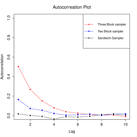
Figure 1: Autocorrelation plot of $\left({\bf Y}-X\bm{\beta}\right)^{T}\left({\bf Y}-X\bm{\beta}\right)+\sigma^{2}$ for simulated data with $n<p.$

Table 2: First ten autocorrelations for simulated data with $n>p$

Lag	1	2	3	4	5	6	7	8	9	10
Three block	0.5413	0.3497	0.2308	0.1562	0.1033	0.0638	0.0423	0.0231	0.0197	0.0143
Two Block	0.1155	0.0544	0.0297	0.0413	0.0340	0.0130	0.0043	-0.0022	0.0182	-0.0045
Sandwich	-0.0198	-0.0238	-0.0077	0.0512	-0.0079	0.0232	-0.0036	-0.0005	-0.0048	-0.0259

Figure 2: Autocorrelation plot of $\left({\bf Y}-X\bm{\beta}\right)^{T}\left({\bf Y}-X\bm{\beta}\right)+\sigma^{2}$ for simulated data with $n>p.$

6.2 Real data example

We consider the wheat data set from Perez and de los Campos [18], which is available in the R package BGLR. The data was obtained from numerous international trials across a wide variety of wheat-producing environments. For our analysis, we consider the average grain yield for a particular environmental condition (there are four to choose from) as the response variable, and 20 binary variables containing genotypic information as the predictors. We fit the Normal-Gamma model in (1) with $a=0.75,b=0.2,\xi=1,\alpha=0$ and compute autocorrelations for the function $\left({\bf Y}-X\bm{\beta}\right)^{T}\left({\bf Y}-X\bm{\beta}\right)+\sigma^{2}$ for the three block, two block and Haar PX-DA sandwich chains. The results are shown in Table 3 and Figure 3. As in the simulated data examples, the two-block chain has lower autocorrelations than the three-block chain, and the Haar PX-DA sandwich chain is the most efficient among all three Markov chains.

Table 3: First ten autocorrelations with wheat data

Lag	1	2	3	4	5	6	7	8	9	10
Three block	0.4579	0.2246	0.1193	0.0433	0.0214	0.0194	0.0166	0.0114	-0.0072	-0.0068
Two block	0.0799	0.0159	0.0053	0.0065	0.0072	0.0015	0.0022	-0.0224	-0.0103	-0.0131
Sandwich	0.0535	0.0163	0.0009	0.0344	0.0073	0.0308	-0.0190	-0.0438	-0.0098	-0.0161

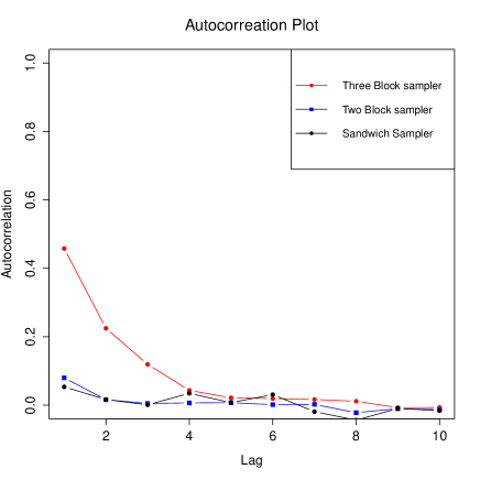
Figure 3: Autocorrelation plot of $\left({\bf Y}-X\bm{\beta}\right)^{T}\left({\bf Y}-X\bm{\beta}\right)+\sigma^{2}$ for the wheat data.

6.3 Discussion of numerical results

For both the simulated and real data settings, the two-block chain clearly has a significantly better performance than the three-block chain. For example, in all the settings the Lag 1 autocorrelation drops by 80% or more when we compare the three-block and the two-block chains. These findings support the theoretical results (Theorem 1 and Theorem 2) in the paper. Since the two-block chain and the three-block chain require the same computational effort, our theoretical and experimental results, support the overall conclusion that a practitioner should prefer the two-block chain over the three-block chain.

The comparison between the two-block and the Haar PX-DA chain is not as decisive. We elaborate on this below. Clearly, in all the experimental settings, the sandwich algorithm performs better than the two-block chain, and substantially so for the simulated datasets. These findings support the theoretical results (Lemma 5.1). However, note that the Haar PX-DA chain requires an extra computational step (sampling from $f_{\mathcal{G}}$) as compared to the two-block chain. This extra step requires a univariate rejection sampler. We have found that the performance of this rejection sampler varies with the choice of $a,b,\xi$ and $\alpha$. In the best case, it takes twice as much time as the other steps, and in the worst case, can take more than 10 times as much time as the other steps. Of course, the performance gains can sometimes easily offset this computational overhead, but a practitioner should make a careful determination in their specific setting.

Appendix

Proposition A 1.

Let $x\sim N(\mu,\sigma^{2}),$ then $\leavevmode\nobreak\ \int\limits_{0}^{c}\frac{1}{x}e^{-\frac{(x-\mu)^{2}}{2\sigma^{2}}}\,dx=\infty\leavevmode\nobreak\$ for any positive constant $c>0$.

Proof The result follows by noting that

$$x\cdot\left\lvert\frac{1}{x}e^{-\frac{(x-\mu)^{2}}{2\sigma^{2}}}\right\rvert\stackrel{{\scriptstyle\leavevmode\nobreak\ x\rightarrow 0^{+}}}{{\longrightarrow}}e^{-\frac{\mu^{2}}{2\sigma^{2}}}>0,$$

and $\int\limits_{0}^{c}\frac{1}{x}\,dx=\infty$. $\Box$

Proposition A 2.

Let $x\sim N(\mu,\sigma^{2}),$ then $\leavevmode\nobreak\ \int\limits_{0}^{c_{1}}\frac{1}{x(c_{2}-\ln x)}\leavevmode\nobreak\ e^{-\frac{(x-\mu)^{2}}{2\sigma^{2}}}\,dx=\infty\leavevmode\nobreak\$ for any positive constant $c_{1}$ and $c_{2}>\ln c_{1}$.

Proof We assume without loss of generality that $c_{1}<1$. The result follows by noting that

$$\frac{\frac{1}{x(c_{2}-\ln x)}\leavevmode\nobreak\ e^{-\frac{(x-\mu)^{2}}{2\sigma^{2}}}}{-\frac{1}{x\ln x}}=\frac{-\ln x}{c_{2}-\ln x}\leavevmode\nobreak\ e^{-\frac{(x-\mu)^{2}}{2\sigma^{2}}}\stackrel{{\scriptstyle\leavevmode\nobreak\ x\rightarrow 0^{+}}}{{\longrightarrow}}e^{-\frac{\mu^{2}}{2\sigma^{2}}}\in(0,\infty),$$

and

$$\leavevmode\nobreak\ \int\limits_{0}^{c_{1}}-\frac{1}{x\ln x}\,dx=\int\limits_{0}^{c_{1}}-\frac{1}{\ln x}\,d\ln x\leavevmode\nobreak\ \stackrel{{\scriptstyle t=\ln x}}{{=\joinrel=\joinrel=\joinrel=}}\int\limits_{-\infty}^{\ln c_{1}}-\frac{1}{t}\,dt=\int\limits_{-\ln c_{1}}^{\infty}\frac{1}{t}\,dt=\infty.$$

$\Box$

Proposition A 3.

Suppose the trandom variable U has a t-distribution with scale parameter $\kappa$ , location parameter $\vartheta$ and degrees of freedom $\nu.$ Then for $\nu>2,$

$$E(U^{2})\geq\frac{k^{2}\nu}{\nu-2}$$

.

Proof If the random variable $U$ has a t-distribution with scale parameter $\kappa,$ location parameter $\vartheta$ and degrees of freedom $\nu$ then $U=\vartheta+\kappa T$ where $T$ is a standard t-distribution with $\nu$ degrees of freedom. Hence

$$E(U^{2})=E(\vartheta+\kappa T)^{2} =E(\vartheta^{2}+\kappa^{2}T^{2}+2\vartheta\kappa T)$$

$$\geq E(\kappa^{2}T^{2}+2\vartheta\kappa T)$$

$$=\kappa^{2}E(T^{2})+2\vartheta\kappa E(T)$$

$$=\kappa^{2}(Var(T)+E^{2}(T))$$

$$=\frac{\kappa^{2}\nu}{\nu-2}.$$

$\Box$

Proposition A 4.

Let $\mu_{1}=e_{1}^{T}\mu,$ i.e. the first component of $\mu$, $\nu_{1}=2n+8p+4\alpha-1$, and $\epsilon_{1}=\sqrt{\frac{f_{2}(\bm{\beta},\tilde{\bm{\tau}})+1}{(2\lambda+\frac{1}{\tau_{1}}+\frac{1}{\tilde{\tau}_{1}})\nu_{1}}}$. Then there is a finite constant $f_{3}(\bm{\beta},\tilde{\bm{\tau}})$ such that

$$\int_{\mathbb{R}}\frac{\tilde{\beta}_{1}^{2}}{\left(1+\frac{\left(\tilde{\bm{\beta}}_{1}-\mu_{1}\right)^{2}}{\nu_{1}\epsilon_{1}^{2}}\right)^{\frac{1+\nu_{1}}{2}}}d{\tilde{{\beta}}_{1}}\geq f_{3}(\bm{\beta},\tilde{\bm{\tau}})\left(\frac{1}{2\lambda+\frac{1}{\tau_{1}}+\frac{1}{\tilde{\tau}_{1}}}\right)^{\frac{3}{2}}.$$

Proof Note that

$$\int_{\mathbb{R}}\frac{\tilde{\beta}_{1}^{2}}{\left(1+\frac{\left(\tilde{\bm{\beta}}_{1}-\mu_{1}\right)^{2}}{\nu_{1}\epsilon_{1}^{2}}\right)^{\frac{1+\nu_{1}}{2}}}d{\tilde{{\beta}}_{1}}=\epsilon_{1}\frac{\Gamma(\frac{\nu_{1}}{2})\sqrt{\pi\nu}}{\Gamma(\frac{\nu+1}{2})}E(U^{2}),$$

where $U$ follows a t-distribution with scale $\epsilon_{1},$ location $\mu_{1}$ and degrees of freedom $\nu_{1}.$ Using Proposition A3, we get that

$$\int_{\mathbb{R}}\frac{\tilde{\beta}_{1}^{2}}{\left(1+\frac{\left(\tilde{\bm{\beta}}_{1}-\mu_{1}\right)^{2}}{\nu_{1}\epsilon_{1}^{2}}\right)^{\frac{1+\nu_{1}}{2}}}d{\tilde{{\beta}}_{1}} =\epsilon_{1}\frac{\Gamma(\frac{\nu_{1}}{2})\sqrt{\pi\nu}}{\Gamma(\frac{\nu+1}{2})}E(U^{2})$$

$$\geq\frac{\Gamma(\frac{\nu_{1}}{2})\sqrt{\pi\nu}}{\Gamma(\frac{\nu+1}{2})}\frac{\nu_{1}}{\nu_{1}-2}\leavevmode\nobreak\ \epsilon_{1}^{3},$$

$$=\frac{\Gamma(\frac{\nu_{1}}{2})\sqrt{\pi\nu}}{\Gamma(\frac{\nu+1}{2})}\frac{\nu_{1}}{\nu_{1}-2}\left(\frac{f_{2}(\bm{\beta},\tilde{\bm{\tau}})+1}{\nu_{1}}\right)^{\frac{3}{2}}\left(\frac{1}{2\lambda+\frac{1}{\tau_{1}}+\frac{1}{\tilde{\tau}_{1}}}\right)^{\frac{3}{2}}$$

$$=f_{3}(\bm{\beta},\tilde{\bm{\tau}})\left({2\lambda+\frac{1}{\tau_{1}}+\frac{1}{\tilde{\tau}_{1}}}\right)^{-\frac{3}{2}}.$$

where $f_{3}(\bm{\beta},\tilde{\bm{\tau}})=\frac{\Gamma(\frac{\nu_{1}}{2})\sqrt{\pi\nu}}{\Gamma(\frac{\nu+1}{2})}\frac{\nu_{1}}{\nu_{1}-2}\left(\frac{f_{2}(\bm{\beta},\tilde{\bm{\tau}})+1}{\nu_{1}}\right)^{\frac{3}{2}}$. $\Box$