Two-dimensional Brownian random interlacements

Abstract

We introduce the model of two-dimensional continuous random interlacements, which is constructed using the Brownian trajectories conditioned on not hitting a fixed set (usually, a disk). This model yields the local picture of Wiener sausage on the torus around a late point. As such, it can be seen as a continuous analogue of discrete two-dimensional random interlacements [13]. At the same time, one can view it as (restricted) Brownian loops through infinity. We establish a number of results analogous to these of [12, 13], as well as the results specific to the continuous case.
Keywords: Brownian motion, conditioning, transience, Wiener moustache, logarithmic capacity, Gumbel process.
AMS 2010 subject classifications: Primary: 60J45; Secondary: 60G55, 60J65, 60K35.

${}^{~{}1}$Université Paris Diderot. Mathématiques, 8 place Aurélie Nemours, 75013 Paris, France.
Laboratoire de Probabilités, Statistique et Modélisation (LPSM), UMR 8001 CNRS-UPD-SU.
e-mail: comets@lpsm.paris

${}^{~{}2}$Department of Statistics, Institute of Mathematics, Statistics and Scientific Computation, University of Campinas – UNICAMP, rua Sérgio Buarque de Holanda 651, 13083–859, Campinas SP, Brazil
e-mail: popov@ime.unicamp.br

1 Introduction

The model of random interlacements in dimension $d\geq 3$ has been introduced in the discrete setting in [37] to describe the local picture of the trace left by the random walk on a large torus at a large time. It consists in a Poissonian soup of (doubly infinite) random walk paths modulo time-shift, which is a natural and general construction [27]. It has soon attracted the interest of the community, the whole field has now come to a maturity, as can be seen in two books [10, 19] dedicated to the model.

In the continuous setting and dimension $d\geq 3$, Brownian random interlacements bring the similar limit description for the Wiener sausage on the torus [29, 39]. Continuous setting is very appropriate to capture the geometrical properties of the sausage in their full complexity, see [20]. We also mention the “general” definition [35] of continuous RI, and an alternative definition of Brownian interlacements via Kuznetsov measures [16].

The model of two-dimensional (discrete) random interlacements was introduced in [13]. (For completeness, we mention here the one-dimensional case that has been studied in [7].) The point is that, in two dimensions, even a single trajectory of a simple random walk is space-filling, so the existence of the model has to be clarified together with its meaning. To define the process in a meaningful way on the planar lattice, one uses the SRW’s trajectories conditioned on never hitting the origin, and it gives the local limit of the trace of the walk on a large torus at a large time given that the origin has not been visited so far. We mention also the recent alternative definition [34] of the two-dimensional random interlacements in the spirit of thermodynamic limit. A sequence of finite volume approximation is introduced, consisting in random walks killed with intensity depending on the spatial scale and restricted to paths avoiding the origin. Two versions are presented, using Dirichlet boundary conditions outside a box or by killing the walk at an independent exponential random time.

The interlacement gives the structure of late points and accounts for their clustering studied in [15]. They convey information on the cover time, for which the LLN was obtained in [14]. Let us mention recent results for the cover time in two dimensions in the continuous case: (i) computation of the second order correction to the typical cover time on the torus [4], (ii) tightness of the cover time relative to its median for Wiener sausage on the Riemann sphere [5].

In this paper we define the two-dimensional Brownian random interlacements, implementing the program of [13] in the continuous setting; similarly to the discrete case, they are made of conditioned (on not hitting the unit disk) Brownian paths. Again, similarly to the discrete case, it holds that the Brownian random interlacements arise as a limit of the picture seen from a fixed point on the torus, given that this point remains uncovered by the Brownian sausage. In fact, we find that the purity of the concepts and the geometrical interest of the interlacement and of its vacant set are uncomparably stronger here. From a different perspective, we also obtain fine properties of Brownian loops through infinity which shows that the two models are equivalent by inversion in the complex plane.

For our purpose, we introduce the Wiener moustache, which is the doubly infinite path used in the soup. The Wiener moustache is obtained by pasting two independent Brownian motions conditioned to stay outside the unit disk starting from a random point on the circle. The conditioned Brownian motion is itself an interesting object, it seems to be overlooked in spite of the extensive literature on the planar Brownian motion, cf. [26]. It is defined as a Doob’s $h$-transform, see Chapter X of Doob’s book [17] about conditional Brownian motions; see also [18] for an earlier approach via transition semigroup. A modern exposition of methods and difficulties in conditioning a process by a negligible set is [36]. For a perspective from non equilibrium physics, see [9, Section 4].

We also study the process of distances of a point to the BRI as the level increases. After a non-linear transformation in time and space, the process has a large-density limit given by a pure jump process with a drift. The limit is stationary with the negative of a Gumbel distribution for invariant measure, and it is in fact related to models for congestion control on Internet (TCP/IP), see [2, 3].

2 Formal definitions and results

In Section 2.1 we discuss the Brownian motion conditioned on never returning to the unit disk (this is the analogue of the walk ${\widehat{S}}$ in the discrete case, cf. [12, 13]), and define an object called Wiener moustache, which will be the main ingredient for constructing the Brownian random interlacements in two dimensions. In Section 2.2 we formally define the Brownian interlacements, and in Section 2.3 we state our main results.

In the following, we will identify ${\mathbb{R}}^{2}$ and ${\mathbb{C}}$ via $x=(x_{1},x_{2})=x_{1}+ix_{2}$, $\|\cdot\|$ will denote the Euclidean norm in ${\mathbb{R}}^{2}$ or ${\mathbb{Z}}^{2}$ as well as the modulus in ${\mathbb{C}}$, and let ${\mathsf{B}}(x,r)=\{y:\|x-y\|\leq r\}$ be the (closed) disk of radius $r$ centered in $x$, and abbreviate ${\mathsf{B}}(r):={\mathsf{B}}(0,r)$.

2.1 Brownian motion conditioned on staying outside a disk, and Wiener moustache

Let $W$ be a standard two-dimensional Brownian motion. For $A\subset{\mathbb{R}}^{2}$ define the stopping time

$$\tau(A)=\inf\{t>0:W_{t}\in A\},$$ (2.1)

and let us use the shorthand $\tau(r):=\tau\big{(}\partial{\mathsf{B}}(r)\big{)}$. It is well known that $h(x)=\ln\|x\|$ is a fundamental solution of Laplace equation,

$${}\frac{1}{2}\Delta h=\pi\delta_{0},$$

with $\delta_{0}$ being the Dirac mass at the origin and $\Delta={\partial_{x_{1}}^{2}}+{\partial_{x_{2}}^{2}}$ the Laplacian.

An easy consequence of $h$ being harmonic away from the origin and of the optional stopping theorem is that, for any $0<a<\|x\|<b<\infty$,

$${\mathbb{P}}_{x}[\tau(b)<\tau(a)]=\frac{\ln(\|x\|/a)}{\ln(b/a)}\;.$$ (2.2)

Since $h$ is non-negative outside the ball ${\mathsf{B}}(1)$ and vanishes on the boundary, a further consequence of harmonicity is that, under ${\mathbb{P}}_{x}$ for $\|x\|>1$,

$${}{\mathbf{1}}_{\{t<\tau(1)\}}\frac{h(W_{t})}{h(x)}\equiv\frac{h(W_{t\wedge\tau(1)})}{h(x)}$$

is a non-negative martingale with mean 1. Thus, the formula

$${\mathbb{P}}_{x}\big{[}\widehat{W}\in A\big{]}={\mathbb{E}}_{x}\Big{(}{\mathbf{1}}_{\{W\in A\}}{\mathbf{1}}_{\{t<\tau(1)\}}\frac{h(W_{t})}{h(x)}\Big{)}\;,$$ (2.3)

for all $t>0$, for $A\in{\cal F}_{t}$ ($\sigma$-field generated by the evaluation maps at times $\leq t$ in ${\cal C}({\mathbb{R}}_{+},{\mathbb{R}}^{2})$), defines a continuous process $\widehat{W}$ on $[0,{\infty})$ starting at $x$ and taking values in ${\mathbb{R}}^{2}\setminus{\mathsf{B}}(1)$.

The process defined as the Doob’s $h$-transform of the standard Brownian motion by the function $h(x)=\ln\|x\|$, can be seen as the Brownian motion conditioned on never hitting ${\mathsf{B}}(1)$, as it appears in Lemma 2.1 below. Similarly to (2.1), we define

$$\widehat{\tau}(A)=\inf\big{\{}t>0:\widehat{W}_{t}\in A\big{\}}$$ (2.4)

and use the shorthand $\widehat{\tau}(r):=\widehat{\tau}\big{(}\partial{\mathsf{B}}(r)\big{)}$. For a ${\mathbb{R}}^{2}$-valued process $X=(X_{t},t\geq 0)$ we will distinguish its geometric range $X_{{\mathcal{I}}}$ on some time interval ${\mathcal{I}}$ from its restriction $X_{\big{|}{\mathcal{I}}}$,

$$X_{{\mathcal{I}}}=\bigcup_{t\in{\mathcal{I}}}\{X_{t}\}\;,\qquad X_{\big{|}{\mathcal{I}}}:t\in{\mathcal{I}}\mapsto X_{t}\;.$$ (2.5)

Lemma 2.1.

For all $R>1$ and all $x\in{\mathbb{R}}^{2}$ such that $1<\|x\|<R$ we have

$${\mathbb{P}}_{x}\Big{[}W_{\big{|}[0,\tau(R)]}\in\cdot\mid\tau(R)<\tau(1)\Big{]}={\mathbb{P}}_{x}\Big{[}\widehat{W}_{\big{|}[0,\widehat{\tau}(R)]}\in\cdot\,\Big{]}.$$ (2.6)

Proof.

From (2.3) it follows that for $A\in{\cal F}_{\tau(R)}$,

$${\mathbb{P}}_{x}\big{[}\widehat{W}\in A\big{]} ={\mathbb{E}}_{x}\Big{(}{\mathbf{1}}_{\{W\in A\}}{\mathbf{1}}_{\{\tau(R)<\tau(1)\}}\frac{h(W_{\tau(R)})}{h(x)}\Big{)}$$

$$={\mathbb{E}}_{x}\Big{(}{\mathbf{1}}_{\{W\in A\}}{\mathbf{1}}_{\{\tau(R)<\tau(1)\}}\Big{)}\frac{h(R)}{h(x)}\;,$$

which is the desired equality in view of (2.2). ∎

From (2.3) we derive the transition kernel of $\widehat{W}$: for $\|x\|>1,\|y\|\geq 1$,

$${\hat{p}}(t,x,y)=p_{0}(t,x,y)\frac{\ln\|y\|}{\ln\|x\|}.$$ (2.7)

where $p_{0}$ denotes the transition subprobability density of $W$ killed on hitting the unit disk ${\mathsf{B}}(1)$. Thus, the semigroup $\mathchoice{\accentset{\displaystyle\text{\smash{\raisebox{-5.59721pt}{$\widehatsym$}}}}{P}}{\accentset{\textstyle\text{\smash{\raisebox{-5.59721pt}{$\widehatsym$}}}}{P}}{\accentset{\scriptstyle\text{\smash{\raisebox{-3.91806pt}{$\widehatsym$}}}}{P}}{\accentset{\scriptscriptstyle\text{\smash{\raisebox{-2.7986pt}{$\widehatsym$}}}}{P}}_{t}$ of the process $\widehat{W}$ is given by

$$\mathchoice{\accentset{\displaystyle\text{\smash{\raisebox{-5.59721pt}{$\widehatsym$}}}}{P}}{\accentset{\textstyle\text{\smash{\raisebox{-5.59721pt}{$\widehatsym$}}}}{P}}{\accentset{\scriptstyle\text{\smash{\raisebox{-3.91806pt}{$\widehatsym$}}}}{P}}{\accentset{\scriptscriptstyle\text{\smash{\raisebox{-2.7986pt}{$\widehatsym$}}}}{P}}_{t}f(x)=h(x)^{-1}P^{0}_{t}\big{(}hf\big{)}(x),$$

for bounded functions $f$ vanishing on ${\mathsf{B}}(1)$, where $P^{0}_{t}=e^{(t/2)\Delta_{0}}$ with $\Delta_{0}$ being the Laplacian with Dirichlet boundary conditions on ${\mathbb{R}}^{2}\setminus{\mathsf{B}}(1)$. From the above formula we compute its generator,

$${}\mathchoice{\accentset{\displaystyle\text{\smash{\raisebox{-5.59721pt}{$\widehatsym$}}}}{L}}{\accentset{\textstyle\text{\smash{\raisebox{-5.59721pt}{$\widehatsym$}}}}{L}}{\accentset{\scriptstyle\text{\smash{\raisebox{-3.91806pt}{$\widehatsym$}}}}{L}}{\accentset{\scriptscriptstyle\text{\smash{\raisebox{-2.7986pt}{$\widehatsym$}}}}{L}}f(x) =\lim_{t\searrow 0}t^{-1}\big{[}\mathchoice{\accentset{\displaystyle\text{\smash{\raisebox{-5.59721pt}{$\widehatsym$}}}}{P}}{\accentset{\textstyle\text{\smash{\raisebox{-5.59721pt}{$\widehatsym$}}}}{P}}{\accentset{\scriptstyle\text{\smash{\raisebox{-3.91806pt}{$\widehatsym$}}}}{P}}{\accentset{\scriptscriptstyle\text{\smash{\raisebox{-2.7986pt}{$\widehatsym$}}}}{P}}_{t}f(x)-f(x)\big{]}$$

$$=h(x)^{-1}\lim_{t\searrow 0}t^{-1}\big{[}P^{0}_{t}(hf)(x)-(hf)(x)\big{]}$$

$$=\frac{1}{2h(x)}\Delta\big{(}hf\big{)}(x)$$ (2.8)

$$=\frac{1}{2}\Delta f+\frac{x}{\|x\|^{2}\ln\|x\|}\cdot\nabla f,$$ (2.9)

using $\Delta_{0}(hf)=\Delta(hf)$ and harmonicity of $h$. Thus the diffusion $\widehat{W}$ obeys the stochastic differential equation

$$d\widehat{W}_{t}=\frac{\widehat{W}_{t}}{\|\widehat{W}_{t}\|^{2}\ln\|\widehat{W}_{t}\|}dt+dW_{t}.$$ (2.10)

Sometimes it will be useful to consider an alternative definition of the diffusion $\widehat{W}$ using polar coordinates, $\widehat{W}_{t}=({\mathcal{R}}_{t}\cos\Theta_{t},{\mathcal{R}}_{t}\sin\Theta_{t})$. With $W^{(1,2)}$ two independent standard linear Brownian motions, consider the stochastic differential equations

$$d{\mathcal{R}}_{t} =\Big{(}\frac{1}{{\mathcal{R}}_{t}\ln{\mathcal{R}}_{t}}+\frac{1}{2{\mathcal{R}}_{t}}\Big{)}dt+dW_{t}^{(1)},$$ (2.11)

and

$$d\Theta_{t} =\frac{1}{{\mathcal{R}}_{t}}dW_{t}^{(2)}$$ (2.12)

where the diffusion $\Theta$ takes values on the whole ${\mathbb{R}}$; it is an easy exercise in stochastic calculus to show that (2.10) is equivalent to (2.11)–(2.12).

Since the norm of the 2-dimensional Brownian motion $W$ is a BES² process and $\widehat{W}$ is $W$ conditioned to have norm larger than $1$ (recall Lemma 2.1), the process ${\mathcal{R}}=\|\widehat{W}\|$ is itself a BES² conditioned on being in $(1,{\infty})$. For further use, we give an alternative proof of this fact. The BES² process has generator and scale function given by

$$L_{{\rm BES}^{2}}f(r)=\frac{1}{2r}\big{(}rf^{\prime}(r)\big{)}^{\prime}\;,\qquad s(r)=\ln r.$$ (2.13)

Following Doob [18], the infinitesimal generator of BES² conditioned on being in $[1,{\infty})$ is

$$[s\!-\!s(1)]^{-1}L_{{\rm BES}^{2}}\big{(}[s\!-\!s(1)]f\big{)}=\frac{1}{2}\Big{(}f^{\prime\prime}+\Big{(}\frac{1}{r\ln r}+\frac{1}{2r}\Big{)}f^{\prime}\Big{)},$$ (2.14)

which coincides with the one of the process ${\mathcal{R}}$.

It is elementary to obtain from (2.11) that

$${}d\frac{1}{\ln{\mathcal{R}}_{t}}=\frac{-1}{{\mathcal{R}}_{t}\ln^{2}{\mathcal{R}}_{t}}dW_{t}^{(1)},$$

so $(\ln{\mathcal{R}}_{t})^{-1}=\big{(}\ln\|\widehat{W}_{t}\|\big{)}^{-1}$ is a local martingale. (Alternatively, this can be seen directly from (2.7).)

We will need to consider the process $\widehat{W}$ starting from $\widehat{W}_{0}=w$ with unit norm. Since the definition (2.10) makes sense only when starting from $w,\|w\|>1$, we now extend it to the case when $\|w\|=1$. Consider $X$ a 3-dimensional Bessel process BES${}^{3}(x)$, i.e., the norm of a 3-dimensional Brownian motion starting form a point of norm $x$. It solves the SDE

$${}dX_{t}=\frac{1}{X_{t}}dt+dB_{t},\qquad X_{0}=x\geq 0,$$

with $B$ a 1-dimensional Brownian motion on some probability space $(\Omega,{\mathcal{A}},P)$. Denoting by ${\mathcal{F}}_{t}$ the $\sigma$-field generated by $B$ up to time $t$, we consider the probability measure $Q$ on ${\mathcal{F}}_{\infty}$ given by ${\frac{dQ}{dP}}\big{|}_{{\mathcal{F}}_{t}}=Z_{t},t\geq 0$, where

$$Z_{t}=\exp\Big{(}\int_{0}^{t}\varphi(X_{s})dB_{s}-\frac{1}{2}\int_{0}^{t}\varphi(X_{s})^{2}ds\Big{)},$$ (2.15)

with

$${}\varphi(x)=\begin{cases}\displaystyle\frac{1}{2(1+x)}+\displaystyle\frac{1}{(1+x)\ln(1+x)}-\displaystyle\frac{1}{x},&\text{ if }x>0,\\ 1/2,\phantom{\int\limits_{a}^{B}}&\text{ if }x=0.\end{cases}$$

Then, $\varphi(X_{t})$ is progressively measurable and bounded, so $Z_{t}$ is a $P$-martingale. By Girsanov theorem, we see that

$$\tilde{B}_{t}=B_{t}-\int_{0}^{t}\varphi(X_{s})\,ds$$

is a Brownian motion under $Q$. Now, the integral formula

$${}X_{t}=X_{0}+\int_{0}^{t}\left(\frac{1}{2(1+X_{s})}+\frac{1}{(1+X_{s})\ln(1+X_{s})}\right)ds+{\tilde{B}}_{t},\qquad t\geq 0,$$

and uniqueness of the solution of the above SDE show that the law of $1+X$ under $Q$ is the law of ${\mathcal{R}}$ under $P$, provided that $X_{0}>0$.

Definition 2.2.

We define the process ${\mathcal{R}}$ starting from ${\mathcal{R}}_{0}=1$ in the following way: it has the same law as $1+X$ under $Q$ with $X_{0}=0$. Similarly, we define the law of the process $\widehat{W}$ starting from $w\in{\mathbb{R}}^{2}$ with unit norm as the law of $({\mathcal{R}}_{t},\Theta_{t})_{t}$ with ${\mathcal{R}}$ as above and $\Theta$ given by its law conditional on ${\mathcal{R}}$ as in (2.12).

Then, the process ${\mathcal{R}}$ (respectively, $\widehat{W}$) is the limit as $\varepsilon\to 0$ of processes started from $1+\varepsilon$ (respectively, from $(1+\varepsilon)w$). This follows from the identities

$${}{\mathbb{E}}f({\mathcal{R}}_{t})=E^{Q}f(1+X_{t})=E^{P}\big{[}Z_{t}f(1+X_{t})\big{]},$$

with $Z_{t}$ from (2.15) and $X$ depending continuously on its initial condition $X_{0}\geq 0$.

Let us mention some elementary but useful reversibility and scaling properties of $\widehat{W}$.

Proposition 2.3.

• The diffusion $\widehat{W}$ is reversible for the measure with density $\ln^{2}\|x\|$ with respect to the Lebesgue measure on ${\mathbb{R}}^{2}\setminus{\mathsf{B}}(1)$.

• The diffusion ${\mathcal{R}}$ is reversible for the measure $r\ln^{2}r\,dr$ on $(1,{\infty})$.

• Let $1\leq a\leq\|x\|$. Then, the law of $\widehat{W}$ starting from $x$ conditioned on never hitting ${\mathsf{B}}(a)$ is equal to the law of the process $(a\widehat{W}(ta^{-2});t\geq 0)$ with $\widehat{W}$ starting from $x/a$.

• For $1\leq a\leq r$, the law of ${\mathcal{R}}$ starting from $r$ conditioned on staying strictly greater than $a$ is equal to that of $(a{\mathcal{R}}(a^{-2}t))_{t\geq 0}$ with ${\mathcal{R}}_{0}=r/a$.

Proof.

For smooth $f,g:{\mathbb{R}}^{2}\setminus{\mathsf{B}}(1)\to{\mathbb{R}}$, we have

$$\hat{\varepsilon}(f,g):=-\int_{{\mathbb{R}}^{2}\setminus{\mathsf{B}}(1)}f(x)\mathchoice{\accentset{\displaystyle\text{\smash{\raisebox{-5.59721pt}{$\widehatsym$}}}}{L}}{\accentset{\textstyle\text{\smash{\raisebox{-5.59721pt}{$\widehatsym$}}}}{L}}{\accentset{\scriptstyle\text{\smash{\raisebox{-3.91806pt}{$\widehatsym$}}}}{L}}{\accentset{\scriptscriptstyle\text{\smash{\raisebox{-2.7986pt}{$\widehatsym$}}}}{L}}g(x)h^{2}(x)\,dx\stackrel{{\scriptstyle}}{{=}}\frac{1}{2}\int_{{\mathbb{R}}^{2}\setminus{\mathsf{B}}(1)}{\nabla(hf)}\cdot\nabla(hg)\,dx,$$

by (2.8) and integration by parts. Since this is a symmetric function of $f,g$, claim (i) follows. For (ii), using (2.11), we write the generator of ${\mathcal{R}}$ as

$${}L_{{\mathcal{R}}}f(r)=\frac{1}{2r\ln^{2}r}\big{(}f^{\prime}(r)r\ln^{2}r\big{)}^{\prime},$$

for smooth $f:(1,{\infty})\to{\mathbb{R}}$, and conclude by a similar computation.

For a Brownian motion $W$ starting from $x/a$, the scaled process $W^{(a)}(t)=aW(t/a^{2})$ is a Brownian motion starting from $x$. Since $\widehat{W}$ is the Brownian motion conditioned on never hitting ${\mathsf{B}}(1)$, the process $(a\widehat{W}(ta^{-2});t\geq 0)$ has the law of $W$ conditioned on never hitting ${\mathsf{B}}(a)$. In turn, the latter has the same law as $\widehat{W}$ starting from $x$ conditioned on never hitting ${\mathsf{B}}(a)$. We have proved (iii). Claim (iv) follows directly from (iii) and the definition of ${\mathcal{R}}$ as the norm of $\widehat{W}$. ∎

Since $\big{(}\!\ln\|\widehat{W}_{t}\|\big{)}^{-1}$ is a local martingale, the optional stopping theorem implies that for any $1<a<\|x\|<b<\infty$

$${\mathbb{P}}_{x}[\widehat{\tau}(b)<\widehat{\tau}(a)]=\frac{(\ln a)^{-1}-(\ln\|x\|)^{-1}}{(\ln a)^{-1}-(\ln b)^{-1}}=\frac{\ln(\|x\|/a)\times\ln b}{\ln(b/a)\times\ln\|x\|}.$$ (2.16)

Sending $b$ to infinity in (2.16) we also see that for $1\leq a\leq\|x\|$

$${\mathbb{P}}_{x}[\widehat{\tau}(a)=\infty]=1-\frac{\ln a}{\ln\|x\|}.$$ (2.17)

Now, we introduce one of the main objects of this paper:

Definition 2.4.

Let $U$ be a random variable with uniform distribution on $[0,2\pi]$, and let $({\mathcal{R}}^{(1,2)},\Theta^{(1,2)})$ be two independent copies of the two-dimensional diffusion on ${\mathbb{R}}_{+}\times{\mathbb{R}}$ defined by (2.11)–(2.12), with common initial point $(1,U)$. Then, the Wiener moustache $\eta$ is defined as the union of ranges of the two trajectories, i.e.,

$$\eta=\big{\{}(r,\theta):\text{ there exist }k\in\{1,2\},t\geq 0\text{ such that }{\mathcal{R}}^{(k)}_{t}=r,\Theta^{(k)}_{t}=\theta\big{\}}.$$

When there is no risk of confusion, we also call the Wiener moustache the image of the above object under the map $(r,\theta)\mapsto(r\cos\theta,r\sin\theta)$ (see below).

We stress that we view the trajectory of a process as a geometric subset of ${\mathbb{R}}^{2}$, forgetting its time parametrization.

Informally, the Wiener moustache is just the union of two independent Brownian trajectories started from a random point on the boundary of the unit disk, conditioned on never re-entering this disk, see Figure 1.

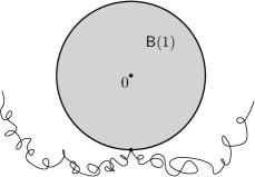
Figure 1: An instance of Wiener moustache (for aestetical reasons, the starting point was randomly chosen to be $x=(0,-1)$).

One can also represent the Wiener moustache as one doubly-infinite trajectory $(\widehat{W}_{t},t\in{\mathbb{R}})$, where $\|\widehat{W}_{0}\|=1$, $\|\widehat{W}_{t}\|>1$ for all $t\neq 0$.

Remark 2.5.

The Brownian motion $\widehat{W}^{b}$ conditioned not to enter in the ball ${\mathsf{B}}(b)$ of radius $b>0$ can be defined similarly to above. Proposition 2.3 (iii) and Lemma 2.1 imply that, in law,

$$\widehat{W}^{b}(t)=b\widehat{W}(b^{-2}t)\;,\quad t\geq 0.$$

Therefore, the set of visited points and the connected component of $0$ in its complement are simply the $b$-homothetics of the Wiener moustache.

2.2 Two-dimensional Brownian random interlacements

Now, we are able to define the model of Brownian random interlacements in the plane. We prefer not to imitate the corresponding construction of [13] of discrete random interlacements which uses a general construction of [40] of random interlacements on transient weighted graphs; instead of defining a consistent family of probability measures on closed subsets of bounded regions, we rather give an “infinite volume description” of the model.

Definition 2.6.

Let $\alpha>0$ and consider a Poisson point process $(\rho_{k}^{\alpha},k\in{\mathbb{Z}})$ on ${\mathbb{R}}_{+}$ with intensity $r(\rho)=\frac{2\alpha}{\rho},\rho\in{\mathbb{R}}_{+}$. Let $(\eta_{k},k\in{\mathbb{Z}})$ be an independent sequence of i.i.d. Wiener moustaches. Fix also $b\geq 0$. Then, the model of Brownian Random Interlacements (BRI) on level $\alpha$ truncated at $b$ is defined as the following subset of ${\mathbb{R}}^{d}\setminus{\mathsf{B}}(1)$ (see Figure 2):

$$\mathop{\mathrm{BRI}}(\alpha;b)=\bigcup_{k:\rho_{k}^{\alpha}\geq b}\rho_{k}^{\alpha}\eta_{k}\,.$$ (2.18)

Let us abbreviate $\mathop{\mathrm{BRI}}(\alpha):=\mathop{\mathrm{BRI}}(\alpha;1)$. As shown on Figure 2 on the left, the Poisson process with rate $r(\rho)=\frac{2\alpha}{\rho}$ can be obtained from a two-dimensional Poisson point process with rate $1$ in the first quadrant, by projecting onto the horizontal axis those points which lie below $r(\rho)$. Since the area under $r(\rho)$ is infinite in the neighborhoods of $0$ and $\infty$, there is a.s. an infinite number of points of the Poisson process in both $(0,\varepsilon)$ and $(M,\infty)$ for all positive $\varepsilon$ and $M$.

An important observation is that the above Poisson process is the image of a homogeneous Poisson process of rate $1$ in ${\mathbb{R}}$ under the map $x\mapsto e^{x/2\alpha}$ (or, equivalently, the image of a homogeneous Poisson process of rate $2\alpha$ under the map $x\mapsto e^{x}$); this is a straightforward consequence of the Mapping Theorem for Poisson processes (see e.g. Section 2.3 of [22]). In particular, we may write

$$\rho_{k}^{\alpha}=\exp\Big{(}\frac{Y_{1}+\cdots+Y_{k}}{2\alpha}\Big{)},$$ (2.19)

where $Y_{1},\ldots,Y_{k}$ are i.i.d. Exponential(1) random variables.

Remark 2.7.

From the above, it follows that we can construct $\mathop{\mathrm{BRI}}(\alpha;0)$ – and hence also $\mathop{\mathrm{BRI}}(\alpha;b)$ for all $b>0$ – simultaneously for all $\alpha>0$ in the following way (as shown on the left side of Figure 2): consider a two-dimensional Poisson point process of rate $1$ in ${\mathbb{R}}^{2}_{+}$, and then take the abscissa of the points below the graph of $r(\rho)=\frac{2\alpha}{\rho}$ to be the distances to the origin of the corresponding Wiener’s moustaches. In view of the previous observation, an equivalent way to do this is to consider a Poisson point process of rate $1$ in ${\mathbb{R}}\times{\mathbb{R}}_{+}$, take the first coordinates of points with second coordinate at most $2\alpha$, and exponentiate.

Observe also that, by construction, for all positive $\alpha,\beta,b$ it holds that

$$\mathop{\mathrm{BRI}}(\alpha;b)\oplus\mathop{\mathrm{BRI}}(\beta;b)\stackrel{{\scriptstyle\text{\tiny law}}}{{=}}\mathop{\mathrm{BRI}}(\alpha+\beta;b),$$ (2.20)

where $\oplus$ means superposition of independent copies.

Figure 2: On the definition of $\mathop{\mathrm{BRI}}(\alpha;b)$

At this point it is worth mentioning that the (discrete) random interlacements may be regarded as Markovian loops “passing through infinity”, see e.g. Section 4.5 of [38]. In the continuous case, we note that the object we just constructed can be viewed as “Brownian loops through infinity”. More precisely, we have a simple relation to the Brownian loop measure defined in [25] (see also [24]) and studied in [43]:

Theorem 2.8.

Consider a Poisson process of loops rooted in the origin with the intensity measure $2\pi\alpha\mu(0,0)$, with $\mu(\cdot,\cdot)$ as defined in Section 3.1.1 of [25]. Then, the inversion (i.e., the image under the map $z\mapsto 1/z$) of this family of loops is $\mathop{\mathrm{BRI}}(\alpha;0)$. The inversion of the loop process restricted on ${\mathsf{B}}(1)$ is $\mathop{\mathrm{BRI}}(\alpha)$.

Proof.

This readily follows from Theorem 1 of [31] and the invariance of Brownian trajectories under conformal mappings. ∎

Remark 2.9.

Analogously to (2.7)–(2.9) one can also define a diffusion $\widehat{W}^{(L)}$ avoiding a compact set $L\subset{\mathbb{C}}$ such that ${\mathbb{C}}\setminus L$ is simply connected on the Riemann sphere. Observe that, by the Riemann mapping theorem, there exists a unique conformal map $\varphi$ that sends the exterior of ${\mathsf{B}}(1)$ to the exterior of $L$ and also satisfies the conditions $\varphi(\infty)=\infty$, $\varphi^{\prime}(\infty)>0$. We then define $\mathop{\mathrm{BRI}}(\alpha;L)$ as $\varphi(\mathop{\mathrm{BRI}}(\alpha))$, see Figure 3.

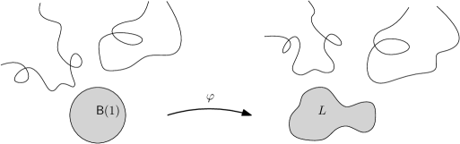
Figure 3: On the definition of random interlacements avoiding the domain $L$

Next, we need also to introduce the notion of capacity in the plane. Let $A$ be a compact subset of ${\mathbb{R}}^{2}$ such that ${\mathsf{B}}(1)\subset A$. Let $\mathop{\mathrm{hm}}\nolimits_{A}$ be the harmonic measure (from infinity) on $A$, that is, the entrance law in $A$ for the Brownian motion starting from infinity, cf. e.g. Theorem 3.46 of [30]. We define the capacity of $A$ as

$$\mathop{\mathrm{cap}}(A)=\frac{2}{\pi}\int_{A}\ln\|y\|\,d\mathop{\mathrm{hm}}\nolimits_{A}(y).$$ (2.21)

We stress that there exist other definitions of capacity; a common one, called the logarithmic capacity in Chapter 5 of [33], is given by the exponential of (2.21) without the constant $\frac{2}{\pi}$ in front. However, in this paper, we prefer the above definition (2.21) which matches the corresponding “discrete” capacity for random walks, cf. e.g. Chapter 6 of [23]. Note that (2.21) immediately implies that $\mathop{\mathrm{cap}}(A)\geq 0$ for $A\supset{\mathsf{B}}(1)$, and

$$\mathop{\mathrm{cap}}\!\big{(}{\mathsf{B}}(r)\big{)}=\frac{2}{\pi}\ln r$$ (2.22)

for any radius $r$. Next, we need to define the harmonic measure $\mathop{\widehat{\mathrm{hm}}}\nolimits_{A}$ for the (transient) conditioned diffusion $\widehat{W}$. For a compact, non polar set $A\subset{\mathbb{R}}^{2}$ (see, e.g.  [30, p.234]), with $A\subset{\mathbb{R}}^{2}\setminus\mathring{{\mathsf{B}}}(1)$ and $M\subset\partial A$, let

$${}\mathop{\widehat{\mathrm{hm}}}\nolimits_{A}(M)=\lim_{\|x\|\to\infty}{\mathbb{P}}_{x}\big{[}\widehat{W}_{\widehat{\tau}(A)}\in M\mid\widehat{\tau}(A)<\infty\big{]},$$

where the existence of the limit follows e.g. from Lemma 3.10 below. Observe that for any $A$ as above it holds that $\mathop{\widehat{\mathrm{hm}}}\nolimits_{A}\big{(}{\mathsf{B}}(1)\cap\partial A\big{)}=0$.

Now, we show that we have indeed defined the “right” object in (2.18):

Proposition 2.10.

• for any compact $A\subset{\mathbb{R}}^{2}$ such that ${\mathsf{B}}(1)\subset A$, we have

  $${\mathbb{P}}\big{[}A\cap\mathop{\mathrm{BRI}}(\alpha)=\emptyset\big{]}=\exp\big{(}-\pi\alpha\mathop{\mathrm{cap}}(A)\big{)}.$$ (2.23)

  Equivalently, for $A$ compact, ${\mathbb{P}}\big{[}A\cap\mathop{\mathrm{BRI}}(\alpha)=\emptyset\big{]}=\exp\big{(}-\pi\alpha\mathop{\mathrm{cap}}(A\cup{\mathsf{B}}(1))\big{)}.$

• the trace of $\mathop{\mathrm{BRI}}(\alpha)$ on any compact set $A$ such that ${\mathsf{B}}(1)\subset A$ can be obtained using the following procedure:

  • take a Poisson($\pi\alpha\mathop{\mathrm{cap}}(A)$) number of particles;

  • place these particles on the boundary of $A$ independently, with distribution $\mathop{\widehat{\mathrm{hm}}}\nolimits_{A}$;

  • let the particles do independent $\widehat{W}$-diffusions (since $\widehat{W}$ is transient, each walk only leaves a nowhere dense trace on $A$).

We postpone the proof of this result to Section 4. Let us stress that (2.23) is the characteristic property of random interlacements, compare to (2) of [13]. As explained just after Definition 2.1 of [13], the factor $\pi$ is there just for convenience, since it makes the formulas cleaner. Also, the construction in (ii) of $\mathop{\mathrm{BRI}}(\alpha)$ on $A$ agrees with the corresponding discrete “constructive description” of [13], and is presented in larger details just after Definition 2.1 there.

Next, for a generic function $g:{\mathbb{C}}\mapsto{\mathbb{C}}$, we denote by $g\big{(}\!\mathop{\mathrm{BRI}}(\alpha;b)\big{)}$ the image of $\mathop{\mathrm{BRI}}(\alpha;b)$ under the map $g$. We will also need from $g$ that the image of a Wiener moustache is itself a Wiener moustache. Thus, one needs to give a special treatment to power functions of the form $g(z)=z^{\lambda}$ for a noninteger $\lambda$. We will use the polar representation, so that the complex-valued power function now has a natural definition,

$$\text{for }r>0\text{ and }\theta\in{\mathbb{R}},\quad(r,\theta)^{\lambda}:=(r^{\lambda},\lambda\theta);$$ (2.24)

for arbitrary $\lambda>0$. However this transformation does not preserve the law of Wiener moustache. Indeed, the angular coordinates of the initial points of the moustaches to be uniform in the interval $[0,2\pi)$. If we then apply the power map with, say, $\lambda=1/2$, then all the initial points will have their angular coordinates in $[0,\pi)$, breaking the isotropy.

In this concrete case this can be repaired by choosing the angular coordinates of the initial points in the interval $[0,4\pi)$, but what to do for other (possibly irrational) values of $\lambda$?

Here, we present a construction that works for all $\lambda>0$ simultaneously, but uses an additional sequence $\xi=(\xi_{1},\xi_{2},\xi_{3},\ldots)$ of i.i.d. Uniform$[0,2\pi)$ random variables. Let $\Theta_{k}$ be the angular coordinate of the initial point of $\eta_{k}$, the $k$th moustache. For all $\lambda>0$, set

$$\Theta_{k}^{(\lambda)} =\lambda(\Theta_{k}-\xi_{k})+\xi_{k}\mod 2\pi$$

$$=\lambda\Theta_{k}+(1-\lambda)\xi_{k}\mod 2\pi;$$

observe that $\Theta_{k}^{(\lambda)}$ is also Uniform$[0,2\pi)$. Also, $\Theta_{k}\mapsto\Theta_{k}^{(\lambda)}$ seen as a function on ${\mathbb{R}}/2\pi{\mathbb{Z}}$ varies continuously in $\lambda$. The extra randomization carried by the sequence $\xi_{k}$ defines a transformation on the law of $\mathop{\mathrm{BRI}}(\alpha;b)$, where the scaling of the angle is performed with respect to a reference angle $\xi_{k}$: if $(r,\theta)$ belongs to the $k$-th moustache, its image by the power function will be $(r^{\lambda},\lambda\theta+(1-\lambda)\xi_{k})$.

2.3 Main results

First, let us define the vacant set – set of points of the plane which do not belong to trajectories of $\mathop{\mathrm{BRI}}(\alpha;b)$

$${}{\mathcal{V}}^{\alpha;b}={\mathbb{R}}^{2}\setminus\mathop{\mathrm{BRI}}(\alpha;b).$$

For $s>0$ let ${\mathcal{D}}_{s}(A)$ be the $s$-interior of $A\subset{\mathbb{R}}^{2}$:

$${\mathcal{D}}_{s}(A)=\{x:{\mathsf{B}}(x,s)\subset A\}.$$

We are also interested in the sets of the form ${\mathcal{D}}_{s}({\mathcal{V}}^{\alpha;b})$, the sets of points that are at distance larger than $s$ to $\mathop{\mathrm{BRI}}(\alpha;b)$. Let us also abbreviate ${\mathcal{V}}^{\alpha}:={\mathcal{V}}^{\alpha;1}$.

To formulate our results, we need to define the logarithmic potential $\ell_{x}$ generated by the entrance law in the unit disk of Brownian motion starting at $x$: for $x\notin{\mathsf{B}}(1)$,

$$\ell_{x}=\int_{\partial{\mathsf{B}}(1)}\ln\|x-z\|\,H(x,dz)=\frac{\|x\|^{2}-1}{2\pi}\int_{\partial{\mathsf{B}}(1)}\frac{\ln\|x-z\|}{\|x-z\|^{2}}\,dz,$$ (2.25)

where $H(x,\cdot)$ is the entrance measure of the Brownian motion starting from $x$ into ${\mathsf{B}}(1)$, given in (3.6) below, also known as the Poisson kernel.

First, we list some properties of Brownian interlacements (Theorems 2.11, 2.13, 2.14) that are “analogous” to those of discrete two-dimensional random interlacements obtained in [12, 13]. Then, we state the results which are specific for the Brownian random interlacements (Theorems 2.15, 2.20, 2.16). We do this for $\mathop{\mathrm{BRI}}(\alpha)$ only, since $\mathop{\mathrm{BRI}}(\alpha;b)$ can be obtained from $\mathop{\mathrm{BRI}}(\alpha)$ by a linear rescaling (this is easy to see directly, but also observe that it is a consequence of Theorem 2.15 with $\lambda=1$).

Theorem 2.11.

• For any $\alpha>0$, $x\in{\mathbb{R}}^{2}\setminus{\mathsf{B}}(1)$ and for any compact set $A\subset{\mathbb{R}}^{2}$, it holds that

  $${\mathbb{P}}[A\subset{\mathcal{V}}^{\alpha}\mid{\mathsf{B}}(x,1)\subset{\mathcal{V}}^{\alpha}]={\mathbb{P}}[-A+x\subset{\mathcal{V}}^{\alpha}\mid{\mathsf{B}}(x,1)\subset{\mathcal{V}}^{\alpha}].$$ (2.26)

  More generally, for all $\alpha>0$, $x\in{\mathbb{R}}^{2}\setminus{\mathsf{B}}(1)$, $A\subset{\mathbb{R}}^{2}$, and any isometry $M$ exchanging $0$ and $x$, we have

  $${\mathbb{P}}[A\subset{\mathcal{V}}^{\alpha}\mid{\mathsf{B}}(x,1)\subset{\mathcal{V}}^{\alpha}]={\mathbb{P}}[MA\subset{\mathcal{V}}^{\alpha}\mid{\mathsf{B}}(x,1)\subset{\mathcal{V}}^{\alpha}].$$ (2.27)

  We call this property the conditional translation invariance.

• We have, for $x\notin{\mathsf{B}}(1)$

  $${\mathbb{P}}[x\in{\mathcal{D}}_{1}({\mathcal{V}}^{\alpha})]\equiv{\mathbb{P}}[{\mathsf{B}}(x,1)\subset{\mathcal{V}}^{\alpha}]=\|x\|^{-\alpha}\big{(}1+O\big{(}(\|x\|\ln\|x\|)^{-1}\big{)}\big{)}.$$ (2.28)

  More generally, if $\|x\|>s+1$

  $${\mathbb{P}}[x\in{\mathcal{D}}_{s}({\mathcal{V}}^{\alpha})] \equiv{\mathbb{P}}[{\mathsf{B}}(x,s)\subset{\mathcal{V}}^{\alpha}]$$ (2.29)

  $$=\exp\!\Big{(}\!-2\alpha\frac{\ln^{2}\|x\|}{\ln\|x\|\!+\!\ell_{x}\!-\!\ln s}\Big{(}1\!+\!O\big{(}\textstyle\frac{\ln\theta_{x,s}}{\theta_{x,s}}\big{(}\frac{1}{\ln(\|x\|+1)}\!+\!\frac{1}{\ln\theta_{x,s}+\ln\|x\|}\!\big{)}\!\big{)}\!\Big{)}\!\Big{)},{}$$

  where $\theta_{x,s}=\frac{\|x\|-1}{s}$.

• For compact set $A$ such that ${\mathsf{B}}(1)\!\subset\!A\subset\!{\mathsf{B}}(r)$ and $x\!\in\!{\mathbb{R}}^{2}$ such that $\|x\|\!\geq\!2r$,

  $${\mathbb{P}}[A\!\subset\!{\mathcal{V}}^{\alpha}\mid{\mathsf{B}}(x,1)\!\subset\!{\mathcal{V}}^{\alpha}]=\exp\Bigg{(}\!-\frac{\pi\alpha}{4}\mathop{\mathrm{cap}}(A)\frac{1+O\big{(}\frac{r\ln r}{\|x\|}\big{)}}{1\!-\!\frac{\pi\mathop{\mathrm{cap}}(A)}{4\ln\|x\|}\!+\!O\big{(}\frac{r\ln r}{\|x\|\ln\|x\|}\big{)}}\Bigg{)}$$ (2.30)

• Let $x,y\notin{\mathsf{B}}(1)$. As $s:=\|x\|\to\infty$, $\ln\|y\|\sim\ln s$ and $\ln\|x-y\|\sim\beta\ln s$ with some $\beta\in[0,1]$, we have

  $${\mathbb{P}}\big{[}{\mathsf{B}}(x,1)\cup{\mathsf{B}}(y,1)\subset{\mathcal{V}}^{\alpha}\big{]}=s^{-\frac{4\alpha}{4-\beta}+o(1)},$$

  and polynomially decaying correlations

  $$\mathop{\mathrm{Cor}}\big{(}{\{{\mathsf{B}}(x,1)\subset{\mathcal{V}}^{\alpha}\}},{\{{\mathsf{B}}(y,1)\subset{\mathcal{V}}^{\alpha}\}}\big{)}=s^{-\frac{\alpha\beta}{4-\beta}+o(1)},$$ (2.31)

  where $\mathop{\mathrm{Cor}}(A,B)=\frac{{\rm Cov}({\mathbf{1}}_{A},{\mathbf{1}}_{B})}{[\mathop{\mathrm{Var}}({\mathbf{1}}_{A})\mathop{\mathrm{Var}}({\mathbf{1}}_{B})]^{1/2}}\in[-1,1]$.

Remark 2.12.

When $x\in\partial{\mathsf{B}}(1)$, one can also write both explicit and asymptotic as $r\to 0$ formulas for ${\mathbb{P}}[x\in{\mathcal{D}}_{r}({\mathcal{V}}^{\alpha})]$ using Lemma 3.12 below. Also, the results presented in (iv) above are important because they permit us to “quantify” the dependence between what happens in different (distant) places. Such quantitative estimates play an important role in many renormalization-type arguments, which are frequently useful in the context of random interlacements.

From the definition, it is clear that $\mathop{\mathrm{BRI}}(\alpha)$ model is not translation invariant (note also (2.28)). Therefore, in (iv) we emphasize estimate (2.31) using the correlation in order to measure the spatial dependence because this is a normalized quantity.

Then, we obtain a few results about the size of the interior of the vacant set.

Theorem 2.13.

Fix an arbitrary $s>0$.

• We have, as $r\to\infty$

  $${\mathbb{E}}\big{(}|{\mathcal{D}}_{s}({\mathcal{V}}^{\alpha})\cap{\mathsf{B}}(r)|\big{)}\sim\begin{cases}\frac{2\pi}{2-\alpha}\times r^{2-\alpha},&\text{ for }\alpha<2,\\ 2\pi\times\ln r,&\text{ for }\alpha=2,\\ \frac{2\pi}{\alpha-2},&\text{ for }\alpha>2.\end{cases}$$

• For all $\alpha>1$, the set ${\mathcal{D}}_{s}({\mathcal{V}}^{\alpha})$ is a.s. bounded. Moreover, we have ${\mathbb{P}}\big{[}{\mathcal{D}}_{s}({\mathcal{V}}^{\alpha})\subset{\mathsf{B}}(1-s+\delta)\big{]}>0$ for all $\delta>0$, and ${\mathbb{P}}\big{[}{\mathcal{D}}_{s}({\mathcal{V}}^{\alpha})\subset{\mathsf{B}}(1-s+\delta)\big{]}\to 1$ as $\alpha\to\infty$.

• For all $\alpha\in(0,1]$, the set ${\mathcal{D}}_{s}({\mathcal{V}}^{\alpha})$ is a.s. unbounded. Moreover, for $\alpha\in(0,1)$ it holds that

  $${\mathbb{P}}\big{[}{\mathcal{D}}_{s}({\mathcal{V}}^{\alpha})\cap\big{(}{\mathsf{B}}(r)\setminus{\mathsf{B}}(r/2)\big{)}=\emptyset\big{]}\leq r^{-2(1-\sqrt{\alpha})^{2}+o(1)}.$$ (2.32)

Remarkably, the above results do not depend on the value of $s$. This is due to the fact that (recall (2.29)), for large $x$,

$${\mathbb{P}}[x\in{\mathcal{D}}_{s}({\mathcal{V}}^{\alpha})]\approx\|x\|^{-\frac{\alpha}{1-\frac{\ln s}{2\ln x}}},$$

so the exponent approaches $\alpha$ as $x\to\infty$ for any fixed $s$. Notice, however, that for very small or very large values of $s$ this convergence can be quite slow.

Now, we state our results for the Brownian motion on the torus. Let $(X_{t},t\geq 0)$ be the Brownian motion on ${\mathbb{R}}^{2}_{n}={\mathbb{R}}^{2}/n{\mathbb{Z}}^{2}$ with $X_{0}$ chosen uniformly at random. Define

$${}{\mathcal{X}}_{t}^{(n)}=\{X_{s},s\leq t\}\subset{\mathbb{R}}^{2}_{n}$$

to be the set of points hit by the Brownian trajectory until time $t$. The Wiener sausage at time $t$ is the set of points on the torus at distance less than or equal to 1 from the set ${\mathcal{X}}_{t}^{(n)}$. The cover time is the time when the Wiener sausage covers the whole torus. Denote by $\Upsilon_{n}:{\mathbb{R}}^{2}\to{\mathbb{R}}^{2}_{n}$ the natural projection modulo $n$: $\Upsilon_{n}(x,y)=(x\mod n,y\mod n)$. Then, if $W_{0}$ were chosen uniformly at random on any fixed $n\times n$ square with sides parallel to the axes, we can write $X_{t}=\Upsilon_{n}(W_{t})$. Similarly, ${\mathsf{B}}(y,r)\subset{\mathbb{R}}^{2}_{n}$ is defined by ${\mathsf{B}}(y,r)=\Upsilon_{n}{\mathsf{B}}(z,r)$, where $z\in{\mathbb{R}}^{2}$ is such that $\Upsilon_{n}z=y$. Define also

$$t_{\alpha}:=\frac{2\alpha}{\pi}n^{2}\ln^{2}n;$$

it was proved in the seminal paper [14] that $\alpha=1$ corresponds to the leading-order term of the expected cover time of the torus, see also [4] for the next leading term and [1] in the discrete case. In the following theorem, we prove that, given that the unit ball is unvisited by the Brownian motion, the law of the uncovered set around $0$ at time $t_{\alpha}$ is close to that of $\mathop{\mathrm{BRI}}(\alpha)$:

Theorem 2.14.

Let $\alpha>0$ and $A$ be a compact subset of ${\mathbb{R}}^{2}$ such that ${\mathsf{B}}(1)\subset A$. Then, we have

$$\lim_{n\to\infty}{\mathbb{P}}\big{[}\Upsilon_{n}A\cap{\mathcal{X}}_{t_{\alpha}}^{(n)}=\emptyset\mid{\mathsf{B}}(1)\cap{\mathcal{X}}_{t_{\alpha}}^{(n)}=\emptyset\big{]}=\exp\big{(}-\pi\alpha\mathop{\mathrm{cap}}(A)\big{)}.$$ (2.33)

In fact, Theorems 2.11, 2.13, and 2.14 can be seen as the continuous counterparts of Theorems 2.3, 2.5, and 2.6 of [13] and also Theorem 1.2 of [12] (for the critical case $\alpha=1$).

From this point on, we discuss some facts specific to the continuous-time case (i.e., the Brownian random interlacements). We first describe the scaling properties of two-dimensional Brownian interlacements:

Theorem 2.15.

For any positive $c$ and $\lambda$, it holds that

$$c\times\mathop{\mathrm{BRI}}(\alpha;b)\stackrel{{\scriptstyle\text{\tiny law}}}{{=}}\mathop{\mathrm{BRI}}(\alpha;cb)\quad\text{ and }\quad\big{(}\!\mathop{\mathrm{BRI}}(\alpha;b)\big{)}^{\lambda}\stackrel{{\scriptstyle\text{\tiny law}}}{{=}}\mathop{\mathrm{BRI}}(\alpha/\lambda;b^{\lambda})\;.$$

In a more compact form, the claim is $c\times\big{(}\!\mathop{\mathrm{BRI}}(\alpha;b)\big{)}^{\lambda}\stackrel{{\scriptstyle\text{\tiny law}}}{{=}}\mathop{\mathrm{BRI}}(\alpha/\lambda;cb^{\lambda})$.

Next, we discuss some fine properties of two-dimensional Brownian random interlacements as a process indexed by $\alpha$. We emphasize that the coupling between the different $\mathop{\mathrm{BRI}}$’s as $\alpha$ varies becomes essential in the forthcoming considerations. We recall the definition of $\mathop{\mathrm{BRI}}$ from Remark 2.7.

For $x\in{\mathbb{R}}^{2}$ let

$$\Phi_{x}(\alpha)={\rm dist}\big{(}x,\mathop{\mathrm{BRI}}(\alpha)\big{)}$$

be the Euclidean distance from $x$ to the closest trajectory in the interlacements. Since $\Phi_{0}(\alpha)=\rho_{1}^{\alpha}$, by (2.22) and (2.23) we see that for $s\geq 1$,

$${\mathbb{P}}[\Phi_{0}(\alpha)>s]={\mathbb{P}}[{\mathsf{B}}(s)\subset{\mathcal{V}}^{\alpha}]=s^{-2\alpha}\;,$$

that is, for all $\alpha>0$

$$2\alpha\ln\Phi_{0}(\alpha)\stackrel{{\scriptstyle\text{\tiny law}}}{{=}}\text{Exp(1) random variable. }$$ (2.34)

It is interesting to note that, for all $x$, $(\Phi_{x}(\alpha),\alpha>0)$ is an homogeneous Markov process:

Theorem 2.16.

The process $(\Phi_{x}(\alpha),\alpha>0)$ is a nonincreasing Markov pure-jump process. Precisely,

• given $\Phi_{x}(\alpha)=r$, the jump rate is $\pi\mathop{\mathrm{cap}}({\mathsf{B}}(1)\cup{\mathsf{B}}(x,r))$, and the process jumps to the state $V^{(x,r)}<r$, where $V^{(x,r)}$ is a random variable with distribution

  $${\mathbb{P}}[V^{(x,r)}<s]=\frac{\mathop{\mathrm{cap}}({\mathsf{B}}(1)\cup{\mathsf{B}}(x,s))}{\mathop{\mathrm{cap}}({\mathsf{B}}(1)\cup{\mathsf{B}}(x,r))},$$

  for $r>s>{\rm dist}(x,{\mathsf{B}}(1)^{\complement})=(1-\|x\|)^{+}$.

• given $\Phi_{0}(\alpha)=s>1$, the jump rate is $2\ln s$, and the process jumps to the state $s^{U}$, where $U$ is a Uniform$[0,1]$ random variable.

In view of the above, we consider the time-changed process $Y$, which will appear as one of the central objects of this paper,

$$Y(\beta)=\beta+\ln\ln\Phi_{0}(e^{\beta})+\ln 2\;,\qquad\beta\in{\mathbb{R}}.$$ (2.35)

Theorem 2.17.

The process $Y$ is a stationary Markov process with unit drift in the positive direction, jump rate $e^{y}$ and jump distribution given by the negative of an $\text{\rm{Exp}}(1)$ random variable. It solves the stochastic differential equation

$${}dY(\beta)=d\beta-{\mathcal{E}}_{\beta}dN(\beta),$$

where $N$ is a point process with stochastic intensity $\exp Y(\beta)$ and marks ${\mathcal{E}}_{\beta}$ with $\text{\rm{Exp}}(1)$-distribution. Its infinitesimal generator is given on $C^{1}$ functions $f:{\mathbb{R}}\to{\mathbb{R}}$ by

$${}{\mathcal{L}}f(y)=f^{\prime}(y)+e^{y}\int_{0}^{+{\infty}}\big{[}f(y-u)-f(y)\big{]}e^{-u}du\;.$$

Its invariant measure is the negative of a standard Gumbel distribution, it has density $\exp\{y-e^{y}\}$ on ${\mathbb{R}}$.

Note that the invariant measure is in agreement with (2.34), since the negative of logarithm of an exponentially distributed random variable is a Gumbel.

Remark 2.18.

The process $Y$ relates to models for dynamics of TCP (Transmission Control Protocol) for the internet: In one of the popular congestion control protocols, known as MIMD (Multiplicative Increase Multiplicative Decrease), the throughput (transmission flow, denoted by $X$) is linearly increased as long as no loss occurs in the transmission, and divided by 2 when a collision is detected. The collision rate is proportional (say, equal) to the throughput. Following [3, Eq. (3)], $X(t)$ solves $dX=Xdt-(X/2)dM(t)$ with $M$ a point process with stochastic rate $X$. Thus, if at every collision the throughput would be divided by the exponential of an independent exponential variable (instead of by 2), then the 2 models would be related by $X=e^{Y}$. The authors of [2, 3] analyse the system, proving existence of the equilibrium, formulas for moments and density using Mellin transform. The explicit (Gumbel) solution in the case of exponential jumps seems to be new.

The asymptotics of the process $\Phi_{x}$ for $x\neq 0$ is remarkable. First, note that $\Phi_{x}(\alpha)\to(1-\|x\|)^{+}$ a.s. as $\alpha\to\infty$. Hence, we will study the process $\Phi_{x}$ under different scales and a common exponential time-change, depending on $x$ being outside the unit circle, on the circle or inside. Define, for $\beta\in{\mathbb{R}}$,

$$Y_{x}^{out}(\beta) =\beta-\ln|\ln\Phi_{x}(e^{\beta})|+\ln\big{(}{2}\ln^{2}\|x\|\big{)},\quad\text{ for }\|x\|>1,{}$$

$$Y_{x}^{{\partial}}(\beta) =\beta+2\ln\Phi_{x}(e^{\beta}),\quad\text{ for }\|x\|=1,\phantom{\sum^{B}}$$ (2.36)

$$Y_{x}^{in}(\beta) =\beta+\frac{3}{2}\ln\big{(}\Phi_{x}(e^{\beta})-1+\|x\|\big{)}+\ln\frac{3\pi}{4\sqrt{2}}\sqrt{\frac{\|x\|}{1-\|x\|}},\quad\text{ for }\|x\|\in(0,1),{}$$

with the convention in the first line $\ln|\ln\Phi_{x}(e^{\beta})|=-{\infty}$ when $\Phi_{x}(e^{\beta})=1$. The following result describes the behavior of $\Phi_{x}(\alpha)$ for large $\alpha$:

Theorem 2.19.

Let $Y(\cdot)$ denote the stationary process defined in (2.35). As $\beta_{w}\to+{\infty}$, we have

$$\left.\begin{array}[]{ll}{\rm for\ }x\notin{\mathsf{B}}(1),&Y_{x}^{out}(\beta_{w}+\cdot)\\ {\rm for\ }\|x\|=1,&Y_{x}^{{\partial}}(\beta_{w}+\cdot)\\ {\rm for\ }\|x\|\in(0,1),&Y_{x}^{in}(\beta_{w}+\cdot)\end{array}\right\}\longrightarrow Y(\cdot)$$

where the convergence holds in law in the Skorohod space ${\mathbb{D}}({\mathbb{R}}^{+};{\mathbb{R}})$.

That is, the large $\alpha$ behavior of $\Phi_{x}(\alpha)$ has three different regimes according to $|x|$ being ouside, on, or inside the unit circle. Although the scalings are different in all these regimes, surprisingly enough, the scaling limit is the same process $Y$. At the present moment, the authors have no heuristic explanation of why such a result holds.

Again, we observe that the invariant measure of the limit $Y$ fits with the asymptotic of the marginal distribution of $\Phi_{x}(\alpha)$ in Theorem 2.20 below. Our last theorem is a finer result, in the sense that $x$ does not need to be fixed. We obtain the asymptotic law of $\Phi_{x}(\alpha)$ for $x$ such that $\|x\|\geq 1$, in the regime when the number of trajectories which are “close” to $x$ goes to infinity.

Theorem 2.20.

For any $s>0$ and $x\notin{\mathsf{B}}(1)$ it holds that

$${\mathbb{P}}\Big{[}\frac{2\alpha\ln^{2}\|x\|}{\ln(\Phi_{x}(\alpha)^{-1})}>s\Big{]}=e^{-s}\Big{(}1+O\Big{(}\textstyle\frac{s(|\ell_{x}|+\ln\|x\|)}{\alpha\ln^{2}\|x\|}+\frac{\ln\theta_{x,r_{s}}}{\theta_{x,r_{s}}}\big{(}\frac{1}{\ln(\|x\|+1)}+\frac{1}{\ln\theta_{x,r_{s}}+\ln\|x\|}\big{)}\Big{)}\Big{)},$$ (2.37)

where $r_{s}=\exp(-2s^{-1}\alpha\ln^{2}\|x\|)$ and $\theta_{x,r_{s}}=\frac{\|x\|-1}{r_{s}}$. For $x\in\partial{\mathsf{B}}(1)$ and $s>0$, it holds that

$${\mathbb{P}}\big{[}\alpha(\Phi_{x}(\alpha))^{2}>s\big{]}=e^{-s}\big{(}1+O\big{(}\big{(}\textstyle\frac{s}{\alpha}\big{)}^{3/2}\big{)}\big{)}.$$ (2.38)

In particular, (2.37) implies that $2\alpha\ln^{2}\|x\|/\ln(\Phi_{x}(\alpha))^{-1}$ converges in distribution to an Exponential random variable with rate $1$, either with fixed $x$ and as $\alpha\to\infty$, or for a fixed $\alpha$ and $x\to\infty$; also, (2.38) implies that $\alpha(\Phi_{x}(\alpha))^{2}$ converges in distribution to an Exponential random variable with rate $1$, as $\alpha\to\infty$. Informally, the above means that, if $\alpha>0$ and $x\notin{\mathsf{B}}(1)$ are such that $\alpha\ln^{2}\|x\|$ is large, then $\Phi_{x}(\alpha)$ is approximately $\exp(-2\alpha Y^{-1}\ln^{2}\|x\|)$, where $Y$ is an Exponential(1) random variable. In the case $x\in\partial{\mathsf{B}}(1)$, $\Phi_{x}(\alpha)$ is approximately $\sqrt{\frac{Y}{\alpha}}$ as $\alpha\to\infty$.

3 Some auxiliary facts

In many computations we meet the mean logarithmic distance of $x\in{\mathbb{R}}^{2}$ to the points of the unit circle,

$$g_{x}:=\frac{1}{2\pi}\int_{0}^{\pi}\ln\big{(}\|x\|^{2}\!+\!1\!-\!2\|x\|\cos\theta\big{)}\,d\theta=\int_{\partial{\mathsf{B}}(1)}\ln\|x\!-\!z\|\;d\mathop{\mathrm{hm}}\nolimits_{{\mathsf{B}}(1)}(z);$$ (3.1)

that is, $g_{x}$ is equal to the logarithmic potential generated at $x$ by the harmonic measure on the disk. Compare with (2.25). This integral can be computed:

Proposition 3.1.

We have

$$g_{x}=\begin{cases}0,&\text{for }x\in{\mathsf{B}}(1),\\ \ln\|x\|,&\text{for }x\notin{\mathsf{B}}(1).\end{cases}$$ (3.2)

For completeness, we give a short elementary proof in the Appendix. The reader is referred to the Frostman’s theorem [33, Theorem 3.3.4] for how the result relates to general potential theory. Moreover, we mention that another proof is possible, observing that both sides are solutions of $\Delta u=2\pi\mathop{\mathrm{hm}}\nolimits_{{\mathsf{B}}(1)}$ on ${\mathbb{R}}^{2}$ in the distributional sense.

3.1 On hitting and exit probabilities for $W$ and $\widehat{W}$

First, we recall a couple of basic facts for the exit probabilities of the two-dimensional Brownian motion. The following is a slight sharpening of (2.2):

Lemma 3.2.

For all $x,y\in{\mathbb{R}}^{2}$ and $R>r>0$ with $x\in{\mathsf{B}}(y,R)\setminus{\mathsf{B}}(r)$, $\|y\|\leq R-2$, we have

$$P_{x}\big{[}\tau(r)>\tau(y,R)\big{]}=\frac{\ln(\|x\|/r)}{\ln(R/r)+O\big{(}\frac{\|y\|\vee 1}{R}\big{)}}\;,$$ (3.3)

as $R\to\infty$.

Proof.

It is a direct consequence of the optional stopping theorem for the local martingale $\ln\|W_{t}\|$ and the stopping time $\tau(y,R)\wedge\tau(r)$. ∎

We need to obtain some formulas for hitting probabilities by Brownian motion of arbitrary compact sets, which are “not far” from the origin. Let $\mu_{r}$ be the uniform probability measure on $\partial{\mathsf{B}}(r)$; observe that, by symmetry, $\mu_{r}=\mathop{\mathrm{hm}}\nolimits_{{\mathsf{B}}(r)}$. Let $\nu_{A,x}$ the entrance measure to $A$ starting at $x\in{\mathsf{B}}(y,R)\setminus A$; also, let $\nu_{A,x}^{y,R}$ be the conditional entrance measure, given that $\tau(A)<\tau(y,R)$ (all that with respect to the standard two-dimensional Brownian motion).

Lemma 3.3.

Assume also that $A\subset{\mathsf{B}}(r)$ for some $r>0$. We have

$$\Big{|}\frac{d\nu_{A,x}}{d\mathop{\mathrm{hm}}\nolimits_{A}}-1\Big{|} =O\Big{(}\frac{r}{s}\Big{)},$$ (3.4)

and

$$\Big{|}\frac{d\nu_{A,x}^{y,R}}{d\mathop{\mathrm{hm}}\nolimits_{A}}-1\Big{|} =O\Big{(}\frac{r}{s}\Big{)},$$ (3.5)

where $s=\|x\|-r$.

Proof.

Observe that we can assume that $r=1$, the general case then follows from a rescaling argument. Next, it is well known (see e.g. Theorem 3.44 of [30]) that for $x\notin{\mathsf{B}}(1)$ and $y\in\partial{\mathsf{B}}(1)$

$$H(x,y)=\frac{\|x\|^{2}-1}{2\pi\|x-y\|^{2}}$$ (3.6)

is the Poisson kernel on ${\mathbb{R}}^{2}\setminus{\mathsf{B}}(1)$ (i.e., the entrance measure to ${\mathsf{B}}(1)$ starting from $x$). A straightforward calculation implies that

$$\Big{|}H(x,y)-\frac{1}{2\pi}\Big{|}=O\Big{(}\frac{1}{\|x\|-1}\Big{)}$$ (3.7)

uniformly in $y\in\partial{\mathsf{B}}(1)$. Recall that $\mu$ denotes the uniform measure on $\partial{\mathsf{B}}(1)$ and $\mu=\mathop{\mathrm{hm}}\nolimits_{{\mathsf{B}}(1)}$ by symmetry. Therefore, it holds that

$$\mathop{\mathrm{hm}}\nolimits_{A}(u)=\int_{\partial{\mathsf{B}}(1)}\nu_{A,y}(u)\,d\mu(y);$$

also,

$$\nu_{A,x}(u)=\int_{\partial{\mathsf{B}}(1)}\nu_{A,y}(u)\,d\nu_{{\mathsf{B}}(1),x}(y)=\int_{\partial{\mathsf{B}}(1)}\nu_{A,y}(u)\frac{d\nu_{{\mathsf{B}}(1),x}}{d\mu}(y)\,d\mu(y).$$

Now, (3.7) implies that $\big{|}\frac{d\nu_{{\mathsf{B}}(1),x}}{d\mu}-1\big{|}=O\big{(}\frac{1}{\|x\|-1}\big{)}$, which shows (3.4) for $r=1$ and so (as observed before) for all $r>0$. The corresponding fact (3.5) for the conditional entrance measure then follows in a standard way, see e.g. the calculation (31) in [13]. ∎

We also need an estimate on the (relative) difference of entrance measures to ${\mathsf{B}}(1)$ from two close points $x_{1},x_{2}\notin{\mathsf{B}}(1)$. Using (3.6), it is elementary to obtain that

$$\Big{|}\frac{dH(x_{1},\cdot)}{dH(x_{2},\cdot)}-1\Big{|}=O\Big{(}\frac{\|x_{1}-x_{2}\|}{\mathop{\mathrm{dist}}\big{(}\{x_{1},x_{2}\},{\mathsf{B}}(1)\big{)}}\Big{)}.$$ (3.8)

Next, recall the definition (2.25) of the quantity $\ell_{x}$. Clearly, it is straightforward to obtain that

$$\ell_{x}=\big{(}1+O(\|x\|^{-1})\big{)}\ln\|x\|,\qquad\text{ as }\|x\|\to\infty.$$ (3.9)

We also need to know the asymptotic behaviour of $\ell_{x}$ as $\|x\|\to 1$. Write

$$\ell_{x}=\ln(\|x\|-1)+\frac{1}{2\pi}\int_{\partial{\mathsf{B}}(1)}\frac{\|x\|^{2}-1}{\|x-z\|^{2}}\ln\frac{\|x-z\|}{\|x\|-1}\,dz;$$

it is then elementary to obtain that there exists $C>0$ such that

$$0\leq\frac{\|x\|^{2}-1}{\|x-z\|^{2}}\ln\frac{\|x-z\|}{\|x\|-1}\leq C$$

for all $z\in\partial{\mathsf{B}}(1)$. This means that

$$\ell_{x}=\ln(\|x\|-1)+O(1)\qquad\text{ as }\|x\|\downarrow 1.$$ (3.10)

Now, we need an expression for the probability that the diffusions $W$ and $\widehat{W}$ visit a set before going out of a (large) disk.

Lemma 3.4.

Assume that $A\subset{\mathbb{R}}^{2}$ is such that ${\mathsf{B}}(1)\subset A\subset{\mathsf{B}}(r)$. Let $y,R$ be such that ${\mathsf{B}}(2r)\subset{\mathsf{B}}(y,R)$. Then, for all $x\in{\mathsf{B}}(y,R)\setminus{\mathsf{B}}(2r)$ we have

$${\mathbb{P}}_{x}\big{[}\tau(y,R)<\tau(A)\big{]} =\frac{\ln\|x\|-\frac{\pi}{2}\mathop{\mathrm{cap}}(A)+O\big{(}\frac{\|y\|\vee 1}{R}+\frac{r\ln r}{\|x\|}\big{)}}{\ln R-\frac{\pi}{2}\mathop{\mathrm{cap}}(A)+O\big{(}\frac{\|y\|\vee 1}{R}+\frac{r\ln r}{\|x\|}\big{)}},$$ (3.11)

and

$${\mathbb{P}}_{x}\big{[}\widehat{\tau}(y,R)<\widehat{\tau}(A)\big{]} =\frac{\ln\|x\|-\frac{\pi}{2}\mathop{\mathrm{cap}}(A)+O\big{(}\frac{\|y\|\vee 1}{R}+\frac{r\ln r}{\|x\|}\big{)}}{\ln R-\frac{\pi}{2}\mathop{\mathrm{cap}}(A)+O\big{(}\frac{\|y\|\vee 1}{R}+\frac{r\ln r}{\|x\|}\big{)}}$$

$$\qquad\qquad\times\frac{\ln R+O\big{(}\frac{\|y\|\vee 1}{R}\big{)}}{\ln\|x\|}.$$ (3.12)

Note that (3.11) deals with more general sets than (3.3) – for which $A={\mathsf{B}}(r)$ and $\mathop{\mathrm{cap}}(A)=(2/\pi)\ln r$ – but has different error terms.

Proof.

For $x\in{\mathsf{B}}(y,R)\setminus{\mathsf{B}}(2r)$, abbreviate (cf. Lemma 3.2)

$$p_{1}={\mathbb{P}}_{x}[\tau(1)<\tau(y,R)]=1-\frac{\ln\|x\|}{\ln R+O\big{(}\frac{\|y\|\vee 1}{R}\big{)}},$$ (3.13)

and

$$p_{A}={\mathbb{P}}_{x}[\tau(A)<\tau(y,R)].$$

Using Lemma 3.2 and (3.5) again, using also that ${\mathsf{B}}(1)\subset A$, we write

$$p_{A} =p_{1}+{\mathbb{P}}_{x}[\tau(A)<\tau(y,R)<\tau(1)]$$

$$=p_{1}+p_{A}\int_{A}{\mathbb{P}}_{v}[\tau(y,R)<\tau(1)]\,d\nu_{A,x}^{y,R}(v)$$

$$=p_{1}+p_{A}\int_{A}\frac{\ln\|v\|}{\ln R+O\big{(}\frac{\|y\|\vee 1}{R}\big{)}}\,d\nu_{A,x}^{y,R}(v)$$

$$=p_{1}+\Big{(}1+O\Big{(}\frac{r}{\|x\|}\Big{)}\Big{)}p_{A}\int_{A}\frac{\ln\|v\|}{\ln R+O\big{(}\frac{\|y\|\vee 1}{R}\big{)}}\,d\mathop{\mathrm{hm}}\nolimits_{A}(v)$$

$$=p_{1}+\frac{\pi}{2}\Big{(}1+O\Big{(}\frac{r}{\|x\|}\Big{)}\Big{)}\frac{p_{A}}{\ln R+O\big{(}\frac{\|y\|\vee 1}{R}\big{)}}\mathop{\mathrm{cap}}(A),$$

which implies that

$$p_{A}=\Big{(}1-\frac{\ln\|x\|}{\ln R+O\big{(}\frac{\|y\|\vee 1}{R}\big{)}}\Big{)}\Bigg{(}1-\frac{\pi}{2}\Big{(}1+O\Big{(}\frac{r}{\|x\|}\Big{)}\Big{)}\frac{\mathop{\mathrm{cap}}(A)}{\ln R+O\big{(}\frac{\|y\|\vee 1}{R}\big{)}}\Bigg{)}^{-1}.$$ (3.14)

Since ${\mathbb{P}}_{x}[\tau(y,R)<\tau(A)]=1-p_{A}$, we obtain (3.11) after some elementary calculations.

Next, using Lemma 2.1, we obtain

$${\mathbb{P}}_{x}\big{[}\widehat{\tau}(y,R)<\widehat{\tau}(A)\big{]} ={\mathbb{P}}_{x}\big{[}\tau(y,R)<\tau(A)\mid\tau(y,R)<\tau(1)\big{]}$$

$$=\frac{1-p_{A}}{1-p_{1}}$$

where both terms can be estimated by (3.13) and (3.14). Again, after some elementary calculations, we obtain (3.12). ∎

Setting $y=0$ and sending $R$ to infinity in (3.12), we derive the following fact:

Corollary 3.5.

Assume that $A\subset{\mathbb{R}}^{2}$ is such that ${\mathsf{B}}(1)\subset A\subset{\mathsf{B}}(r)$. Then for all $x\notin{\mathsf{B}}(2r)$ it holds that

$${\mathbb{P}}_{x}[\widehat{\tau}(A)=\infty]=1-\frac{\pi\mathop{\mathrm{cap}}(A)}{2\ln\|x\|}\Big{(}1+O\Big{(}\frac{r}{\|x\|}\Big{)}\Big{)}.$$ (3.15)

It is interesting to observe that (3.14) implies that the capacity is translationary invariant (which is not very evident directly from (2.21)), that is, if $A\subset{\mathbb{R}}^{2}$ and $y\in{\mathbb{R}}^{2}$ are such that ${\mathsf{B}}(1)\subset A\cap(y+A)$, then $\mathop{\mathrm{cap}}(A)=\mathop{\mathrm{cap}}(y+A)$. Indeed, it clearly holds that ${\mathbb{P}}_{x}[\tau(R)<\tau(A)]={\mathbb{P}}_{x+y}[\tau(y,R)<\tau(y+A)]$ for any $x,R$; on the other hand, if we assume that $\mathop{\mathrm{cap}}(A)\neq\mathop{\mathrm{cap}}(y+A)$, then the expressions (3.14) for the two probabilities will have different asymptotic behaviors as $R\to\infty$ for, say, $x=R^{1/2}$, thus leading to a contradiction.

Next, we relate the probabilities of certain events for the processes $W$ and $\widehat{W}$. In the next result we show that the excursions of $W$ and $\widehat{W}$ on a “distant” (from the origin) set are almost indistinguishable:

Lemma 3.6.

Assume that $M$ is compact and suppose that ${\mathsf{B}}(1)\cap M=\emptyset$, denote $s=\mathop{\mathrm{dist}}(0,M)$, $r={\mathop{\mathrm{diam}}}(M)$, and assume that $r<s$. Then, for any $x\in M$,

$$\Big{\|}\frac{d{\mathbb{P}}_{x}\big{[}\widehat{W}_{|[0,\widehat{\tau}(\partial M)]}\in\cdot\,\big{]}}{d{\mathbb{P}}_{x}\big{[}W_{|[0,\tau(\partial M)]}\in\cdot\,\big{]}}-1\Big{\|}_{\infty}=O\Big{(}\frac{r}{s\ln s}\Big{)}.$$ (3.16)

Proof.

First note that $\tau(\partial M)<\tau(1)$ and is finite ${\mathbb{P}}_{x}$-a.s..

Let $A$ be a Borel set of paths starting at $x$ and ending on the first hitting of $\partial M$. Let $R$ be such that $M\subset{\mathsf{B}}(R)$. Then, using Lemma 2.1, Markov property and (2.2), one can write

$${\mathbb{P}}_{x}\big{[}\widehat{W}_{|[0,\widehat{\tau}(\partial M)]}\in A\big{]} ={\mathbb{P}}_{x}\big{[}W_{|[0,\tau(\partial M)]}\in A\mid\tau(R)<\tau(1)\big{]}$$

$$=\frac{\int_{\partial M}{\mathbb{P}}_{x}\big{[}W_{|[0,\tau(\partial M)]}\in A,\tau(R)<\tau(1),W_{\tau(\partial M)}\in dy\big{]}}{{\mathbb{P}}_{x}\big{[}\tau(R)<\tau(1)\big{]}}$$

$$=\frac{\int_{\partial M}{\mathbb{P}}_{x}\big{[}W_{|[0,\tau(\partial M)]}\in A,W_{\tau(\partial M)}\in dy\big{]}{\mathbb{P}}_{y}\big{[}\tau(R)<\tau(1)\big{]}}{{\mathbb{P}}_{x}\big{[}\tau(R)<\tau(1)\big{]}}$$

$$={\mathbb{E}}_{x}\Big{(}{\mathbf{1}}_{\{\{W_{|[0,\tau(\partial M)]}\in A\}\}}\frac{\ln\|W_{\tau(\partial M)}\|}{\ln\|x\|}\Big{)}.$$

Thus, we derive the following expression for the Radon-Nikodym derivative from (3.16), extending (2.3):

$$\frac{d{\mathbb{P}}_{x}\big{[}\widehat{W}_{|[0,\widehat{\tau}(\partial M)]}\in\cdot\,\big{]}}{d{\mathbb{P}}_{x}\big{[}W_{|[0,\tau(\partial M)]}\in\cdot\,\big{]}}=\frac{\ln\|W_{\tau(\partial M)}\|}{\ln\|x\|}.$$ (3.17)

The desired result now follows by writing $\ln\|y\|=\ln\|x\|+\ln\big{(}1+\frac{\|y\|-\|x\|}{\|x\|}\big{)}$ for $y\in\partial M$. ∎

Let us state several other general estimates, for the probability of (not) hitting a given set which is, typically in (i) and (ii), far away from the origin (so this is not related to Lemma 3.4 and Corollary 3.5, where $A$ was assumed to contain ${\mathsf{B}}(1)$):

Lemma 3.7.

Assume that $x\notin{\mathsf{B}}(y,r)$ and $\|y\|>r+1$ (so ${\mathsf{B}}(1)\cap{\mathsf{B}}(y,r)=\emptyset$). Abbreviate also $\Psi_{0}=\|y\|^{-1}r$, $\Psi_{1}=\|y\|^{-1}(r+1)$, $\Psi_{2}=\frac{r\ln r}{\|y\|}$, $\Psi_{3}=r\ln r\big{(}\frac{1}{\|x-y\|}+\frac{1}{\|y\|}\big{)}$, $\Psi_{4}=\frac{\|x-y\|\ln(\|y\|-1)}{\|y\|-1}$, $\Psi_{5}=\frac{r(1+|\ln r^{-1}|+\ln\|y\|)}{\|y\|}$, $\Psi_{6}=\frac{r}{\|y\|-1}\ln\frac{\|y\|-1}{r}$, and $\Psi_{7}=\frac{1}{\|x\|\ln\frac{\|y\|-1}{r}}\big{(}|\ln r^{-1}|+\ln\|y\|(1+|\ln r^{-1}|+|\ln(\|y\|-1)|)\big{)}$.

• It holds that

  $${\mathbb{P}}_{x}\big{[}\widehat{\tau}(y,r)<\infty\big{]}=\frac{\big{(}\ln\|y\|+O(\Psi_{0})\big{)}\big{(}\ln\|x\|+\ln\|y\|-\ln\|x-y\|+O(\Psi_{1})\big{)}}{\ln\|x\|\big{(}2\ln\|y\|-\ln r+O(\Psi_{1})\big{)}}.$$ (3.18)

• For any $r>1$ and any set $A$ such that ${\mathsf{B}}(y,1)\subset A\subset{\mathsf{B}}(y,r)$, we have

  $${\mathbb{P}}_{x}\big{[}\widehat{\tau}(A)<\infty\big{]}=\frac{\big{(}\ln\|y\|+O(\Psi_{0})\big{)}\big{(}\ln\|x\|+\ln\|y\|-\ln\|x-y\|+O(\Psi_{3})\big{)}}{\ln\|x\|\big{(}2\ln\|y\|-\frac{\pi}{2}\mathop{\mathrm{cap}}({\mathcal{T}}_{-y}A)+O(\Psi_{2})\big{)}},$$ (3.19)

  being ${\mathcal{T}}_{y}$ the translation by vector $y$.

• Next, we consider the regime when $x$ and $y$ are fixed, $r<\|x-y\|$, and $\|x-y\|$ is small (consequently, $r$ is small as well). Then, we have

  $${\mathbb{P}}_{x}\big{[}\widehat{\tau}(y,r)<\infty\big{]}=\frac{\ln\|x-y\|^{-1}+\ell_{y}+\ln\|x\|+O(\Psi_{4})}{\ln r^{-1}+\ell_{y}+\ln\|y\|+O(\Psi_{3})}\big{(}1+O(\|x-y\|)\big{)}.$$ (3.20)

• The last regime we need to consider is when $x$ is large, but $y$ possibly not (it can be even very close to ${\mathsf{B}}(1)$). Then, we have

  $${\mathbb{P}}_{x}\big{[}\widehat{\tau}(y,r)<\infty\big{]}=\frac{(\ln\|y\|+O(\Psi_{0}))(\ln\|y\|+O(\Psi_{5}+\Psi_{7}))}{\ln\|x\|(\ln r^{-1}+\ln\|y\|+\ell_{y}+O(\Psi_{6}))}.$$ (3.21)

We now mention a remarkable property of the process $\widehat{W}$, to be compared with the display just after (36) in [13] for the discrete case.

Remark 3.8.

Observe that, for all $x\in{\mathbb{R}}^{2}\setminus{\mathsf{B}}(1)$ and for all $r>0$, (3.18) yields

$${\mathbb{P}}_{x}\big{[}\widehat{\tau}(y,r)<{\infty}\big{]}\to\frac{1}{2}\qquad\text{as }\|y\|\to{\infty}.$$

Proof.

For the parts (i)–(ii), one can use essentially the same argument as in the proof of Lemma 3.7 of [13]; we sketch it here for completeness. Fix some $R>\max\{\|x\|,\|y\|+r\}$. Define the quantities (see Figure 4)

$$h_{1} ={\mathbb{P}}_{x}[\tau(1)<\tau(R)],$$

$$h_{2} ={\mathbb{P}}_{x}[\tau(y,r)<\tau(R)],$$

$$p_{1} ={\mathbb{P}}_{x}[\tau(1)<\tau(R)\wedge\tau(y,r)],$$

$$p_{2} ={\mathbb{P}}_{x}[\tau(y,r)<\tau(R)\wedge\tau(1)],$$

$$q_{12} ={\mathbb{P}}_{\nu_{1}}[\tau(y,r)<\tau(R)],$$

$$q_{21} ={\mathbb{P}}_{\nu_{2}}[\tau(1)<\tau(R)],$$

where $\nu_{1}$ is the entrance measure to ${\mathsf{B}}(1)$ starting from $x$ conditioned on the event $\{\tau(1)<\tau(R)\wedge\tau(y,r)\}$, and $\nu_{2}$ is the entrance measure to ${\mathsf{B}}(y,r)$ starting from $x$ conditioned on the event $\{\tau(y,r)<\tau(R)\wedge\tau(1)\}$.

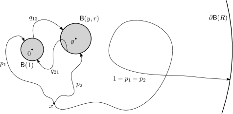
Figure 4: On the proof of Lemma 3.7

Using Lemma 3.2, we obtain

$$h_{1} =1-\frac{\ln\|x\|}{\ln R},$$ (3.22)

$$h_{2} =1-\frac{\ln\|x-y\|-\ln r}{\ln R-\ln r+O(R^{-1}\|y\|)},$$ (3.23)

and

$$q_{12} =1-\frac{\ln\|y\|-\ln r+O(\Psi_{1})}{\ln R-\ln r+O(R^{-1}\|y\|)},$$ (3.24)

$$q_{21} =1-\frac{\ln\|y\|+O(\Psi_{0})}{\ln R},$$ (3.25)

using (2.2) for the last line. Then, we use the fact that, in general,

$$h_{1} =p_{1}+p_{2}q_{21},$$

$$h_{2} =p_{2}+p_{1}q_{12},$$

and therefore

$$p_{1} =\frac{h_{1}-h_{2}q_{21}}{1-q_{12}q_{21}},$$ (3.26)

$$p_{2} =\frac{h_{2}-h_{1}q_{12}}{1-q_{12}q_{21}}.$$ (3.27)

We then write

$${\mathbb{P}}_{x}[\tau(y,r)<\tau(R)\mid\tau(1)>\tau(R)]=\frac{p_{2}(1-q_{21})}{1-h_{1}}=\frac{(1-q_{21})(h_{2}-h_{1}q_{12})}{(1-h_{1})(1-q_{12}q_{21})}.$$ (3.28)

Note that (3.22)–(3.25) imply that

$$(1-h_{1})\ln R =\ln\|x\|,$$ (3.29)

$$\lim_{R\to\infty}(1-h_{2})\ln R =\ln\|x-y\|-\ln r,$$ (3.30)

$$\lim_{R\to\infty}(1-q_{21})\ln R =\ln\|y\|+O(\Psi_{0}),$$ (3.31)

$$\lim_{R\to\infty}(1-q_{12}q_{21})\ln R =2\ln\|y\|-\ln r+O(\Psi_{1}),$$ (3.32)

$$\lim_{R\to\infty}(h_{2}-h_{1}q_{12})\ln R =\ln\|x\|+\ln\|y\|-\ln\|x-y\|+O(\Psi_{1}),$$ (3.33)

$$\lim_{R\to\infty}(h_{1}-h_{2}q_{21})\ln R =\ln\|x-y\|-\ln\|x\|+\ln\|y\|-\ln r+O(\Psi_{0}).$$ (3.34)

We then plug (3.29)–(3.33) into (3.28) and send $R$ to infinity to obtain (3.18). The proof of (3.19) is quite analogous (one needs to use (3.11) there; note also that we indirectly assume in (ii) that $r\geq 1$).

Part (iii). Next, we prove (3.20). By (3.8), we can write for any $z$ such that $\|y-z\|\leq\|y-x\|$

$$\Big{|}\frac{dH(z,\cdot)}{dH(y,\cdot)}-1\Big{|}\leq O\Big{(}\frac{\|x-y\|}{\|y\|-1}\Big{)}.$$ (3.35)

Then, a last-exit-decomposition argument implies that

$$\Big{|}\frac{d\nu_{1}}{dH(y,\cdot)}-1\Big{|}\leq O\Big{(}\frac{\|x-y\|}{\|y\|-1}\Big{)}+O\big{(}(\ln R)^{-1}\big{)}.$$ (3.36)

We then write

$$1-q_{12} =\int_{\partial{\mathsf{B}}(1)}\frac{\ln\|y-z\|-\ln r}{\ln R-\ln r+O(R^{-1}\|y\|)}\,d\nu_{1}(z)$$

$$=\int_{\partial{\mathsf{B}}(1)}\frac{\ln\|y-z\|-\ln r}{\ln R-\ln r+O(R^{-1}\|y\|)}\Big{(}O\Big{(}\frac{\|x-y\|}{\|y\|-1}\Big{)}+O\big{(}(\ln R)^{-1}\big{)}\Big{)}H(y,dz)$$

$$=\frac{\ell_{y}-\ln r}{\ln R-\ln r+O(R^{-1}\|y\|)}\Big{(}O\Big{(}\frac{\|x-y\|}{\|y\|-1}\Big{)}+O\big{(}(\ln R)^{-1}\big{)}\Big{)}.$$

Then, we obtain the following refinements of (3.32)–(3.33):

$$\lim_{R\to\infty}(1-q_{12}q_{21})\ln R =\Big{(}1+O\Big{(}\frac{\|x-y\|}{\|y\|-1}\Big{)}\Big{)}(\ln r^{-1}+\ell_{y})+\ln\|y\|+O(\Psi_{0}),$$ (3.37)

$$\lim_{R\to\infty}(h_{2}-h_{1}q_{12})\ln R =\ell_{y}+\ln\|x\|-\ln\|x-y\|+O(\Psi_{4}).$$ (3.38)

As before, the claim then follows from (3.28) (note that $\ln\|x\|-\ln\|y\|=O(\|x-y\|)$).

Part (iv). Finally, we prove (3.21). Recalling notations introduced just before Lemma 3.3, we denote for short ${\tilde{\nu}}_{x}(\cdot)=\nu_{{\mathsf{B}}(1),x}^{0,R}$ the entrance measure into ${\mathsf{B}}(1)$ starting from $x$ conditioned on $\{\tau(1)<\tau(R)\}$, and $\mu=\mu_{1}$ the uniform law on the circle. Notice that (3.5) implies

$${\tilde{\nu}}_{x}(\cdot)=\mu(\cdot)\big{(}1+O(\|x\|^{-1})\big{)},$$

and, on the other hand

$${\tilde{\nu}}_{x}(\cdot)=(1-p_{2})\nu_{1}(\cdot)+p_{2}H(y,\cdot)\big{(}1+O\big{(}\textstyle\frac{r}{\|y\|-1}\big{)}\big{)}.$$

We thus obtain

$$\nu_{1}(\cdot)=\frac{1}{1-p_{2}}\Big{(}\mu(\cdot)\big{(}1+O(\|x\|^{-1})\big{)}-p_{2}H(y,\cdot)\big{(}1+O\big{(}\textstyle\frac{r}{\|y\|-1}\big{)}\big{)}\Big{)}.$$ (3.39)

Using Lemma 3.2 and Proposition 3.1 in the definition of $q_{12}$, we obtain

$$\lim_{R\to\infty}(1-q_{12})\ln R=\ln r^{-1}+\frac{1}{1-p_{2}}\Big{(}\big{(}1+O(\|x\|^{-1})\ln\|y\|-p_{2}\ell_{y}\big{(}1+O\big{(}\textstyle\frac{r}{\|y\|-1}\big{)}\big{)}\Big{)}.$$ (3.40)

We then recall the expression (3.27) to obtain that

$$p_{2}=\frac{O\big{(}\frac{\|y\|}{|x\|}\big{)}+\frac{1}{1-p_{2}}\big{[}\ln\|y\|\big{(}1+O(\|x\|^{-1})\big{)}-p_{2}\ell_{y}\big{(}1+O\big{(}\textstyle\frac{r}{\|y\|-1}\big{)}\big{)}\big{]}}{\ln\|y\|+\ln r^{-1}+O\big{(}\frac{r}{\|y\|}\big{)}+\frac{1}{1-p_{2}}\big{[}\ln\|y\|\big{(}1+O(\|x\|^{-1})\big{)}-p_{2}\ell_{y}\big{(}1+O\big{(}\textstyle\frac{r}{\|y\|-1}\big{)}\big{)}\big{]}},$$

which can be rewritten as

$$p_{2}=\frac{a-bp_{2}}{c-dp_{2}},$$ (3.41)

where, being ${\hat{\ell}}=\ell_{y}\big{(}1+O\big{(}\textstyle\frac{r}{\|y\|-1}\big{)}\big{)}$ and $w=\ln\|y\|\big{(}1+O(\|x\|^{-1}))$,

$$a =w+O\big{(}\textstyle\frac{\|y\|}{\|x\|}\big{)},$$

$$b ={\hat{\ell}},$$

$$c =w+\ln r^{-1}+\ln\|y\|+O\big{(}\textstyle\frac{r}{\|y\|}\big{)},$$

$$d ={\hat{\ell}}+\ln\|y\|+\ln r^{-1}$$

(we need to keep track of the expressions which are exactly equal, not only up to $O$’s). We then solve (3.41) to obtain

$$p_{2}=\frac{(b+c)-\sqrt{(b+c)^{2}-4ad}}{2d}.$$

Note also that $\ln r^{-1}+\ell_{y}=O(\ln\frac{\|y\|-1}{r})$. Then, after some elementary (but long) computations one can obtain that

$$\sqrt{(b+c)^{2}-4ad}=(\ell_{y}+\ln r^{-1})(1+O(\Psi_{5}+\Psi_{7})),$$

which yields

$$p_{2}=\frac{\ln\|y\|+O(\Psi_{5}+\Psi_{7})}{\ln r^{-1}+\ln\|y\|+\ell_{y}+O(\Psi_{6})}.$$ (3.42)

We use (3.28), (3.29), and (3.31) to conclude the proof of Lemma 3.7. ∎

3.2 Some geometric properties of $\widehat{W}$ and the Wiener moustache

For two stochastic processes $X^{(1)},X^{(2)}$, we say that they coincide trajectory-wise if there exists a monotone (increasing or decreasing) stochastic process $\sigma$ such that a.s. it holds that $X^{(1)}_{\sigma(t)}=X^{(2)}_{t}$ for all $t$.

Recall that, in Remark 2.5, we denoted by $\widehat{W}^{r}$ the Brownian motion conditioned on never hitting ${\mathsf{B}}(r)$, for $r>0$; also, it can be constructed as a time change of $r\widehat{W}$. Proposition 2.3 implies that $\widehat{W}^{r}$ can be seen as $\widehat{W}$ conditioned on never hitting ${\mathsf{B}}(r)$, i.e.,

$${\mathbb{P}}_{x}\big{[}\widehat{W}_{[0,\widehat{\tau}(R)]}\in\cdot\mid\widehat{\tau}(R)<\widehat{\tau}(r)\big{]}={\mathbb{P}}_{x}\big{[}\widehat{W}^{r}_{[0,\widehat{\tau}^{r}(R)]}\in\cdot\,\big{]}$$ (3.43)

for any $R>r$ and any $x$ such that $r\leq\|x\|<R$ (we have denoted $\widehat{\tau}^{r}(R)=\inf\{t\geq 0:\widehat{W}^{r}_{t}\geq R\}$).

Using the above fact, we can prove the following lemma:

Lemma 3.9.

Let $\zeta$ be a random point with uniform distribution on $\partial{\mathsf{B}}(1)$ and let us fix $r_{0}>1$. For $t\geq 0$ define $V_{-t}=r_{0}\widehat{W}^{(1)}_{t}$, $V_{t}=\widehat{W}^{(2)}_{t}$, where $\widehat{W}^{(1,2)}$ are two independent conditioned (on not hitting ${\mathsf{B}}(1)$) Brownian motions started from $\zeta$ and $r_{0}\zeta$ correspondingly. Denote

$${\mathcal{Q}}=\inf_{t\in{\mathbb{R}}}\|V_{t}\|=\inf_{t>0}\|\widehat{W}^{(2)}_{t}\|.$$

Let $\eta$ be an instance of Wiener moustache, as in Definition 2.4. Then, for all $r_{0}>1$ and $h\in(1,r_{0})$, the law of $h\times\eta$ is a regular version of the conditional law of $V_{\mathbb{R}}$ given ${\mathcal{Q}}=h$.

In other words, the range $V_{{\mathbb{R}}}$ has same law as an independent product ${\mathcal{Q}}\times\eta$ of a Wiener moustache $\eta$ and a random variable ${\mathcal{Q}}$ distributed as in (3.44).

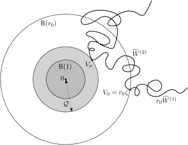
Figure 5: On the proof of Lemma 3.9

Proof.

The idea is to split $(V_{t})_{t\geq 0}$ at its minimum distance from the origin. We use polar coordinates, and let us first study the radius ${\mathcal{R}}_{t}=\|V_{t}\|$, starting with $t\in{\mathbb{R}}^{+}$. From (2.17) we derive the density of the minimal distance to the origin,

$${\mathcal{Q}}=\min\{{\mathcal{R}}_{t};t\geq 0\}\sim\frac{1}{h\ln r_{0}}\mathbf{1}_{[1,r_{0}]}(h)dh.$$ (3.44)

Applying general techniques of path decomposition [42, Theorem 2.4] to the one-dimensional diffusion ${\mathcal{R}}_{t}$, we obtain that

• there a.s. exists a unique random time $\sigma\in(0,{\infty})$ such that ${\mathcal{R}}_{\sigma}={\mathcal{Q}}$;

• given ${\mathcal{Q}}$ and $\sigma$, the process $({\mathcal{R}}_{t},t\in[0,\sigma])$ has the same law as the diffusion ${\mathcal{R}}$ started at $r_{0}$ and conditioned to converge to 1, observed up to the time of first hit of ${\mathcal{Q}}$;

• given ${\mathcal{Q}},\sigma$ and $({\mathcal{R}}_{t},t\in[0,\sigma])$, the process $({\mathcal{R}}_{\sigma+t},t\geq 0)$ has the same law as the diffusion ${\mathcal{R}}$ started at ${\mathcal{Q}}$ and conditioned on staying in $[{\mathcal{Q}},{\infty})$.

We recall that conditional diffusions are rigorously defined as in (2.13), (2.14). By the scaling property (iv) of Proposition 2.3, we see that the conditioned diffusion in (c) has the same law as an independent product ${\mathcal{Q}}\times({\mathcal{R}}_{t};t\geq 0)$ with ${\mathcal{R}}_{0}=1$. For the conditioned diffusion in (b), we use the reversibility property (ii) of Proposition 2.3: Given ${\mathcal{Q}}$ and $\sigma$,

$$\big{(}{\mathcal{R}}_{\sigma-t},t\in[0,\sigma]\big{)}\stackrel{{\scriptstyle\text{\tiny law}}}{{=}}\big{(}{\mathcal{R}}_{t}^{\prime},t\in[0,L_{r_{0}}^{\prime}]\big{)}\;,$$

where ${\mathcal{R}}^{\prime}$ is an independent ${\mathcal{R}}$-process (i.e., the norm of Brownian motion conditioned to be at least ${\mathcal{Q}}$) starting from ${\mathcal{Q}}$ and where $L_{r_{0}}^{\prime}=\sup\{t\geq 0:{\mathcal{R}}_{t}^{\prime}=r_{0}\}$ is the last exit time of ${\mathcal{R}}^{\prime}$ from $r_{0}$. Pasting it with the (independent) piece for negative times we define a new process,

$$X_{t}=\begin{cases}{\mathcal{R}}_{\sigma-t},&t\in[0,\sigma],\\ r_{0}\big{\|}\widehat{W}^{(1)}_{t-\sigma}\big{\|},\vphantom{\int\limits^{A}}&t>\sigma,\end{cases}$$

which has the same law as the above process ${\mathcal{R}}^{\prime}$. By (c), the processes $({\mathcal{R}}_{\sigma+t},t\geq 0)$ and $X$ are independent given ${\mathcal{Q}}$.

Now we consider the two-dimensional process $V$. By rotational invariance, it is clear that ${\mathcal{Q}}^{-1}V_{\sigma}$ is uniformly distributed on $\partial{\mathsf{B}}(1)$. Once the norm $\|V_{t}\|$ is defined for all $t$, one uses an independent Brownian motion and the SDE (2.12) to construct the angle process $(\Theta_{t};t\in{\mathbb{R}})$. Given the angle $\Theta_{\sigma}$, it holds that $(\Theta_{t};t\geq 0)$ and $(\Theta_{-t};t\geq 0)$ are independent with same distribution as in (2.12).

Finally, $(V_{\sigma+t};t\geq 0)$ and $(V_{\sigma-t};t\geq 0)$ are independent conditionally on $V_{\sigma}$, and both distributed as $\|V_{\sigma}\|\times\widehat{W}$. This concludes the proof. ∎

3.3 Harmonic measure and capacities

First, we need an expression on the harmonic measure $\mathop{\widehat{\mathrm{hm}}}\nolimits_{A}$ with respect to the diffusion $\widehat{W}$.

Lemma 3.10.

Assume that ${\mathsf{B}}(1)\subset A$ and let $M$ be a measurable subset of $\partial A$. We have

$${\widehat{\mathop{\mathrm{hm}}\nolimits}}_{A}(M)=\frac{\int_{M}\ln\|y\|\,d\mathop{\mathrm{hm}}\nolimits_{A}(y)}{\int_{\partial A}\ln\|y\|\,d\mathop{\mathrm{hm}}\nolimits_{A}(y)},$$ (3.45)

that is, $\mathop{\widehat{\mathrm{hm}}}\nolimits_{A}$ is $\mathop{\mathrm{hm}}\nolimits_{A}$ biased by logarithm of the distance to the origin.

Proof.

Let $\nu^{R}_{A,x}:=\nu^{0,R}_{A,x}$ be the conditional entrance measure to $A$ starting at $x\in{\mathsf{B}}(R)\setminus A$, given that $\tau(A)<\tau(R)$. For $M\subset\partial A$ we can write, using Lemma 2.1,

$${\mathbb{P}}_{x}\big{[}\widehat{W}_{\widehat{\tau}(A)}\in M\mid\widehat{\tau}(A)<\widehat{\tau}(R)\big{]} =\frac{{\mathbb{P}}_{x}[W_{\tau(A)}\in M,\tau(A)<\tau(R)<\tau(1)]}{{\mathbb{P}}_{x}[\tau(A)<\tau(R)<\tau(1)]}$$

$$=\frac{{\mathbb{P}}_{x}[W_{\tau(A)}\in M,\tau(R)<\tau(1)\mid\tau(A)<\tau(R)]}{{\mathbb{P}}_{x}[\tau(R)<\tau(1)\mid\tau(A)<\tau(R)]}$$

$$=\frac{\int_{M}\ln\|y\|\,d\nu^{R}_{A,x}(y)}{\int_{\partial A}\ln\|y\|\,d\nu^{R}_{A,x}(y)}$$ (3.46)

(observe that, by (2.2), one has to integrate $\frac{\ln\|y\|}{\ln R}$ with respect to $\nu^{R}_{A,x}$, and then the term $\ln R$ cancels). So, using (3.5) we obtain (3.45). ∎

Before proceeding, let us notice the following immediate consequence of (3.15): for any bounded $A\subset{\mathbb{R}}^{2}$ such that ${\mathsf{B}}(1)\subset A$, we have

$$\mathop{\mathrm{cap}}(A)=\lim_{\|x\|\to\infty}\frac{2}{\pi}\ln\|x\|{\mathbb{P}}_{x}[\widehat{\tau}(A)<\infty].$$ (3.47)

Next, we need estimates for the capacity of a union of ${\mathsf{B}}(1)$ with a “distant” set (in particular, a disk), and also that of a disjoint union of the unit disk and a set.

Lemma 3.11.

Assume that $\|y\|>r+1$.

• We have

  $$\mathop{\mathrm{cap}}\big{(}{\mathsf{B}}(1)\cup{\mathsf{B}}(y,r)\big{)}=\frac{2}{\pi}\cdot\frac{\ln^{2}\|y\|+O(\|y\|^{-1}(r+1)\ln\|y\|)}{2\ln\|y\|-\ln r+O(\|y\|^{-1}(r+1))}.$$ (3.48)

• For any set $A$ such that ${\mathsf{B}}(y,1)\subset A\subset{\mathsf{B}}(y,r)$, we have

  $$\mathop{\mathrm{cap}}\big{(}{\mathsf{B}}(1)\cup A\big{)}=\frac{2}{\pi}\cdot\mathop{\mathrm{cap}}\big{(}{\mathsf{B}}(1)\cup A\big{)}=\frac{2}{\pi}\cdot\frac{\ln^{2}\|y\|+O(\|y\|^{-1}r\ln\|y\|\ln r)}{2\ln\|y\|-\frac{\pi}{2}\mathop{\mathrm{cap}}({\mathcal{T}}_{-y}A)+O(\|y\|^{-1}r)}.$$ (3.49)

  with ${\mathcal{T}}_{y}$ the translation by vector $y$.

• Moreover, we have the following refinement of (3.48)

  $$\mathop{\mathrm{cap}}\big{(}{\mathsf{B}}(1)\cup{\mathsf{B}}(y,r)\big{)}=\frac{2}{\pi}\cdot\frac{(\ln\|y\|+O(\Psi_{0}))(\ln\|y\|+O(\Psi_{5}+\Psi_{7}))}{\ln r^{-1}+\ell_{y}+\ln\|y\|+O(\Psi_{6})}$$ (3.50)

  with $\Psi_{0},\Psi_{5},\Psi_{6},\Psi_{7}$ as in Lemma 3.7.

Proof.

All these expressions follow from (3.47) and Lemma 3.7. ∎

We also need to estimates the capacity of a union of two overlapping disks. We first consider a (typically small) disk with center on the boundary of ${\mathsf{B}}(1)$.

Lemma 3.12.

For any $x\in\partial{\mathsf{B}}(1)$ and $r\in(0,2)$ it holds that

$$\mathop{\mathrm{cap}}\big{(}{\mathsf{B}}(1)\cup{\mathsf{B}}(x,r)\big{)} =\frac{2}{\pi}\ln\frac{2\sin(\pi\varphi)}{(1+\varphi)\sin(\pi\frac{1-\varphi}{1+\varphi})}$$ (3.51)

$$=\frac{r^{2}}{\pi}(1+O(r))\quad\text{ as $r\to 0$,}$$

where $\varphi=\frac{2}{\pi}\arcsin\frac{r}{2}$.

Proof.

Clearly, without loss of generality one may assume that $x=1$; let us abbreviate $A_{r}={\mathsf{B}}(1)\cup{\mathsf{B}}(1,r)$. We intend to use Theorem 5.2.3 of [33]; for that, we need to find a conformal mapping $f$ of ${\mathbb{C}}_{\infty}\setminus A_{r}$ onto ${\mathbb{C}}_{\infty}\setminus{\mathsf{B}}(s)$, which sends $\infty$ to $\infty$ and such that $f(z)=z+O(1)$ as $z\to\infty$, where $s>1$ (and then Theorem 5.2.3 of [33] will imply that the capacities of $A_{r}$ and ${\mathsf{B}}(s)$ are equal). Clearly, for this it is enough to map ${\mathbb{C}}_{\infty}\setminus A_{r}$ onto ${\mathbb{C}}_{\infty}\setminus{\mathsf{B}}(1)$ with $f$ such that $f(z)=cz+O(1)$, where $|c|\in(0,1)$, and then normalize. That is, we then obtain that $c^{-1}f$ sends ${\mathbb{C}}_{\infty}\setminus A_{r}$ onto ${\mathbb{C}}_{\infty}\setminus{\mathsf{B}}(|c|^{-1})$, which would give that $\mathop{\mathrm{cap}}(A_{r})=\frac{2}{\pi}\ln|c|^{-1}$.

First, it is elementary to obtain that $\partial{\mathsf{B}}(1)$ and $\partial{\mathsf{B}}(1,r)$ intersect in the points $e^{i\pi\varphi}$ and $e^{-i\pi\varphi}$. We then apply the map

$$f_{1}(z)=\frac{z-e^{i\pi\varphi}}{z-e^{-i\pi\varphi}},$$ (3.52)

which sends the first of these points to $0$ and the second to $\infty$. Observe also that $f_{1}(\infty)=1$. Since $f_{1}$ is a Möbius transformation, it sends the two arcs that form $\partial A_{r}$ into two rays, and therefore ${\mathbb{C}}_{\infty}\setminus A_{r}$ gets mapped to a sector. The tangent vectors $v_{1,2}$ to the two arcs at $e^{i\pi\varphi}$ have directions $\frac{\pi}{2}+\pi\varphi$ and $\frac{\pi\varphi}{2}$ (see Figure 6), so the angle of that sector is $\frac{\pi}{2}+\pi\varphi-\frac{\pi\varphi}{2}=\frac{\pi}{2}(\varphi+1)$.

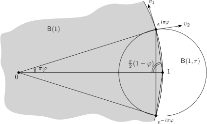
Figure 6: The direction of vector $v_{1}$ is $\frac{\pi}{2}+\pi\varphi$, and the direction of vector $v_{2}$ is $\frac{\pi\varphi}{2}$.

To see what are the directions of these two rays, observe that

$$f^{\prime}_{1}(z)=\frac{e^{i\pi\varphi}-e^{-i\pi\varphi}}{(z-e^{-i\pi\varphi})^{2}},$$

so $f^{\prime}_{1}(e^{i\pi\varphi})=(e^{i\pi\varphi}-e^{-i\pi\varphi})^{-1}=\frac{-i}{2\sin\pi\varphi}$. This means that, at point $e^{i\pi\varphi}$, the map $f_{1}$ rotates $\frac{\pi}{2}$ clockwise, and so the direction of the first ray is $\pi\varphi$ and the direction of the second one is $(-i\frac{\pi}{2}(1-\varphi))$.

Next, we apply the function

$$z\mapsto\big{(}e^{i\frac{\pi}{2}(1-\varphi)}z\big{)}^{\frac{2}{1+\varphi}}$$

to send this sector to the upper half-plane (we first rotate the sector so that its right boundary goes to the positive part of the horizontal axis, and then “open” it so that its angle changes from $\frac{\pi}{2}(\varphi+1)$ to $\pi$). The point $1$ (the image of $\infty$ under $f_{1}$) is then sent to $e^{i\pi\frac{1-\varphi}{1+\varphi}}$. Then, we need to map the upper half plane to ${\mathbb{C}}_{\infty}\setminus{\mathsf{B}}(1)$ in such a way that $e^{i\pi\frac{1-\varphi}{1+\varphi}}$ is sent back to $\infty$. This is achieved by the function

$$z\mapsto\frac{z-e^{-i\pi\frac{1-\varphi}{1+\varphi}}}{z-e^{i\pi\frac{1-\varphi}{1+\varphi}}}.$$

Gathering the pieces, we then obtain that the map

$$f(z)=\frac{\big{(}e^{i\frac{\pi}{2}(1-\varphi)}\frac{z-e^{i\pi\varphi}}{z-e^{-i\pi\varphi}}\big{)}^{\frac{2}{1+\varphi}}-e^{-i\pi\frac{1-\varphi}{1+\varphi}}}{\big{(}e^{i\frac{\pi}{2}(1-\varphi)}\frac{z-e^{i\pi\varphi}}{z-e^{-i\pi\varphi}}\big{)}^{\frac{2}{1+\varphi}}-e^{i\pi\frac{1-\varphi}{1+\varphi}}}$$ (3.53)

sends ${\mathbb{C}}_{\infty}\setminus A_{r}$ to ${\mathbb{C}}_{\infty}\setminus{\mathsf{B}}(1)$.

Next, we need to obtain the asymptotic behavior of the above function as $z\to\infty$. First, it clearly holds that

$$\Big{|}\Big{(}e^{i\frac{\pi}{2}(1-\varphi)}\frac{z-e^{i\pi\varphi}}{z-e^{-i\pi\varphi}}\Big{)}^{\frac{2}{1+\varphi}}-e^{-i\pi\frac{1-\varphi}{1+\varphi}}\Big{|}\to\Big{|}e^{i\pi\frac{1-\varphi}{1+\varphi}}-e^{-i\pi\frac{1-\varphi}{1+\varphi}}\Big{|}=2\sin\big{(}\pi\textstyle\frac{1-\varphi}{1+\varphi}\big{)}\quad\text{ as }z\to\infty.$$ (3.54)

We have

$$\frac{z-e^{i\pi\varphi}}{z-e^{-i\pi\varphi}}=\frac{1-e^{i\pi\varphi}z^{-1}}{1-e^{-i\pi\varphi}z^{-1}}=1-(e^{i\pi\varphi}-e^{-i\pi\varphi})z^{-1}+O(z^{-2})=1-2i\sin(\pi\varphi)z^{-1}+O(z^{-2}),$$

so, we can write

$$\lim_{z\to\infty}|z|\cdot\Big{|}\Big{(}e^{i\frac{\pi}{2}(1-\varphi)}\frac{z-e^{i\pi\varphi}}{z-e^{-i\pi\varphi}}\Big{)}^{\frac{2}{1+\varphi}}-e^{i\pi\frac{1-\varphi}{1+\varphi}}\Big{|}$$

$$=\lim_{z\to\infty}|z|\cdot\Big{|}\big{(}1-2i\sin(\pi\varphi)z^{-1}+O(z^{-2})\big{)}^{\frac{2}{1+\varphi}}-1\Big{|}$$

$$=\frac{4\sin(\pi\varphi)}{1+\varphi}.$$ (3.55)

The relations (3.54)–(3.55) imply that the function in (3.53) is $f(z)=cz+O(1)$ with

$$|c|=2\sin\big{(}\pi{\textstyle\frac{1-\varphi}{1+\varphi}}\big{)}\Big{(}\frac{4\sin(\pi\varphi)}{1+\varphi}\Big{)}^{-1}=\frac{(1+\varphi)\sin(\pi\frac{1-\varphi}{1+\varphi})}{2\sin(\pi\varphi)}.$$

This gives the exact formula in (3.51), and then one obtains the asymptotic expression as $r\to 0$ with a straightforward calculation. ∎

Also, we treat the case when the center of the second disk is in the interior of the first one.

Lemma 3.13.

For $\|x\|\in(0,1)$ and $r\in(1-\|x\|,1+\|x\|)$ it holds that

$$\mathop{\mathrm{cap}}\big{(}{\mathsf{B}}(1)\cup{\mathsf{B}}(x,r)\big{)} =\frac{2}{\pi}\ln\frac{\sin(\pi\varphi)}{(1\!+\!\varphi\!-\!\psi)\sin\frac{\pi\varphi}{1\!+\!\varphi\!-\!\psi}}$$ (3.56)

$$=\frac{4\sqrt{2}}{3\pi^{2}}\sqrt{\frac{1\!-\!\|x\|}{\|x\|}}h^{3/2}+O(h^{2})$$

as $h:=r-(1-\|x\|)\searrow 0$, where

$$\varphi=\frac{2}{\pi}\arcsin\Bigg{(}\frac{1}{2}\sqrt{\frac{r^{2}-(1-\|x\|)^{2}}{\|x\|}}\Bigg{)}\;,\qquad\psi=\frac{2}{\pi}\arcsin\Bigg{(}\frac{1}{2}\sqrt{\frac{(r+\|x\|)^{2}-1}{r\|x\|}}\Bigg{)}\;.$$

One can check that, at $\|x\|=1$, (3.56) matches (3.51).

Proof.

We proceed exactly as in the proof of Lemma 3.12. Without loss of generality we assume that $x$ is on the positive semi-axis. We parametrize the intersection points of $\partial{\mathsf{B}}(1)$ and $\partial{\mathsf{B}}(x,r)$ by their angles $\pm\pi\hat{\varphi}$ as seen from the origin and $\pm\pi\hat{\psi}$ as seen from the point $x$. Writing the identity $e^{i\pi\hat{\varphi}}=x+re^{i\pi\hat{\psi}}$ in terms of $\sin(\pi\hat{\varphi}/2),\sin(\pi\hat{\psi}/2)$, we obtain that $\hat{\varphi}=\varphi$ and $\hat{\psi}=\psi$ with $\varphi,\psi$ defined in the Lemma. The tangent vectors $v_{1,2}$ at point $e^{i\pi\varphi}$ now have directions $\pi(\varphi+1/2)$ and $\pi(\psi-1/2)$, so the sector has angle $\pi(1+\varphi-\psi)$. Applying the map $f_{1}$ from (3.52), the domain ${\mathbb{C}}_{\infty}\setminus A_{r}$ gets mapped to the sector determined the rays $e^{i\pi\varphi}$ and $e^{-i\pi(1-\psi)}$ containing the point 1. Next we apply the function

$$z\mapsto e^{i\pi\frac{1-\psi}{1+\varphi-\psi}}z^{\frac{1}{1+\varphi-\psi}}$$

which maps this sector to the upper half-plane. Finally we compose with the function $z\mapsto\frac{z-\bar{a}}{z-a}$ with $a=e^{i\pi\frac{1-\psi}{1+\varphi-\psi}}$, i.e., the image of 1 by the previous function.

Collecting the pieces, we then obtain that the map

$$f(z)=\frac{\big{(}\frac{z-e^{i\pi\varphi}}{z-e^{-i\pi\varphi}}\big{)}^{\frac{1}{1+\varphi-\psi}}-e^{-2i\pi\frac{1-\psi}{1+\varphi-\psi}}}{\big{(}\frac{z-e^{i\pi\varphi}}{z-e^{-i\pi\varphi}}\big{)}^{\frac{1}{1+\varphi-\psi}}-1}$$ (3.57)

sends ${\mathbb{C}}_{\infty}\setminus A_{r}$ to ${\mathbb{C}}_{\infty}\setminus{\mathsf{B}}(1)$.

Next, we expand the above function at $\infty$:

$$\Big{(}\frac{z-e^{i\pi\varphi}}{z-e^{-i\pi\varphi}}\Big{)}^{\frac{1}{1+\varphi-\psi}}=1-\frac{2i\sin(\pi\varphi)}{1+\varphi-\psi}z^{-1}+O(z^{-2}),$$

yielding, as $z\to\infty$,

$${}f(z)=cz+O(1)\;,\qquad c=\frac{i(1+\varphi-\psi)}{2\sin(\pi\varphi)}\big{(}1-e^{-2i\pi\frac{1-\psi}{1+\varphi-\psi}}\big{)}\;,$$

and so

$$|c| =\frac{(1+\varphi-\psi)}{\sin(\pi\varphi)}\sin\big{(}\pi\frac{1-\psi}{1+\varphi-\psi}\big{)}$$

$$=\frac{(1+\varphi-\psi)}{\sin(\pi\varphi)}\sin\big{(}\pi\frac{\varphi}{1+\varphi-\psi}\big{)}.$$

This gives the exact formula in (3.56). Then, the asymptotic expression as $r\to 1-\|x\|$ follows from a tedious expansion. ∎

Next, we need a formula for the capacity of a union of three unit disks; note that, unlike the discrete case (see Lemma 3.8 in [13]), in the continuous setting there is no closed-form exact expression for this capacity (at least the authors are unaware of such).

Lemma 3.14.

For $y,z$ such that the disks ${\mathsf{B}}(1),{\mathsf{B}}(y,1),{\mathsf{B}}(z,1)$ are disjoint, abbreviate $A={\mathsf{B}}(1)\cup{\mathsf{B}}(y,1)\cup{\mathsf{B}}(z,1)$ and $a=\ln\|y\|$, $b=\ln\|z\|$, $c=\ln\|y-z\|$. Assume that, for some fixed $\varepsilon_{0}>0$, it holds that $\min\{a,b,c\}\geq\varepsilon_{0}\max\{a,b,c\}$. Then, we have

$$\mathop{\mathrm{cap}}(A)=\frac{2}{\pi}\cdot\frac{2abc+O\big{(}\frac{\ln^{2}(a\vee b\vee c)}{a\wedge b\wedge c}\big{)}}{2(ab+ac+bc)-(a^{2}+b^{2}+c^{2})+O\big{(}\frac{\ln(a\vee b\vee c)}{a\wedge b\wedge c}\big{)}}.$$ (3.58)

Proof.

Let $r=\lceil\|y\|\vee\|z\|\rceil+1$, and observe that $A\subset{\mathsf{B}}(r)$. The idea is to use (3.11) with $x=(r^{3},0)$ (so that $\ln\|x\|=3\ln r$) and $R=r^{5}$. In this situation, (3.11) implies that

$$\frac{\pi}{2}\mathop{\mathrm{cap}}(A)=\Big{(}1-\frac{2+O\big{(}\frac{1}{r^{2}}\big{)}}{5{\mathbb{P}}_{x}[\tau(A)<\tau(R)]}\Big{)}\ln R+O\big{(}\textstyle\frac{\ln r}{r^{2}}\big{)}.$$ (3.59)

Then, we proceed similarly to the proof of Lemma 3.7. Let

$$p_{1} ={\mathbb{P}}_{x}\big{[}\tau(A)<\tau(R),\tau(A)=\tau({\mathsf{B}}(1))\big{]},$$

$$p_{2} ={\mathbb{P}}_{x}\big{[}\tau(A)<\tau(R),\tau(A)=\tau({\mathsf{B}}(y,1))\big{]},$$

$$p_{3} ={\mathbb{P}}_{x}\big{[}\tau(A)<\tau(R),\tau(A)=\tau({\mathsf{B}}(z,1))\big{]},$$

so ${\mathbb{P}}_{x}[\tau(A)<\tau(R)]=p_{1}+p_{2}+p_{3}$. Next, denote (recall (3.3))

$$h_{1} ={\mathbb{P}}_{x}\big{[}\tau({\mathsf{B}}(1))<\tau(R)\big{]}=\frac{2}{5},$$

$$h_{2} ={\mathbb{P}}_{x}\big{[}\tau({\mathsf{B}}(y,1))<\tau(R)\big{]}=\frac{2}{5}\big{(}1+O\big{(}\textstyle\frac{1}{r^{2}\ln r}\big{)}\big{)},$$

$$h_{3} ={\mathbb{P}}_{x}\big{[}\tau({\mathsf{B}}(z,1))<\tau(R)\big{]}=\frac{2}{5}\big{(}1+O\big{(}\textstyle\frac{1}{r^{2}\ln r}\big{)}\big{)},$$

(observe that $\frac{\ln\|x\|}{\ln R}=\frac{3}{5}$). Let ${\hat{a}}=a/\ln R$, ${\hat{b}}=b/\ln R$, ${\hat{c}}=c/\ln R$. Then, let us denote

$$q_{12} ={\mathbb{P}}_{\nu_{1}}\big{[}\tau({\mathsf{B}}(y,1))<\tau(R)\big{]}=1-{\hat{a}}\big{(}1+O\big{(}\textstyle\frac{1}{\|y\|\ln\|y\|}\big{)}\big{)},$$

$$q_{13} ={\mathbb{P}}_{\nu_{1}}\big{[}\tau({\mathsf{B}}(z,1))<\tau(R)\big{]}=1-{\hat{b}}\big{(}1+O\big{(}\textstyle\frac{1}{\|z\|\ln\|z\|}\big{)}\big{)},$$

$$q_{21} ={\mathbb{P}}_{\nu_{2}}\big{[}\tau({\mathsf{B}}(1))<\tau(R)\big{]}=1-{\hat{a}}\big{(}1+O\big{(}\textstyle\frac{1}{\|y\|\ln\|y\|}\big{)}\big{)},$$

$$q_{23} ={\mathbb{P}}_{\nu_{2}}\big{[}\tau({\mathsf{B}}(z,1))<\tau(R)\big{]}=1-{\hat{c}}\big{(}1+O\big{(}\textstyle\frac{1}{\|y-z\|\ln\|y-z\|}\big{)}\big{)},$$

$$q_{31} ={\mathbb{P}}_{\nu_{3}}\big{[}\tau({\mathsf{B}}(1))<\tau(R)\big{]}=1-{\hat{b}}\big{(}1+O\big{(}\textstyle\frac{1}{\|z\|\ln\|z\|}\big{)}\big{)},$$

$$q_{32} ={\mathbb{P}}_{\nu_{1}}\big{[}\tau({\mathsf{B}}(y,1))<\tau(R)\big{]}=1-{\hat{c}}\big{(}1+O\big{(}\textstyle\frac{1}{\|y-z\|\ln\|y-z\|}\big{)}\big{)},$$

where $\nu_{1}$ (respectively, $\nu_{2}$ and $\nu_{3}$) is the entrance measure to ${\mathsf{B}}(1)$ (respectively, to ${\mathsf{B}}(y,1)$ and ${\mathsf{B}}(z,1)$) conditioned on $\{\tau(1)<\tau({\mathsf{B}}(y,1))\wedge\tau({\mathsf{B}}(z,1))\wedge\tau(R)\}$ (respectively, on $\{\tau({\mathsf{B}}(y,1))<\tau(1)\wedge\tau({\mathsf{B}}(z,1))\wedge\tau(R)\}$ and $\{\tau({\mathsf{B}}(z,1))<\tau(1)\wedge\tau({\mathsf{B}}(y,1))\wedge\tau(R)\}$).

It is elementary to see that, as a general fact,

$$h_{1} =p_{1}+p_{2}q_{21}+p_{3}q_{31},$$

$$h_{2} =p_{1}q_{12}+p_{2}+p_{3}q_{32},$$

$$h_{3} =p_{1}q_{13}+p_{2}q_{23}+p_{3}.$$

Next, we solve the above system of linear equations with respect to $p_{1,2,3}$ and then use (3.59) to obtain (3.58). We omit the precise calculations which are elementary but long; however, to convince the reader that the answer is correct, let us forget for a moment about the $O$’s in the above expressions for $h$’s and $q$’s and see where it will lead us. Denote by 1 the column vector with all the coordinates being equal to $1$, and define the matrix

$$L=\begin{pmatrix}1&1-{\hat{a}}&1-{\hat{b}}\\ 1-{\hat{a}}&1&1-{\hat{c}}\\ 1-{\hat{b}}&1-{\hat{c}}&1\end{pmatrix}.$$

Let $p^{\prime}_{1,2,3}$ be the solutions of the above equations “without the $O$’s”, i.e., with $\frac{2}{5}$ on the place of $h_{1,2,3}$, and $1-{\hat{a}}$ (respectively, $1-{\hat{b}}$ and $1-{\hat{c}}$) on the place of $q_{12}$ (respectively, $q_{13}$ and $q_{23}$). Clearly, we have that $p^{\prime}_{1}+p^{\prime}_{2}+p^{\prime}_{3}=\mathbf{1}^{\mathsf{T}}L^{-1}\mathbf{1}$. Then, the right-hand side of (3.59) would become

$$\Big{(}1-\frac{1}{\mathbf{1}^{\mathsf{T}}L^{-1}\mathbf{1}}\Big{)}\ln R =\Big{(}1-\frac{2({\hat{a}}{\hat{b}}+{\hat{a}}{\hat{c}}+{\hat{b}}{\hat{c}})-({\hat{a}}^{2}+{\hat{b}}^{2}+{\hat{c}}^{2})-2{\hat{a}}{\hat{b}}{\hat{c}}}{2({\hat{a}}{\hat{b}}+{\hat{a}}{\hat{c}}+{\hat{b}}{\hat{c}})-({\hat{a}}^{2}+{\hat{b}}^{2}+{\hat{c}}^{2})}\Big{)}\ln R$$

$$=\frac{2{\hat{a}}{\hat{b}}{\hat{c}}}{2({\hat{a}}{\hat{b}}+{\hat{a}}{\hat{c}}+{\hat{b}}{\hat{c}})-({\hat{a}}^{2}+{\hat{b}}^{2}+{\hat{c}}^{2})}\ln R$$

$$=\frac{2abc}{2(ab+ac+bc)-(a^{2}+b^{2}+c^{2})},$$

which indeed agrees with (3.58). As a final remark, let us also observe that inserting the $O$’s back is not problematic, because an elementary calculation shows that $|\det L|=2({\hat{a}}{\hat{b}}+{\hat{a}}{\hat{c}}+{\hat{b}}{\hat{c}})-({\hat{a}}^{2}+{\hat{b}}^{2}+{\hat{c}}^{2})-2{\hat{a}}{\hat{b}}{\hat{c}}$ is bounded away from $0$ (note that, due to the triangle inequality, at least two of the quantities $a,b,c$ should be approximately equal to $\ln r$, and so at least two of ${\hat{a}},{\hat{b}},{\hat{c}}$ are approximately $\frac{1}{5}$; also, we assumed that the smallest of them must be bounded away from $0$). ∎

We also need to compare the harmonic measure on a set (typically distant from the origin) to the entrance measure of $\widehat{W}$ started far away from that set.

Lemma 3.15.

Assume that the compact subset $A$ of ${\mathbb{R}}^{2}$ and $x\notin{\mathsf{B}}(1)$ are such that $2\,{\mathop{\mathrm{diam}}}(A)+1<\min\!\big{(}\!\mathop{\mathrm{dist}}(x,A),\,\frac{1}{4}\mathop{\mathrm{dist}}({\mathsf{B}}(1),A)\big{)}$. Abbreviate $u={\mathop{\mathrm{diam}}}(A)$, $s=\mathop{\mathrm{dist}}(x,A)$. Assume also that $A^{\prime}\subset{\mathbb{R}}^{2}$ is compact or empty, and such that $\mathop{\mathrm{dist}}(A,A^{\prime})\geq s+1$ (for definiteness, we adopt the convention $\mathop{\mathrm{dist}}(A,\emptyset)=\infty$ for any $A$). Then, for all $M\subset\partial A$, it holds that

$${\mathbb{P}}_{x}\big{[}\widehat{W}_{\widehat{\tau}(A)}\in M\mid\widehat{\tau}(A)<\infty,\widehat{\tau}(A)<\widehat{\tau}(A^{\prime})\big{]}=\mathop{\mathrm{hm}}\nolimits_{A}(M)\Big{(}1+O\Big{(}\frac{u}{s}\Big{)}\Big{)}.$$ (3.60)

Proof.

This result is analogous to Lemma 3.10 of [13], but, since the proof of the latter contains an inaccuracy, we give the proof here, also noting that the same argument works in the discrete setting as well.

Let $z_{0}\in A$ be such that $\|z_{0}-x\|=s$, and observe that the assumptions imply that $({\mathsf{B}}(1)\cup A^{\prime})\cap{\mathsf{B}}(z_{0},s)=\emptyset$. Let us fix some $R$ such that $A\cup A^{\prime}\cup\{x\}\subset{\mathsf{B}}(R)$, and abbreviate

$$G=\big{\{}\tau(A)<\tau(A^{\prime})\wedge\tau(R),\tau(R)<\tau(1)\big{\}}.$$

Define the (possibly infinite) random variable

$$\sigma=\begin{cases}\inf\big{\{}t\geq 0:W_{t}\in{\mathsf{B}}(z_{0},{\textstyle\frac{s}{2}}),W_{[t,\tau(A)]}\cap\partial{\mathsf{B}}(z_{0},s)=\emptyset\big{\}}&\text{ on }G,\\ \infty&\text{ on }G^{\complement}\end{cases}$$

to be the moment when the last excursion between ${\mathsf{B}}(z_{0},\frac{s}{2})$ and $\partial{\mathsf{B}}(z_{0},s)$ starts; formally, we also set $W_{\sigma}=\infty$ on $\{\sigma=\infty\}$. Let us stress that $\sigma$ is not a stopping time; it was defined in such a way that the law of the excursion that begins at time $\sigma$ is the law of a Brownian excursion conditioned to reach $A$ (and then $\partial B(R)$) before going back to ${\mathsf{B}}(1)$. Let $\nu$ be the joint law of the pair $(\sigma,W_{\sigma})$ under ${\mathbb{P}}_{x}$. Abbreviate also $\mathcal{H}={\mathbb{R}}_{+}\times\partial{\mathsf{B}}(z_{0},\frac{s}{2})$ and observe that $\int_{\mathcal{H}}\,d\nu(t,y)={\mathbb{P}}_{x}[G]$.

Now, using Lemma 2.1, (2.2), and (3.5), we write

$${\mathbb{P}}_{x}\big{[}\widehat{W}_{\widehat{\tau}(A)}\in M,\widehat{\tau}(A)<\widehat{\tau}(R)\wedge\widehat{\tau}(A^{\prime})\big{]}$$

$$={\mathbb{P}}_{x}\big{[}W_{\tau(A)}\in M,\tau(A)<\tau(R)\wedge\tau(A^{\prime})\mid\tau(R)<\tau(1)\big{]}$$

$$=\frac{\ln R}{\ln\|x\|}{\mathbb{P}}_{x}\big{[}W_{\tau(A)}\in M,\tau(A)<\tau(A^{\prime})\wedge\tau(R),\tau(R)<\tau(1)\big{]}$$

$$=\frac{\ln R}{\ln\|x\|}\int_{\mathcal{H}}{\mathbb{P}}_{y}\big{[}W_{\tau(A)}\in M\mid\tau(A)<\tau\big{(}\partial{\mathsf{B}}(z_{0},{\textstyle\frac{s}{2}})\big{)}\big{]}\,d\nu(t,y)$$

$$=\frac{\ln R}{\ln\|x\|}\mathop{\mathrm{hm}}\nolimits_{A}(M)\Big{(}1+O\Big{(}\frac{u}{s}\Big{)}\Big{)}{\mathbb{P}}_{x}\big{[}\tau(A)<\tau(A^{\prime})\wedge\tau(R),\tau(R)<\tau(1)\big{]}$$

$$=\mathop{\mathrm{hm}}\nolimits_{A}(M)\Big{(}1+O\Big{(}\frac{u}{s}\Big{)}\Big{)}{\mathbb{P}}_{x}\big{[}\tau(A)<\tau(A^{\prime})\wedge\tau(R)\mid\tau(R)<\tau(1)\big{]}$$

$$=\mathop{\mathrm{hm}}\nolimits_{A}(M)\Big{(}1+O\Big{(}\frac{u}{s}\Big{)}\Big{)}{\mathbb{P}}_{x}\big{[}\widehat{\tau}(A)<\widehat{\tau}(A^{\prime})\wedge\widehat{\tau}(R)\big{]},$$

and we conclude the proof of Lemma 3.15 by sending $R$ to infinity. ∎

3.4 Excursions

In this section we define excursions of the Brownian random interlacements and the Brownian motion on the torus. The corresponding definitions for the discrete random interlacements and the simple random walk on the torus are contained in Section 3.4 of [13]; since the definitions are completely analogous in the continuous case, we make this section rather sketchy.

Consider two closed sets $A$ and $A^{\prime}$ such that $A\subset(A^{\prime})^{o}\subset{\mathbb{R}}^{2}_{n}$ (usually, they will be disks), and let $T_{n}(M)$ be the hitting time of a set $M\subset{\mathbb{R}}^{2}_{n}$ for the process $X$. By definition, an excursion $\varrho$ is a continuous (in fact, Brownian) path that starts at $\partial A$ and ends on its first visit to $\partial A^{\prime}$, i.e., $\varrho=(\varrho_{t},t\in[0,v])$, where $\varrho_{0}\in\partial A$, $\varrho_{v}\in\partial A^{\prime}$, $\varrho_{s}\notin\partial A^{\prime}$ for all $s\in[0,v)$. To define these excursions, consider the following sequence of stopping times:

$$D_{0} =T_{n}(\partial A^{\prime}),$$

$$J_{1} =\inf\{t>D_{0}:X_{t}\in\partial A\},$$

$$D_{1} =\inf\{t>J_{1}:X_{t}\in\partial A^{\prime}\},$$

and

$$J_{k} =\inf\{t>D_{k-1}:X_{t}\in\partial A\},$$

$$D_{k} =\inf\{t>J_{k}:X_{t}\in\partial A^{\prime}\},$$

for $k\geq 2$. Then, denote by $Z^{(i)}=X_{|[J_{i},D_{i}]}$ the $i$th excursion of $X$ between $\partial A$ and $\partial A^{\prime}$, for $i\geq 1$. Also, let $Z^{(0)}=X_{|[0,D_{0}]}$ be the “initial” excursion (it is possible, in fact, that it does not intersect the set $A$ at all). Recall that $t_{\alpha}:=\frac{2\alpha}{\pi}n^{2}\ln^{2}n$ and define

$$N_{\alpha} =\max\{k:J_{k}\leq t_{\alpha}\},$$ (3.61)

$$N^{\prime}_{\alpha} =\max\{k:D_{k}\leq t_{\alpha}\}$$ (3.62)

to be the number of incomplete (respectively, complete) excursions up to time $t_{\alpha}$.

Observe that, quite analogously to the above, we can define the excursions of the conditioned diffusion $\widehat{W}$ between $\partial A$ and $\partial A^{\prime}$ (this time, $A$ and $A^{\prime}$ are subsets of ${\mathbb{R}}^{2}$); since $\widehat{W}$ is transient, the number of those will be a.s. finite. Next, we also define the excursions of (Brownian) random interlacements. Suppose that the trajectories of the $\widehat{W}$-diffusions that intersect $A$ are enumerated according to the points of the generating one-dimensional Poisson process (cf. Definition 2.6). For each trajectory from that list (say, the $j$th one, denoted $\widehat{W}^{(j)}$ and time-shifted in such a way that $\widehat{W}^{(j)}_{s}\notin A$ for all $s<0$ and $\widehat{W}^{(j)}_{0}\in A$) define the stopping times

$${\hat{J}}_{1} =0,$$

$${\hat{D}}_{1} =\inf\big{\{}t>{\hat{J}}_{1}:\widehat{W}^{(j)}_{t}\in\partial A^{\prime}\big{\}},$$

and

$${\hat{J}}_{k} =\inf\big{\{}t>{\hat{D}}_{k-1}:\widehat{W}^{(j)}_{t}\in\partial A\big{\}},$$

$${\hat{D}}_{k} =\inf\big{\{}t>{\hat{J}}_{k}:\widehat{W}^{(j)}_{t}\in\partial A^{\prime}\big{\}},$$

for $k\geq 2$. Let $\ell_{j}=\inf\{k:{\hat{J}}_{k}=\infty\}-1$ be the number of excursions corresponding to the $j$th trajectory. The excursions of $\mathop{\mathrm{BRI}}(\alpha)$ between $\partial A$ and $\partial A^{\prime}$ are defined by

$$\widehat{Z}^{(i)}=\widehat{W}^{(j)}_{[{\hat{J}}_{m},{\hat{D}}_{m}]},$$

where $i=m+\sum_{k=1}^{j-1}\ell_{k}$, and $m=1,2,\ldots,\ell_{j}$. Let $R_{\alpha}$ be the number of trajectories intersecting $A$ on level $\alpha$, and denote ${\hat{N}}_{\alpha}=\sum_{k=1}^{R_{\alpha}}\ell_{k}$ to be the total number of excursions of $\mathop{\mathrm{BRI}}(\alpha)$ between $\partial A$ and $\partial A^{\prime}$.

Observe also that the above construction makes sense with $\alpha=\infty$ as well; we then obtain an infinite sequence of excursions of $\mathop{\mathrm{BRI}}$ (=$\mathop{\mathrm{BRI}}(\infty)$) between $\partial A$ and $\partial A^{\prime}$.

Next, we need to control the number of excursions between the boundaries of two concentric disks on the torus:

Lemma 3.16.

Consider the random variables $(J_{k},D_{k})$ defined in this section with $A=B(r)$ and $A^{\prime}=B(R)$. Assume that $1<r<R<\frac{n}{2}$, $m\geq 2$, and $\delta\in(0,c_{0})$ for some $c_{0}>0$. Then, there exist positive constants $c_{1},c_{2}$ such that

$${\mathbb{P}}\Big{[}J_{m}\notin\Big{(}\frac{(1\!-\!\delta)m}{\pi}n^{2}\ln\frac{R}{r},\frac{(1\!+\!\delta)m}{\pi}n^{2}\ln\frac{R}{r}\Big{)}\Big{]}\leq c_{1}\exp\Big{(}-c_{2}\delta^{2}m\frac{R\big{(}1\!-\!\frac{r}{R}\big{)}^{6}}{n\ln^{2}r^{-1}}\Big{)},$$ (3.63)

and the same result holds with $D_{m}$ on the place of $J_{m}$.

Proof.

This is Proposition 8.10 of [4], with small adaptations, since we are working with torus of size $n$ in the continuous setting as well. ∎

4 Proofs of the main results

4.1 Proof of Theorems 2.10, 2.11 and 2.13

Proof of Proposition 2.10.

We start with a preliminary observation. Consider the process $\widehat{W}$ started at some $x\in{\mathbb{R}}^{2}$ with $\|x\|=r>1$, and consider the random variable $H=\inf_{t>0}\|\widehat{W}_{t}\|$ to be the minimal distance of the trajectory to the origin; note that $H>1$ a.s.. By (2.17), it holds that ${\mathbb{P}}_{x}[H\leq s]=\frac{\ln s}{\ln r}$, so $H$ has density $f(s)=\frac{1}{s\ln r}{\mathbf{1}}_{\{s\in[1,r]\}}$. But then, using Lemma 3.9, we see that the trace of $\mathop{\mathrm{BRI}}(\alpha)$ on ${\mathsf{B}}(r)$ can be obtained in the following way: take $N\sim\text{Poisson}(2\alpha\ln r)$ particles and place them on $\partial{\mathsf{B}}(r)$ uniformly and independently; then let these particles perform independent $\widehat{W}$-diffusions. Indeed, the trace left by these diffusions on ${\mathsf{B}}(r)$ has the same law as the trace of $\mathop{\mathrm{BRI}}(\alpha)$ defined as in Definition 2.6.

Now, we are ready for the proof of part (i). Using (3.15) and recalling that ${\mathbb{E}}s^{N}=e^{2\alpha(s-1)\ln r}$, we write

$${\mathbb{P}}\big{[}A\cap\mathop{\mathrm{BRI}}(\alpha)=\emptyset\big{]} ={\mathbb{E}}\big{(}{\mathbb{P}}\big{[}A\cap\mathop{\mathrm{BRI}}(\alpha)=\emptyset\mid N\big{]}\big{)}$$

$$={\mathbb{E}}\Big{(}1-\frac{\pi}{2}\big{(}1+O(r^{-1})\big{)}\frac{\mathop{\mathrm{cap}}(A)}{\ln r}\Big{)}^{N}$$

$$=\exp\big{(}-\pi\alpha\mathop{\mathrm{cap}}(A)(1+O(r^{-1}))\big{)},$$

and we obtain (2.23) by sending $r$ to infinity.

Observe also, since $\mathop{\mathrm{cap}}({\mathsf{B}}(r))=\frac{2}{\pi}\ln r$ by (2.22), the above construction of $\mathop{\mathrm{BRI}}(\alpha)$ on ${\mathsf{B}}(r)$ agrees with the “constructive description” in the part (ii) of Proposition 2.10 (note that $2\ln r=\pi\mathop{\mathrm{cap}}({\mathsf{B}}(r))$). In fact, a calculation completely analogous to the above (i.e., fix $A$, start with independent particles on $\partial{\mathsf{B}}(r)$, and then send $r$ to infinity) provides the proof of the part (ii). ∎

As we mentioned in Section 2.3, Theorems 2.11–2.14 are quite analogous to the corresponding results of [12, 13] for the discrete two-dimensional random interlacements, and their proofs are quite analogous as well. Therefore, we give only a sketch of the proofs, since the adaptations to the continuous setting are usually quite straightforward.

Proof of Theorem 2.11.

The proof of part (i) follows from the invariance of the capacity with respect to isometries of ${\mathbb{R}}^{2}$. Using (3.48), we obtain that

$$\mathop{\mathrm{cap}}({\mathsf{B}}(1)\cup{\mathsf{B}}(x,1))=\frac{1}{\pi}\big{(}1+O\big{(}(\|x\|\ln\|x\|)^{-1}\big{)}\big{)}\ln\|x\|,$$

and, together with (2.23), this implies the part (ii) (the more general formula (2.29) follows from (3.50)). Next, observe that, by symmetry, Theorem 2.11 (ii), and (3.49) imply that

$${\mathbb{P}}[A\subset{\mathcal{V}}^{\alpha}\mid x\in{\mathcal{D}}_{1}({\mathcal{V}}^{\alpha})] =\exp\Big{(}-\pi\alpha\big{(}\mathop{\mathrm{cap}}(A\cup{\mathsf{B}}(x,1))-\mathop{\mathrm{cap}}({\mathsf{B}}(1)\cup{\mathsf{B}}(x,1))\big{)}\Big{)}$$

$$=\exp\Bigg{(}\!-\pi\alpha\Big{(}\frac{2}{\pi}\cdot\frac{\ln^{2}\|x\|+O(\|x\|^{-1}(r+1)\ln\|x\|\ln(r+1))}{2\ln\|x\|-\frac{\pi}{2}\mathop{\mathrm{cap}}(A)+O(\|x\|^{-1}(r+1))}$$

$$\qquad\qquad\qquad\qquad\qquad-\frac{1}{\pi}\big{(}1+O\big{(}(\|x\|\ln\|x\|)^{-1}\big{)}\big{)}\ln\|x\|\Big{)}\!\Bigg{)}$$

$$=\exp\Bigg{(}-\frac{\pi\alpha}{4}\mathop{\mathrm{cap}}(A)\frac{1+O\big{(}\frac{r\ln r}{\|x\|}\big{)}}{1-\frac{\pi\mathop{\mathrm{cap}}(A)}{4\ln\|x\|}+O\big{(}\frac{r\ln r}{\|x\|\ln\|x\|}\big{)}}\Bigg{)},$$

thus proving the part (iii). Finally, the part (iv) follows from Lemma 3.14 and (2.28). ∎

Proof of Theorem 2.13.

The part (i) follows directly from (2.28).

Let us deal with the part (ii). First, we explain how the fact that ${\mathcal{D}}_{s}({\mathcal{V}}^{\alpha})$ is a.s. bounded for $\alpha>1$ implies the second part of the statement. For a fixed $\alpha$, we first choose $\varepsilon>0$ such that $\alpha-\varepsilon>1$, and then use the superposition property (2.20): ${\mathcal{D}}_{s}({\mathcal{V}}^{\alpha-\varepsilon})$ is a.s. compact, and with positive probability the “$\mathop{\mathrm{BRI}}$-sausages” $\mathop{\mathrm{BRI}}(\varepsilon)+{\mathsf{B}}(s)$ will cover ${\mathcal{D}}_{s}({\mathcal{V}}^{\alpha-\varepsilon})\setminus{\mathsf{B}}(1-s+\delta)$. The same kind of argument works for proving that this probability tends to $1$ as $\alpha\to\infty$: for any $\varepsilon^{\prime}>0$ there is $R$ such that ${\mathbb{P}}[{\mathcal{D}}_{s}({\mathcal{V}}^{\alpha})\setminus{\mathsf{B}}(R)=\emptyset]>1-\varepsilon^{\prime}$; then, we have many tries to cover ${\mathsf{B}}(R)\setminus{\mathsf{B}}(1-s+\delta)$ by independent copies of $\mathop{\mathrm{BRI}}(1)$.

Note that in [13] one does not need the FKG inequality in the proof of the corresponding statement, due to the same kind of argument.

From this point to the end of the proof, we consider the case $s=1$ to simplify the notations. The general case is similar. To complete the proof of part (ii), it remains to show that ${\mathcal{D}}_{1}({\mathcal{V}}^{\alpha})$ is a.s. bounded for any $\alpha>1$. Let us abbreviate $a_{0}:=(1+\sqrt{2})^{-1}$, and consider the square grid $2a_{0}{\mathbb{Z}}^{2}\subset{\mathbb{R}}^{2}$. It is elementary to obtain that for any $x\in{\mathbb{R}}^{2}$ there exists $y\in 2a_{0}{\mathbb{Z}}^{2}$ such that ${\mathsf{B}}(y,a_{0})\subset{\mathsf{B}}(x,1)$. This means that

$$\{y\in 2a_{0}{\mathbb{Z}}^{2}:{\mathsf{B}}(y,a_{0})\subset{\mathcal{V}}^{\alpha}\}\text{ is finite }\;\Rightarrow\;{\mathcal{D}}_{1}({\mathcal{V}}^{\alpha})\text{ is bounded}.$$ (4.1)

Let $r>8$ (so that $\ln r>2$). We use Lemmas 2.1 and 3.2 to obtain that, for any $x\in\partial{\mathsf{B}}(2r)$ and $y\in{\mathsf{B}}(r)\ {\mathsf{B}}(r/2)$,

$${\mathbb{P}}_{x}\big{[}\widehat{\tau}({\mathsf{B}}(y,a_{0}))<\widehat{\tau}(\partial{\mathsf{B}}(r\ln r))\big{]}$$

$$=\frac{\ln(r\ln r)}{\ln(2r)}{\mathbb{P}}_{x}\big{[}\tau({\mathsf{B}}(y,a_{0}))<\tau(\partial{\mathsf{B}}(r\ln r))<\tau({\mathsf{B}}(1))\big{]}$$

$$=(1+o(1))\big{(}{\mathbb{P}}_{x}\big{[}\tau({\mathsf{B}}(y,a_{0}))<\tau(\partial{\mathsf{B}}(r\ln r))\big{]}$$

$$\qquad\qquad-{\mathbb{P}}_{x}\big{[}\tau({\mathsf{B}}(y,a_{0}))<\tau(\partial{\mathsf{B}}(r\ln r)),\tau({\mathsf{B}}(1))<\tau(\partial{\mathsf{B}}(r\ln r))\big{]}\big{)}$$ (4.2)

$$=\frac{\ln\ln r}{\ln r}(1+o(1))$$ (4.3)

(note that the first probability in (4.2) is $\frac{\ln\ln r}{\ln r}(1+o(1))$ by Lemma 3.2 and it is straightforward to obtain that the second one is $O(\frac{(\ln\ln r)^{2}}{\ln^{2}r})$).

Let $N_{\alpha,r}$ be the number of $\widehat{W}$-excursions of $\mathop{\mathrm{BRI}}(\alpha)$ between $\partial B(2r)$ and $\partial B(r\ln r)$. By (2.17) and (2.22), $N_{\alpha,r}$ is a compound Poisson random variable with rate $2\alpha\ln(2r)$ and with Geometric($1-\frac{\ln 2r}{\ln(r\ln r)}$) terms. Analogously to (66) of [13], we can show that

$${\mathbb{P}}\Big{[}N_{\alpha,r}\leq b\frac{2\alpha\ln^{2}r}{\ln\ln r}\Big{]}\leq r^{-2\alpha(1-\sqrt{b})^{2}(1+o(1))}$$ (4.4)

for $b<1$. Now, (4.3) implies that for $y\in{\mathsf{B}}(r)\setminus{\mathsf{B}}(r/2)$

$${\mathbb{P}}\Big{[}{\mathsf{B}}(y,a_{0})\text{ is untouched by first }b\frac{2\alpha\ln^{2}r}{\ln\ln r}\text{ excursions}\Big{]} \leq\Big{(}1-\frac{\ln\ln r}{\ln r}(1+o(1))\Big{)}^{b\frac{2\alpha\ln^{2}r}{\ln\ln r}}$$

$$=r^{-2b\alpha(1+o(1))},$$

so, by the union bound,

$${\mathbb{P}}\Big{[}\text{there exists }y\in 2a_{0}{\mathbb{Z}}^{2}\cap({\mathsf{B}}(r)\!\setminus\!{\mathsf{B}}(r/2))\text{ such that }{\mathsf{B}}(y,a_{0})\in{\mathcal{V}}^{\alpha},N_{\alpha,r}>b\frac{2\alpha\ln^{2}r}{\ln\ln r}\Big{]}$$

$$\leq r^{-2(b\alpha-1)(1+o(1))}.\phantom{\sum^{A}}$$ (4.5)

Using (4.4) and (4.5) with $b=\frac{1}{4}\big{(}1+\frac{1}{\alpha}\big{)}^{2}$, we obtain that

$${\mathbb{P}}\big{[}\text{there exists }y\in 2a_{0}{\mathbb{Z}}^{2}\cap({\mathsf{B}}(r)\!\setminus\!{\mathsf{B}}(r/2))\text{ such that }{\mathsf{B}}(y,a_{0})\in{\mathcal{V}}^{\alpha}\big{]}\leq r^{-\frac{\alpha}{2}(1-\frac{1}{\alpha})^{2}(1+o(1))}.$$ (4.6)

This implies that the set ${\mathcal{D}}_{1}({\mathcal{V}}^{\alpha})$ is a.s. bounded, since

$$\{{\mathcal{D}}_{1}({\mathcal{V}}^{\alpha})\text{ unbounded}\}=\big{\{}{\mathcal{D}}_{1}({\mathcal{V}}^{\alpha})\cap\big{(}{\mathsf{B}}(2^{n})\!\setminus\!{\mathsf{B}}(2^{n-1})\big{)}\neq\emptyset\text{ for infinitely many }n\big{\}},$$

and the Borel-Cantelli lemma together with (4.6) imply that the probability of the latter event equals $0$. This concludes the proof of part (ii) of Theorem 2.13.

Let us now prove the part (iii). First, we deal with the critical case $\alpha=1$. Again, the proof is essentially the same as in [12], so we present only a sketch. For $k\geq 1$ we denote $b_{k}=\exp\big{(}\exp(3^{k})\big{)}$, and let $v_{k}=b_{k}e_{1}\in{\mathbb{R}}^{2}$. Fix some $\gamma\in(1,\sqrt{\pi/2})$, and consider the disks $B_{k}={\mathsf{B}}(v_{k},b_{k}^{1/2})$ and $B^{\prime}_{k}={\mathsf{B}}(v_{k},\gamma b_{k}^{1/2})$. Let $N_{k}$ be the number of excursions between $\partial B_{k}$ and $\partial B^{\prime}_{k}$ in $\mathop{\mathrm{RI}}(1)$. The main idea is that, although “in average” the number of those excursions will be enough to cover $B_{k}$ (this is due to the fact that the expected cover time has a negative second-order correction, see [4]), the fluctuations of $N_{k}$ are of much bigger order than those of the excursion counts on the torus. Therefore, $N_{k}$’s will be atypically low for some $k$’s, thus leading to non-covering of corresponding $B_{k}$’s.

Let us now present some details. Lemma 3.11 (i) together with Lemma 3.7 (i) imply that $N_{k}$ is (approximately) compound Poisson with rate $\frac{4}{3\pi}\big{(}1+O((\ln^{-1}b_{k})\big{)}\ln b_{k}$ and Geometric$\big{(}\frac{2\ln\gamma}{3\ln b_{k}}(1+O((\ln^{-1}b_{k}))\big{)}$ terms. Then, standard arguments (see (72) of [12]) imply that

$$\frac{\ln\gamma}{\sqrt{6}\ln^{3/2}b_{k}}\Big{(}N_{k}-\frac{2}{\ln\gamma}\ln^{2}b_{k}\Big{)}\stackrel{{\scriptstyle\text{\tiny law}}}{{\longrightarrow}}\text{Normal(0,1).}$$ (4.7)

Observe that $\frac{\pi}{4\gamma^{2}}>\frac{1}{2}$ by our choice of $\gamma$. Choose some $\beta\in(0,\frac{1}{2})$ in such a way that $\beta+\frac{\pi}{4\gamma^{2}}>1$, and define $q_{\beta}>0$ to be such that

$$\int_{-\infty}^{-q_{\beta}}\frac{1}{\sqrt{2\pi}}e^{-x^{2}/2}\,dx=\beta.$$

Consider the sequence of events

$$\Phi_{k}=\Big{\{}N_{k}\leq\frac{2}{\ln\gamma}\ln^{2}b_{k}-q_{\beta}\frac{\sqrt{6}\ln^{3/2}b_{k}}{\ln\gamma}\Big{\}}.$$ (4.8)

Observe that (4.7) clearly implies that ${\mathbb{P}}[\Phi_{k}]\to\beta$ as $k\to\infty$. Analogously to [12] (see the proof of (76) there) it is possible to obtain that

$$\lim_{k\to\infty}{\mathbb{P}}[\Phi_{k}\mid{\mathcal{D}}_{k-1}]=\beta\qquad\text{a.s.},$$ (4.9)

where ${\mathcal{D}}_{j}$ is the partition generated by the events $\Phi_{1},\ldots,\Phi_{j}$. Roughly speaking, the idea is that the sequence $(b_{k})$ grows so rapidly, that what happens on $B^{\prime}_{1},\ldots,B^{\prime}_{k-1}$ has almost no influence on what is seen on $B_{k}$. Using (4.9), we then obtain

$$\liminf_{n\to\infty}\frac{1}{n}\sum_{j=1}^{n}{\mathbf{1}}_{\{\Phi_{j}\}}\geq\beta\qquad\text{a.s.}$$ (4.10)

Now, let $(\widehat{Z}^{(j),k},j\geq 1)$ be the $\mathop{\mathrm{RI}}$’s excursions between $\partial B_{k}$ and $\partial B^{\prime}_{k}$, $k\geq 1$, constructed as in Section 3.4. Let $(\widetilde{Z}^{(j),k},j\geq 1)$ be sequences of i.i.d. excursions, with starting points chosen uniformly on $\partial B^{\prime}_{k}$. Next, let us define the sequence of independent events

$${\mathfrak{J}}_{k}=\Big{\{}\exists x\in B_{k}:x\notin\widetilde{Z}^{(j),k}\;,\quad\forall j\leq\frac{2}{\ln\gamma}\ln^{2}b_{k}-\ln^{11/9}b_{k}\Big{\}},$$ (4.11)

that is, ${\mathfrak{J}}_{k}$ is the event that the set $B_{k}$ is not completely covered by the first $\frac{2}{\ln\gamma}\ln^{2}b_{k}-\ln^{11/9}b_{k}$ independent excursions.

Next, fix $\delta_{0}>0$ such that $\beta+\frac{\pi}{4\gamma^{2}}>1+\delta_{0}$. Quite analogously to Lemma 3.2 of [12], one can prove the following fact: For all large enough $k$ it holds that

$${\mathbb{P}}[{\mathfrak{J}}_{k}]\geq\frac{\pi}{4\gamma^{2}}-\delta_{0}.$$ (4.12)

We only outline the proof of (4.12):

• consider a Brownian motion on a torus of slightly bigger size (specifically, $(\gamma+\varepsilon_{1})b_{k}^{1/2}$), so that the set $B^{\prime}_{k}$ would “completely fit” there;

• we recall a known result (of [4]) that, up to time

  $$t_{k}=\frac{2}{\pi}(\gamma\!+\!\varepsilon_{1})^{2}b_{k}\ln^{2}\big{(}(\gamma\!+\!\varepsilon_{1})b_{k}^{1/2}\big{)}-{\hat{c}}(\gamma\!+\!\varepsilon_{1})^{2}b_{k}\ln\big{(}(\gamma\!+\!\varepsilon_{1})b_{k}^{1/2}\big{)}\ln\ln\big{(}(\gamma\!+\!\varepsilon_{1})b_{k}^{1/2}\big{)}$$

  the torus is not completely covered with high probability;

• using soft local times, we couple the i.i.d. excursions between $\partial B_{k}$ and $\partial B^{\prime}_{k}$ with the Brownian motion’s excursions between the corresponding sets on the torus;

• using Lemma 2.9 of [12] adapted to the present setting (see also Section 6 of [6]), we conclude that the set of Brownian motion’s excursions un the torus up to time $t_{k}$ is likely to contain the set of i.i.d. excursions;

• finally, we note that the Brownian motion’s excursions will not completely cover the smaller disk with at least constant probability, and this implies (4.12).

Then, analogously to (88)–(91) of [12], we can prove that, for all but a finite number of $k$’s, the set of $\frac{2}{\ln\gamma}\ln^{2}b_{k}-q_{\beta}\frac{\sqrt{6}\ln^{3/2}b_{k}}{\ln\gamma}$ $\mathop{\mathrm{BRI}}$’s excursions between $\partial B_{k}$ and $\partial B^{\prime}_{k}$ (recall (4.8)) is contained in the set of $\frac{2}{\ln\gamma}\ln^{2}b_{k}-\ln^{11/9}b_{k}$ independent excursions. Since (recall (4.10) and (4.12)) $\beta+\frac{\pi}{4\gamma^{2}}-\delta_{0}>1$, for at least a positive proportion of $k$’s the events $\Phi_{k}\cap{\mathfrak{J}}_{k}$ occur. This implies that ${\mathcal{D}}_{1}({\mathcal{V}}^{1})\cap B_{k}\neq\emptyset$ for infinitely many $k$’s, thus proving that ${\mathcal{D}}_{1}({\mathcal{V}}^{1})$ is a.s. unbounded.

Now, it remains only to prove that (2.32) holds for $\alpha<1$. Fix some $\gamma\in(1,\sqrt{\pi/2})$ and $\beta\in(0,1)$, which will be later taken close to $1$, and fix some set of non-intersecting disks ${\tilde{B}}^{\prime}_{1}={\mathsf{B}}(x_{1},\gamma r^{\beta}),\ldots,{\tilde{B}}^{\prime}_{k_{r}}={\mathsf{B}}(x_{k_{r}},\gamma r^{\beta})\subset{\mathsf{B}}(r)\setminus{\mathsf{B}}(r/2)$, with cardinality $k_{r}=\frac{1}{8}r^{2(1-\beta)}$. Denote also ${\tilde{B}}_{j}:={\mathsf{B}}(x_{j},r^{\beta})$, $j=1,\ldots,k_{r}$.

By Lemma 3.11 (i), the number of $\widehat{W}$-diffusions in $\mathop{\mathrm{BRI}}(\alpha)$ intersecting a given disk ${\tilde{B}}_{j}$ has Poisson law with parameter $\lambda=(1+o(1))\frac{2\alpha}{2-\beta}\ln r$. By Lemma 3.7 (i), the probability that a $\widehat{W}$-diffusion started from any $y\in\partial{\tilde{B}}^{\prime}_{j}$ does not hit ${\tilde{B}}_{j}$ is $(1+o(1))\frac{\ln\gamma}{(2-\beta)\ln r}$. Let ${\hat{N}}_{\alpha}^{(j)}$ be the total number of excursions between $\partial{\tilde{B}}_{j}$ and $\partial{\tilde{B}}^{\prime}_{j}$ in $\mathop{\mathrm{BRI}}(\alpha)$. Quite analogously to (57) of [13], we obtain

$${\mathbb{P}}\Big{[}{\hat{N}}_{\alpha}^{(j)}\geq b\frac{2\alpha\ln^{2}r}{\ln\gamma}\Big{]} \leq\exp\Big{(}-(1+o(1))\big{(}\sqrt{b}-1\big{)}^{2}\frac{2\alpha}{2-\beta}\ln r\Big{)}$$

$$=r^{-(1+o(1))(\sqrt{b}-1)^{2}\frac{2\alpha}{2-\beta}}.$$ (4.13)

Let $U_{b}$ be the set

$$U_{b}=\Big{\{}j\leq k_{r}:{\hat{N}}_{\alpha}^{(j)}<b\frac{2\alpha\ln^{2}r}{\ln\gamma}\Big{\}}.$$

Then, just as in (58) of [13], we obtain that

$${\mathbb{P}}\big{[}|U_{b}|\geq k_{r}/2\big{]}\geq 1-2r^{-(1+o(1))(\sqrt{b}-1)^{2}\frac{2\alpha}{2-\beta}}.$$ (4.14)

We then again use the idea of comparing the (almost) Brownian excursions between $\partial{\tilde{B}}_{j}$ and $\partial{\tilde{B}}^{\prime}_{j}$ with the Brownian excursions on a (slightly larger) torus containing a copy of ${\tilde{B}}^{\prime}_{j}$. In this way, we see that the “critical” number of excursions there is $\frac{2\beta^{2}\ln^{r}}{\ln\gamma}$, up to terms of smaller order. So, let us assume that $\beta<1$ is such that $\beta^{2}<\alpha$.

We then repeat the arguments we used in the case $\alpha=1$ (that is, use soft local times for constructing the independent excursions together with the Brownian motion’s excursions etc.) to prove that the probability that all the disks $({\tilde{B}}_{j},j=1,\ldots,k_{r})$ are completely covered is small (in fact, of a subpolynomial order in $r$), to show that, for any fixed $h>0$

$${\mathbb{P}}\big{[}{\mathcal{D}}_{1}({\mathcal{V}}^{\alpha})\cap\big{(}B(r)\setminus B(r/2)\big{)}=\emptyset\big{]}\leq 2r^{-(1+o(1))(\sqrt{b}-1)^{2}\frac{2\alpha}{2-\beta}}+o(r^{-h})$$

as $r\to\infty$. Since $b\in(1,\alpha^{-1})$ can be arbitrarily close to $\alpha^{-1}$ and $\beta\in(0,1)$ can be arbitrarily close to $1$, this concludes the proof of (2.32). ∎

4.2 Proofs for the cover process on the torus

Proof of Theorem 2.14.

The proof of this fact parallels that of Theorem 2.6 of [13], with some evident adaptations. Therefore, in the following we only recall the main steps of the argument. With $T_{n}(M)$ the hitting time of a set $M\subset{\mathbb{R}}^{2}_{n}$ by the process $X$, denote for $x\in{\mathbb{R}}^{2}_{n}$,

$$h(t,x)={\mathbb{P}}_{x}\big{[}T_{n}({\mathsf{B}}(1))>t\big{]}$$

(for simplicity in the proof we will omit the notation $\Upsilon_{n}$ for the projection from ${\mathbb{R}}^{2}$ to ${\mathbb{R}}^{2}_{n}$, starting with writing ${\mathsf{B}}(1)$ instead of $\Upsilon_{n}{\mathsf{B}}(1)$ in this display). The Brownian motion ${\widetilde{X}}$ on the torus conditioned on not hitting the unit ball by time $t_{\alpha}$ can be defined in an elementary manner by conditioning by a non-negligible event. Consider the time-inhomogeneous diffusion ${\widetilde{X}}$ with the transition densities from time $s$ to time $t>s$:

$$\tilde{p}(s,t,x,y)=\tilde{p}_{0}(t-s,x,y)\frac{h(t_{\alpha}-t,y)}{h(t_{\alpha}-s,x)},$$ (4.15)

where $\tilde{p}_{0}$ is the transition density of $X$ killed on hitting ${\mathsf{B}}(1)$. This formula is similar to (2.7). Denote $\widetilde{T}^{(s)}_{n}(A)=\inf\{t\geq s:{\widetilde{X}}_{t}\in A\}$. Analogously to (3.17), we can compute the Radon-Nikodym derivative of the law of ${\widetilde{X}}$ on the time-interval $[s,\widetilde{T}^{(s)}_{n}(\partial{\mathsf{B}}(n/3))]$ given ${\widetilde{X}}_{s}=x$ with respect to that of $\widehat{W}$ on $[0,\widehat{\tau}(n/3)]$ started at $x$,

$$\frac{d{\mathbb{P}}\big{[}{\widetilde{X}}_{[s,\widetilde{T}^{(s)}_{n}(\partial{\mathsf{B}}(\frac{n}{3}))]}\in\cdot|{\widetilde{X}}_{s}=x\,\big{]}}{d{\mathbb{P}}_{x}\big{[}\widehat{W}_{[0,\widehat{\tau}(\frac{n}{3})]}\in\cdot\,\big{]}}=\frac{\ln\big{(}\frac{n}{3\ln n}\big{)}}{\ln(\frac{n}{3})}\times\frac{h\big{(}t_{\alpha}-\widetilde{T}^{(s)}_{n}(\partial{\mathsf{B}}(\frac{n}{3})),{\widetilde{X}}_{\widetilde{T}^{(s)}_{n}(\partial{\mathsf{B}}(\frac{n}{3}))}\big{)}}{h(t_{\alpha}-s,x)},$$ (4.16)

for any $x\in\partial{\mathsf{B}}(\frac{n}{3\ln n})$ (see also (92) of [13]).

Next, for a large $C$ abbreviate $\delta_{n,\alpha}=C\alpha\sqrt{\frac{\ln\ln n}{\ln n}}$ and

$$I_{\delta_{n,\alpha}}=\Big{[}(1-\delta_{n,\alpha})\frac{2\alpha\ln^{2}n}{\ln\ln n},(1+\delta_{n,\alpha})\frac{2\alpha\ln^{2}n}{\ln\ln n}\Big{]}.$$

Let $N_{\alpha}$ be the number of Brownian motion’s excursions between $\partial{\mathsf{B}}\big{(}\frac{n}{3\ln n}\big{)}$ and $\partial{\mathsf{B}}(n/3)$ on the torus, up to time $t_{\alpha}$. It is well known that ${\mathbb{P}}\big{[}{\mathsf{B}}(1)\cap{\mathcal{X}}_{t_{\alpha}}^{n}=\emptyset\big{]}=n^{-2\alpha+o(1)}$ (see e.g. [4]). Then, observe that (3.63) implies that

$${\mathbb{P}}\big{[}N_{\alpha}\notin I_{\delta_{n,\alpha}}\;\big{|}\;{\mathsf{B}}(1)\cap{\mathcal{X}}_{t_{\alpha}}^{(n)}=\emptyset\big{]}\leq\frac{{\mathbb{P}}[N_{\alpha}\notin I_{\delta_{n,\alpha}}]}{{\mathbb{P}}[{\mathsf{B}}(1)\cap{\mathcal{X}}_{t_{\alpha}}^{(n)}=\emptyset]}\leq n^{2\alpha+o(1)}\times n^{-C^{\prime}\alpha^{2}},$$

where $C^{\prime}$ is a constant that can be made arbitrarily large by making the constant $C$ in the definition of $\delta_{n,\alpha}$ large enough. So, if $C$ is large enough, for some $c^{\prime\prime}>0$ it holds that

$${\mathbb{P}}\big{[}N_{\alpha}\in I_{\delta_{n,\alpha}}\;\big{|}\;{\mathsf{B}}(1)\cap{\mathcal{X}}_{t_{\alpha}}^{(n)}=\emptyset\big{]}\geq 1-n^{-c^{\prime\prime}\alpha}.$$ (4.17)

Now, we estimate the (conditional) probability that an excursion hits the set $A$. For this, observe that (3.12) implies that, for any $x\in\partial{\mathsf{B}}\big{(}\frac{n}{3\ln n}\big{)}$

$${\mathbb{P}}_{x}\big{[}\widehat{\tau}_{1}(A)>\widehat{\tau}_{1}(\partial{\mathsf{B}}(n/3))\big{]}=1-\frac{\pi}{2}\mathop{\mathrm{cap}}(A)\frac{\ln\ln n}{\ln^{2}n}\big{(}1+o(1)\big{)},$$ (4.18)

see also (84) of [13]. This is for $\widehat{W}$-excursions, but we also need a corresponding fact for ${\widetilde{X}}$-excursions. More precisely, we need to show that

$${\mathbb{P}}\big{[}\widetilde{T}^{(s)}_{n}(A)<\widetilde{T}^{(s)}_{n}(\partial{\mathsf{B}}(\frac{n}{3}))\mid{\widetilde{X}}_{s}=x\big{]}={\mathbb{P}}_{x}\big{[}\widehat{\tau}(A)<\widehat{\tau}(\partial{\mathsf{B}}(\frac{n}{3}))\big{]}\Big{(}1+O\Big{(}\frac{1}{\sqrt{\ln n}}\Big{)}\Big{)}.$$ (4.19)

In order to prove the above fact, we first need the following estimate, which (in the discrete setting) was proved in [13] as Lemma 4.2. For all $\lambda\in(0,1/5)$, there exist $c_{1}>0,n_{1}\geq 2$, $\sigma_{1}>0$ (depending on $\lambda$) such that for all $n\geq n_{1}$, $1\leq\beta\leq\sigma_{1}\ln n$, $\|x\|,\|y\|\geq\lambda n$, $|r|\leq\beta n^{2}$ and all $s\geq 0$,

$$\Big{|}\frac{h(s,x)}{h(s+r,y)}-1\Big{|}\leq\frac{c_{1}\beta}{\ln n}\;.$$ (4.20)

The proof of the above in the continuous setting is completely analogous. Then, the idea is to write, similarly to (86) of [13] that

$$h(s,x)=\frac{\ln\big{(}\frac{n}{3\ln n}\big{)}}{\ln(\frac{n}{3})}\int_{\partial{\mathsf{B}}(n/3)\times{\mathbb{R}}_{+}}h(s-t,y)\,d\nu(y,t)+\psi_{x,s,n}\ ,$$ (4.21)

where

$$\nu(M,T)={\mathbb{P}}_{x}\big{[}X_{T_{n}(\partial{\mathsf{B}}(\frac{n}{3}))}\in M,T_{n}(\partial{\mathsf{B}}(\frac{n}{3}))\in T\mid T_{n}(0)>T_{n}(\partial{\mathsf{B}}(\frac{n}{3}))\big{]}$$

and $\psi_{x,s,n}=P_{x}[T_{n}(\partial{\mathsf{B}}(n/3))\geq T_{n}(0)>s]$. Then, one uses (4.21) together with (4.16) to obtain (4.19) in a rather standard way; the only obstacle in adapting the discrete argument to the continuous setting is that (87) of [13] does not hold for all $x\in{\mathbb{R}}^{2}_{n}\setminus{\mathsf{B}}(1)$ (this is because $x$ can be very close to ${\mathsf{B}}(1)$; that fact would be true e.g. for all $x\in{\mathbb{R}}^{2}_{n}\setminus{\mathsf{B}}(2)$, which would be, unfortunately, not enough to obtain the analogue of (88) of [13]). Note, however, that by a repeated application of (4.20) one readily obtains that

$$\frac{h(s,x)}{h(s+r,y)}\leq\exp\Big{(}\frac{Cr}{n^{2}\ln n}\Big{)}$$ (4.22)

(one could use this observation in [13] as well), which is even stronger than (88) of [13].

Once we have (4.19), the idea is roughly that

$${\mathbb{P}}\big{[}\Upsilon_{n}A\cap{\mathcal{X}}_{t_{\alpha}}^{(n)}=\emptyset\mid{\mathsf{B}}(1)\cap{\mathcal{X}}_{t_{\alpha}}^{(n)}=\emptyset\big{]} {\approx}{\mathbb{E}}[(\text{right-hand side of }\eqref{eq:decadix})^{N_{\alpha}}]$$

$$\!\!\stackrel{{\scriptstyle\eqref{cond_numb_exc}}}{{\approx}}\Big{(}1-\frac{\pi\ln\ln n}{2\ln^{2}n}\mathop{\mathrm{cap}}(A)\Big{)}^{\frac{2\alpha\ln^{2}n}{\ln\ln n}}$$

$$=\exp\big{(}-\pi\alpha\mathop{\mathrm{cap}}(A)(1+o(1))\big{)},$$

which would show Theorem 2.14. Also, one needs to take care of some extra technicalities (in particular, excursions starting at times close to $t_{\alpha}$ need to be treated separately), but the arguments of [13, section 4.2] are quite standard and adapt to the continuous case mutatis mutandis. ∎

4.3 Proof of Theorems 2.15, 2.16, 2.17, 2.19 and 2.20.

Proof of Theorem 2.15.

First, we need the following elementary consequence of the Mapping Theorem for Poisson processes (e.g. Section 2.3 of [22]): if $\mathcal{P}$ is a Poisson process on ${\mathbb{R}}_{+}$ with rate $r(\rho)=\frac{a}{\rho}$, then the image of $\mathcal{P}$ under the map $g(\rho)=c\rho^{h}$ is a Poisson process $\mathcal{P}^{\prime}$ with rate $r^{\prime}(\rho)=\frac{ah^{-1}}{\rho}$, where $c$ and $h$ are positive constants. Theorem 2.15 now follows from the fact that a conformal image of a Brownian trajectory is a Brownian trajectory (the fact that we are dealing with a conditioned Brownian motion does not change anything due to Lemma 2.1). ∎

Proof of Theorem 2.20.

We write

$${\mathbb{P}}\Big{[}\frac{2\alpha\ln^{2}\|x\|}{\ln\Phi_{x}(\alpha)^{-1}}>s\Big{]} ={\mathbb{P}}\big{[}\Phi_{x}(\alpha)>r_{s}\big{]}$$

$$={\mathbb{P}}\big{[}{\mathsf{B}}(x,r_{s})\subset{\mathcal{V}}^{\alpha}\big{]}$$

$$=\exp\big{(}-\pi\alpha\mathop{\mathrm{cap}}\big{(}{\mathsf{B}}(x,r_{s})\cup{\mathsf{B}}(1)\big{)}\big{)},$$

and an application of Lemma 3.11 (iii) concludes the proof of the first part. For the boundary case $x\in\partial{\mathsf{B}}(1)$, using Lemma 3.12 we obtain

$${\mathbb{P}}\big{[}\alpha\Phi_{x}(\alpha)^{2}>s\big{]} ={\mathbb{P}}\Big{[}\Phi_{x}(\alpha)>\sqrt{\frac{s}{\alpha}}\Big{]}$$

$$={\mathbb{P}}\Big{[}{\mathsf{B}}\Big{(}x,\sqrt{\frac{s}{\alpha}}\Big{)}\subset{\mathcal{V}}^{\alpha}\Big{]}$$

$$=\exp\Big{(}-\alpha\times\frac{s}{\alpha}+O\big{(}(s/\alpha)^{3/2}\big{)}\Big{)}$$

$$=e^{-s}\big{(}1+O\big{(}(s/\alpha)^{3/2}\big{)}\big{)},$$

which concludes the proof. ∎

Proof of Theorem 2.16.

Note that the proof of (ii) follows directly from the construction, since $\Phi_{0}(\alpha)=\rho_{1}^{\alpha}$. The fact that the process $(\Phi_{x}(\alpha),\alpha>0)$ is Markovian immediately follows from (2.20). Let $G_{\alpha,\delta}$ be the event that there is a jump in the interval $[\alpha,\alpha+\delta]$. Then, to compute the jump rate of $\Phi_{x}$ given that $\Phi_{x}(\alpha)=r$, observe that, by (2.20), (2.22), and (2.23)

$$\lim_{\delta\to 0}\frac{{\mathbb{P}}\big{[}G_{\alpha,\delta}\big{]}}{\delta} =\lim_{\delta\to 0}\frac{{\mathbb{P}}\big{[}\Phi_{x}(\delta)<r\big{]}}{\delta}$$

$$=\lim_{\delta\to 0}\frac{1-{\mathbb{P}}\big{[}{\mathsf{B}}(x,r)\subset{\mathcal{V}}^{\delta}\big{]}}{\delta}$$

$$=\lim_{\delta\to 0}\frac{1-\exp\big{(}-\pi\delta\mathop{\mathrm{cap}}\big{(}{\mathsf{B}}(1)\cup B(x,r)\big{)}\big{)}}{\delta}$$

$$=\pi\mathop{\mathrm{cap}}\big{(}{\mathsf{B}}(1)\cup B(x,r)\big{)}.$$

Moreover, conditioned on $G_{\alpha,\delta}$, we have for $s<r$

$${\mathbb{P}}[V^{(x,r)}<s\mid G_{\alpha,\delta}]=\frac{1-{\mathbb{P}}[{\mathsf{B}}(s)\subset{\mathcal{V}}^{\delta}]}{{\mathbb{P}}[G_{\alpha,\delta}]}=\frac{\pi\delta\mathop{\mathrm{cap}}\big{(}{\mathsf{B}}(1)\cup B(x,s)\big{)}(1+o(1))}{\pi\delta\mathop{\mathrm{cap}}\big{(}{\mathsf{B}}(1)\cup B(x,r)\big{)}(1+o(1))},$$

and we conclude the proof by sending $\delta$ to $0$. ∎

Proof of Theorem 2.19.

For a fixed $x$ denote by $k_{x}:{\mathbb{R}}^{+}\to{\mathbb{R}}^{+}$ the non-decreasing function $k_{x}(r)=\mathop{\mathrm{cap}}\big{(}{\mathsf{B}}(1)\cup{\mathsf{B}}(x,r)\big{)}$. From Theorem 2.16 we obtain that the process $\Phi_{x}(\alpha)$ is a pure jump Markov process with generator given by

$${\cal L}f(r)=\pi\int_{0}^{r}[f(s)-f(r)]dk_{x}(s)\;,$$

for $f:[\max\{1-\|x\|,0\},+{\infty})\to{\mathbb{R}}$. We define the mappings ${\mathfrak{R}}_{x,\beta}:{\mathbb{R}}\to{\mathbb{R}}$ by

$${\mathfrak{R}}_{x,\beta}(y)=\begin{cases}\exp\big{(}-e^{-\{y-\beta-\ln(2\ln^{2}\|x\|)\}}\big{)},&\text{for }\|x\|>1,\\ \exp\big{(}\frac{1}{2}(y-\beta)\big{)},&\text{for }\|x\|=1\\ 1-\|x\|+\big{(}\frac{4\sqrt{2}}{3\pi^{2}}(\frac{1-\|x\|}{\|x\|})^{1/2}e^{y-\beta}\big{)}^{2/3},&\text{for }\|x\|\in(0,1).\end{cases}$$

Note that ${\mathfrak{R}}_{x,\beta}$ are increasing and one-to-one with that ${\mathfrak{R}}_{x,\beta}^{-1}(\Phi_{x}(e^{\beta}))=Y_{x}^{out}(\beta)$, $Y_{x}^{{\partial}}(\beta)$ or $Y_{x}^{in}(\beta)$ defined in (2.3), according to $x\notin{\mathsf{B}}(1),x\in{\partial}{\mathsf{B}}(1)$ or $0<\|x\|<1$. Thus, all these three processes are (time inhomogeneous) Markov processes, with generators given by

$${\cal L}_{x,\beta}f(y)=f^{\prime}(y)+\pi\int_{-{\infty}}^{y}[f(z)-f(y)]e^{\beta}dk_{x}({\mathfrak{R}}_{x,\beta}(z))$$

for smooth $f:{\mathbb{R}}\to{\mathbb{R}}$. Now, the above particular choices of ${\mathfrak{R}}_{x,\beta}(\cdot)$ are to ensure that, in each of the three different cases,

$$\lim_{\beta\to{\infty}}\pi e^{\beta}k_{x}({\mathfrak{R}}_{x,\beta}(y))=e^{y}$$

uniformly on compacts. The convergence follows from Lemmas 3.11 (iii), 3.12, and 3.13. Thus, for the generators themselves we have for fixed $f$

$${}\lim_{\beta\to{\infty}}{\cal L}_{x,\beta}f(y)={\cal L}f(y)$$

uniformly on compacts. With this to hand, we follow the standard scheme of compactness and identification of the limit for convergence: (i) the family of processes indexed by $\beta_{w}$ is tight in the Skorohod space ${\mathbb{D}}({\mathbb{R}}_{+},{\mathbb{R}})$; (ii) the limit is solution of the martingale problem associated to the generator $\mathcal{L}$, which is uniquely determined. It is not difficult to check that

$${}\sup_{\beta\geq 0}e^{\beta}k_{x}({\mathfrak{R}}_{x,\beta}(y))\longrightarrow 0\qquad{\rm as}\;y\to-{\infty}\;.$$

Then we can apply Theorem 3.39 of Chapter IX in [21] in order to obtain tightness (the assumptions can be checked as in the proof of Theorem 4.8 of Chapter IX in [21] which deals with time-homogeneous processes whereas we have here a weak inhomogeneity; tightness of the 1-dimensional marginal follows from Theorem 2.20, that we prove independently, for the cases $\|x\|>1$ and $\|x\|=1$; the last case is similar). This concludes the proof of convergence of $Y^{out}(\beta_{w}+\cdot)$, $Y^{{\partial}}(\beta_{w}+\cdot)$ and $Y^{in}(\beta_{w}+\cdot)$ to $Y$ as $\beta_{w}\to{\infty}$. ∎

Proof of Theorem 2.17.

The Markov process $\Phi_{0}(\alpha)$ described by (ii) in Theorem 2.16 is transformed by the change of variables $\alpha=e^{\beta},y=\ln\ln r+\beta+\ln 2$, or equivalently, $r=\exp(e^{y-\beta}/2)$, into a Markov process $Y(\beta)$. Indeed, for the new process the jump rate becomes

$$2\times\frac{e^{y-\beta}}{2}\times\frac{d\alpha}{d\beta}=e^{y}\;,$$

and the evolution is given by

$${}Y(\beta+h)=\begin{cases}Y(\beta)+h,&\text{with probability }1-e^{y}h+o(h),\\ Y(\beta)+\ln U+h,&\text{with probability }e^{y}h+o(h),\end{cases}$$

where $U$ is an independent Uniform$[0,1]$ random variable. Since $-\ln U$ is an Exp(1) variable, the generator of $Y$ is given by $\cal L$.

The adjoint generator ${\cal L}^{*}$ is given by

$${\cal L}^{*}g(y)=-g^{\prime}(y)+e^{y}\int_{y}^{+{\infty}}g(z)dz-e^{y}g(y)\;.$$

The negative of a Gumbel variable has density$g(y)=\exp(y-e^{y})$, we easily check that ${\cal L}^{*}g(y)=0$. Hence this law is invariant. ∎

Appendix

Proof of Proposition 3.1..

Let $a=\|x\|$. Note that,

$$\frac{1}{2\pi}\int_{0}^{\pi}\ln(a^{2}+1-2a\cos\theta)\,d\theta-\ln a=\frac{1}{2\pi}\int_{0}^{\pi}\ln(1+a^{-2}-2a^{-1}\cos\theta)\,d\theta,$$

and that the claim is obviously valid for $a=0$, so it remains to prove that

$${}I(a):=\int_{0}^{\pi}\ln(a^{2}+1-2a\cos\theta)\,d\theta=0\qquad\text{ for all }a\in(0,1].$$

By the change of variable $\theta\to\pi-\theta$ we find that $I(a)=\int_{0}^{\pi}\ln(a^{2}+1+2a\cos\theta)\,d\theta$, and so

$$I(a) =\frac{1}{2}\int_{0}^{\pi}\ln\big{(}(a^{2}+1)^{2}-4a^{2}\cos^{2}\theta\big{)}\,d\theta$$ (4.23)

$$=\int_{0}^{\pi/2}\ln\big{(}(a^{2}+1)^{2}-4a^{2}\cos^{2}\theta\big{)}\,d\theta.{}$$

Then, using the same trick as above (change the variable $\theta\to\frac{\pi}{2}-\theta$ so that the cosine becomes sine), we find

$$I(a) =\frac{1}{2}\int_{0}^{\pi/2}\ln\big{[}\big{(}(a^{2}+1)^{2}-4a^{2}\cos^{2}\theta\big{)}\big{(}(a^{2}+1)^{2}-4a^{2}\sin^{2}\theta\big{)}\big{]}\,d\theta$$

$$=\frac{1}{2}\int_{0}^{\pi/2}\ln\big{[}(a^{2}+1)^{4}-4a^{2}(a^{2}+1)^{2}+16a^{4}\cos^{2}\theta\sin^{2}\theta\big{]}\,d\theta$$

$$=\frac{1}{2}\int_{0}^{\pi/2}\ln\big{[}(a^{2}+1)^{4}-4a^{2}(a^{2}+1)^{2}+4a^{4}\sin^{2}2\theta\big{]}\,d\theta$$

$$=\frac{1}{2}\int_{0}^{\pi/2}\ln\big{[}(a^{2}+1)^{4}-4a^{2}(a^{2}+1)^{2}+4a^{4}-4a^{4}\cos^{2}2\theta\big{]}\,d\theta$$

$$=\frac{1}{2}\int_{0}^{\pi/2}\ln\big{[}\big{(}(a^{2}+1)^{2}-2a^{2}\big{)}^{2}-4a^{4}\cos^{2}2\theta\big{]}\,d\theta$$

$$=\frac{1}{2}\times\frac{1}{2}\int_{0}^{\pi}\ln\big{[}(a^{4}+1)^{2}-4a^{4}\cos^{2}\theta\big{]}\,d\theta$$

using (4.23), and we finally arrive to the following identity:

$$I(a)=\frac{I(a^{2})}{2}.$$ (4.24)

This implies directly that $I(1)=0$; for $a<1$ just iterate (4.24) and use the obvious fact that $I(\cdot)$ is continuous at $0$. ∎

We have to mention that other proofs are available as well; see [8, Ch. 20].

References

- [1] Y. Abe (2017) Second order term of cover time for planar simple random walk arXiv 1709.08151
- [2] F. Baccelli, K.B. Kim, D. McDonald (2007) Equilibria of a class of transport equations arising in congestion control. Queueing Systems 55 (1), 1–8.
- [3] F. Baccelli, G. Carofiglio, M. Piancino (2009) Stochastic Analysis of Scalable TCP. Proceedings IEEE INFOCOM 2009, 19–27.
- [4] D. Belius, N. Kistler (2017) The subleading order of two dimensional cover times. Probab. Theory Relat. Fields 167 (1), 461–552.
- [5] D. Belius, J. Rosen, O. Zeitouni (2017) Tightness for the cover time of compact two dimensional manifolds. arXiv 1711.02845
- [6] D.F. de Bernardini, C.F. Gallesco, S. Popov (2018) On uniform closeness of local times of Markov chains and i.i.d. sequences. Stochastic Process. Appl. 128 3221–3252.
- [7] D. Camargo, S. Popov (2018) One-dimensional random interlacements. Stochastic Process. Appl. 128, 2750–2778.
- [8] H. Chen (2010) Excursions in Classical Analysis. Math. Association of America.
- [9] R. Chetrite, H. Touchette (2015) Nonequilibrium Markov processes conditioned on large deviations. Ann. Inst. Henri Poincaré B, Probab. & Stat. 16, 2005–2057.
- [10] J. Černý, A. Teixeira (2012) From random walk trajectories to random interlacements. Ensaios Matemáticos [Mathematical Surveys] 23. Sociedade Brasileira de Matemática, Rio de Janeiro.
- [11] F. Comets, C. Gallesco, S. Popov, M. Vachkovskaia (2013) On large deviations for the cover time of two-dimensional torus. Electr. J. Probab., 18, article 96.
- [12] F. Comets, S. Popov (2017) The vacant set of two-dimensional critical random interlacement is infinite. Ann. Probab. 45, 4752–4785.
- [13] F. Comets, S. Popov, M. Vachkovskaia (2016) Two-dimensional random interlacements and late points for random walks. Commun. Math. Phys. 343, 129–164.
- [14] A. Dembo, Y. Peres, J. Rosen, O. Zeitouni (2004) Cover times for Brownian motion and random walks in two dimensions. Ann. Math. (2) 160 (2), 433–464.
- [15] A. Dembo, Y. Peres, J. Rosen, O. Zeitouni (2006) Late points for random walks in two dimensions. Ann. Probab. 34 (1), 219–263.
- [16] S. Dereich, L. Döring (2015) Random interlacements via Kuznetsov measures. arXiv:1501.00649
- [17] J. L. Doob (1984) Classical Potential Theory and Its Probabilistic Counterpart. Springer.
- [18] J. L. Doob (1957) Conditional Brownian motion and the boundary limits of harmonic functions. Bull. Soc. Math. France 85, 431–458.
- [19] A. Drewitz, B. Ráth, A. Sapozhnikov (2014) An introduction to random interlacements. Springer.
- [20] J. Goodman, F. den Hollander (2014) Extremal geometry of a Brownian porous medium. Probab. Theory Relat. Fields. 160 (1-2), 127–174.
- [21] J. Jacod, A.N. Shiryaev (2003) Limit theorems for stochatic processes. Grundlehren der mathematischen Wissenschaften, Springer-Verlag, Berlin, Heidelberg.
- [22] J.F.C. Kingman (1993) Poisson processes. Oxford University Press, New York.
- [23] G. Lawler, V. Limic (2010) Random walk: a modern introduction. Cambridge Studies in Advanced Mathematics, 123. Cambridge University Press, Cambridge.
- [24] G.F. Lawler, O. Schramm, W. Werner (2003) Conformal restriction: the chordal case. J. Amer. Math. Soc. 16 (4), 917–955.
- [25] G.F. Lawler, W. Werner (2004) The Brownian loop soup. Probab. Theory Relat. Fields 128 (4), 565–588.
- [26] J.F. Le Gall (1992). Some properties of planar Brownian motion. Ecole d’Été de Probabilités de Saint-Flour X–1990. Lecture Notes in Math., 1527, pp. 111–235, Springer, Berlin.
- [27] Y. Le Jan (2011) Markov paths, loops and fields (Saint-Flour Probability Summer School 2008). Lect. Notes Math. 2026, Springer.
- [28] X. Li (2016) Percolative properties of Brownian interlacements and its vacant set. arXiv:1610.08204
- [29] X. Li, A.-S. Sznitman (2015) Large deviations for occupation time profiles of random interlacements. Probab. Theory Relat. Fields 161 (1–2), 309–350.
- [30] P. Mörters, Y. Peres (2010) Brownian Motion. Cambridge University Press, Cambridge.
- [31] J. Pitman, M. Yor (1996) Decomposition at the maximum for excursions and bridges of one-dimensional diffusions. In: Itô’s Stochastic Calculus and Probability Theory (N. Ikeda, S. Watanabe, M. Fukushima, H. Kunita, eds.). Springer.
- [32] S. Popov, A. Teixeira (2015) Soft local times and decoupling of random interlacements. J. European Math. Soc. 17 (10), 2545–2593.
- [33] T. Ransford (1995) Potential theory in the complex plane. Cambridge University Press, Cambridge.
- [34] P.-F. Rodriguez (2017) On pinned fields, interlacements, and random walk on . arXiv:1705.01934 To appear in: Probab. Theory Relat. Fields
- [35] J. Rosen (2014) Intersection local times for interlacements. Stochastic Process. Appl. 124 (5), 1849–1880.
- [36] B. Roynette, M. Yor (2009) Penalising brownian paths. Lect. Notes Math. 1969, Springer Science & Business Media.
- [37] A.-S. Sznitman (2010) Vacant set of random interlacements and percolation. Ann. Math. (2), 171 (3), 2039–2087.
- [38] A.-S. Sznitman (2012) Topics in occupation times and Gaussian free fields. Zurich Lect. Adv. Math., European Mathematical Society, Zürich.
- [39] A.S. Sznitman (2013) On scaling limits and Brownian interlacements. Bull. Braz. Math. Soc. (N.S.) 44 (4), 555–592.
- [40] A. Teixeira (2009) Interlacement percolation on transient weighted graphs. Electr. J. Probab. 14, 1604–1627.
- [41] W. Werner (1994) Sur la forme des composantes connexes du complémentaire de la courbe brownienne plane. Probab. Theory Relat. Fields 98 (3), 307–337.
- [42] D. Williams (1974) Path decomposition and continuity of local time for one-dimensional diffusions. I. Proc. London Math. Soc. 28 (3), 738–768.
- [43] H. Wu (2012) On the occupation times of Brownian excursions and Brownian loops. Séminaire de Probabilités XLIV (Lect. Notes Math. 2046) 149–166.