AWARE: An Algorithm for The Automated Characterization of EUV Waves in The Solar Atmosphere

1 Introduction

sec:Intro Extreme ultraviolet (EUV) waves are large-scale propagating disturbances observed in the solar corona. These waves were discovered through observations made by Extreme ultravioiet Imaging Telescope (EIT) onboard the Solar and Heliospheric Observatory (SOHO) (Moses et al., 1997; Thompson et al., 1998, 1999), and were hence initally dubbed ‘EIT’ waves. Since those first observations, over two hundred papers discussing their properties, causes and physics have been published. EUV waves appear to be strongly associated with coronal mass ejection (CME) activity (Biesecker et al., 2002), and to a lesser extent with solar flares (Chen, 2006). However, the initiation of EUV waves and their physical nature is not completely understood.

Recent reviews by Gallagher and Long (2011), Liu and Ofman (2014), Warmuth (2015) and Long et al. (2017b) present and interpret the EUV wave literature. In interpreting EUV wave observations, a variety of explanations have been put forward. Some studies present evidence supporting a magnetohydrodynamic (MHD) wave interpretation (Thompson et al., 1998, 1999; Wang, 2000; Wu et al., 2001; Ofman and Thompson, 2002; Schmidt and Ofman, 2010), while others argue for what Patsourakos and Vourlidas (2012) call a “pseudo-wave” due to either the evolving manifestations of a CME (Delannée and Aulanier, 1999; Delannée, 2000; Delannée et al., 2008; Schrijver et al., 2011) or transient localized brightenings (Attrill et al., 2007a, b). Some authors have found evidence indicating that the complex brightenings associated with EUV waves can be due to a combination of both MHD waves and pseudo-waves (Chen et al., 2002; Chen, Fang, and Shibata, 2005; Zhukov and Auchère, 2004; Cohen et al., 2009). A unified explanation of this phenomenon is complicated by the broad range of observed wave propagation speeds (Thompson and Myers, 2009; Warmuth and Mann, 2011) and amplitudes of EUV waves. The path of EUV waves have been observed to be modified by nearly all major coronal features, including active regions (Wang, 2000), filaments (Liu et al., 2012), coronal holes (Gopalswamy et al., 2009), streamers (Kwon et al., 2013). Liu and Ofman (2014) and Warmuth (2015) review observations of EUV wave-like behavior including reflection, transmission and refraction.

EUV waves are also clearly correlated with other dynamic phenomena in addition to CMEs and flares. For example, investigations such as Thompson et al. (2000), Zhukov and Auchère (2004), and Podladchikova et al. (2010) have indicated that the development of coronal dimmings may be closely linked to the development of EUV waves. Some authors have also explored the potential of EUV waves in diagnosing properties of the coronal medium that are otherwise hard to measure, i.e., their use as tools to perform coronal seismology (Uchida, 1970). For example, if a fast MHD wave mode interpretation is assumed, then the wave propagation speed, coronal density and temperature can all be estimated from observations, allowing the coronal magnetic field strength to be derived (Nakariakov and Verwichte, 2005). This value can also be used to test the accuracy of magnetic field extrapolation codes (Schrijver et al., 2008) and other indirect measurements of the coronal magnetic field strength (Tomczyk et al., 2007).

Recent advances in solar instrumentation have allowed substantial progress to be made over early SOHO/EIT observations. Data from the Solar Terrestrial Relations Observatory (STEREO) Extreme Ultraviolet Imager (EUVI) instruments provided a significant improvement in both spatial and temporal resolution (e.g. Long et al., 2008; Veronig, Temmer, and Vršnak, 2008). Critically, with the launch of Solar Dynamics Observatory (SDO) in 2010, highly detailed, multi-wavelength observations of EUV waves are now possible, illuminating the complex structure and interactions of these waves (e.g. Liu et al., 2012). With these new data, studies of individual wave events (e.g. Long, DeLuca, and Gallagher, 2011) have augmented earlier kinematic studies (Wills-Davey and Thompson, 1999; Wang, 2000), improving the description of the initiation and subsequent deceleration of EUV waves. Nitta et al. (2013) catalogs 171 EUV waves identified through visual inspection of AIA images in the 193 Å channel between April 2010 and January 2013.

In order to answer fundamental questions regarding the physical nature of EUV waves, many waves must be studied using reproducible methods that can scale to perform automated searches of the AIA data. Such studies are too time-intensive in scope to be carried out manually. It is challenging to produce exactly reproducible results using a manual approach applied to large datasets. Automated feature detection algorithms have an advantage over human detections of features because they generate repeatable results for the same input data, i.e. they enable reproducibility. In addition, their ability to examine large quantities of data quickly makes them a valuable tool and a complement to manual inspection and analysis. The solar physics community already makes use of the Computer Aided CME Tracking (CACTus, Robbrecht and Berghmans, 2004) and Solar Eruptive Event Detection System (SEEDS, Olmedo et al., 2008)) CME catalogs, both of which are generated from automated feature detection algorithms.

Hence, in this article we present the Automated Wave Analysis and Reduction in EUV (AWARE) algorithm, a new automated EUV wave detection and characterization procedure applied to EUV image data. Such a fully automated procedure is essential in order to unlock the full potential of the large full-disk image datasets available from SDO and STEREO, and enables the characterization of EUV waves in large numbers. AWARE has been developed in the Python programming language, and makes use of features provided by the SunPy data analysis package (SunPy Community et al., 2015). AWARE is also a fully open-source and version controlled package, which is freely available (see Section s:conclusions) under a BSD-3 clause license.

In Section 2 we discuss existing algorithms for the detection of solar features, including EUV waves, and their current status. In Section 3 we discuss in detail the AWARE algorithm and pipeline. In Section 4 we analyze the performance of AWARE and demonstrate its diagnostic and characterization features.

2 Existing EUV Wave Detection Algorithms

sec:existing EUV waves appear as faint, extended, enhancements that propagate against the complex background structure of the solar corona. Their relative faintness and structurally complex corona make them difficult to isolate. There are at least three automated EUV detection methods currently published, the Novel EUV-wave Machine Observing (NEMO) algorithm, described by Podladchikova and Berghmans (2005) (see also Podladchikova et al., 2012), the Coronal Pulse Identification and Tracking Algorithm (CorPITA) described in Long et al. (2014), and Solar Demon (Kraaikamp and Verbeeck, 2015).

NEMO was originally designed for analysis of SOHO/EIT data, but has since been modified to analyze STEREO/EUVI images. The original NEMO algorithm Podladchikova and Berghmans (2005) consists of three components. These are: 1) source event detection, 2) recognition of eruptive dimmings, 3) detection and analysis of EUV waves. The event detection component is based on the higher-order moments of running difference (RD) images. A RD image is simply the difference between two consecutive images. A sharp change in the skewness or kurtosis of the distribution of RD image values is a reliable signature that an impulsive event, such as a flare or an EUV wave, has been observed in that image. Results from NEMO are available at http://sidc.be/nemo/; however, the implementation ceased operations in 2010 and so there are no new EUV detections being provided to the community. Podladchikova et al. (2012) is concerned with advances to original NEMO algorithm with respect to source event detection and eruptive dimmings, and does not explicitly tackle EUV waves. Example RD images are shown in the second row of Figure rpdm_figure.

The second algorithm that has been developed is CorPITA (Long et al., 2014). CorPITA uses percentage base difference (PBD) images as the foundation for detection (for example images see the third row of Figure rpdm_figure). A PBD image is formed by taking the difference between a selected base image and the current image, and then scaling that difference by the base image, multiplied by 100. CorPITA is triggered by the occurrence of a flare. In CorPITA PBD images, the base image is taken two minutes before the flare start time. The flare position is used as the origin of the EUV wave; great circles intersecting this origin are analyzed to identify whether an EUV wave is present. The intensity profile along the great circle is fitted for each time-step with a multi-Gaussian function, based on the observation of Wills-Davey (2006) that cross-sections of EUV wave events have this approximate form. This assumption allows the wave to be characterized in terms of its position, velocity, and width.

The third algorithm that has been developed is Solar Demon (Kraaikamp and Verbeeck, 2015). Solar Demon detects three types of solar phenomena - flares, dimmings, and EUV waves. Whenever Solar Demon detects a flare, its starting location and time are used to initiate Solar Demon EUV wave detection and characterization, using percentage running difference images. The percentage running difference image (PRD, examples are shown on the final row of Figure rpdm_figure) is calculated by subtracting an image taken two minutes earlier from the current image, and dividing by the image two minutes earlier. The characterization procedure involves de-rotation, limb brightness correction, and divides the image into 24 sectors. A Hough transform-based scheme is used for identifying and characterizing the EUV wave front in every sector.

In this context, AWARE provides a new, alternative approach for the detection and characterization of EUV waves, based on running difference persistence (RDP images, first row of Figure rpdm_figure). In the following section, we describe in detail the image processing and data analysis steps in AWARE, and demonstrate its application to solar data.

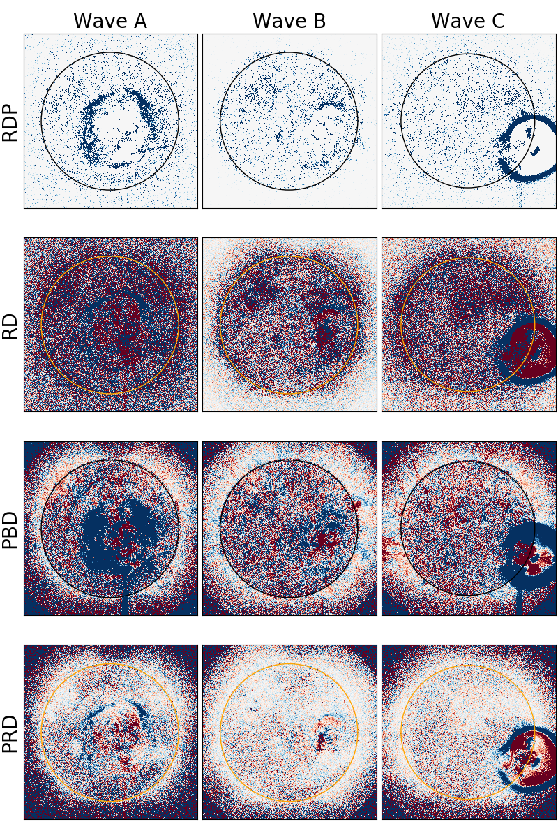
Figure 1.: Illustration of the effect of four different imaging processing techniques applied to three EUV waves. The columns show the result of applying different differencing methods to three different EUV wave events as seen in the AIA 211 Å channel. Wave A refers to data 15 February 2011 02:00:24 UT, Wave B refers to 16 February 2011 14:35:48 UT and Wave C refers to 07 June 2011 06:29:12 UT (see also Figures fig:longetal8a, fig:longetal8e and fig:longetal4 respectively). In all plots, blue pixels indicate a positive change in emission, white indicates no change in emission, and red indicates a negative change in emission. The first row shows the running difference persistence (RDP) images used by AWARE (Section sec:aware:segment:persistence), the second row shows the running difference (RD) images (used in NEMO analysis), and the third row shows the percentage base difference (PBD, used by CorPITA). The final row shows the percentage running difference (PRD) images used by Solar Demon. The color representations in the RDP and RD images are identical; values are linearly scaled in the range -100 – 100. The colors in the PBD images are linearly scaled in the range -25% – 25%. The RDP images show a cleaner separation of the propagating bright wavefront compared to the other three differencing methods.rpdm˙figure

3 The AWARE Wave Characterization Algorithm

sec:aware AWARE is implemented in two stages. In the first stage, image processing techniques are used to isolate the wavefront. These are described in Section sec:aware:segment. In the second stage, the location of the propagating wavefront is estimated and a model of the propagation is fit to the wavefront motion. These are described in Section sec:aware:dynamics.

3.1 Stage 1: Image Processing Steps to Segment the Propagating Wavefront

sec:aware:segment As was noted in Sections 1 and 2, EUV waves are difficult to detect since they are faint, extensive, and propagate over a complex background image, the solar corona. This realization has driven past attempts to enhance and detect EUV waves by making use of running difference or percentage base difference images. However, these images, while enhancing potential wavefronts, remain noisy and populated by other extraneous features (see Figure rpdm_figure). AWARE adopts a new, simple, and very promising strategy for segmenting an EUV wave wavefront from image data, running differences of persistence images (Thompson and Young, 2016).

3.1.1 Segmentation Using Running Difference Persistence Images

sec:aware:segment:persistence A persistence image is found by calculating the persistence (or running maximum) value of the emission at each pixel at all locations and times. The persistence value at time $t$ of a time series $f(t)$ is simply the maximum value reached by that pixel in the time range $0\rightarrow t$. If at later times the pixel value increases, the persistence value increases accordingly. If the pixel value decreases however, the persistence value remains unchanged. Hence, a set of persistence maps constructed from an image sequence will indicate the brightest values yet achieved in that sequence at each $t$. The persistence transform $P(t)$ of the time-series $f(t)$ is defined as

$$\ilabel{eqn:persisttransform}P(t)=\max_{t^{\prime}=0}^{t^{\prime}=t}f(t^{\prime}).$$ (1)

Figure fig:persistence illustrates the persistence transform $P(t)$ of a time-series of simulated data $f(t)$. In AWARE, the persistence transform is applied on a pixel-by-pixel basis on time-ordered sets of AIA images to obtain a persistence transform of the original AIA images. The running difference of these images generates the running difference persistence (RDP) images. Figure rpdm_figure illustrates RDP images for three example EUV wave events (these were also analyzed by CorPITA (Long et al., 2014)). The first row shows running difference persistence (RDP) images, the basic image type used by AWARE. The second row shows running difference (RD) images, the basic image type analyzed by the NEMO algorithm (Podladchikova and Berghmans, 2005). The final row shows percentage base difference (PBD) images, used by the CorPITA algorithm. Comparison with RDP images shows that in standard RD and PBD images the wavefront is more diffuse, and much coronal structure not associated with the wavefront remains in the image. RD and PBD images also have much denser noise compared to the RDP images of the same data; hence, separating the EUV wave from the noise is substantially easier when using RDP images.

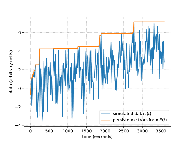
Figure 2.: Example of the application of the persistence transform. The original data $f(t)$ is shown in blue, and its persistence transform $P(t)$ is shown in red.fig:persistence

RDP images have two desirable properties when searching for EUV waves. Firstly, only pixels that brighten over previous values have a non-zero value in the running difference of persistence images, while zero-value pixels correspond to areas that did not increase in brightness. Hence, since an EUV wave brightens neighboring pixels as it moves across the Sun, the RDP images isolate those brightening pixels. In other words, the RDP images isolate the leading part of the wavefront that brightened new pixels. Secondly, since much of the corona does not vary significantly during an EUV wave, RDP images show very little residual coronal structure distant from the EUV, greatly simplifying the resulting images.

3.1.2 Reducing Noise in Running Difference Persistence Images

sec:aware:segment:noise EUV waves are faint against the background corona and so some additional steps are applied in order to improve the chance of their detection. The image processing steps used to segment the EUV wave from the input data are described below. In the following, a datacube refers to a three-dimensional array of data ordered as $(x,y,t)$, two spatial directions $(x,y)$ and one temporal direction $t$. An image is a slice in the datacube at a fixed value of time $t$.

1. Given a set of time-ordered solar EUV images (e.g. SDO/AIA or STEREO/EUVI data), data are summed in time and space to increase the signal to noise ratio of the wave against the background. Images may be summed in space as desired, for example an AIA image may be binned using $2\times 2$ super-pixels to form $2048\times 2048$ pixel images. In the time dimension, images may be summed as required. Typically, pairs or triplets of consecutive images are used. After this step the datacube consists of $N_{D}$ images (the summations in the space and time dimensions are used to determine the EUV wave detections shown in Figures fig:longetal4, fig:longetal6, fig:longetal7, fig:longetal8a, and fig:longetal8e).

2. The persistence transform is then applied to the resulting image set. This creates a set of persistence images, showing the brightest values obtained in each pixel (Equation eqn:persisttransform) as a function of time.

3. Perform a running difference operation on the persistence images. Hence, only areas that increase in brightness from one time to the next remain. An example RDP image is given in Figure method_figurea. There are now $N_{D}-1$ images in a datacube $R(x,y,t)$.

4. The dynamic range of the datacube $R(x,y,t)$ is reduced by applying a square root transformation. AWARE uses a percentile clipping on the transformed datacube where the top 1% of the intensity distribution in the datacube are clipped and set to the value at the 99%th percentile. This filters out spikes in the data caused by cosmic ray strikes, bright flares, etc. The datacube is then normalized to the range zero to 1, yielding a datacube $D(x,y,t)$. The purpose of this step is to remove the high values so that the intensity distribution better represents the bulk of the image pixels.

5. The above steps extract propagating features from the input datacube.

   However, the resulting images $I_{i}$ $(1\leq i\leq N_{D}-1)$ still show substantial noise. The following steps are intended to further isolate the wavefront by applying additional filtering steps that analyze each image at multiple length-scales $r_{k},1\leq k\leq N_{r}$.

   1. Apply a noise reduction filter to the data cube of images. Our demonstration algorithm uses a two-dimensional median filter applied to each image in the datacube. This replaces every pixel in the image with the median value found in its neighborhood. The median filter used is a circle $C_{r_{k}}$ in the spatial dimensions with a given radius $r_{k}$ pixels. The median filter is a commonly used and simple method of removing noise from an image (Gonzalez and Woods, 2001). The resulting image is $I_{noise,k}=\mbox{median}(I,C_{r_{k}})$. An example of the effect of this operation is shown in Figure method_figureb.

   2. Apply a morphological closing operation to the noise-reduced image (Gonzalez and Woods, 2001). This operation helps to close small ‘cracks’ in structures. The structuring element used is the same as that used by the median filtering operation, and generates an image $I_{close,k}=I_{noise,k}\bullet C_{r_{k}}$, where $\bullet$ denotes the morphological closing operator. An example of the effect of this operation is shown in Figure method_figurec.

6. The non-zero locations in the image $F(x,y)=\sum_{k=1}^{N_{r}}I_{close,k}(x,y)$ indicates the location of the EUV wave as determined by the multi-scale operations in the previous step. Note that the temporal summing needs to be large enough so that when the running difference of the persistence image is calculated a significant number of pixels are newly brightened in the data so that the median noise reduction at the specified length scale does not replace those pixels with zeroes (the background value).

7. Masks indicating the non-zero locations in each image $F$ are created:

   $$\mbox{mask}(x,y)=\left\{\begin{array}[]{ll}1&,F(x,y)>0\\ 0&,\mbox{otherwise}.\\ \end{array}\right.$$

The final product is a datacube of time-ordered series of $N_{D}-1$ masks $M(x,y,t)$ that localize the bright wavefront of the EUV wave. This is the AWARE stage 1 data product which is used to detect and characterize EUV wave propagation. The mask datacube is clearly time-dependent. However, the wave progress can be summarized for illustrative purposes as a static image by creating a wave progress map, defined as

$$\ilabel{e:waveprogressmap}\mbox{wave progress map}(x,y)=\left\{\begin{array}[]{ll}\max(t),&M(x,y,t)-M(x,y,t-1)>0,1\leq t\leq N_{D}-1\\ 0,&\mbox{otherwise}.\\ \end{array}\right.$$ (2)

The wave progress map summarizes the results of stage 1 of AWARE, indicating the time at which the leading edge of the wavefront is detected. Figures fig:syntheticwave:resultsa, fig:longetal4a, fig:longetal7a, fig:longetal6a, fig:longetal8aa and fig:longetal8ea show examples of wave progress maps. In the following section, the characterization of the EUV wave dynamics is described.

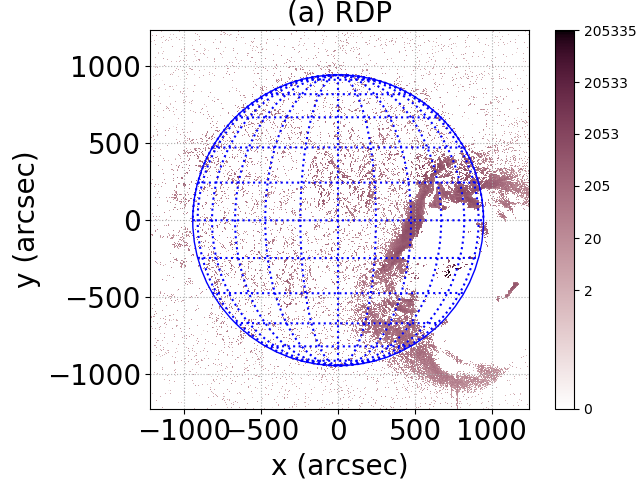
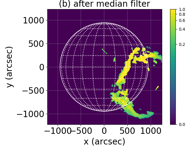
Figure 3.: (a) Shows the running difference image between two consecutive persistence images. The wavefront is already evident. (b) Shows the image at the same time after applying the median filter (Section sec:aware:segment). (c) Shows the resulting image after the morphological closing operation is applied. This has the effect of filling in small gaps in the detected wavefront (e.g. Gonzalez and Woods, 2001).method˙figure

3.2 Stage 2: Determining Wave Dynamics

sec:aware:dynamics The output of the first stage of AWARE is a time-ordered series of masks that indicate regions that were progressively brightening (summarized by wave progress maps - see Equation e:waveprogressmap, Section sec:aware:segment and Figure fig:syntheticwave:resultsa). The second stage is to determine the dynamics of the wave using the following steps.

1. Isolate the increase in intensity due to the EUV wave. This is determined by calculating $S(x,y,t)=R(x,y,t)\times M(x,y,t)$ on a pixel-by-pixel basis, i.e. the density increase caused by the wave is evaluated at the locations indicated by the mask.

2. It is known that EUV waves are associated with solar eruptive events and so this provides a candidate location and start time for the source of the wave. The candidate location is used as a source from which the wave is launched. The equivalent pixel locations in the data $S$ of arcs emanating from the source location and propagating across the sphere of the Sun following the path of great circles are used, similar to Long et al. (2014).

3. Each arc $A$ has a unique path $A(s)=(x_{s},y_{s})$ $(0\leq s\leq 1)$ which is used to extract data from $S(x_{s},y_{s},t)$ at each time $t$. This creates a two-dimensional segment of the data as a function of time and distance along the arc. At each time, the position $p(t)$ of the wavefront and an estimate of the error $e(t)$ in that position is calculated. For the results shown here,

   $$\ilabel{e:position}\mbox{position}(t)=\frac{\sum_{s=0}^{1}S(x_{s},y_{s},t)L(s)}{\sum_{s=0}^{1}S(x_{s},y_{s},t)},$$ (3)

   where $L(s)$ is the distance along the arc from the initiation point. The position of the wavefront is the weighted mean location of the wave, weighted according to the intensity of the wavefront. The error in the position is defined as the maximum width of the wavefront at time $t$, that is,

   $$\ilabel{e:error}e(t)=L(s_{max})-L(s_{min}),$$ (4)

   where $s_{max}=\max_{s}S(x_{s},y_{s},t)\neq 0$ and $s_{min}=\min_{s}S(x_{s},y_{s},t)\neq 0$. Note that at some times, an estimate of $p(t)$ or $e(t)$ cannot be made. This can happen when there is no emission at a given time along the arc. These times are eliminated from further consideration.

4. It is common to find that noise in the data $S(x,y,t)$ yields estimates of $p(t)$ that are clearly outliers compared to the general trend of other nearby points. Long et al. (2014) also encounter this issue, and describe a novel iterative algorithm for deciding which points to consider. Instead, AWARE uses the Random Sample Consensus (RANSAC) algorithm (Fischler and Bolles (1981), see also Milligan et al. (2014)) to decide which $p(t)$ can be considered inliers and which can be discarded as outliers to a possible fit. A point $p(t)$ is considered to be an inlier if the residual between a test fit and $p(t)$ is less than the median estimated error $\mbox{median}(e(t))$. The scikit-learn (Pedregosa et al., 2011) implementation of RANSAC is used, with no other changes to the default selection of choices.

5. The points that remain after steps 3, 4 and 5 are indicated on fit participation maps (an example of the fit participation map is shown in Figure fig:syntheticwave:resultsb). If more than three points $p(t)$ are found to be inliers via the RANSAC algorithm, the progress of the wave is fit with a quadratic function

   $$\ilabel{e:quad}s(t)=s+v_{0}t+0.5at^{2}.$$ (5)

   Increasing the number of samples fits and reducing noise ($e(t)$) increases the amount of information in the data, improving the fits (Byrne et al., 2013).

3.3 Adjusted CorPITA Score

ss:adjusted CorPITA (Long et al., 2014) defines a quality score, referred to here as the CorPITA score to assess how well determined is each part of the EUV wavefront. The CorPITA score is defined as

$$\ilabel{e:longscore}\mbox{CorPITA score}=100\times\left[E_{score}+D_{score}\right]/2$$ (6)

The score weights the fit quality in two parts, an existence component $E_{score}$ and a dynamic component $D_{score}$. The existence component is the fraction of time that has a measurable extent. CorPITA defines the denominator in this fraction as the number of images processed. However, it is not known a priori at what time the wave is no longer present or detectable. In AWARE, we assume that the times of the first and last detections defines the start and end of when the wave was present and detectable. The existence component measures how well AWARE captured the existence of the wave over the maximum extent of its estimated detectable range.

The dynamic component of the score is defined as

$$\ilabel{e:longscore:dynamic}D_{score}=\frac{1}{3}\left(v_{score}+a_{score}+\sigma_{score}^{rel}\right),$$ (7)

where each of the scores have value 1 if the measured value is within pre-defined limits and zero otherwise. In Long et al. (2014), if $1<v_{\mbox{fit}}<2000\,\mbox{km}\mbox{s}^{-1}$ then $v_{score}=1$ and if $-2<a_{\mbox{fit}}<2\,\mbox{km}\mbox{s}^{-2}$ then $a_{score}=1$. If the mean value of the relative error in the fit position is less than 0.5, then $\sigma_{score}^{rel}=1$. AWARE uses an adjusted version of the CorPITA score in which $v_{score}$ is defined as the integral of a normal probability distribution with mean value $v_{\mbox{fit}}$ and width equal to the error in $v_{\mbox{fit}}$, integrated between the same pre-defined limit range as Long et al. (2014). In comparison, this introduces more fit quality information to the existing CorPITA score. The quantity $a_{score}$ is defined similarly. AWARE calculates this adjusted CorPITA score for each arc.

4 Results

sec:results To test the performance of the AWARE algorithm, it is useful to analyze signals where the underlying wave properties are already known. We therefore apply AWARE to a simulated wave with known properties, and compare the detection and characterization of AWARE with the actual wave characteristics. This allows us to identify systematic errors in the analysis process.

4.1 Characterization of AWARE Using Simulated Data

ss:char The AWARE software suite contains a package that generates simulations of EUV waves propagating across the disk of the Sun. Many different parameters of the wave kinematics can be altered, such as its kinematic profile, its width, dispersion, signal to noise ratio, and origin on the solar disk. This simulation software is used to assess how well the AWARE detection and characterization software is performing (Section sec:aware). Section sss:offcenter describes a simulated wave, the application of AWARE to these simulated data, and compares the AWARE results to the known properties of the wave. Section sss:bic tests the ability of AWARE to determine if a wave is accelerating or not, and Section sss:fitbias demonstrates the existence of a systematic bias in the values of $v_{0}$ and $a$ that must be present in any algorithm (including AWARE) that allows for the wavefront to accelerate.

4.1.1 Detection and Characterization of an Example Simulated Wave

sss:offcenter A circularly propagating wave with an initial velocity $v_{\mbox{true}}=466.5\,\mbox{km}\mbox{s}^{-1}$ and acceleration $a_{\mbox{true}}=1.5\,\mbox{km}\mbox{s}^{-2}$ is launched from heliographic position $(-22\degree,-33\degree)$. The wave has a Gaussian profile in the direction of propagation, with a width of $0.49\degree$. The wave has an amplitude of 1 (in arbitrary units). The position of the wave is calculated once every 12 seconds for 60 consecutive images. Images are 1024 by 1024 pixels, with diameter of the disk the same width as the image. Noise in each image is Poisson-distributed with a mean value of 1.

AWARE is implemented on the resulting simulated dataset as follows. To increase the signal-to-noise ratio (see Section sec:aware:segment), the images are binned in to $2\times 2$ super-pixels and are pair-summed in time. Finally, the noise reduction and morphological closing operations are applied (see Section sec:aware:segment) using disks of radius $22^{\prime\prime}$. The results are shown in Figure fig:syntheticwave:results and Figure fig:syntheticwave:dynamics.

Figures fig:syntheticwave:results and fig:syntheticwave:dynamics illustrate various data products produced by AWARE. Figure fig:syntheticwave:resultsa is a wave progress map (Equation e:waveprogressmap) and shows the pixels at which wave progress is detected by stage one of AWARE (Section sec:aware:segment). Figure fig:syntheticwave:resultsb shows the fit participation map, the locations that determine the wave dynamics (found through AWARE stage 2 - see Section sec:aware:dynamics). Figure fig:syntheticwave:resultsc shows the fitted arcs and their CorPITA score. Figure fig:syntheticwave:resultsd shows the wave progress along each arc as a function of time since the initiation time. Figures fig:syntheticwave:resultse and f show the values $v_{\mbox{fit}}$ and $a_{\mbox{fit}}$ respectively and their estimated error as a function of angle around the initiation point. Figure fig:syntheticwave:resultsg shows the wave location and its error as a function of time along the arc which has the highest CorPITA score. Red lines in each of the plots (a-f) indicate the location of the arc with the highest CorPITA score. The remaining lines in Figures fig:syntheticwave:resultsa-f indicate the $0\degree,90\degree,180\degree$, and $270\degree$ longitudinal extent around the wave source.

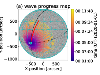
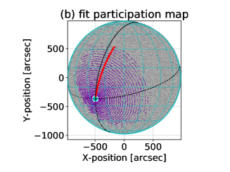
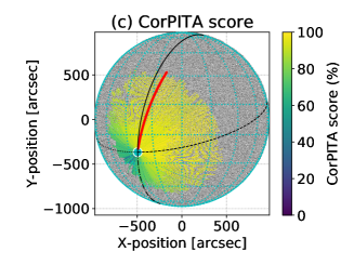
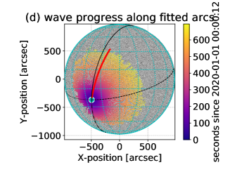
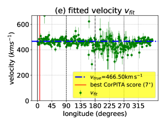
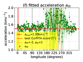
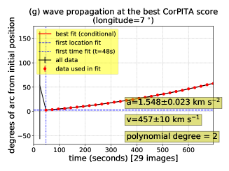
Figure 4.: AWARE applied to simulated data, a wavefront propagating evenly out from an off-disk center initiation point with an initial velocity of $466.5\,\mbox{km}\mbox{s}^{-1}$ and an acceleration of $1.5\,\mbox{km}\mbox{s}^{-2}$. (a) Is the result of stage 1 (Section sec:aware:segment), the wave progress map (Equation e:waveprogressmap). (b) Is the fit participation map showing the locations at which the wavefront is fit, and is the result of AWARE stage 2 (Section sec:aware:dynamics). (c) Is the CorPITA scorefor each of the arcs. (d) Shows the fitted arcs and the fitted wave propagation. In (a–d) the red line indicates the position and extent of the arc with the highest CorPITA score. The solid, dashed, dot-dashed and dotted black lines indicate the $0\degree,90\degree,180\degree$, and $270\degree$ angular location around the wave source. (e, f) Show the mean and standard deviation of the wavefront velocity and accelerations respectively, as a function of longitudinal angle around the source. (g) Shows the wave progress along the angle with the best CorPITA score.fig:syntheticwave:results

Figure fig:syntheticwave:dynamics shows the distributions of the dynamics of the wave detection. Figure fig:syntheticwave:dynamicsa shows a clear dependence of $v_{\mbox{fit}}$ and $a_{\mbox{fit}}$, even although the simulated wave does not include this dependence. The reasons for this dependence are explored more fully in Section sss:fitbias. Figures fig:syntheticwave:dynamicsb and c show the distribution of $v_{\mbox{fit}}$ and $a_{\mbox{fit}}$ with the CorPITA score. All plots demonstrate that although there is a spread in the values recovered compared to the true values, the mean value is correctly recovered (see also Figure fig:syntheticwave:resultse and f).

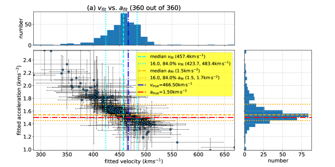
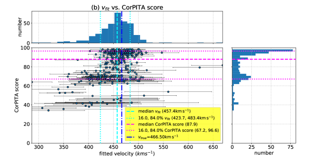
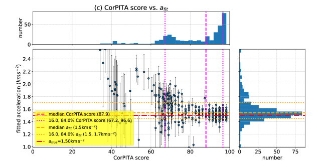
Figure 5.: Distributions of $v_{\mbox{fit}}$, $a_{\mbox{fit}}$ and the CorPITA score for the fitted arcs of the simulated data. (a) Shows $v_{\mbox{fit}}$ versus $a_{\mbox{fit}}$; median values and 16% and 84% percentile values of each quantity are shown (for normal distributions the 16% and 84% percentile values indicate the mean value plus/minus one sigma). The title of (a) shows the number of arcs fitted out of a possible 360). Error bars are the one-sigma errors reported by the fit algorithm (stage 2, step 7). (b) shows $v_{\mbox{fit}}$ versus the CorPITA score, and plot (c) shows the CorPITA score versus $a_{\mbox{fit}}$.fig:syntheticwave:dynamics

Figure fig:syntheticwave:statistics shows the average behavior of AWARE as a function of longitude around the source in recovering the true initial velocity $v_{\mbox{true}}$ and acceleration $a_{\mbox{true}}$. The mean value and standard deviation error bars are shown. These results are found by running AWARE on 100 noisy realizations of the wave setup described in Section sss:offcenter. Even with the very low signal-to-noise ratio of the simulated wave, the algorithm recovers a range of values that include the $v_{0}$ and $a$ values along all arcs, but with a substantial error. There is a small but systematic offset in the fit value of the acceleration in the range $0-180\degree$. These systematic effect is caused by projection effects in creating the simulated data, and in determining which pixels lie on arcs from the initial point. These systematic effects are more notable in the angular range $180-270\degree$ and are due to foreshortening making fewer pixels available (Figure fig:syntheticwave:results). However, the range of values indicated by the error bar suggests that the systematic offset is much less than the expected error due to noise. The error in both $v_{\mbox{fit}}$ and $a_{\mbox{fit}}$ increases in the angular range $180-270\degree$, due to the lower number of positions at which AWARE finds a propagating wave. The average value of $v_{\mbox{fit}}$ decreases here, and the average value of $a_{\mbox{fit}}$ increases, suggesting that the two quantities are not independent of each other, as was already seen in Figure fig:syntheticwave:dynamicsa. This dependence is explored further in Section sss:fitbias.

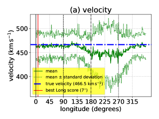
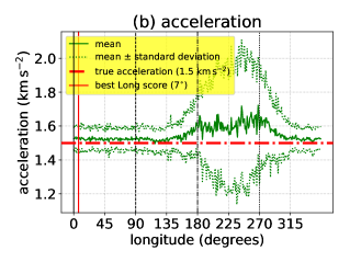
Figure 6.: (as) Scatter of recovered values of $v_{\mbox{fit}}$ and $a_{\mbox{fit}}$ (b) for 100 runs of AWARE on different noisy versions of the simulated wave.fig:syntheticwave:statistics

4.1.2 Velocity-Acceleration Correlation as a Source of Bias

sss:fitbias The error in determining the position of the wave is a significant source of error in determining the errors in $v_{\mbox{fit}}$ and $a_{\mbox{fit}}$. Figure f:biased_fittinga–d shows the scatter in the fit initial velocity and acceleration found in 10000 noisy realizations of a test arc. The plots show that fitting any particular realization of the true wave progress can lead to velocities and accelerations that are very distant from $v_{\mbox{true}}$ and $a_{\mbox{true}}$. It is easy to see how the correlation between the fit velocity and acceleration arises by considering Equation e:quad and the fitting process. The fitting process calculates

$$D=\min\sum_{i=1}^{n_{t}}\left[\frac{s(t_{i})-p(t_{i})}{e(t_{i})}\right]^{2}\ilabel{e:min}$$ (8)

by varying the values of $a_{0}$ and $v_{0}$. If the fit finds a value of $a_{0}$ that is a higher than the true value then a lower value of $v_{0}$ is preferred for the minimization. Similarly, if the fit finds a value of $a_{0}$ that is lower than the true value then a higher value of $v_{0}$ is sought by the minimization routine. This leads to correlated values of $a_{\mbox{fit}}$ and $v_{\mbox{fit}}$.

It is also notable that the histograms shown in the top and bottom rows of Figure f:biased_fitting illustrate different scattering behavior around the true values. This is due to the number of samples in each time series. For smaller numbers of samples, there is less information to constrain fit values, and so the scatter about the true value increases. Increasing the number of samples not only reduces the scatter but changes the $a_{\mbox{fit}}$, $v_{\mbox{fit}}$ correlation. With more information, a small change in the value of $a_{0}$ means that the fit requires a bigger change in the value of $v_{0}$ in order to reach a minimum. This can be understood by considering Equation e:min for two different fits. Assume there is a fit $s(t)=S+Vt+At^{2}/2$ giving a value $D$; now perturb that fit and consider $s^{\prime}(t)=(S+s)+(V+v)t+(A+a)t^{2}/2$ (for simplicity we also assume that $e(t_{i})$ is 1 for all $t_{i}$) giving a value $D^{\prime}$. If we assume that $D\approx D^{\prime}$ (both fits give approximately the same value), and consider each summand in Equation e:min then

e:bias$$v \approx \frac{-at^{4}\left(2A+a\right)/4-Vat^{3}+t^{2}\left(As+Sa+as+v^{2}-ay\right)-2Vst-2Ss-s^{2}+2sy}{t^{3}\left(A+a\right)+2Vt^{2}+2t\left(S+s-y\right)}$$ (9)

$$\rightarrow -\frac{a}{4}\left(\frac{2A+a}{A+a}\right)t$$

as $t\rightarrow\infty$. Hence as larger times are considered, small changes in the acceleration inevitably lead to larger changes in the velocity to achieve the same quality of fit. Equation e:bias also explains the negative correlation between the fit velocity and acceleration.

Figure f:biased_fittinge is generated by creating 200 simulated wavefront propagation profiles with random properties and using the fit process described in Section sec:aware:dynamics to derive values of $v_{\mbox{fit}}$ and $a_{\mbox{fit}}$. The number of samples in each profile is drawn from $U_{integer}(10,60)$ , and the true initial velocity is drawn from $U(0,1000)$and the true initial acceleration is drawn from $U(-1,1)$. Plotting $v_{\mbox{fit}}$ against $a_{\mbox{fit}}$ shows an apparent correlation, even although the true values are uncorrelated since they are drawn from independent uniform distributions. This complicates the discussion of Long et al. (2017a) as to if there is true, physical correlation between the initial velocity and the acceleration. One way of estimating if there is a true physical correlation is to fit multiple noisy realizations of the original data to generate a probability distribution $P(\rho)$ of correlation coefficients and then compare that distribution to the correlation coefficient $\rho_{o}$ derived from the original velocity versus acceleration scatter. If the complementary cumulative probability value $1-\int_{-\infty}^{\rho_{o}}P(\rho^{\prime})d\rho^{\prime}$ is close to zero then it is very unlikely that the correlation value $\rho_{o}$ arose by chance, lending support that the initial velocity and acceleration are indeed correlated.

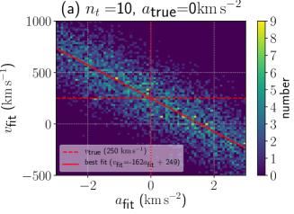
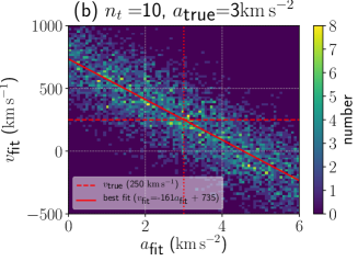
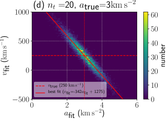
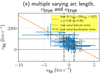
Figure 7.: (a–d) Shows two dimensional histograms of the $v_{\mbox{fit}}$ and $a_{\mbox{fit}}$ correlation. The histograms of $v_{\mbox{fit}}$ and $a_{\mbox{fit}}$ are found by fitting a quadratic polynomial to 10000 noisy realizations of one arc in a wavefront. All plots were generated assuming a 5 degree error in locating the wavefront. (a, c) Shows results with $a_{\mbox{true}}=0\,\mbox{km}\mbox{s}^{-2}$. (b, d) shows results with $a_{\mbox{true}}=3\,\mbox{km}\mbox{s}^{-2}$. Comparing (a, b) to (c, d) shows that the $a_{\mbox{fit}},v_{\mbox{fit}}$ dependency is a function of the number of samples in the time-series $n_{t}$ (sample cadence is 36 seconds for all plots). It is clear that there is a dependency between $a_{\mbox{fit}}$ and $v_{\mbox{fit}}$ and that the number of samples in the time series varies the dependence. The solid red line in the plot indicates the line of best fit assuming a linear dependence of $v_{\mbox{fit}}$ on $a_{\mbox{fit}}$. (e) Shows how it is possible to create a correlation even when each arc has a different initial velocity, initial acceleration and number of samples $n_{t}$. See Section sss:fitbias for more details.f:biased˙fitting

4.1.3 Detection of Accelerating Versus Non-Accelerating Wavefronts

sss:bic

Figure 8.: The effect of the degree of the polynomial used to fit a simulated wave arc as a function of the wave acceleration. The x-axis indicates the true value of the acceleration in the simulated wavefront. (a) Shows the median and median absolute deviation velocity derived from fitting either a $n=1$ or an $n=2$ polynomial. (b) Shows the median and median absolute deviation acceleration derived from fitting a $n=2$ polynomial (the red true acceleration line is fully covered by the blue line indicating the value derived from fitting). (c) Shows the median and median absolute deviation difference in the Bayesian information criterion (BIC) calculated from each polynomial fit. Positive values indicate that the BIC correctly prefers the $n=2$ polynomial fit containing an acceleration term. (note that BIC₁ refers to the BIC value for the $n=1$ model, and BIC₂ refers to the BIC $n=2$ value model). The degree of preference for each model ($n=1$ or $n=2$) is indicated on the left hand side of the plot (Kass and Raftery, 1995). The simulation assumed that the position of the wavefront was measured at 20 times, with a cadence of 36 seconds between each measurement. The wave position had a normally distributed error of 5 degrees of arc. The propagation of the wavefront along the arc was simulated 1000 times to generate the results.fig:acc˙versus˙non˙acc

One test for the existence of accelerating wavefronts is to fit linear ($n=1$) or quadratic ($n=2$) functions to the progress of the wave along each arc, and then decide which fit is a reasonable explanation for the data. For illustrative purposes, we use the Bayesian information criterion (BIC) (Schwarz, 1978) to perform model selection, in this case, to decide between the linear and quadratic fits to the arc progress. The BIC is defined as

$$BIC=-2\ln(L)+k\ln(N),\ilabel{eqn:bic}$$ (10)

where $L$ is the likelihood function evaluated at its maximum, $k$ is the number of parameters in the fitting function, and $N$ is the number of values fit. Since we are assuming that the location of the wavefront is Gaussian-noisily distributed, maximizing the likelihood function is equivalent to the least squares fit used in AWARE to fit either linear or quadratic functions to the data. The model with the lowest BIC is the preferred model.

Figure fig:acc_versus_non_acca shows the fit initial velocity $v_{\mbox{fit}}$ derived from fitting the simulated wavefront using linear and quadratic functions. As expected, the linear function performs poorly except close to $a_{\mbox{true}}=0$. Away from $a_{\mbox{true}}=0$, the linear function is attempting to compensate for the accelerating progress of the wave by changing the initial velocity, leading to initial velocities with magnitudes much larger than the true value of $v_{0}$. Figure fig:acc_versus_non_accb shows that the quadratic fit recovers the true acceleration with a relatively small error. Figure fig:acc_versus_non_acc c shows the difference in the BIC for each model. Positive values indicate a preference for the correct model $n=2$ which includes an acceleration. Negative values indicate a preference for the linear model. The degree of preference is also indicated by the different colored regions, following the classification of Kass and Raftery (1995). The plot shows that the accelerating model is not strongly preferred until the magnitude of the acceleration is around $2\,\mbox{km}\mbox{s}^{-2}$. Therefore at lower magnitude accelerations, fits with and without accelerations are not easily distinguishable.

4.2 Application to Observational Data

sec:obs The AWARE algorithm is applied to datasets derived from the results shown in the CorPITA article (Long et al., 2014), the EUV waves of 7 June 2011 (Figure fig:longetal4, 13 February 2011 (Figure fig:longetal7), 15 February 2011 (Figure fig:longetal8a), and 16 February 2011 (Figure fig:longetal8e). The algorithm is also applied to the same time range analyzed by (Long et al., 2014) from 8 February 2011 (Figure fig:longetal6) to illustrate a null result. In all cases, full spatial resolution FITS level 1.0 AIA 211 Å image data at 12 second cadence in the hour following the initiating eruptive event are downloaded and analyzed.

The wave progress maps (Figures fig:longetal4a, fig:longetal6a, fig:longetal7a, fig:longetal8aa, and fig:longetal8ea) illustrate the initial identification of the wave location. It is notable that the algorithm captures changes that are quite distant from the wave source at earlier times. These are clearly unphysical, as the wave cannot have reached those locations so soon after its initiation. These initial wave progress locations are obtained from stage 1 of the algorithm. At these earlier times, small changes at distant locations are captured by the RDP image processing and expanded into contiguous areas by the morphological processing. The effect of this is mitigated somewhat by stage 2 of the algorithm (fitting a profile to the wave propagation along radial arcs beginning at the initiation point) where the mean location of the wavefront and its error often lead to the elimination of earlier times from consideration in the final fit.

It is difficult to exactly compare the AWARE results to the results of Long et al. (2014). The wave progress maps (Figures fig:longetal4a, fig:longetal6a, fig:longetal7a, fig:longetal8aa, and fig:longetal8ea) are broadly similar to the wave pulse propagation maps of Long et al. (2014) (although it may be more appropriate to compare the fitted arcs maps of Figures fig:longetal4d, fig:longetal6d, fig:longetal7d, fig:longetal8ad, and fig:longetal8ed). The locations of fitted wave propagation found are broadly similar, but without doing an actual numerical comparison, it is difficult to accurately assess if the AWARE maps show more successfully fitted arcs than any other algorithm. Reassuringly, running AWARE on the null result data suggested by Long et al. (2014) and shown here in Figure fig:longetal6 produces a similar null result. The values of $a_{\mbox{fit}}$ and $v_{\mbox{fit}}$ found (Figures fig:longetal4e and f, fig:longetal4dynamics, fig:longetal7e and f, fig:longetal7dynamics, fig:longetal8ae and f, fig:longetal8adynamics, fig:longetal8ee and f, fig:longetal8edynamics) for all EUV waves appear reasonable compared to the values obtained in the literature. Firstly, Long et al. (2014) in analyzing the 15 February 2011 event (their Figure 8a – d, Figures fig:longetal8a and fig:longetal8adynamics here), CorPITA returned an average $v_{\mbox{fit}}$ of $406\pm 1\,\mbox{km}\mbox{s}^{-1}$ in the range $0\rightarrow 1000\,\mbox{km}\mbox{s}^{-1}$. Calculating over all the measured arcs, AWARE returns a mean $v_{\mbox{fit}}$ value of $584\pm 258\,\mbox{km}\mbox{s}^{-1}$, a median value of $551\,\mbox{km}\mbox{s}^{-1}$, a central 68% width $199\rightarrow 877\,\mbox{km}\mbox{s}^{-1}$, with all values falling in the range of $0\rightarrow 1200\,\mbox{km}\mbox{s}^{-1}$ approximately. For the 16 February 2011 event, Long et al. (2014) quote an average $v_{\mbox{fit}}$ of $331\pm 6\,\mbox{km}\mbox{s}^{-1}$ in a range varying $\approx 100\rightarrow 975\,\mbox{km}\mbox{s}^{-1}$(their Figure 8e – h, Figures fig:longetal8e and fig:longetal8edynamics here). AWARE returns a mean $v_{\mbox{fit}}$ value of $592\pm 453\,\mbox{km}\mbox{s}^{-1}$ (over all arcs), a median $v_{\mbox{fit}}$ value of $442\,\mbox{km}\mbox{s}^{-1}$, a central 68% width of $13\rightarrow 820\,\mbox{km}\mbox{s}^{-1}$, with all values falling in the range of $0\rightarrow 2000\,\mbox{km}\mbox{s}^{-1}$ approximately. Although these values are not the same, they are comparable in magnitude. Secondly, Long et al. (2017a) applied the CorPITA algorithm to 362 EUV events originally identified by Nitta et al. (2013). Median values to the spread of velocities and accelerations found in each event are quoted; CorPITA finds median velocities in the range of $0\rightarrow 950\,\mbox{km}\mbox{s}^{-1}$ and median accelerations in the range of $-0.75\rightarrow 0.1\,\mbox{km}\mbox{s}^{-2}$ Nitta et al. (2013) quote a velocity range of $200\rightarrow 1400\,\mbox{km}\mbox{s}^{-1}$, and an acceleration range of $-0.7\rightarrow 0.3\,\mbox{km}\mbox{s}^{-2}$. For the events analyzed here, AWARE finds a range of velocities $0\rightarrow 2000\,\mbox{km}\mbox{s}^{-1}$, and accelerations in the approximate range of $-1.7\rightarrow 1.9\,\mbox{km}\mbox{s}^{-2}$, overlapping with the results of Long et al. (2017a) and Nitta et al. (2013). All detections show a correlation between $a_{\mbox{fit}}$ and $v_{\mbox{fit}}$. Figure fig:longetal8adynamicsa differs from similar plots in that there appears to be two separate branches of $a_{\mbox{fit}}$ and $v_{\mbox{fit}}$ dependence above the median value of $v_{\mbox{fit}}$. Interpreting this using the discussion of Section sss:fitbias suggests weak evidence for either two different distinctive durations of the wavefront or that the ratios of $v_{\mbox{true}}/a_{\mbox{true}}$ differ significantly in at least two locations. Given that the CorPITA score values (Figure fig:longetal8adynamicsb, c) do not show evidence of two populations (which could be caused by having two populations that have a significant difference in their duration, as measured by the existence component $E_{score}$ in Equation e:longscore) then this suggests an interpretation in terms of differing $v_{\mbox{true}}/a_{\mbox{true}}$ ratios.

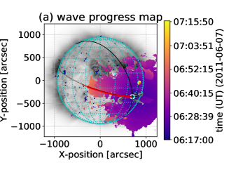
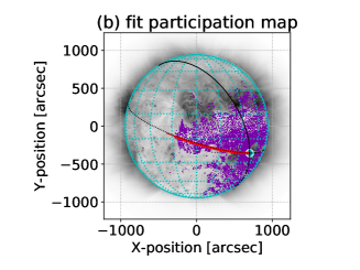
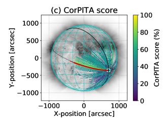
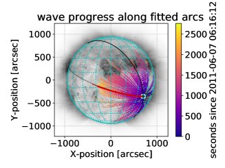
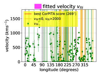
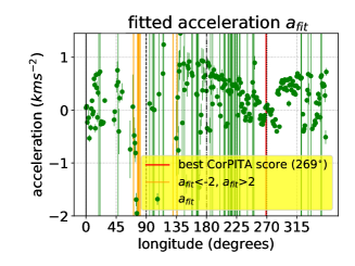
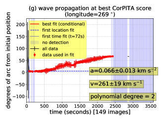
Figure 9.: AWARE performance for the EUV wave of 7 June 2011. See the caption of Figure fig:syntheticwave:results for more details.fig:longetal4

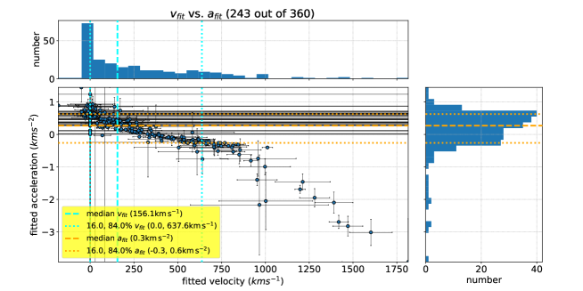
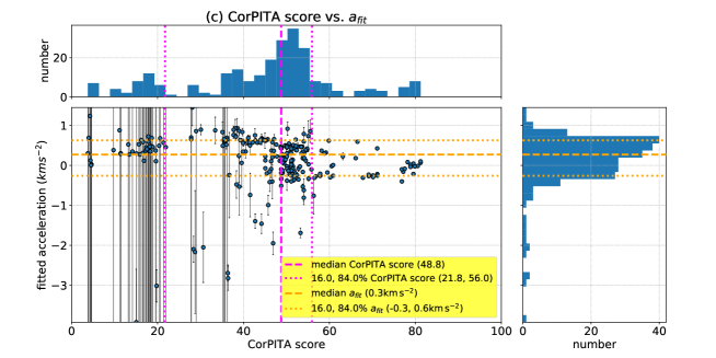
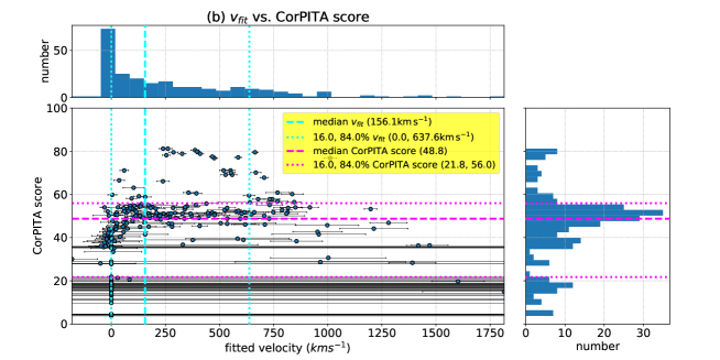
Figure 10.: Distributions of $v_{\mbox{fit}}$, $a_{\mbox{fit}}$, and the CorPITA score for the fitted arcs of the 7 June 2011 EUV wave. See the caption of Figure fig:syntheticwave:dynamics for more details.fig:longetal4dynamics

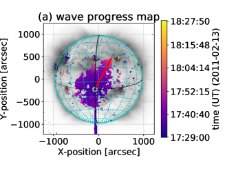
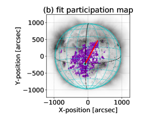
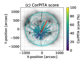
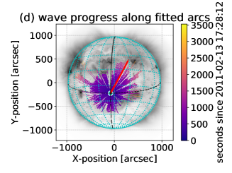
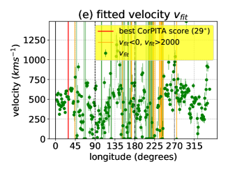
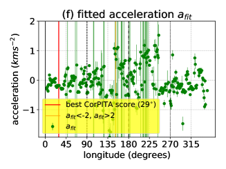
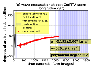
Figure 11.: AWARE performance for the EUV wave of 13 February 2011. see the caption of Figure fig:syntheticwave:results for more details.fig:longetal7

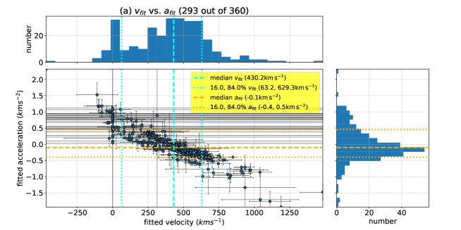
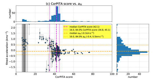
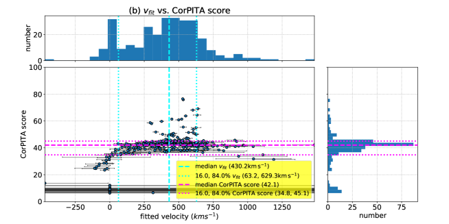
Figure 12.: Distributions of $v_{\mbox{fit}}$, $a_{\mbox{fit}}$ and the CorPITA score for the fitted arcs of the 13 February 2011 EUV wave (see Figure fig:longetal7). See the caption of Figure fig:syntheticwave:dynamics for more details.fig:longetal7dynamics

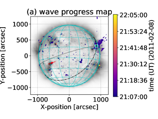
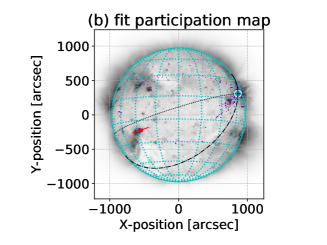
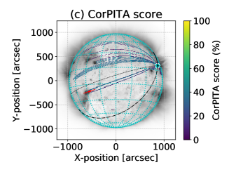
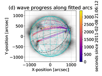
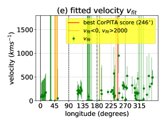
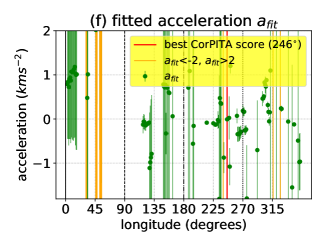
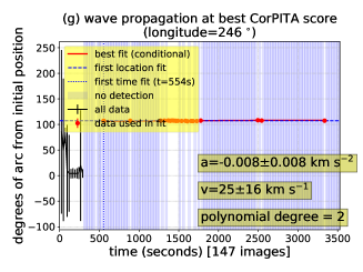
Figure 13.: AWARE performance when there is no EUV wave identifiable by eye, using the same data analyzed by Long et al. (2014) and shown in their Figure 6. See the caption of Figure fig:syntheticwave:results for more details.fig:longetal6

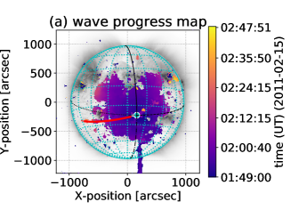
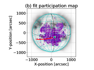
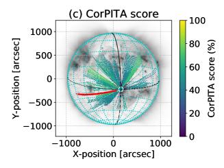
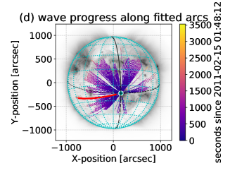
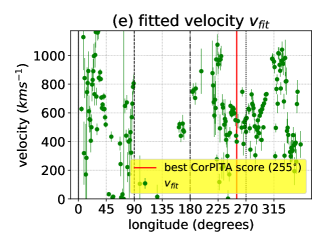
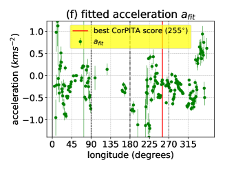
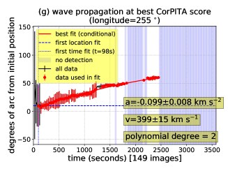
Figure 14.: AWARE performance for the EUV wave of 15 February 2011. See the caption of Figure fig:syntheticwave:results for more details.fig:longetal8a

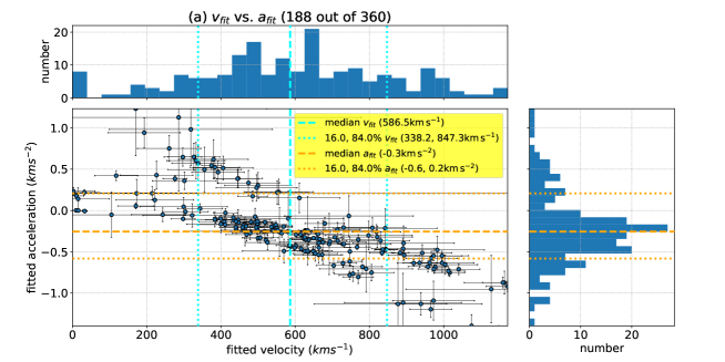
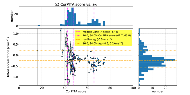
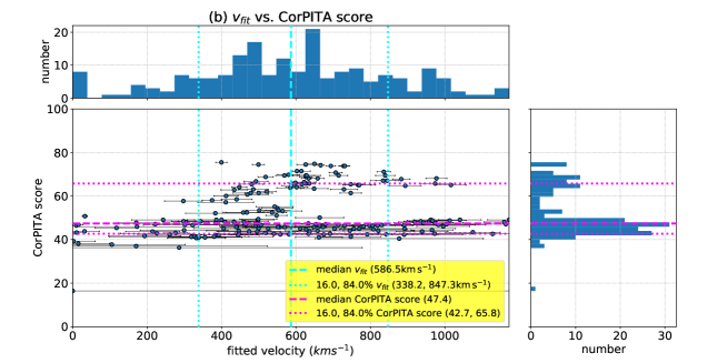
Figure 15.: Distributions of $v_{\mbox{fit}}$, $a_{\mbox{fit}}$ and the CorPITA score for the fitted arcs of the 15 February 2011 EUV wave (see Figure fig:longetal8a). See the caption of Figure fig:syntheticwave:dynamics for more details.fig:longetal8adynamics

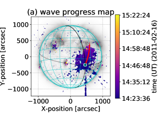
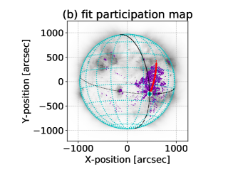
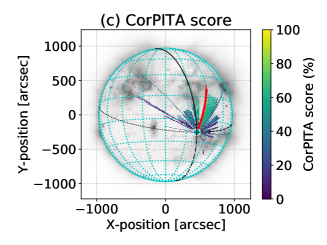
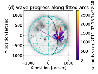
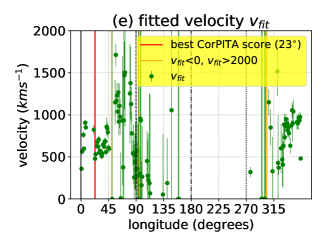
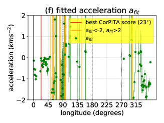
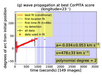
Figure 16.: AWARE performance for the EUV wave of 16 February 2011. See the caption of Figure fig:syntheticwave:results for more details.fig:longetal8e

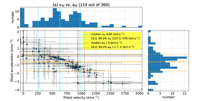
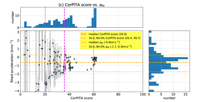
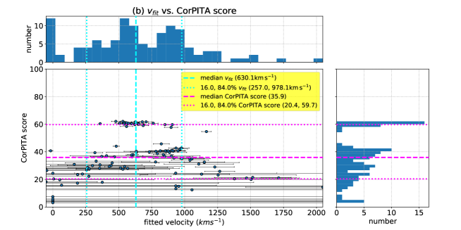
Figure 17.: Distributions of $v_{\mbox{fit}}$, $a_{\mbox{fit}}$ and the CorPITA score for the fitted arcs of the 15 February 2011 EUV wave (see Figure fig:longetal8a). See the caption of Figure fig:syntheticwave:dynamics for more details.fig:longetal8edynamics

5 Summary and Future Work

s:conclusions AWARE uses the novel running difference persistence images to isolate faint, propagating bright features in coronal channel AIA data. The algorithm then applies noise removal and morphological image operations to better isolate the wave structure. Great arcs are traced from the suspected wave launch location and the RANSAC method is used to find when and where the propagating wavefront intensity approximately fits an accelerating profile. These points are fit using a least-squares fitting algorithm to find value and error estimates of the initial velocity and acceleration of the wave. As noted above, one hour’s worth of AIA 211 Å data are used to determine the wave location and dynamics. The only criterion for determining the time-range of data to be downloaded is that it be long enough to include the possible lifetime of the wave. Stages 1 and 2 of AWARE are sufficient to estimate the wave lifetime within the time-range of data downloaded. Stage 1 of AWARE isolates propagating fronts that brighten emission as they propagate; therefore, if they are not present they will not be available for characterization in stage 2. In stage 2, the wave location as a function of time along each arc is determined. The RANSAC algorithm is used to find the inlier wave locations that satisfy the proximity criteria (see Section sec:aware:dynamics), eliminating outliers that can cause bad fits.

AWARE has been tested on both simulated and real datasets, and was found to perform well and produce results comparable with other established methods. The AWARE code repository comes with codes to generate simulated waves. The mean behavior of AWARE shows that the initial velocity and acceleration of simulated EUV waves can be recovered, subject to error. Fitting the simulated waves also demonstrates that the fitting algorithm introduces a systematic negative correlation between the fit value of the initial velocity and the acceleration. A negative correlation persists even when a diverse population of simulated wavefront propagations are considered (Section sss:fitbias). Therefore, the inherent correlation between the initial fit velocity and the acceleration must be taken into account when attempting to determine which physical mechanism is operating that creates EUV waves.

Several future refinements are possible that will improve AWARE and maximize its effectiveness and use to the solar community. On comparing the wave progress plots (Section sec:aware:segment:persistence) to the fitted wave progress plots in Figures fig:longetal4, fig:longetal7, fig:longetal8a, and fig:longetal8e, it seems clear that AWARE loses information about the wavefront. AWARE assumes purely radial propagation; future versions of AWARE could use the wave propagation maps to derive the propagation instead of assuming a radial propagation. For example, the Huygens principle method employed by Wills-Davey and Thompson (1999) and Wills-Davey (2006) captured non-radial propagation allowing the determination of wavefront curvature, variable speed, and acceleration. The analysis of Section sss:fitbias shows that reducing the error in locating the wave is crucial to improving knowledge of wave kinematics. The noise removal algorithm used in this article sums the results of the median filter applied at multiple length-scales. However, there are a number of other noise removal algorithms. For example, Gonzalez and Woods (2001) describe an adaptive median filter algorithm that varies the size scale of the area over which the median is calculated based on local greyscale values in the image. Two-dimensional wavelets, along with thresholding algorithms could be used to determine global (or local) noise levels, segmenting the wavefront from the data. Improved wave segmentation leading to smaller errors on the position of the wavefront would greatly improve our knowledge of the kinematics of EUV waves.

An operational version of AWARE will monitor the Heliophysics Event Knowledgebase (HEK) event database for new events in event types such as as solar flares and eruptions. The appearance of a new event of one of these types will trigger subsequent data download and analysis. The HEK event information will be used to determine parameters of the analysis, such as start time of the interval to be analyzed, and potential locations on the Sun of a wave origin. AWARE will perform the image processing and wave assessment steps described above, finally writing a record into a database that is easily accessed through existing solar feature and event databases. The availability of such a catalog will allow large-scale statistical studies of EUV waves and their properties. There are several additional properties that could be stored about each EUV wave in such a catalog. The total number of degrees around the starting point at which a propagating wavefront was fit would give an assessment of its total angular extent. For example, if $\theta_{wave}=360$, then there was a successful detection of the wave completely encircling the starting point. Also, the number of distinct angular regions of wave propagation would yield information as to how discontinuous the wavefront is compared to a single wave. Median values of populations are less sensitive to outliers and so the median CorPITA score of all the arcs extending from the starting point would give a useful assessment of the entire wave.

AWARE is the fourth published EUV wave detection algorithm at the time of writing. Along with NEMO, CorPITA and Solar Demon, EUV wave detection is now at the stage that it should now be possible to compare the effectiveness of these algorithms on the same simulated and observational data with the goal of obtaining useful insight on the performance of each of them (at the very least making the comparisons in Section sec:obs easier). Such comparison work has been useful in understanding the performance of automated loop tracing algorithms (Aschwanden et al., 2008) and magnetic field extrapolation (Schrijver et al., 2006; Metcalf et al., 2008). Approaches similar in style to these works would create a useful benchmark, and guide the development of improved algorithms to better determine the dynamics, and ultimately the physics, of EUV waves in the solar atmosphere.

Acknowledgments

We are grateful to the developers of SSWIDL (Freeland and Bentley, 2000), IPython (Pérez and Granger, 2007), SunPy (SunPy Community et al., 2015), matplotlib (Hunter, 2007), Scikit-Learn (Pedregosa et al., 2011), SymPy (Meurer et al., 2017) and the Scientific Python stack for providing data preparation, manipulation, analysis, and display packages. LH and JI acknowledge the support of the Solar Data Analysis Center (SDAC) through the SESDA grant 80GSFC17C0003.

References

- Aschwanden et al. (2008) Aschwanden, M.J., Lee, J.K., Gary, G.A., Smith, M., Inhester, B.: 2008, Comparison of Five Numerical Codes for Automated Tracing of Coronal Loops. Sol. Phys. 248, 359. DOI. ADS.
- Attrill et al. (2007a) Attrill, G.D.R., Harra, L.K., van Driel-Gesztelyi, L., Démoulin, P., Wülser, J.-P.: 2007a, Coronal “wave”: A signature of the mechanism making CMEs large-scale in the low corona? Astron. Nach. 328, 760. DOI. ADS.
- Attrill et al. (2007b) Attrill, G.D.R., Harra, L.K., van Driel-Gesztelyi, L., Démoulin, P.: 2007b, Coronal “Wave”: Magnetic Footprint of a Coronal Mass Ejection? ApJ 656, L101. DOI. ADS.
- Biesecker et al. (2002) Biesecker, D.A., Myers, D.C., Thompson, B.J., Hammer, D.M., Vourlidas, A.: 2002, Solar Phenomena Associated with “EIT Waves”. ApJ 569, 1009. DOI. ADS.
- Byrne et al. (2013) Byrne, J.P., Long, D.M., Gallagher, P.T., Bloomfield, D.S., Maloney, S.A., McAteer, R.T.J., Morgan, H., Habbal, S.R.: 2013, Improved methods for determining the kinematics of coronal mass ejections and coronal waves. A&A 557, A96. DOI. ADS.
- Chen (2006) Chen, P.F.: 2006, The Relation between EIT Waves and Solar Flares. ApJ 641, L153. DOI. ADS.
- Chen, Fang, and Shibata (2005) Chen, P.F., Fang, C., Shibata, K.: 2005, A Full View of EIT Waves. ApJ 622, 1202. DOI. ADS.
- Chen et al. (2002) Chen, P.F., Wu, S.T., Shibata, K., Fang, C.: 2002, Evidence of EIT and Moreton Waves in Numerical Simulations. ApJ 572, L99. DOI. ADS.
- Cohen et al. (2009) Cohen, O., Attrill, G.D.R., Manchester, W.B. IV, Wills-Davey, M.J.: 2009, Numerical Simulation of an EUV Coronal Wave Based on the 2009 February 13 CME Event Observed by STEREO. ApJ 705, 587. DOI. ADS.
- Delannée (2000) Delannée, C.: 2000, Another View of the EIT Wave Phenomenon. ApJ 545, 512. DOI. ADS.
- Delannée and Aulanier (1999) Delannée, C., Aulanier, G.: 1999, CME Associated with Transequatorial Loops and a Bald Patch Flare. Sol. Phys. 190, 107. DOI. ADS.
- Delannée et al. (2008) Delannée, C., Török, T., Aulanier, G., Hochedez, J.-F.: 2008, A New Model for Propagating Parts of EIT Waves: A Current Shell in a CME. Sol. Phys. 247, 123. DOI. ADS.
- Fischler and Bolles (1981) Fischler, M.A., Bolles, R.C.: 1981, Random sample consensus: A paradigm for model fitting with applications to image analysis and automated cartography. Commun. ACM 24(6), 381. DOI. http://doi.acm.org/10.1145/358669.358692.
- Freeland and Bentley (2000) Freeland, S., Bentley, R.: 2000, In: Murdin, P. (ed.) SolarSoft. DOI. ADS.
- Gallagher and Long (2011) Gallagher, P.T., Long, D.M.: 2011, Large-scale Bright Fronts in the Solar Corona: A Review of ”EIT waves”. Space Sci. Rev. 158, 365. DOI. ADS.
- Gonzalez and Woods (2001) Gonzalez, R.C., Woods, R.E.: 2001, Digital Image Processing, 2nd edn. Addison-Wesley Longman Publishing Co., Inc., Boston, MA, USA. ISBN 0201180758.
- Gopalswamy et al. (2009) Gopalswamy, N., Yashiro, S., Temmer, M., Davila, J., Thompson, W.T., Jones, S., McAteer, R.T.J., Wuelser, J.-P., Freeland, S., Howard, R.A.: 2009, EUV Wave Reflection from a Coronal Hole. ApJ 691, L123. DOI. ADS.
- Hunter (2007) Hunter, J.D.: 2007, Matplotlib: A 2d graphics environment. Comp.Scien. & Eng. 9(3), 90.
- Kass and Raftery (1995) Kass, R.E., Raftery, A.E.: 1995, Bayes factors. J. Am. Stat. Assoc. 90, 773.
- Kraaikamp and Verbeeck (2015) Kraaikamp, E., Verbeeck, C.: 2015, Solar Demon - an approach to detecting flares, dimmings, and EUV waves on SDO/AIA images. J. Space Weather Spac. Clim. 5(27), A18. DOI. ADS.
- Kwon et al. (2013) Kwon, R.-Y., Ofman, L., Olmedo, O., Kramar, M., Davila, J.M., Thompson, B.J., Cho, K.-S.: 2013, STEREO Observations of Fast Magnetosonic Waves in the Extended Solar Corona Associated with EIT/EUV Waves. ApJ 766, 55. DOI. ADS.
- Liu and Ofman (2014) Liu, W., Ofman, L.: 2014, Advances in Observing Various Coronal EUV Waves in the SDO Era and Their Seismological Applications (Invited Review). Sol. Phys. 289, 3233. DOI. ADS.
- Liu et al. (2012) Liu, W., Ofman, L., Nitta, N.V., Aschwanden, M.J., Schrijver, C.J., Title, A.M., Tarbell, T.D.: 2012, Quasi-periodic Fast-mode Wave Trains within a Global EUV Wave and Sequential Transverse Oscillations Detected by SDO/AIA. ApJ 753, 52. DOI. ADS.
- Long, DeLuca, and Gallagher (2011) Long, D.M., DeLuca, E.E., Gallagher, P.T.: 2011, The Wave Properties of Coronal Bright Fronts Observed Using SDO/AIA. ApJ 741, L21. DOI. ADS.
- Long et al. (2008) Long, D.M., Gallagher, P.T., McAteer, R.T.J., Bloomfield, D.S.: 2008, The Kinematics of a Globally Propagating Disturbance in the Solar Corona. ApJ 680, L81. DOI. ADS.
- Long et al. (2014) Long, D.M., Bloomfield, D.S., Gallagher, P.T., Pérez-Suárez, D.: 2014, CorPITA: An Automated Algorithm for the Identification and Analysis of Coronal ”EIT Waves”. Sol. Phys. 289, 3279. DOI. ADS.
- Long et al. (2017a) Long, D.M., Murphy, P., Graham, G., Carley, E.P., Pérez-Suárez, D.: 2017a, A Statistical Analysis of the Solar Phenomena Associated with Global EUV Waves. Sol. Phys. 292, 185. DOI. ADS.
- Long et al. (2017b) Long, D.M., Bloomfield, D.S., Chen, P.F., Downs, C., Gallagher, P.T., Kwon, R.-Y., Vanninathan, K., Veronig, A.M., Vourlidas, A., Vršnak, B., Warmuth, A., Žic, T.: 2017b, Understanding the Physical Nature of Coronal “EIT Waves”. Sol. Phys. 292, 7. DOI. ADS.
- Metcalf et al. (2008) Metcalf, T.R., De Rosa, M.L., Schrijver, C.J., Barnes, G., van Ballegooijen, A.A., Wiegelmann, T., Wheatland, M.S., Valori, G., McTtiernan, J.M.: 2008, Nonlinear Force-Free Modeling of Coronal Magnetic Fields. II. Modeling a Filament Arcade and Simulated Chromospheric and Photospheric Vector Fields. Sol. Phys. 247, 269. DOI. ADS.
- Meurer et al. (2017) Meurer, A., Smith, C.P., Paprocki, M., Čertík, O., Kirpichev, S.B., Rocklin, M., Kumar, A., Ivanov, S., Moore, J.K., Singh, S., Rathnayake, T., Vig, S., Granger, B.E., Muller, R.P., Bonazzi, F., Gupta, H., Vats, S., Johansson, F., Pedregosa, F., Curry, M.J., Terrel, A.R., Roučka, v., Saboo, A., Fernando, I., Kulal, S., Cimrman, R., Scopatz, A.: 2017, Sympy: symbolic computing in python. PeerJ Comp. Scien. 3, e103. DOI. https://doi.org/10.7717/peerj-cs.103.
- Milligan et al. (2014) Milligan, R.O., Kerr, G.S., Dennis, B.R., Hudson, H.S., Fletcher, L., Allred, J.C., Chamberlin, P.C., Ireland, J., Mathioudakis, M., Keenan, F.P.: 2014, The Radiated Energy Budget of Chromospheric Plasma in a Major Solar Flare Deduced from Multi-wavelength Observations. ApJ 793, 70. DOI. ADS.
- Moses et al. (1997) Moses, D., Clette, F., Delaboudinière, J.-P., Artzner, G.E., Bougnet, M., Brunaud, J., Carabetian, C., Gabriel, A.H., Hochedez, J.F., Millier, F., Song, X.Y., Au, B., Dere, K.P., Howard, R.A., Kreplin, R., Michels, D.J., Defise, J.M., Jamar, C., Rochus, P., Chauvineau, J.P., Marioge, J.P., Catura, R.C., Lemen, J.R., Shing, L., Stern, R.A., Gurman, J.B., Neupert, W.M., Newmark, J., Thompson, B., Maucherat, A., Portier-Fozzani, F., Berghmans, D., Cugnon, P., van Dessel, E.L., Gabryl, J.R.: 1997, EIT Observations of the Extreme Ultraviolet Sun. Sol. Phys. 175, 571. DOI. ADS.
- Nakariakov and Verwichte (2005) Nakariakov, V.M., Verwichte, E.: 2005, Coronal Waves and Oscillations. Living Rev. Solar Phys. 2, 3. DOI. ADS.
- Nitta et al. (2013) Nitta, N.V., Schrijver, C.J., Title, A.M., Liu, W.: 2013, Large-scale Coronal Propagating Fronts in Solar Eruptions as Observed by the Atmospheric Imaging Assembly on Board the Solar Dynamics Observatory - an Ensemble Study. ApJ 776, 58. DOI. ADS.
- Ofman and Thompson (2002) Ofman, L., Thompson, B.J.: 2002, Interaction of EIT Waves with Coronal Active Regions. ApJ 574, 440. DOI. ADS.
- Olmedo et al. (2008) Olmedo, O., Zhang, J., Wechsler, H., Poland, A., Borne, K.: 2008, Automatic Detection and Tracking of Coronal Mass Ejections in Coronagraph Time Series. Sol. Phys. 248, 485. DOI. ADS.
- Patsourakos and Vourlidas (2012) Patsourakos, S., Vourlidas, A.: 2012, On the Nature and Genesis of EUV Waves: A Synthesis of Observations from SOHO, STEREO, SDO, and Hinode (Invited Review). Sol. Phys. 281, 187. DOI. ADS.
- Pedregosa et al. (2011) Pedregosa, F., Varoquaux, G., Gramfort, A., Michel, V., Thirion, B., Grisel, O., Blondel, M., Prettenhofer, P., Weiss, R., Dubourg, V., Vanderplas, J., Passos, A., Cournapeau, D., Brucher, M., Perrot, M., Duchesnay, E.: 2011, Scikit-learn: Machine learning in Python. J. Mach. Learn. Res. 12, 2825.
- Podladchikova and Berghmans (2005) Podladchikova, O., Berghmans, D.: 2005, Automated Detection Of Eit Waves And Dimmings. Sol. Phys. 228, 265. DOI. ADS.
- Podladchikova et al. (2010) Podladchikova, O., Vourlidas, A., Van der Linden, R.A.M., Wülser, J.-P., Patsourakos, S.: 2010, Extreme Ultraviolet Observations and Analysis of Micro-Eruptions and Their Associated Coronal Waves. ApJ 709, 369. DOI. ADS.
- Podladchikova et al. (2012) Podladchikova, O., Vuets, A., Leontiev, P., van der Linden, R.A.M.: 2012, Recent Developments of NEMO: Detection of EUV Wave Characteristics. Sol. Phys. 276, 479. DOI. ADS.
- Pérez and Granger (2007) Pérez, F., Granger, B.E.: 2007, Ipython: A system for interactive scientific computing. Comp. Scien. Eng. 9(3), 21. DOI. http://scitation.aip.org/content/aip/journal/cise/9/3/10.1109/MCSE.2007.53.
- Robbrecht and Berghmans (2004) Robbrecht, E., Berghmans, D.: 2004, Automated recognition of coronal mass ejections (CMEs) in near-real-time data. A&A 425, 1097. DOI. ADS.
- Schmidt and Ofman (2010) Schmidt, J.M., Ofman, L.: 2010, Global Simulation of an Extreme Ultraviolet Imaging Telescope Wave. ApJ 713, 1008. DOI. ADS.
- Schrijver et al. (2006) Schrijver, C.J., De Rosa, M.L., Metcalf, T.R., Liu, Y., McTiernan, J., Régnier, S., Valori, G., Wheatland, M.S., Wiegelmann, T.: 2006, Nonlinear Force-Free Modeling of Coronal Magnetic Fields Part I: A Quantitative Comparison of Methods. Sol. Phys. 235, 161. DOI. ADS.
- Schrijver et al. (2008) Schrijver, C.J., De Rosa, M.L., Metcalf, T., Barnes, G., Lites, B., Tarbell, T., McTiernan, J., Valori, G., Wiegelmann, T., Wheatland, M.S., Amari, T., Aulanier, G., Démoulin, P., Fuhrmann, M., Kusano, K., Régnier, S., Thalmann, J.K.: 2008, Nonlinear Force-free Field Modeling of a Solar Active Region around the Time of a Major Flare and Coronal Mass Ejection. ApJ 675, 1637. DOI. ADS.
- Schrijver et al. (2011) Schrijver, C.J., Aulanier, G., Title, A.M., Pariat, E., Delannée, C.: 2011, The 2011 February 15 X2 Flare, Ribbons, Coronal Front, and Mass Ejection: Interpreting the Three-dimensional Views from the Solar Dynamics Observatory and STEREO Guided by Magnetohydrodynamic Flux-rope Modeling. ApJ 738, 167. DOI. ADS.
- Schwarz (1978) Schwarz, G.: 1978, Estimating the dimension of a model. Ann. Statist. 6(2), 461. DOI. https://doi.org/10.1214/aos/1176344136.
- SunPy Community et al. (2015) SunPy Community, Mumford, S.J., Christe, S., Pérez-Suárez, D., Ireland, J., Shih, A.Y., Inglis, A.R., Liedtke, S., Hewett, R.J., Mayer, F., Hughitt, K., Freij, N., Meszaros, T., Bennett, S.M., Malocha, M., Evans, J., Agrawal, A., Leonard, A.J., Robitaille, T.P., Mampaey, B., Campos-Rozo, J.I., Kirk, M.S.: 2015, SunPy - Python for solar physics. Comp. Scien. Discovery 8(1), 014009. DOI. ADS.
- Thompson and Myers (2009) Thompson, B.J., Myers, D.C.: 2009, A Catalog of Coronal “EIT Wave” Transients. Ap. J. Supp. Ser. 183, 225. DOI. ADS.
- Thompson and Young (2016) Thompson, B.J., Young, C.A.: 2016, Persistence Mapping Using EUV Solar Imager Data. ApJ 825, 27. DOI. ADS.
- Thompson et al. (1998) Thompson, B.J., Plunkett, S.P., Gurman, J.B., Newmark, J.S., St. Cyr, O.C., Michels, D.J.: 1998, SOHO/EIT observations of an Earth-directed coronal mass ejection on May 12, 1997. Geophys. Res. Lett. 25, 2465. DOI. ADS.
- Thompson et al. (1999) Thompson, B.J., Gurman, J.B., Neupert, W.M., Newmark, J.S., Delaboudinière, J.-P., Cyr, O.C.S., Stezelberger, S., Dere, K.P., Howard, R.A., Michels, D.J.: 1999, SOHO/EIT Observations of the 1997 April 7 Coronal Transient: Possible Evidence of Coronal Moreton Waves. ApJ 517, L151. DOI. ADS.
- Thompson et al. (2000) Thompson, B.J., Reynolds, B., Aurass, H., Gopalswamy, N., Gurman, J.B., Hudson, H.S., Martin, S.F., St. Cyr, O.C.: 2000, Observations of the 24 September 1997 Coronal Flare Waves. Sol. Phys. 193, 161. DOI. ADS.
- Tomczyk et al. (2007) Tomczyk, S., McIntosh, S.W., Keil, S.L., Judge, P.G., Schad, T., Seeley, D.H., Edmondson, J.: 2007, Alfvén Waves in the Solar Corona. Science 317. DOI. ADS.
- Uchida (1970) Uchida, Y.: 1970, Diagnosis of Coronal Magnetic Structure by Flare-Associated Hydromagnetic Disturbances. PASJ 22, 341. ADS.
- Veronig, Temmer, and Vršnak (2008) Veronig, A.M., Temmer, M., Vršnak, B.: 2008, High-Cadence Observations of a Global Coronal Wave by STEREO EUVI. ApJ 681, L113. DOI. ADS.
- Wang (2000) Wang, Y.-M.: 2000, EIT Waves and Fast-Mode Propagation in the Solar Corona. ApJ 543, L89. DOI. ADS.
- Warmuth (2015) Warmuth, A.: 2015, Large-scale Globally Propagating Coronal Waves. Living Rev. Solar Phys. 12, 3. DOI. ADS.
- Warmuth and Mann (2011) Warmuth, A., Mann, G.: 2011, Kinematical evidence for physically different classes of large-scale coronal EUV waves. A&A 532, A151. DOI. ADS.
- Wills-Davey (2006) Wills-Davey, M.J.: 2006, Tracking Large-Scale Propagating Coronal Wave Fronts (EIT Waves) using Automated Methods. ApJ 645, 757. DOI. ADS.
- Wills-Davey and Thompson (1999) Wills-Davey, M.J., Thompson, B.J.: 1999, Observations of a Propagating Disturbance in TRACE. Sol. Phys. 190, 467. DOI. ADS.
- Wu et al. (2001) Wu, S.T., Zheng, H., Wang, S., Thompson, B.J., Plunkett, S.P., Zhao, X.P., Dryer, M.: 2001, Three-dimensional numerical simulation of MHD waves observed by the Extreme Ultraviolet Imaging Telescope. J. Geophys. Res. 106, 25089. DOI. ADS.
- Zhukov and Auchère (2004) Zhukov, A.N., Auchère, F.: 2004, On the nature of EIT waves, EUV dimmings and their link to CMEs. A&A 427, 705. DOI. ADS.