Mobile Edge Computing-Enabled
Heterogeneous Networks

Abstract

The mobile edge computing (MEC) has been introduced for providing computing capabilities at the edge of networks to improve the latency performance of wireless networks. In this paper, we provide the novel framework for MEC-enabled heterogeneous networks, composed of the multi-tier networks with access points (i.e., MEC servers), which have different transmission power and different computing capabilities. In this framework, we also consider multiple-type mobile users with different sizes of computation tasks, and they offload the tasks to a MEC server, and receive the computation resulting data from the server. We derive the successful edge computing probability (SECP), defined as the probability that a user offloads and finishes its computation task at the MEC server within the target latency. We provide a closed-form expression of the approximated SECP for general case, and closed-form expressions of the exact SECP for special cases. This paper then provides the design insights for the optimal configuration of MEC-enabled HetNets by analyzing the effects of network parameters and bias factors, used in MEC server association, on the SECP. Specifically, it shows how the optimal bias factors in terms of SECP can be changed according to the numbers of user types and tiers of MEC servers, and how they are different to the conventional ones that did not consider the computing capabilities and task sizes.

I Introduction

As a wireless communication is getting improved, mobile users are processing a numerous and complex computation tasks. To support the mobile users, the mobile cloud computing has been considered, which enables the centralization of the computing resources in the clouds. On the other hands, in recent years, the computation and battery capabilities of mobile users have been improved, which enables the mobile users to process the complex tasks. For that reason, the computation tasks start to be performed in the network edge including mobile users or servers located in small-cell AP and it is called the MEC [2].

One of the requirements of future wireless communications is the ultra-low latency. The cloud-radio access network (C-RAN) has been introduced to lower the computation latency of mobile users by making them offload complex tasks to a centralized cloud server [3]. However, to utilize the C-RAN, we need to experience inevitable long communication latency to reach to the far located central server. When the MEC is applied, mobile users can compute the large tasks by offloading to the nearby MEC servers, instead of the central server [4]. Although the computing capabilities of MEC servers can be lower than those of the C-RAN servers, offloading tasks to MEC servers can be more benefitial for some latency-critical applications such as autonomous vehicles and sensor networks for health-care services. Hence, the MEC becomes one of the key technologies for future wireless networks.

The performance of MEC in wireless networks has been studied, mostly focusing on the minimization of energy consumption or communication and computing latency. Specifically, the energy minimization problem has been considered for proposing the policy of offloading to MEC servers with guaranteeing a certain level of latency [5, 6, 7, 8, 9, 10, 11]. Users with different computing capabilities are considered in [5], and a single [5, 6] or multiple MEC servers [7] are used for each user. The energy minimization problem has also been investigated for a energy harvesting user [8], multicell MIMO systems [9], and wireless-powered MEC server [10]. The tradeoff between energy consumption and latency is investigated by considering the residual energy of mobile devices and the energy-aware offloading scheme is proposed in [11].

The latency minimization problem has been considered by analyzing the computation latency at MEC servers using queueing theory [12, 13, 14, 15]. The optimal offloading policy was presented for minimizing the mean latency [12] or maximizing the probability of guaranteeing the latency requirements [13]. The tradeoff between the latency and communication performance (i.e., network coverage) has also been presented in [14]. The task offloading problem for software-defined ultra-dense network is considered to minimize the average task duration with limited energy consumption of user in [15]. Recently, joint latency and energy minimization problem has also been studied by using the utility function defined based on both the energy and latency components [16, 17]. In [16], a collaborative offloading problem is formulated to maximize the system utility by jointly optimizing the offloading decision and the computing resource assignment of MEC servers for vehicular networks where MEC and cloud computing are available. In [17], the joint radio and computation resource allocation problem is considered to maximize the sum offloading rate and minimize the mobile energy consumption.

However, except for [13], most of the prior works are based on the mean (or constant) computation latency, which fails to show the impact of latency distribution on the MEC network performance. Furthermore, there is no work that considers the heterogeneous MEC servers, which have different computing capabilities and transmission power, and various sizes of user tasks, impeding the efficient design of MEC-enabled HetNet. In the future, the MEC will be applied not only to APs or base stations (BSs) but to all computing devices around us such as mobile devices. Therefore, it is required to investigate how to design the MEC-enabled network that has various types of MEC servers, which is the main objective of this paper.

The HetNet has been studied when APs have different resources such as transmission power [18, 19, 20, 21, 22, 23], mainly by focusing on the communication performance, not the computing performance. In most of the works, the stochastic geometry has been applied for the spatial model of distributed users and APs using Poisson point processes [24]. For example, the baseline model containing the outage probability and average rate for downlink is shown in [18]. The network modeling and coverage analysis are provided in [19] for downlink, in [20] for uplink, and in [21] for decoupling of uplink and downlink. The cell range expansion for load balancing among APs is considered in [19] and [22]. The HetNets with line-of-sight and non-line-of-sight link propagations are also investigated in [23] and [25]. Recently, the stochastic geometry has also been applied for the performance analysis of randomly distributed MEC servers in [14], but the latency distribution, heterogeneous MEC servers, and various sizes of user tasks are not considered for the design of MEC-enabled networks.

In this work, we provide the novel framework of the MEC-enabled HetNets. We consider the multi-tier networks composed of MEC servers having different computing capacities and the multi-type users having different computation task sizes. To evaluate the network performance, the SECP is defined as the probability that a user offloads and finishes its computation task at the MEC server within the target latency. We provide the SECP for general cases by applying the queueing theory to analyze the computation latency distribution and the stochastic geometry to analyze the both uplink and downlink communication latency. The main contribution of this paper can be summarized as below.

• We develop the novel framework of the MEC-enabled HetNets characterized by the multi-tier MEC server having different computing capacities and multi-type users having different computation task sizes.

• We introduce and derive the SECP of the MEC-enabled HetNets, which considers both the computing and communication performance. To the best of our knowledge, this is the first performance analysis of the MEC-enabled networks, which consider the multiple type users. We also provide the closed-form expression of the approximated SECP for general cases, and the closed-form expression of the exact SECP for special cases.

• We analyze how the association bias factors for each MEC tiers and each user types affect the SECP, and provide design insights on the bias factors for different network parameters including the numbers of user types and tiers of MEC servers.

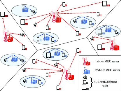
Figure 1: The MEC-enabled HetNet composed of the multi-tier MEC servers and the multi-type users with different size of tasks.

The remainder of this paper is organized as follows. Section II describes the MEC-enabled HetNet model and gives the queueing model for calculating the latency. Section III analyzes the communication latency. Section IV defines and analyzes the SECP. Section V presents the effects of association bias and network parameters on SECP. Finally, conclusions are given in Section VI.

II MEC-enabled Heterogeneous Network Model

In this section, we present the network model and the latency model of the MEC-enabled HetNet.

II-A Network Model

We consider a MEC-enabled HetNet, which is composed of $\mathbf{K}$ tiers of MEC servers, located in APs. An example of the network is given in Fig. 1. MEC servers in different tiers have different transmission and computing capabilities. We use $\mathcal{K}=\{1,\cdots,\mathbf{K}\}$ as the index set of $\mathbf{K}$ tiers of MEC servers. The MEC servers are distributed according to a homogeneous PPP $\mathsf{\mathbb{\Phi}}_{\text{m}}$ with spatial density $\lambda_{\text{m}}$. The locations of the $k$-tier MEC servers are also modeled as a homogeneous PPP $\mathsf{\mathbb{\Phi}}_{\text{m},k}$ with spatial density $\lambda_{\text{m},k}=p_{\text{m},k}\lambda_{\text{m}}$ where $p_{\text{m},k}$ is the portion of the $k$-tier MEC servers. Each servers are assumed to have one CPU and one queue, which has an infinite waiting space. MEC server in a $k$-tier transmits with the power $P_{\text{m},k}$. A channel is assigned to one user only in the cell of MEC server (AP), and the ratio of users using the same uplink channel is $\kappa$, which denotes the frequency reuse factor. The density of uplink interfering users offloading to a $k$-tier MEC server is then given by $\kappa\lambda_{\text{m},k}$.

Computing the large computation task at a mobile device may not be finished within a required time. Hence, users offload their tasks to the MEC servers, which compute/process the tasks and send the resulting data back to the user. Users are categorized into $\mathbf{I}$ types according to the size of their offloading tasks. The $\mathcal{I}=\{1,2,\cdots,\mathbf{I}\}$ denotes the index set of $\mathbf{I}$ type users. A $i$-type user offloads the computation task with $D_{\text{u}i}$ packets to a MEC server. The packet in computation tasks consists of $U_{\text{s}}$ bits. We assume that the both the request message and the resulting data are proportional to the computation task size for simplicity. For that, the user transmits the computation request message in $D_{\text{u}i}$ packets to the MEC server with the power $P_{\text{u},i}$ (i.e., uplink transmission), and receives the computation resulting data in $D_{\text{u}i}$ packets (i.e., downlink transmission).

Each transmission is happened in a time slot $T_{\text{s}}$. The locations of users are modeled as a homogeneous PPP $\mathsf{\mathbb{\Phi}}_{\text{u}}$ with spatial density $\lambda_{\text{u}}$. The $i$-type users are distributed according to a homogeneous PPP $\mathsf{\mathbb{\Phi}}_{\text{u},i}$ with spatial density $\lambda_{\text{u},i}=p_{\text{u},i}\lambda_{\text{u}}$, where $p_{\text{u},i}$ is the portion of the $i$-type users.

Besides the uplink and downlink transmission time, the computation latency at the MEC server is caused when the computation tasks are offloaded to a MEC server. Hence, when an $i$-type user offloads to a $k$-tier MEC server, the total latency of an $i$-type user can be defined as

$$T_{\text{total},i}=T_{\text{cm},i,k}^{(\text{u})}+T_{\text{cm},i,k}^{(\text{d})}+T_{\text{c},i,k}$$ (1)

for $k\geq 1$ where $T_{\text{c},i,k}$ is the computation latency of an $i$-type user at a $k$-tier MEC server. In (1), $T_{\text{cm},i,k}^{(\text{u})}$ and $T_{\text{cm},i,k}^{(\text{d})}$ are the expected uplink transmission time and downlink transmission time, respectively. In this paper, when an $i$-type user offload to a $k$-tier MEC server, $T_{\text{c},i,k}$ is given by $T_{\text{c},i,k}=T_{\text{w},k}+T_{\text{sv},i,k}$, where $T_{\text{w},k}$ is the waiting time at the queue and $T_{\text{sv},i,k}$ is the processing (service) time. To analyze the total latency, both communication latency (i.e., transmission time) and computation latency need to be considered.

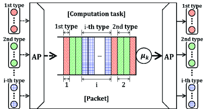
Figure 2: A $k$-tier MEC server when the users offload their computation tasks and receive their resulting data.

TABLE I: Notations used throughout the paper.

Notation	Definition
$\beta_{i,k}^{\left(q\right)}$	Rate coverage probability threshold that an $i$-type user offloads to a $k$-tier MEC server for u, d (u=uplink, d=downlink)
$B_{\text{u}i\triangleright\text{s}k}$	Bias factor of an $i$-type user offloading to a $k$-tier MEC server
$D_{\text{u}i}$	Computation task size of an $i$-type user
$\epsilon_{i,k}^{(q)}$	Target data rate of an $i$-type user offloading to the $k$-tier MEC server for $q=\{\text{u, d}\}$ (u=uplink, d=downlink)
$\lambda_{\text{m},k}$	Spatial density of a $k$-tier MEC server
$\lambda_{\text{u},i}$	Spatial density of an $i$-type user
$\mu_{k}$	Service rate of a $k$-tier MEC server
$\nu_{i,k}$	Arrival rate of an $i$-type user offloading to a $k$-tier MEC server
$P_{\text{u},i}$	Transmission power of an $i$-type user
$P_{\text{m},k}$	Transmission power of an $k$-tier MEC server
$p_{\text{u},i}$	Portion of an $i$-type users
$p_{\text{m},k}$	Portion of a $k$-tier MEC servers
$p_{\text{o},i,k}$	Probability that an $i$-type user offloads to a $k$-tier MEC server
$p_{\text{s},i,k}$	Successful edge computing probability that an $i$-type user offloads to a $k$-tier MEC server
$\mathsf{\mathbb{\Phi}}_{\text{m},k}$	PPP for a $k$-tier MEC server distribution
$\mathsf{\mathbb{\Phi}}_{\text{u},i}$	PPP for an $i$-type user distribution
$T_{\text{cm},i,k}^{(q)}$	Communication latency of an $i$-type user offloading to a $k$-tier MEC server for $q=\{\text{u, d}\}$ (u=uplink, d=downlink)
$T_{\text{sv},i,k}$	Service time of an $i$-type user offloading to a $k$-tier MEC server
$T_{\text{t},i}$	Target latency of an $i$-type user
$T_{\text{w},k}$	Waiting time at a $k$-tier MEC server
$\mathcal{W}_{\text{u}i\triangleright\text{s}k}$	Weighting factor of a $i$-type user offloading to a $k$-tier MEC server
$W^{(q)}$	Bandwidth for $q=\{\text{u, d}\}$ (u=uplink, d=downlink) transmission

II-B Communication Latency Model

In a MEC-enabled HetNet, offloading users have communication latency, when the computation request message are transmitted through uplink channel and its resulting data are received through downlink channel. When an $i$-type user offloads to a $k$-tier MEC server, the rate coverage probability is defined as the probability that the acheivable data rate $R_{i,k}^{\left(q\right)}$ is greater than and equal to the target data rate $\epsilon_{i,k}^{(q)}$ given by

$$p_{\text{cm},i,k}^{\left(q\right)}={\mathbb{P}}\left\{{R_{i,k}^{\left(q\right)}\geq\epsilon_{i,k}^{(q)}}\right\}$$ (2)

for $q=\{\text{u},\text{d}\}$ where u and d indicate the uplink and downlink channels, respectively. If the data rate of the user is less than the target data rate, the data transmission becomes failed. We define the maximum target data rate $\overline{\epsilon}_{i,k}^{(q)}$ guaranteeing a certain level of coverage probability as (3)

$$p_{\text{cm},i,k}^{\left(q\right)}={\mathbb{P}}\left\{{R_{i,k}^{\left(q\right)}\geq\overline{\epsilon}_{i,k}^{(q)}}\right\}\geq\beta_{i,k}^{\left(q\right)}$$ (3)

where $\beta_{i,k}^{\left(q\right)}$ is the target coverage probability. Here the retransmission from communication failure is not considered, which can also be ignored by setting high $\beta_{i,k}^{\left(q\right)}$ (i.e., ignorable communication failures) From (3), we then define the communication latency of $i$-type user for offloading to the $k$-tier MEC server, denoted by $T_{\text{cm},i,k}^{(q)}$, as

$$T_{\text{cm},i,k}^{(q)}=\frac{D_{\text{u}i}U_{\text{s}}}{\overline{\epsilon}_{i,k}^{(q)}}.$$ (4)

II-C Computation Latency Model

Besides the communication latency, offloading users in MEC-enabled HetNet also have the computation latency caused when the computation tasks are computed, i.e., processed in the MEC server in AP. To analyze the computation latency, the arrival rate of the computation tasks and the service time distribution at the MEC server need to be determined.

Since the users are distributed as a PPP, the arrivals of computing tasks at the server follow a Poisson process with a certain arrival rate. Here, the arrival rate for an $i$-type user task to a $k$-tier MEC server, denoted by $\nu_{i,k}$, is determined as

$${\nu_{i,k}=\frac{\beta_{i,k}^{\left(u\right)}\lambda_{\text{u}}p_{\text{u},i}p_{\text{o},i,k}}{\lambda_{\text{m}}p_{\text{m},k}}}$$ (5)

where $p_{\text{o},i,k}$ is the probability that an $i$-type user offloads to a $k$-tier MEC server. When a user offload the computation tasks, we assume a user select a MEC server using the association rule, which is based on the biased average receive power, defined as [19]

$$k=\arg\max_{j\in\mathcal{K}}\left\{\max_{\mathbb{X}_{j}\in\mathsf{\mathbb{\Phi}}_{\text{m},j}}\mathcal{W}_{\text{u}i\triangleright\text{s}j}Z_{\mathbb{x}_{\text{o}},\mathbb{X}_{j}}^{-\alpha}\right\}$$ (6)

where $Z_{\mathbb{x},\mathbb{y}}$ is the distance between $\mathbb{x}$ and $\mathbb{y}$, $\alpha$ is the pathloss exponent, $\mathcal{W}_{\text{u}i\triangleright\text{s}j}=P_{\text{m},j}B_{\text{u}i\triangleright\text{s}j}$ is the weighting factor for an $i$-type user offloading to a $j$-tier MEC server, and $B_{\text{u}i\triangleright\text{s}j}$ is the bias factor. This shows that the $i$-type user located at $\mathbb{x}_{\text{o}}$ is associated to the $k$-tier MEC server. Based on the association rule in (6), $p_{\text{o},i,k}$ in (5) is given by [19]

$$p_{\text{o},i,k}=2\pi\lambda_{\text{m},k}\int_{0}^{\infty}x\exp\left\{-\pi x^{2}\sum_{j\in\mathcal{K}}\lambda_{\text{m},j}\hat{\mathcal{W}}_{\text{u}i\triangleright\text{s}j}^{2/\alpha}\right\}dx$$ (7)

where $\hat{\mathcal{W}}_{\text{u}i\triangleright\text{s}j}$ is $\mathcal{W}_{\text{u}i\triangleright\text{s}j}/\mathcal{W}_{\text{u}i\triangleright\text{s}k}$.

The service rate (i.e., computing capability) of a $k$-tier MEC server $\mu_{k}$ is determined as $\mu_{k}=F_{\text{m},k}/\left(C_{\text{u}}U_{\text{s}}\right)$ where $C_{\text{u}}$ is the number of CPU cycles required for computing $1$ bit of a computation task and $F_{\text{m},k}$ is the computing capacity of $k$-tier MEC server measured by the number of CPU cycles per second. The distribution of the service time for one packet in a $k$-tier MEC server is modeled as the exponential distribution with $1/\mu_{k}$. Since an $i$-type user offloads $D_{\text{u}i}$ packets of the task, $T_{\text{sv},i,k}$ follows the Erlang distribution, and the probability density function (pdf) of $T_{\text{sv},i,k}$, $f_{T_{\text{sv},i,k}}\left(t\right)$, is given by

$$f_{T_{\text{sv},i,k}}\left(t\right)=\frac{\mu_{k}^{D_{\text{u}i}}t^{D_{\text{u}i}-1}\exp\left(-\mu_{k}t\right)}{\left(D_{\text{u}i}-1\right)!}.$$ (8)

The service time in a $k$-tier MEC server, denoted by $T_{\text{sv},k}$, is the weighted sum of $T_{\text{sv},i,k}$ given by $T_{\text{sv},k}=\sum_{i\in\mathcal{I}}\left(\nu_{i,k}/\nu_{k}\right)T_{\text{sv},i,k}$ where $\nu_{k}=\sum_{i\in\mathcal{I}}\nu_{i,k}$ is the arrival rate of users offloading to a $k$-tier MEC server. Hence, the pdf of $T_{\text{sv},k}$ is given by

$$f_{T_{\text{sv},k}}\left(t\right)=\sum_{i\in\mathcal{I}}\left(\frac{\nu_{i,k}}{\nu_{k}}\right)f_{T_{\text{sv},i,k}}\left(t\right).$$ (9)

II-D Performance Metric

For MEC-enabled HetNets, we derive the SECP as the performance metric. The SECP is the probability that the computation in MEC server and communication between MEC server and mobile users are finished within a target latency. According to (1), the SECP for an $i$-type user offloading to a $k$-tier MEC server, denoted by $p_{\text{s},i,k}$, is defined as

$$p_{\text{s},i,k}={\mathbb{P}}\left\{{T_{\text{w},k}+T_{\text{sv},i,k}+T_{\text{cm},i,k}^{(\text{u})}+T_{\text{cm},i,k}^{(\text{d})}\leqq T_{\text{t},i}}\right\}$$ (10)

where $T_{\text{t},i}$ is the target latency of a $i$-type user. The SECP can be considered equivalently to 1) the probability that a user can finish the edge computation within the target latency, and 2) the average fraction of mobile users that satisfy the latency requirements, i.e., latency QoS. Using the law of total probability, the overall SECP for the network is given by

$$p_{\text{s}}=\sum_{k\in\mathcal{K}}\sum_{i\in\mathcal{I}}p_{\text{u},i}p_{\text{o},i,k}p_{\text{s},i,k}.$$ (11)

III Communication Latency Analysis

In this section, we analyze the communication latency i.e., uplink and downlink transmission time, when an $i$-type user communicates with a $k$-tier MEC server. We assume that the channel state information for both users and MEC servers are known, so that both users and MEC servers can determine the data rate satisfying the target coverage probability before transmiting the computation tasks or results. According to (4), the maximum target data rate needs to be determined first to obtain the both uplink and downlink transmission time. The maximum target data rate $\overline{\epsilon}_{i,k}^{(q)}$ is given by

$$\overline{\epsilon}_{i,k}^{(q)}=\int_{y>0}\overline{\epsilon}_{i,k}^{(q)}\left(y\right)f_{Y_{i,k}}\left(y\right)dy$$ (12)

for $q=\{\text{u, d}\}$ where $f_{Y_{i,k}}\left(y\right)$ is the pdf of the distance between the $i$-type user and the associated $k$-tier MEC server denoted by $Y_{i,k}$, given by [19, Lemma 4]

$$f_{Y_{i,k}}\left(y\right)=\frac{2\pi\lambda_{\text{m},k}}{p_{\text{o},i,k}}y\exp\left\{-\pi\sum_{j\in\mathcal{K}}\lambda_{\text{m},j}\hat{\mathcal{W}}_{\text{u}i\triangleright\text{s}j}^{2/\alpha}y^{2}\right\}.$$ (13)

In (12), $\overline{\epsilon}_{i,k}^{(q)}\left(y\right)$ is the maximum target data rate when an $i$-type user offloads to and receives from a $k$-tier MEC server located at $y$. The $\overline{\epsilon}_{i,k}^{(q)}\left(y\right)$ is given by guaranteeing the rate coverage probability $p_{\text{cm},i,k}^{\left(q\right)}$ in (3). The $p_{\text{cm},i,k}^{\left(q\right)}$ can be presented by

$$p_{\text{cm},i,k}^{\left(q\right)}={\mathbb{P}}\left\{{\text{SIR}_{i,k}^{(q)}\left(y\right)\geq 2^{\frac{\overline{\epsilon}_{i,k}^{(q)}}{W^{(u)}}}\!\!-1}\right\}\geq\beta_{i,k}^{\left(q\right)}$$ (14)

for $q=\{\text{u, d}\}$ where $\!W^{(q)}\!$ is the bandwidth, and $\text{SIR}_{i,k}^{(q)}$ is the received signal-to-interference ratio (SIR) when the $i$-type user offloads to and receives from the $k$-tier MEC server located at $y$. For the analytical tractability, some assumptions are used here to derive the uplink transmission time.

1) Assumption 1: The distribution of uplink interfering users follows the PPP.

The uplink interfering user distribution is not a PPP because locations of the users using same uplink channel is from the dependent thinning of the AP locations. However, according to [20], such effect can be weak. Hence, we use this assumption, as in other papers [20, 28], for analysis tractability.

2) Assumption 2: Uplink and downlink interference are independent.

Uplink and downlink interference are not independent because the locations of MEC servers and interfering users are dependent. Although some papers like [29] considered this dependence by a simplified method, it is still complicate to analyze the dependence. As the uplink analysis is not main objective of this work, we apply this assumption.

Using those assumptions and Theorem 1 in [20], the uplink rate coverage probability (i.e., $q=u$) is given by

$$p_{\text{cm},i,k}^{\left(u\right)}=\mathcal{L}_{I_{i,k}^{(u)}}\left\{y^{\alpha}P_{\text{u},i}^{-1}\left(2^{\frac{\overline{\epsilon}_{i,k}^{(u)}}{W^{(u)}}}-1\right)\right\}$$ (15)

where $I_{i,k}^{(u)}$ is the interference when an $i$-type user offloads to a $k$-tier MEC server. The $\mathcal{L}_{I_{i,k}^{(u)}}\left(s\right)$ in (15) is presented as [22]

$$\mathcal{L}_{I_{i,k}^{(u)}}\left(s\right)=\exp\left\{\!-2\pi\lambda_{\text{m}}\int_{z_{i,k}}^{\infty}\frac{x}{1+\left(sP_{\text{u},i}\right)^{-1}x^{\alpha}}dx\right\}$$ (16)

where $z_{i,k}$ is the distance to the nearest $k$-tier MEC server unassociated with the $i$-type user. Since the nearest interfering user can be closer than the associated user, $z_{i,k}$ becomes zero. By replacing $s=y^{\alpha}P_{\text{u},i}^{-1}\left(2^{\overline{\epsilon}_{i,k}^{(u)}/W^{(u)}}\!\!-1\right)$ in (16) and $z_{i,k}=0$, (15) is calculated by

$$p_{\text{cm},i,k}^{\left(u\right)}\!\!= \exp\!\left\{\!\!-2\pi\kappa\lambda_{\text{m}}\!\!\int_{0}^{\infty}\!\!\!\!\!\!\frac{x}{1+\left(y^{-\alpha}/\!\left(2^{\overline{\epsilon}_{i,k}^{(u)}/W^{(u)}}\!\!-1\right)\!\right)\!x^{\alpha}}dx\!\right\}$$

$$= \exp{\left\{-\pi\kappa\lambda_{\text{m}}y^{2}Z\left(2^{\overline{\epsilon}_{i,k}^{(u)}/W^{(u)}}\!\!-1,\alpha,0\right)\right\}}$$ (17)

where $Z\left(a,b,c\right)=a^{2/b}\int_{\left(c/a\right)^{2/b}}^{\infty}\frac{1}{1+u^{b/2}}du$. It is hard to calculate $p_{\text{cm},i,k}^{\left(u\right)}$ for the general path loss. However, for the path loss factor $\alpha=4$, $p_{\text{cm},i,k}^{\left(u\right)}$ can be presented in a tractable form. Using (12) and (III), the uplink maximum target data rate is derived in the following lemma.

Lemma 1

For the uplink transmission with $\alpha=4$, the maximum target data rate $\overline{\epsilon}_{i,k}^{(u)}$ is given by

$$\overline{\epsilon}_{i,k}^{(u)}= \frac{\pi\lambda_{\text{m},k}W^{(u)}}{p_{\text{o},i,k}\ln 2}\biggr{[}\frac{2}{\delta_{1}^{(u)}}\left\{\ln\left(\delta_{2}^{(u)}\right)-\text{ci}\left(\delta_{2}^{(u)}\right)\cos\left(\delta_{2}^{(u)}\right)\right.$$

$$\left.-\text{si}\left(\delta_{2}^{(u)}\right)\sin\left(\delta_{2}^{(u)}\right)+\mathbf{C}\right\}\biggr{]}$$ (18)

where $\delta_{1}^{(u)}$ and $\delta_{2}^{(u)}$ are given, respectively, by

$$\delta_{1}^{(u)}=\pi\sum_{j\in\mathcal{K}}\lambda_{\text{m},j}\hat{\mathcal{W}}_{\text{u}i\triangleright\text{s}j}^{1/2},\indent\delta_{2}^{(u)}=\frac{-2\delta_{1}^{(u)}\ln\beta_{i,k}^{\left(u\right)}}{\pi^{2}\kappa\lambda_{\text{m},k}}.$$ (19)

In (1), $\text{ci}\left(\cdot\right)$, $\text{si}\left(\cdot\right)$, and $\mathbf{C}$ are cosine integral function, sine integral function, and euler constant, respectively.

Proof:

For $\alpha=4$, $p_{\text{cm},i,k}^{\left(u\right)}$ in (III) can be presented as

$$p_{\text{cm},i,k}^{\left(u\right)}=\exp{\left\{-\frac{\pi^{2}}{2}\kappa\lambda_{\text{m}}y^{2}\left(2^{\frac{\overline{\epsilon}_{i,k}^{(u)}}{W^{(u)}}}\!\!-1\right)^{1/2}\right\}}.$$ (20)

From (20) and (14), $\overline{\epsilon}_{i,k}^{(u)}\left(y\right)$ is given by

$$\overline{\epsilon}_{i,k}^{(u)}\left(y\right)=W^{(u)}\log_{2}\left\{1+\left(\frac{-2\ln\beta_{i,k}^{\left(u\right)}}{\pi^{2}\kappa\lambda_{\text{m},k}y^{2}}\right)^{2}\right\}.$$ (21)

Substituting (21) and (13) into (12) and replacing $y$ in $t$ according to $t=y^{2}$, $\overline{\epsilon}_{i,k}^{(u)}$ is presented as

$$\overline{\epsilon}_{i,k}^{(u)}= \frac{\pi\lambda_{\text{m},k}W^{(u)}}{p_{\text{o},i,k}\ln 2}\!\!\int_{0}^{\infty}\!\!\left[\ln\left\{\!t^{2}\!+\!\left(\!\frac{-2\ln\beta_{i,k}^{\left(u\right)}}{\pi^{2}\kappa\lambda_{\text{m},k}}\!\right)^{\!\!\!2}\right\}\!\!-\!\ln\left\{t^{2}\right\}\!\right]$$

$$\times\exp\left\{-\pi\sum_{j\in\mathcal{K}}\lambda_{\text{m},j}\hat{\mathcal{W}}_{\text{u}i\triangleright\text{s}j}^{2/\alpha}t\right\}dt.$$ (22)

From the equations in [31, eq. (4.331), eq. (4.338)], (1) becomes (1). ∎

From the analysis in [19] and [22], the downlink rate coverage probability (i.e., $q=d$) is given by

$$p_{\text{cm},i,k}^{\left(d\right)}=\prod_{j\in\mathcal{K}}\mathcal{L}_{I_{i,j}^{(d)}}\left\{y^{\alpha}P_{\text{m},k}^{-1}\left(2^{\frac{\overline{\epsilon}_{i,k}^{(d)}}{W^{(d)}}}-1\right)\right\}$$ (23)

where $I_{i,j}^{(d)}$ is the interference when an $i$-type user receives from a $j$-tier MEC server. In (23), $\mathcal{L}_{I_{i,j}^{(d)}}\left(s\right)$ is given by substituting $P_{\text{u},i}$ and $z_{i,k}$ in (16) into $P_{\text{m},j}$ and $\hat{\mathcal{W}}_{\text{u}i\triangleright\text{s}j}^{1/\alpha}y$, respectively. By replacing $s=y^{\alpha}P_{\text{m},k}^{-1}\left(2^{\overline{\epsilon}_{i,k}^{(d)}/W^{(d)}}\!\!-1\right)$, (23) is represented by

$$p_{\text{cm},i,k}^{\left(d\right)}$$

$$=\exp\!\left\{\!\!-\!\!\sum_{j\in\mathcal{K}}\!2\pi\lambda_{\text{m},j}\!\!\!\!\right.\left.\int_{\!z_{i,j}}^{\infty}\!\!\!\frac{x}{1\!+\!\!\left(\!\hat{P}_{\text{m},j}^{-1}y^{-\alpha}\!/\!\!\left(2^{\overline{\epsilon}_{i,k}^{(d)}/W^{(d)}}\!\!\!-\!1\!\right)\!\right)\!\!x^{\alpha}}dx\!\!\right\}$$

$$=\exp{\!\left\{\!-\!\!\sum_{j\in\mathcal{K}}\!\pi\hat{P}_{\text{m},j}^{2/\alpha}\!\lambda_{\text{m},j}y^{2}Z\!\left(2^{\overline{\epsilon}_{i,k}^{(d)}/W^{(d)}}\!\!\!\!-\!1,\alpha,\!\hat{B}_{\text{u}i\triangleright\text{s}j}\right)\!\!\right\}}$$ (24)

where $\hat{P}_{\text{m},j}$ is $P_{\text{m},j}/P_{\text{m},k}$ and $\hat{B}_{\text{u}i\triangleright\text{s}j}$ is $B_{\text{u}i\triangleright\text{s}j}/B_{\text{u}i\triangleright\text{s}k}$. Similar with the uplink case, $p_{\text{cm},i,k}^{\left(d\right)}$ can be obtained in a tractable form for the path loss factor $\alpha=4$. However, since $\overline{\epsilon}_{i,k}^{(d)}\left(y\right)$ is included in the $Z$ function in (III), it is difficult to present $\overline{\epsilon}_{i,k}^{(d)}$. For the analytical tractability, we obtain the lower bound of $\overline{\epsilon}_{i,k}^{(d)}$ by approximating $\hat{B}_{\text{u}i\triangleright\text{s}j}$ as $0$. Using (12) and (III), the lower bound of downlink maximum target data rate is derived in the following lemma.

Lemma 2

For the downlink transmission with $\alpha=4$, the lower bound of the maximum target data rate $\hat{\overline{\epsilon}}_{i,k}^{(d)}$ is given by

$$\hat{\overline{\epsilon}}_{i,k}^{(d)}= \frac{\pi\lambda_{\text{m},k}W^{(d)}}{p_{\text{o},i,k}\ln 2}\biggr{[}\frac{2}{\delta_{1}^{(d)}}\left\{\ln\left(\delta_{2}^{(d)}\right)-\text{ci}\left(\delta_{2}^{(d)}\right)\cos\left(\delta_{2}^{(d)}\right)\right.$$

$$\left.-\text{si}\left(\delta_{2}^{(d)}\right)\sin\left(\delta_{2}^{(d)}\right)+\mathbf{C}\right\}\biggr{]}$$ (25)

where $\delta_{1}^{(d)}$ and $\delta_{2}^{(d)}$ are given, respectively, by

$$\delta_{1}^{(d)}=\pi\!\sum_{j\in\mathcal{K}}\!\lambda_{\text{m},j}\hat{\mathcal{W}}_{\text{u}i\triangleright\text{s}j}^{1/2},\indent\!\!\!\!\delta_{2}^{(d)}=\!\frac{-2\delta_{1}^{(d)}\ln\beta_{i,k}^{\left(d\right)}}{\pi^{2}\sum_{j\in\mathcal{K}}\lambda_{\text{m},j}\hat{P}_{\text{m},j}^{1/2}}.$$ (26)

In (1), $\text{ci}\left(\cdot\right)$, $\text{si}\left(\cdot\right)$, and $\mathbf{C}$ are cosine integral function, sine integral function, and euler constant, respectively.

Proof:

For $\alpha=4$, $p_{\text{cm},i,k}^{\left(d\right)}$ in (III) can be presented as

$$p_{\text{cm},i,k}^{\left(d\right)}\!\geq\!\exp{\left\{-\sum_{j\in\mathcal{K}}\frac{\pi^{2}}{2}\hat{P}_{\text{m},j}^{1/2}\lambda_{\text{m},j}y^{2}\!\!\left(2^{\frac{\overline{\epsilon}_{i,k}^{(d)}}{W^{(d)}}}\!\!-1\right)^{\!\!1/2}\right\}}.$$ (27)

From (27) and (14), $\hat{\overline{\epsilon}}_{i,k}^{(d)}$ is obtained by

$$\hat{\overline{\epsilon}}_{i,k}^{(d)}\left(y\right)\!=\!W^{(d)}\log_{2}\!\left[1+\!\left(\frac{-2\ln\beta_{i,k}^{\left(d\right)}}{\pi^{2}y^{2}\sum_{j\in\mathcal{K}}\hat{P}_{\text{m},j}^{1/2}\lambda_{\text{m},j}}\right)^{\!2}\right].$$ (28)

Substituting (28) and (13) into (12) and replacing $y$ in $t$ according to $t=y^{2}$, $\hat{\overline{\epsilon}}_{i,k}^{(d)}$ is presented as

$$\hat{\overline{\epsilon}}_{i,k}^{(d)}= \frac{\pi\lambda_{\text{m},k}W^{(d)}}{p_{\text{o},i,k}\ln 2}\!\!\int_{0}^{\infty}\biggr{[}\ln\left\{\!t^{2}\!+\!\left(\!\frac{-2\ln\beta_{i,k}^{\left(d\right)}}{\pi^{2}\sum_{j\in\mathcal{K}}\lambda_{\text{m},j}\hat{P}_{\text{m},j}^{1/2}}\!\right)^{\!\!\!2}\right\}\!\!$$

$$-\!\ln\left\{t^{2}\right\}\!\biggr{]}\exp\left\{-\pi\sum_{j\in\mathcal{K}}\lambda_{\text{m},j}\hat{\mathcal{W}}_{\text{u}i\triangleright\text{s}j}^{2/\alpha}t\right\}dt.$$ (29)

From the equations in [31, eq. (4.331), eq. (4.338)], (2) becomes (2). ∎

By substituting (1) and (2) into (4), we can derive both uplink and downlink transmission time (i.e., communication latency). Here, we use the lower bound of the target data rate for downlink as it can also guarantee the target coverage probability. From (4), we can show that the communication latency can be changed according to the target coverage probability.

IV Successful Edge Computing Probability Analysis

In this section, we analyze the SECP for an $i$-type user offloading to a $k$-tier MEC server, defined in section II. Using (10) and [32], $p_{\text{s},i,k}$ is derived in the following theorem.

Theorem 1

The SECP for an $i$-type user offloading to a $k$-tier MEC server, denoted by $p_{\text{s},i,k}$, is given by

$$p_{\text{s},i,k}= \int_{0}^{\infty}\!\!\!\int_{0}^{{T_{\text{th},i}-r}}\!\!\!\mathcal{L}_{T_{\text{w},k}}^{-1}\left[\frac{\left(1-\rho_{k}\right)s}{s-\nu_{k}+\nu_{k}\mathcal{L}_{T_{\text{sv},k}}\left(s\right)}\right]$$

$$\times\frac{\mu_{k}^{D_{\text{u}i}}r^{D_{\text{u}i}-1}\exp\left(-\mu_{k}r\right)}{\left(D_{\text{u}i}-1\right)!}dtdr$$ (30)

for $T_{\text{th},i}-r>0$, where $\mathcal{L}_{T_{\text{w},k}}^{-1}\left(s\right)$ is the inverse Laplace transform for pdf of waiting time, $T_{\text{th},i}$ is $T_{\text{t},i}-\sum_{q\in\mathcal{Q}}T_{\text{cm},i,k}^{(q)}$ for $q=\{\text{u, d}\}$, and $\rho_{k}$ is the utilization factor of a $k$-tier MEC server given by

$$\rho_{k}=\sum_{i\in\mathcal{I}}\nu_{i,k}\frac{D_{\text{u}i}}{\mu_{k}}$$ (31)

for $0\leqq\rho_{k}<1$. In (1), $\mathcal{L}_{T_{\text{sv},k}}\left(s\right)$ is the Laplace transform of the pdf of service time in a $k$-tier MEC server given by

$$\mathcal{L}_{T_{\text{sv},k}}\left(s\right)=\sum_{i\in\mathcal{I}}\frac{\nu_{i,k}}{\nu_{k}}\left(\frac{\mu_{k}}{s+\mu_{k}}\right)^{D_{\text{u}i}}.$$ (32)

Proof:

The Laplace transform of the pdf of waiting time is refered to as the Pollaczek-Khinchin (P-K) transform equation of M/G/1 queue in [32]. Using the equation, $\mathcal{L}_{T_{\text{w},k}}(s)$ is given by

$$\mathcal{L}_{T_{\text{w},k}}\left(s\right)=\frac{\left(1-\rho_{k}\right)s}{s-\nu_{k}+\nu_{k}\mathcal{L}_{T_{\text{sv},k}}\left(s\right)}.$$ (33)

The $\mathcal{L}_{T_{\text{w},k}}^{-1}\left(s\right)$ is obtained using (33), which shows the pdf of the waiting time. Since $T_{\text{sv},i,k}$ is a random variable with the pdf in (8), $p_{\text{s},i,k}$ is given by

$$p_{\text{s},i,k}= \int_{0}^{T_{\text{th},i}}\!\!\!\int_{0}^{T_{\text{th},i}-r}\!\!\!\mathcal{L}_{T_{\text{w},k}}^{-1}\left[\frac{\left(1-\rho_{k}\right)s}{s-\nu_{k}+\nu_{k}\mathcal{L}_{T_{\text{sv},k}}\left(s\right)}\right]$$

$$\times f_{T_{\text{sv},i,k}}\left(r\right)dtdr.$$ (34)

According to [32], $\rho_{k}$ and $\mathcal{L}_{T_{\text{sv},k}}\left(s\right)$ are given by, respectively

$$\rho_{k} =\nu_{k}{\mathbb{E}}\left\{{T_{\text{sv},k}}\right\}=\nu_{k}\sum_{i\in\mathcal{I}}\frac{\nu_{i,k}}{\nu_{k}}\frac{D_{\text{u}i}}{\mu_{k}}=\sum_{i\in\mathcal{I}}\nu_{i,k}\frac{D_{\text{u}i}}{\mu_{k}}$$ (35)

$$\mathcal{L}_{T_{\text{sv},k}}\left(s\right) =\sum_{i\in\mathcal{I}}\frac{\nu_{i,k}}{\nu_{k}}\mathcal{L}\left[\frac{\mu_{k}^{D_{\text{u}i}}t^{D_{\text{u}i}-1}\exp\left(-\mu_{k}t\right)}{\left(D_{\text{u}i}-1\right)!}\right]$$

$$=\sum_{i\in\mathcal{I}}\frac{\nu_{i,k}}{\nu_{k}}\left(\frac{\mu_{k}}{s+\mu_{k}}\right)^{D_{\text{u}i}}.$$ (36)

Substituting (35), (IV) and (8) into (33), (IV) becomes (1). ∎

The $p_{\text{s},i,k}$ is hard to be presented in a closed form because of the inverse Laplace transform. However, $p_{\text{s},i,k}$ can be given in a closed form for some cases as the following corollaries.

$$\hat{p}_{\text{s},i,k}= \left(1-\rho_{k}\right)\!\frac{\gamma\left(D_{\text{u}i},\mu_{k}T_{\text{th},i}\right)}{\left(D_{\text{u}i}-1\right)!}\!+\!\rho_{k}\biggr{[}\frac{\gamma\left(\beta_{k,1},\beta_{k,2}T_{\text{th},i}\right)}{\Gamma\left(\beta_{k,1}\right)}\!-\!\frac{\beta_{k,2}^{\beta_{k,1}}\exp\{-\beta_{k,2}T_{\text{th},i}\}}{\Gamma\left(\beta_{k,1}\right)}$$

$$\times\!\sum_{n=0}^{D_{\text{u}i}-1}\!\!\frac{\mu_{k}^{n}}{n!}B\left(\beta_{k,1},n+1\right)T_{\text{th},i}^{\beta_{k,1}+n}{}_{1}F_{1}\!\left(n+1;\beta_{k,1}+n+1;T_{\text{th},i}\left(\beta_{k,2}-\mu_{k}\right)\right)\biggr{]}$$ (46)

 

Corollary 1

For the user type set $\mathcal{I}=\{1\}$ and $D_{\text{u}i}=1$, $p_{\text{s},i,k}$ is given by

$$p_{\text{s},i,k}=1-\exp\left\{\left(-\mu_{k}\!+\!\nu_{k}\right)T_{\text{th},i}\right\}.$$ (37)

Proof:

For the user type set $\mathcal{I}=\{1\}$ and $D_{\text{u}i}=1$, $\mathcal{L}_{T_{\text{sv},k}}\left(s\right)=\frac{\mu_{k}}{s+\mu_{k}}$, so we have

$$\mathcal{L}_{T_{\text{w},k}}\!\!\left(s\right)\!=\!\frac{\left(1-\rho_{k}\right)s}{s-\nu_{k}+\frac{\nu_{k}\mu_{k}}{s+\mu_{k}}}\!=\!\left(1\!-\rho_{k}\right)\!\left\{1\!+\!\frac{\nu_{k}}{s\!+\!\mu_{k}\!-\!\nu_{k}}\!\right\}\!.$$ (38)

Since $\mathcal{L}^{-1}\{\frac{1}{s+\mu_{k}-\nu_{k}}\}=\exp\{\left(-\mu_{k}+\nu_{k}\right)t\}$, $f_{T_{\text{w},k}}\!\left(t\right)\!$, i.e., $\mathcal{L}_{T_{\text{w},k}}^{-1}\left(s\right)$, is presented by

$$f_{T_{\text{w},k}}\!\left(t\right)\!=\!\left(1-\rho_{k}\right)\!\delta\left(t\right)\!+\!\nu_{k}\!\left(1-\rho_{k}\right)\exp\!\left\{\left(-\mu_{k}\!+\!\nu_{k}\right)\!t\right\}$$ (39)

where $\delta\left(t\right)$ is the delta function which means that a user has zero wait with probability $\left(1-\rho_{k}\right)$. Since $T_{\text{sv},i,k}$ in threshold is a random variable, by substituting $\mathcal{L}_{T_{\text{w},k}}^{-1}\left[\!\frac{\left(1-\rho_{k}\right)s}{s-\nu_{k}+\nu_{k}\mathcal{L}_{T_{\text{sv},k}}\left(s\right)}\!\right]$ in (1) into (39) and applying the pdf of $T_{\text{sv},i,k}$, $p_{\text{s},i,k}$ is given by

$$p_{\text{s},i,k}= \frac{\gamma\left(D_{\text{u}i},\mu_{k}T_{\text{th},i}\right)}{\left(D_{\text{u}i}-1\right)!}-\rho_{k}^{1-D_{\text{u}i}}\exp\left\{-\left(\mu_{k}-\nu_{k}\right)T_{\text{th},i}\right\}$$

$$\times\frac{\gamma\left(D_{\text{u}i},\nu_{k}T_{\text{th},i}\right)}{\left(D_{\text{u}i}-1\right)!}$$ (40)

Substituting $D_{\text{u}i}$ into $1$, (1) becomes (37). ∎

Corollary 2

For the user type set $\mathcal{I}=\{1,2\}$ and $D_{\text{u}i}\in\{1,2\}$, $p_{\text{s},i,k}$ is given by

$$p_{\text{s},i,k}= 1-\rho_{k}+\frac{1-\rho_{k}}{\zeta_{1}-\zeta_{2}}\left[-\frac{\left(\zeta_{1}+\mu_{k}\right)^{2}}{\zeta_{1}}\!+\frac{\left(\zeta_{2}+\mu_{k}\right)^{2}}{\zeta_{2}}\!\right.$$

$$\!+\frac{\left(\zeta_{1}+\mu_{k}\right)^{2}}{\zeta_{1}}\!\left(\frac{\mu_{k}}{\mu_{k}+\zeta_{1}}\right)^{\!\!D_{\text{u}i}}\!\!\!\!\!\!\!\exp\left\{\zeta_{1}T_{\text{th},i}\right\}\!\!$$

$$\left.\!-\frac{\left(\zeta_{2}+\mu_{k}\right)^{2}}{\zeta_{2}}\!\left(\frac{\mu_{k}}{\mu_{k}+\zeta_{2}}\right)^{\!\!D_{\text{u}i}}\!\!\!\!\!\!\!\exp\left\{\zeta_{2}T_{\text{th},i}\right\}\!\right]$$ (41)

where $\zeta_{1}$ and $\zeta_{2}$ are given, respectively, by

$$\zeta_{1}=-\mu_{k}+\frac{\nu_{k}}{2}+\sqrt{\frac{\nu_{k}^{2}}{4}+\mu_{k}\left(\nu_{k}-\nu_{1,k}\right)},$$

$$\zeta_{2}=-\mu_{k}+\frac{\nu_{k}}{2}-\sqrt{\frac{\nu_{k}^{2}}{4}+\mu_{k}\left(\nu_{k}-\nu_{1,k}\right)}.$$ (42)

Proof:

For the user type set $\mathcal{I}=\{1,2\}$ and $D_{\text{u}i}\in\{1,2\}$, $\mathcal{L}_{T_{\text{sv},k}}\left(s\right)=\frac{\nu_{1,k}}{\nu_{k}}\frac{\mu_{k}}{s+\mu_{k}}+\frac{\nu_{2,k}}{\nu_{k}}\left(\frac{\mu_{k}}{s+\mu_{k}}\right)^{2}$, so $\mathcal{L}_{T_{\text{w},k}}\left(s\right)$ is given by

$$\mathcal{L}_{T_{\text{w},k}}\left(s\right)= \frac{\left(1-\rho_{k}\right)s}{s-\nu_{k}+\nu_{k}\left(\frac{\nu_{1,k}}{\nu_{k}}\frac{\mu_{k}}{s+\mu_{k}}+\frac{\nu_{2,k}}{\nu_{k}}\left(\frac{\mu_{k}}{s+\mu_{k}}\right)^{2}\right)}$$

$$= \frac{1-\rho_{k}}{\zeta_{1}-\zeta_{2}}\!\!\left\{\!\frac{\left(\zeta_{1}\!+\!\mu_{k}\right)^{2}}{s-\zeta_{1}}\!-\!\frac{\left(\zeta_{2}\!+\!\mu_{k}\right)^{2}}{s-\zeta_{2}}\!+\zeta_{1}\!-\zeta_{2}\!\right\}$$ (43)

where $\zeta_{1}$ and $\zeta_{2}$ are (2), and $\nu_{k}=\nu_{1,k}+\nu_{2,k}$. Since $\mathcal{L}^{-1}\{\frac{1}{s-\zeta_{1}}\}=\exp\{\zeta_{1}t\}$, $f_{T_{\text{w},k}}\!\left(t\right)\!$, i.e., $\mathcal{L}_{T_{\text{w},k}}^{-1}\left(s\right)$, is given by

$$f_{T_{\text{w},k}}\left(t\right)= \left(1-\rho_{k}\right)\delta\left(t\right)+\frac{1-\rho_{k}}{\zeta_{1}-\zeta_{2}}\left[\left(\zeta_{1}+\mu_{k}\right)^{2}\exp\left\{\zeta_{1}t\right\}\right.$$

$$\left.-\left(\zeta_{2}+\mu_{k}\right)^{2}\exp\left\{\zeta_{2}t\right\}\right].$$ (44)

Substituting $\mathcal{L}_{T_{\text{w},k}}^{-1}\left[\!\frac{\left(1-\rho_{k}\right)s}{s-\nu_{k}+\nu_{k}\mathcal{L}_{T_{\text{sv},k}}\left(s\right)}\!\right]$ in (1) into (2), $p_{\text{s},i,k}$ is given by

$$p_{\text{s},i,k}= \int_{0}^{\infty}\!\biggr{[}\frac{1-\rho_{k}}{\zeta_{1}-\zeta_{2}}\biggr{\{}\frac{\left(\zeta_{1}\!+\!\mu_{k}\right)^{2}}{\zeta_{1}}\left(\exp\{\zeta_{1}\left(T_{\text{th},i}-r\right)\}\!-\!1\right)$$

$$\!\!-\!\frac{\left(\zeta_{2}\!+\!\mu_{k}\right)^{2}}{\zeta_{2}}\!\left(\exp\{\zeta_{2}\left(T_{\text{th},i}-r\right)\}\!-\!1\right)\!\biggr{\}}\!+\!\left(1-\rho_{k}\right)\biggr{]}$$

$$\times\frac{\mu_{k}^{D_{\text{u}i}}r^{D_{\text{u}i}-1}\!\exp\!\left(-\mu_{k}r\right)}{\left(D_{\text{u}i}-1\right)!}dr$$ (45)

which is the same as (2). ∎

\psfrag{pcomp}[bc][tc][0.7]{$p_{\text{s}}$, $\hat{p}_{\text{s}}$}\psfrag{targetlatency}[tc][bc][0.7]{$T_{\text{t},i}$ [sec]}\psfrag{pcomp-21}[bl][bl][0.59]{$p_{\text{s},i,k}$ for Corollary \ref{coro:cdf21}}\psfrag{pcomp-212-pui-0.5,0.5}[bl][bl][0.59]{$p_{\text{s},i,k}$ for Corollary \ref{coro:cdf212}}\psfrag{pcomp-2123-ga-pui-0.4,0.2,0.4}[bl][bl][0.59]{$\hat{p}_{\text{s},i,k}$ for Lemma \ref{coro:cdf2123}}\psfrag{pcomp-2123-pui-0.4,0.2,0.4-5-00000}[bl][bl][0.59]{$p_{\text{s},i,k}$ for Lemma \ref{coro:cdf2123} (Simulation)}\includegraphics[width=216.81pt]{Fig_CP.eps}

Figure 3: SECP $p_{\text{s}}$ and approximated SECP $\hat{p}_{\text{s}}$ in $2$ tier MEC-enabled HetNet as a function of the target latency $T_{\text{t},i}$ for different number of user type.

For general cases, we can describe $\hat{p}_{\text{s},i,k}$ as a closed form by approximating the waiting time distribution via Gamma distribution [33] to decrease the computational complexity. The approximated SECP, denoted by $\hat{p}_{\text{s},i,k}$, is presented in the following lemma

Lemma 3

For every user type set $\mathcal{I}$ and $D_{\text{u}i}$, the approximated SECP of an $i$-type user offloading to a $k$-tier MEC server, $\hat{p}_{\text{s},i,k}$, is given by (46), where ${}_{1}F_{1}\!\left(\cdot;\cdot;\cdot\right)$ is the confluent hypergeometric function of the first kind, and $B\left(\cdot,\cdot\right)$ is the beta function. In (46), $\beta_{1}$ and $\beta_{2}$ are defined, respectively, as

$$\beta_{k,1}=\frac{{\mathbb{E}}\left\{{T_{\text{w},k}}\right\}^{2}}{{\mathbb{E}}\left\{{T_{\text{w},k}^{2}}\right\}-{\mathbb{E}}\left\{{T_{\text{w},k}}\right\}^{2}},\indent\beta_{k,2}=\frac{\beta_{k,1}}{{\mathbb{E}}\left\{{T_{\text{w},k}}\right\}}$$ (47)

where ${\mathbb{E}}\left\{{T_{\text{w},k}}\right\}$ and ${\mathbb{E}}\left\{{T_{\text{w},k}^{2}}\right\}$ are given, respectively, by

$${\mathbb{E}}\left\{{T_{\text{w},k}}\right\}=\frac{\sum_{i\in\mathcal{I}}\nu_{i,k}D_{\text{u}i}\left(D_{\text{u}i}+1\right)}{2\mu_{k}^{2}\left(1-\sum_{i\in\mathcal{I}}\nu_{i,k}\frac{D_{\text{u}i}}{\mu_{k}}\right)}$$ (48)

$${\mathbb{E}}\left\{{T_{\text{w},k}^{2}}\right\}\!=\!2{\mathbb{E}}\left\{{T_{\text{w},k}}\right\}^{2}\!+\!\frac{\sum_{i\in\mathcal{I}}\nu_{i,k}D_{\text{u}i}\left(D_{\text{u}i}+1\right)\!\left(D_{\text{u}i}+2\right)}{3\mu_{k}^{3}\left(1\!-\!\sum_{i\in\mathcal{I}}\nu_{i,k}\frac{D_{\text{u}i}}{\mu_{k}}\right)}.$$ (49)

Proof:

See Appendix -A. ∎

TABLE II: Parameter values if not otherwise specified

Parameters	Values	Parameters	Values
$\lambda_{\text{m}}$ [nodes/m2]	$4*10^{-5}$	$\lambda_{\text{u}}$ [nodes/m2]	$12*10^{-4}$
$p_{\text{u},1}$	$0.5$	$p_{\text{u},2}$	$0.5$
$p_{\text{m},1}$	$0.25$	$p_{\text{m},2}$	$0.75$
$W^{(u)}$ [Hz]	$5*10^{6}$	$W^{(d)}$ [Hz]	$10*10^{6}$
$P_{\text{u},i}$ [dBm]	$23$	$P_{\text{m},1}$ [dBm]	$43$
$P_{\text{m},2}$ [dBm]	$33$	$N_{0}$ [dBm]	$-104$
$\alpha$	$4$	$\kappa$	$0.75$
$\beta_{i,k}^{\left(u\right)}$	$0.95$	$\beta_{i,k}^{\left(d\right)}$	$0.95$
$\mu_{1}$ [packet/slot]	$9$	$\mu_{2}$ [packet/slot]	$3$
$U_{\text{s}}$ [KB]	$100$	$C_{\text{u}}$ [cycles/bit]	$1400$
$F_{\text{m},1}$ [Hz]	$10*10^{6}$	$F_{\text{m},2}$ [Hz]	$3*10^{6}$
$T_{\text{s}}$ [sec]	$10^{-3}$

Fig. 3 shows the SECPs of the corollaries, and the approximated SECP of the lemma as a function of $T_{\text{t},i}$ for fixed $p_{\text{o},i,k}$ considering the $2$ tier MEC-enabled HetNet. For this figure, $T_{\text{t},i}$ are set to be equal for all types of users, and other parameters in Table II are used. From Fig. 3, we can see the good match between $\hat{p}_{\text{s}}$ for Lemma 3 and $p_{\text{s}}$ obtained by the simulation for Lemma 3. Hence, the results of Lemma 3 can be used to get the numerical results.

Substituting (7), and (1) into (11), $p_{\text{s}}$ can be derived. From (11), we can see that deriving the optimal bias factors in terms of $p_{\text{s}}$ is hard due to the complex structure. However, we show the existence of the optimal bias factor using numerical results in Section V.

V Numerical Results

In this section, we provide numerical results on the SECP for the MEC-enabled HetNet consisted of $2$ tier networks (except for Fig. 9 that considers $3$ tier networks). The $1$-tier MEC servers have higher computing capabilities than the $2$-tier MEC servers, and computing capabilities for the $2$-tier MEC servers are also higher than the $3$-tier MEC servers. We assume that both $\beta_{i,k}^{\left(u\right)}$ and $\beta_{i,k}^{\left(d\right)}$ are set to be equal. Note that our framework can be easily extended to the network with different values of $\beta_{i,k}^{\left(u\right)}$ and $\beta_{i,k}^{\left(d\right)}$ by simply changing the parameters. The values of parameters used for numerical results are given in Table II according to [34, 35, 5, 36, 37]. The other parameters not presented in Table II are mentioned when the corresponding figures are introduced.

V-A SECP - Impact of Network Parameters

\psfrag{pspcomp}[bc][tc][0.8]{$p_{\text{s}}$, $p_{\text{cp}}$}\psfrag{bdb}[tc][bc][0.7]{$B_{\text{u}1\triangleright\text{s}2}$ [dB]}\psfrag{secp-analysis}[bl][bl][0.59]{Analysis $p_{\text{s}}$}\psfrag{scp-analysis}[bl][bl][0.59]{Analysis $p_{\text{cp}}$}\psfrag{secp-simulation}[bl][bl][0.59]{Simulation $p_{\text{s}}$}\psfrag{scp-simulation}[bl][bl][0.59]{Simulation $p_{\text{cp}}$}\includegraphics[width=216.81pt]{fig-secp-scp-sim.eps}

Figure 4: SECP $p_{\text{s}}$ and SCP $p_{\text{cp}}$ of $2$ tier MEC-enabled HetNet with $1$ user type as a function of bias factor of a $1$-type user to a $2$-tier MEC server $B_{\text{u}1\triangleright\text{s}2}$.

In this subsection, we show how the bias factors in MEC server association affect the SECP for different network parameters via numerical results. To evaluate the SECP, we first define the SCP as the probability that the computation in MEC server is finished within a target latency. The SCP for an $i$-type user offloading to a $k$-tier MEC server, denoted by $p_{\text{cp},i,k}$, is defined by $p_{\text{cp},i,k}={\mathbb{P}}\left\{{T_{\text{w},k}+T_{\text{sv},i,k}\leqq T_{\text{t},i}}\right\}$. The overall SCP $p_{\text{cp}}$ is presented by $p_{\text{cp}}=\sum_{k\in\mathcal{K}}\sum_{i\in\mathcal{I}}p_{\text{u},i}p_{\text{o},i,k}p_{\text{cp},i,k}$.

Fig. 4 shows $p_{\text{s}}$ and $p_{\text{cp}}$ with $1$ type of users (i.e., $\mathcal{I}=\{1\}$ with $D_{\text{u}1}=\{1\}$) as a function of the bias factor $B_{\text{u}1\triangleright\text{s}2}$ when $T_{\text{t},i}=1\times 10^{-3}$s and $B_{\text{u}1\triangleright\text{s}1}=10\text{dB}$. Note that increasing $B_{\text{u}1\triangleright\text{s}2}$ (i.e., x-axis in Fig. 4) means more users offload their required computation to a $2$-tier MEC server than to a $1$-tier MEC server. From Fig. 4, we first see that the simulation results of $p_{\text{cp}}$ matches well with our analysis, while that of $p_{\text{s}}$ does not match well due to the assumptions used in the communication latency analysis. However, we can still see that the trends according to the bias factor are the same.

In addition, from Fig. 4, it can be seen that when $B_{\text{u}1\triangleright\text{s}2}$ is small, both $p_{\text{cp}}$ and $p_{\text{s}}$ are small. This is because the $1$-tier MEC servers are heavy-loaded, and the communication link between a user and the MEC server are long due to the lower MEC server density in $1$-tier $\lambda_{\text{m},1}$ than that of $2$-tier server $\lambda_{\text{m},2}$. On the other hands, as $B_{\text{u}1\triangleright\text{s}2}$ increases, both $p_{\text{cp}}$ and $p_{\text{s}}$ increase because the computation tasks are starting to be offloaded to a $2$-tier MEC server, which can be located closer to the users and less loaded. However, after certain points of $B_{\text{u}1\triangleright\text{s}2}$, both $p_{\text{cp}}$ and $p_{\text{s}}$ decrease since a $2$-tier MEC server becomes heavy-loaded, and the communication link becomes longer. Therefore, there exists the optimal bias factor $B^{*}_{\text{u}1\triangleright\text{s}2}$ (marked by filled diamond marker for $p_{\text{s}}$ and filled rectangle marker for $p_{\text{cp}}$) in terms of $p_{\text{cp}}$ and $p_{\text{s}}$, which are different.

In general HetNets, the optimal bias factor is determined to offload more task to the $2$-tier servers which have the advantage of shorter link distance. On the contrary, when we consider the computing capability of MEC servers and the amount of computation tasks, the optimal bias factor for $p_{\text{cp}}$ is located closer to zero to offload to the high-capable MEC servers. Therefore, $B^{*}_{\text{u}i\triangleright\text{s}k}$ for $p_{\text{s}}$ are larger than $B^{*}_{\text{u}i\triangleright\text{s}k}$ for $p_{\text{cp}}$ as shown in Fig. 4. In other words, the MEC-enabled HetNets has different optimal bias factors from conventional ones, which consider the communication performance only or computation performance only. Specifically, the optimal bias factor is located between the optimal bias factors obtained in terms of computing or communication performance only.

\psfrag{secp}[bc][tc][0.8]{$p_{\text{s}}$}\psfrag{scp}[bc][tc][0.8]{$p_{\text{cp}}$}\psfrag{bdb}[tc][bc][0.7]{$B_{\text{u}2\triangleright\text{s}2}$ [dB]}\psfrag{secp-reference}[bl][bl][0.59]{$\mu_{2}=3$}\psfrag{secp-mu-low}[bl][bl][0.59]{$\mu_{2}=3.45$}\psfrag{secp-mu-high}[bl][bl][0.59]{$\mu_{2}=3.9$}\psfrag{scp-reference}[bl][bl][0.59]{$\mu_{2}=3$}\psfrag{scp-mu-low}[bl][bl][0.59]{$\mu_{2}=3.45$}\psfrag{scp-mu-high}[bl][bl][0.59]{$\mu_{2}=3.9$}\includegraphics[width=216.81pt]{fig-secp-scp-mu.eps}

Figure 5: SECP $p_{\text{s}}$ and SCP $p_{\text{cp}}$ of $2$ tier MEC-enabled HetNet with $2$ user type as a function of bias factor of a $2$-type user to a $2$-tier MEC server $B_{\text{u}2\triangleright\text{s}2}$ for different service rates (i.e., computing capabilities) of a $2$-tier server $\mu_{2}$.

\psfrag{secp}[bc][tc][0.8]{$p_{\text{s}}$}\psfrag{scp}[bc][tc][0.8]{$p_{\text{cp}}$}\psfrag{bdb}[tc][bc][0.7]{$B_{\text{u}2\triangleright\text{s}2}$ [dB]}\psfrag{secp-lbdu-low}[bl][bl][0.59]{$\lambda_{\text{u}}=9.6*10^{-5}$}\psfrag{secp-lbdu-high}[bl][bl][0.59]{$\lambda_{\text{u}}=10.8*10^{-5}$}\psfrag{secp-reference--------}[bl][bl][0.59]{$\lambda_{\text{u}}=12*10^{-5}$}\psfrag{scp-lbdu-low}[bl][bl][0.59]{$\lambda_{\text{u}}=9.6*10^{-5}$}\psfrag{scp-lbdu-high}[bl][bl][0.59]{$\lambda_{\text{u}}=10.8*10^{-5}$}\psfrag{scp-reference--------}[bl][bl][0.59]{$\lambda_{\text{u}}=12*10^{-5}$}\includegraphics[width=216.81pt]{fig-secp-scp-lbdu.eps}

Figure 6: SECP $p_{\text{s}}$ and SCP $p_{\text{cp}}$ of $2$ tier MEC-enabled HetNet with $2$ user type as a function of bias factor of a $2$-type user to a $2$-tier MEC server $B_{\text{u}2\triangleright\text{s}2}$ for different user densities $\lambda_{\text{u}}$.

\psfrag{secpscp}[bc][tc][0.8]{$p_{\text{s}}$, $p_{\text{cp}}$}\psfrag{bdb}[tc][bc][0.7]{$B_{\text{u}2\triangleright\text{s}2}$ [dB]}\psfrag{secp-dit-low}[bl][bl][0.59]{$p_{\text{s}}\text{ }(D_{\text{u}2}=2)$}\psfrag{secp-dit-high}[bl][bl][0.59]{$p_{\text{s}}\text{ }(D_{\text{u}2}=6)$}\psfrag{secp-reference}[bl][bl][0.59]{$p_{\text{s}}\text{ }(D_{\text{u}2}=4)$}\psfrag{scp-dit-low}[bl][bl][0.59]{$p_{\text{cp}}\text{ }(D_{\text{u}2}=2)$}\psfrag{scp-dit-high}[bl][bl][0.59]{$p_{\text{cp}}\text{ }(D_{\text{u}2}=6)$}\psfrag{scp-reference}[bl][bl][0.59]{$p_{\text{cp}}\text{ }(D_{\text{u}2}=4)$}\psfrag{pcomp}[bl][bl][0.59]{$p_{\text{s}}=0.59$}\psfrag{designpcomp}[bl][bl][0.59]{$B^{*}_{\text{u}2\triangleright\text{s}2}\text{ for }p_{\text{cp}}$}\psfrag{ps}[bl][bl][0.59]{$p_{\text{s}}=0.63$}\psfrag{designps}[bl][bl][0.59]{$B^{*}_{\text{u}2\triangleright\text{s}2}\text{ for }p_{\text{s}}$}\includegraphics[width=216.81pt]{fig-secp-dit-rev2.eps}

Figure 7: SECP $p_{\text{s}}$ and SCP $p_{\text{cp}}$ of $2$ tier MEC-enabled HetNet with $2$ user type as a function of bias factor of a $2$-type user to a $2$-tier MEC server $B_{\text{u}2\triangleright\text{s}2}$ for different task sizes of a $2$-type user.

Fig. 5 shows $p_{\text{s}}$ and $p_{\text{cp}}$, respectively, with $2$ types of users (i.e., $\mathcal{I}=\{1,2\}$ with $D_{\text{u}i}=\{1,2\}$) as a function of $B_{\text{u}2\triangleright\text{s}2}$ for different computing capabilities of a $2$-tier MEC server $\mu_{2}$. For this figure, we consider $T_{\text{t},i}=2\times 10^{-3}$s, and $B_{\text{u}1\triangleright\text{s}2}=10$dB. We first see that both optimal bias factors $B^{*}_{\text{u}2\triangleright\text{s}2}$ for $p_{\text{s}}$ and $p_{\text{cp}}$ increase as $\mu_{2}$ increases, since the $2$-tier MEC servers can process the more computation tasks. However, even for large $\mu_{2}$, both $p_{\text{s}}$ and $p_{\text{cp}}$ decrease as $B_{\text{u}2\triangleright\text{s}2}$ increase after $B^{*}_{\text{u}2\triangleright\text{s}2}$ due to the heavy-loaded MEC servers. Therefore, offloading more computation tasks to the high-capable MEC servers generally shows better SECP unless those servers are heavy-loaded. Moreover, from Fig. 5, it can be seen that $B^{*}_{\text{u}2\triangleright\text{s}2}$ for $p_{\text{cp}}$ are smaller than $B^{*}_{\text{u}2\triangleright\text{s}2}$ for $p_{\text{s}}$. As shown in Fig. 4, $p_{\text{cp}}$ only considers the computing capabilities, while $p_{\text{s}}$ considers the both short link distance and high computing capabilities.

Figs. 6 and 7 present $p_{\text{s}}$ and $p_{\text{cp}}$ as a function of $B_{\text{u}2\triangleright\text{s}2}$ for different user densities $\lambda_{\text{u}}$ and computation task sizes of a $2$-type user $D_{\text{u}2}$, respectively, under the same environment of Fig. 5. We can see that as $\lambda_{\text{u}}$ and $D_{\text{u}2}$ increase, both $B^{*}_{\text{u}2\triangleright\text{s}2}$ for $p_{\text{s}}$ and $p_{\text{cp}}$ increase. For small $\lambda_{\text{u}}$ and $D_{\text{u}2}$, $B^{*}_{\text{u}2\triangleright\text{s}2}$ for both $p_{\text{s}}$ and $p_{\text{cp}}$ become smaller because offloading to high-capable servers can achieves higher performance. However, as $\lambda_{\text{u}}$ and $D_{\text{u}2}$ increase, offloading to the $1$-tier MEC servers no longer enhances $p_{\text{s}}$ and $p_{\text{cp}}$ due to the heavy-loaded $1$-tier servers. Hence, $B^{*}_{\text{u}2\triangleright\text{s}2}$ become larger to distribute the tasks to $2$-tier MEC servers. In Fig. 7, we can also see that $B^{*}_{\text{u}2\triangleright\text{s}2}$ for $p_{\text{s}}$ increase even more to not only distribute the tasks, but decrease the link distance increased by $D_{\text{u}2}$. Therefore, when the amount of computation tasks of the network is large, it is better to distribute the arrival of tasks to the low-capable MEC servers instead of offloading the most of tasks to the high-capable servers.

In Fig. 7, it can be seen that as $D_{\text{u}i}$ increases, the difference between $p_{\text{s}}$ when $B_{\text{u}2\triangleright\text{s}2}$ is optimized for $p_{\text{s}}$ and $p_{\text{s}}$ when $B_{\text{u}2\triangleright\text{s}2}$ is optimized for $p_{\text{cp}}$ becomes larger. Specifically, when $D_{\text{u}2}=2$, $p_{\text{s}}$ when $B^{*}_{\text{u}2\triangleright\text{s}2}=6.2$dB (i.e., optimized for $p_{\text{s}}$) is obtained as $0.98$, and $p_{\text{s}}$ when $B^{*}_{\text{u}2\triangleright\text{s}2}=5.6$dB (i.e., optimized for $p_{\text{cp}}$) is obtained as $0.97$. While, when $D_{\text{u}2}=6$, $p_{\text{s}}$ when $B^{*}_{\text{u}2\triangleright\text{s}2}=11$dB (i.e., optimized for $p_{\text{s}}$) is given as $0.63$, and $p_{\text{s}}$ when $B^{*}_{\text{u}2\triangleright\text{s}2}=7.7$dB (i.e., optimized for $p_{\text{cp}}$) is given as $0.59$. This implies that when designing the MEC-enabled HetNet, a bias design using SECP can be more efficient than the conventional design using SCP.

\psfrag{bdb11}[tc][bc][0.7]{$B_{\text{u}1\triangleright\text{s}1}$ [dB]}\psfrag{bdb12}[bc][tc][0.7]{$B_{\text{u}1\triangleright\text{s}2}$ [dB]}\psfrag{pscp}[tc][tc][0.7]{$p_{\text{s}}$}\includegraphics[width=216.81pt]{fig-secp-2tier-bdb.eps}

Figure 8: SECP $p_{\text{s}}$ of $2$ tier MEC-enabled HetNet with $1$ user type as a function of bias factor of a $1$-type user to $1$-tier MEC server $B_{\text{u}1\triangleright\text{s}1}$ and bias factor of a $1$-type user to $2$-tier MEC server $B_{\text{u}1\triangleright\text{s}2}$.

\psfrag{bdb12}[tc][bc][0.7]{$B_{\text{u}1\triangleright\text{s}2}$ [dB]}\psfrag{bdb13}[bc][tc][0.7]{$B_{\text{u}1\triangleright\text{s}3}$ [dB]}\psfrag{pscp}[tc][tc][0.7]{$p_{\text{s}}$}\includegraphics[width=216.81pt]{fig-secp-3tier-bdb-rev1.eps}

Figure 9: SECP $p_{\text{s}}$ of $3$ tier MEC-enabled HetNet with $1$ type user as a function of bias factor of a $1$-type user to $3$-tier MEC server $B_{\text{u}1\triangleright\text{s}2}$ and bias factor of a $1$-type user to $3$-tier MEC server $B_{\text{u}1\triangleright\text{s}3}$.

\psfrag{bdb12}[tc][bc][0.7]{$B_{\text{u}1\triangleright\text{s}2}$ [dB]}\psfrag{bdb22}[bc][tc][0.7]{$B_{\text{u}2\triangleright\text{s}2}$ [dB]}\psfrag{pscp}[tc][tc][0.7]{$p_{\text{cp}}$}\includegraphics[width=216.81pt]{fig-scp-2type-2tier-bdb.eps}

Figure 10: SCP $p_{\text{cp}}$ of $2$ tier MEC-enabled HetNet with $2$ type user as a function of bias factor of a $1$-type user to $2$-tier MEC server $B_{\text{u}1\triangleright\text{s}2}$ and bias factor of a $2$-type user to $2$-tier MEC server $B_{\text{u}2\triangleright\text{s}2}$.

\psfrag{bdb12}[tc][bc][0.7]{$B_{\text{u}1\triangleright\text{s}2}$ [dB]}\psfrag{bdb22}[bc][tc][0.7]{$B_{\text{u}2\triangleright\text{s}2}$ [dB]}\psfrag{pscp}[tc][tc][0.7]{$p_{\text{s}}$}\includegraphics[width=216.81pt]{fig-secp-2type-2tier-bdb.eps}

Figure 11: SECP $p_{\text{s}}$ of $2$ tier MEC-enabled HetNet with $2$ type user as a function of bias factor of a $1$-type user to $2$-tier MEC server $B_{\text{u}1\triangleright\text{s}2}$ and bias factor of a $2$-type user to $2$-tier MEC server $B_{\text{u}2\triangleright\text{s}2}$.

\psfrag{bdb12}[tc][bc][0.7]{$B_{\text{u}1\triangleright\text{s}2}$ [dB]}\psfrag{bdb32}[bc][tc][0.7]{$B_{\text{u}3\triangleright\text{s}2}$ [dB]}\psfrag{pscp}[tc][tc][0.7]{$p_{\text{s}}$}\includegraphics[width=216.81pt]{fig-secp-3type-2tier-bdb.eps}

Figure 12: SECP $p_{\text{s}}$ of $2$ tier MEC-enabled HetNet with $3$ type user as a function of bias factor of a $1$-type user to $2$-tier MEC server $B_{\text{u}1\triangleright\text{s}2}$ and bias factor of a $3$-type user to $2$-tier MEC server $B_{\text{u}3\triangleright\text{s}2}$.

Fig. 8 shows the contour of $p_{\text{s}}$ of $2$-tier network having $1$ types of users (i.e., $\mathcal{I}=\{1\}$ with $D_{\text{u}1}=\{1\}$) as a function of $B_{\text{u}1\triangleright\text{s}1}$ and $B_{\text{u}1\triangleright\text{s}2}$ under the same environment of Fig. 4. It can be seen that the optimal bias factors are determined by the linear function of $B_{\text{u}1\triangleright\text{s}1}$ and $B_{\text{u}1\triangleright\text{s}2}$ because, according to (6), the user association is only adjuisted by the ratio between bias factors $B_{\text{u}1\triangleright\text{s}1}/B_{\text{u}1\triangleright\text{s}2}$.

Fig. 9 shows the contour of $p_{\text{s}}$ of $3$-tier network having $1$-type user as a function of $B_{\text{u}1\triangleright\text{s}2}$ and $B_{\text{u}1\triangleright\text{s}3}$. For this figure, $B_{\text{u}1\triangleright\text{s}1}=10$dB, $T_{\text{t},1}=2\times 10^{-3}$s, $P_{\text{m},3}=23\text{dBm}$, $\lambda_{\text{m},3}=4.5\times 10^{-5}$nodes/m², $\mu_{3}=2$packet/slot, $\beta_{1,3}^{\left(q\right)}=0.95$ for $q=\{$u,d$\}$, and other parameters are same as the Fig. 8. From Figs. 8 and 9, we can find that $B^{*}_{\text{u}1\triangleright\text{s}2}$ in Fig. 8 ($B^{*}_{\text{u}1\triangleright\text{s}2}=8.1$dB when $B^{*}_{\text{u}1\triangleright\text{s}1}=10$dB) is smaller than the one in Fig. 9 ($(B^{*}_{\text{u}1\triangleright\text{s}2},B^{*}_{\text{u}1\triangleright\text{s}3})=(6.5,9)\text{dB}$). This implies that the computation tasks in Fig. 9 are distributed to the additional $3$-tier MEC servers, which can achieve the better performance in terms of $p_{\text{s}}$. It can be seen that the maximum SECP in Fig. 9 (i.e., $p_{\text{s}}=0.95$) is bigger than the one in Fig. 8 (i.e., $p_{\text{s}}=0.93$). Therefore, the SECP can be improved by providing the additional tier of MEC servers.

Fig. 10 and Fig. 11 show the contour of $p_{\text{s}}$ and $p_{\text{cp}}$, respectively, having $2$ types of users (i.e., $\mathcal{I}=\{1,2\}$ with $D_{\text{u}i}=\{1,2\}$) as a function of $B_{\text{u}1\triangleright\text{s}2}$ and $B_{\text{u}2\triangleright\text{s}2}$. First, from Fig. 10, we can see that $p_{\text{cp}}$ decreases more by $B_{\text{u}2\triangleright\text{s}2}$ than by $B_{\text{u}1\triangleright\text{s}2}$. This is because the variation of service time for large size tasks (i.e., $D_{\text{u}2}$) is bigger than that for small size tasks (i.e., $D_{\text{u}1}$), so $p_{\text{cp}}$ becomes more sensitive by the arrival of $D_{\text{u}2}$ size tasks.

By comparing Figs. 10 and 11, we can see that the optimal bias factors for $p_{\text{s}}$ and $p_{\text{cp}}$ are different. From Fig. 10, we can see that even when we offload all tasks of $1$-type user or $2$-type user to a $1$-tier MEC server and no task to a $2$-tier MEC server, i.e., $B^{*}_{\text{u}1\triangleright\text{s}2}=0$ or $B^{*}_{\text{u}2\triangleright\text{s}2}=0$, we can achieve the best performance in terms of $p_{\text{cp}}$. However, it becomes different when we consider the SECP as a performance metric. From Fig. 11, we can see that offloading certain amount of tasks to a $1$-tier MEC server and a $2$-tier MEC server, i.e., $B^{*}_{\text{u}1\triangleright\text{s}2}>0$ or $B^{*}_{\text{u}2\triangleright\text{s}2}>0$, can achieve the best performance in terms of $p_{\text{s}}$. This is because in $p_{\text{s}}$, the communication performance is also considered, which can achieve low performance due to the longer link distance when all users associate to certain tier MEC server. Hence, the communication and computation performance needs to be considered together when we determine the bias factors for MEC server association, which can be also seen for the case with $3$ types of users in Fig. 12.

Fig. 12 shows the contour of $p_{\text{s}}$ having $3$ types of users (i.e., $\mathcal{I}=\{1,2,3\}$ with $D_{\text{u}i}=\{1,2,3\}$) as a function of the ratio of the bias factor $B_{\text{u}1\triangleright\text{s}2}$ and $B_{\text{u}3\triangleright\text{s}2}$ when $B_{\text{u}2\triangleright\text{s}2}=10$dB. We can also see that $p_{\text{s}}$ decreases faster by $B_{\text{u}3\triangleright\text{s}2}$ than $B_{\text{u}1\triangleright\text{s}2}$ due to the large task size of a $3$-type users.

V-B SECP - Network Computation Capability

In this subsection, we have also provided additional design insights by introducing the concept of the network computation capability. The network computation capability $\mathcal{NC}_{\mathbf{K}}$ is defined as the total computing capability, available in the network. Hence, it is proportional to the number of MEC servers and the CPU frequency of each MEC servers, given by

$$\mathcal{NC}_{\mathbf{K}}=\sum_{j\in\mathcal{K}}\lambda_{\text{m},j}^{\theta_{j}}\mu_{j}^{\theta_{k}}=\sum_{j\in\mathcal{K}}\left(\frac{1}{\theta_{j}}\lambda_{\text{m},j}\right)\left(\theta_{j}\mu_{j}\right)$$ (50)

where $\lambda_{\text{m},j}$ and $\mu_{j}$ are the spatial density and computing capability (i.e., service rate) of $j$-tier MEC servers, respectively. In this framework, the number of MEC servers and the CPU frequency of MEC servers are proportional to the spatial density of MEC servers, and the computing capability of MEC servers, respectively. Hence, $\mathcal{NC}_{\mathbf{K}}$ can be presented by $\lambda_{\text{m},j}$ and $\mu_{j}$. The $\theta_{j}$ is the ratio factor of the $j$-tier MEC servers. From (50), we can see that $\mathcal{NC}_{\mathbf{K}}$ remains unchanged even when $\theta_{j}$ increases or decreases. For instance, if $\theta_{j}$ increases, the $\mu_{j}$ increases, but $\lambda_{\text{m},j}$ decreases. From Figs. 13 and 14, we discuss how to deploy MEC servers when $\mathcal{NC}_{\mathbf{K}}$ is given. To this end, we have adjusted the density of MEC servers as $\lambda_{\text{m},j}/\theta_{j}$ and the CPU frequency as $\theta_{j}\mu_{j}$ to see their impact when $\mathcal{NC}_{\mathbf{K}}$ is fixed.

\psfrag{secp}[bc][tc][0.8]{$p_{\text{s}}$}\psfrag{ratio}[tc][bc][0.7]{$\theta_{2}$}\psfrag{secp-reference---------}[bl][bl][0.59]{$\mathcal{NC}_{2}=18*10^{-5}$}\psfrag{secp-ncc-low}[bl][bl][0.59]{$\mathcal{NC}_{2}=22.5*10^{-5}$}\psfrag{secp-ncc-high}[bl][bl][0.59]{$\mathcal{NC}_{2}=27*10^{-5}$}\includegraphics[width=216.81pt]{fig-secp-ncc-1tier-rev1.eps}

Figure 13: SECP $p_{\text{s}}$ of $2$ tier MEC-enabled HetNet with $2$ user type as a function of ratio factor $\theta_{2}$ for different network computation capability $\mathcal{NC}_{2}$.

\psfrag{secp}[bc][tc][0.8]{$p_{\text{s}}$}\psfrag{bdb}[tc][bc][0.7]{$B_{\text{u}2\triangleright\text{s}2}$ [dB]}\psfrag{secp-reference----}[bl][bl][0.59]{$\theta_{1}=1$, $\mathbf{K}=1$}\psfrag{secp-ratio-low1}[bl][bl][0.59]{$\theta_{2}=0.8$, $\mathbf{K}=2$}\psfrag{secp-ratio-equal}[bl][bl][0.59]{$\theta_{2}=1$, $\mathbf{K}=2$}\psfrag{secp-ratio-high1}[bl][bl][0.59]{$\theta_{2}=1.2$, $\mathbf{K}=2$}\includegraphics[width=216.81pt]{fig-secp-ncc-2tier-rev1.eps}

Figure 14: SECP $p_{\text{s}}$ of $1$ and $2$ tier MEC-enabled HetNet with $2$ user type as a function of bias factor of a $2$-type user to a $2$-tier MEC server $B_{\text{u}2\triangleright\text{s}2}$ for different ratio factor $\theta_{2}$.

Fig. 13 shows $p_{\text{s}}$ as a function of $\theta_{2}$ for different network computation capabilities $\mathcal{NC}_{\mathbf{K}}$. For this figure, $\theta_{1}=1$, $B_{\text{u}2\triangleright\text{s}2}=15$dB, and other parameters are same as Fig. 5. We can see that as $\theta_{2}$ becomes larger, $p_{\text{s}}$ increases to the optimal points. For small $\theta_{2}$, in spite of the short link distance due to the high MEC server density in $2$-tier $\lambda_{\text{m},2}$, low computing capability of $2$-tier MEC server $\mu_{2}$ cause the degradation of $p_{\text{s}}$. As $\theta_{2}$ increases, $\mu_{2}$ increase, which can achieve higher $p_{\text{s}}$ even though $\lambda_{\text{m},2}$ gradually decreases. However, for excessively high $\theta_{2}$, the larger communication latency due to the low $\lambda_{\text{m},2}$ leads to the decrease in $p_{\text{s}}$ in spite of the high $\mu_{2}$.

Moreover, it can be seen that as $\mathcal{NC}_{\mathbf{K}}$ increases, $p_{\text{s}}$ becomes higher. Consequently, as $\mathcal{NC}_{\mathbf{K}}$ increases, the optimal $\theta_{2}$ maximizing $p_{\text{s}}$ also becomes higher. This implies that when $\mathcal{NC}_{\mathbf{K}}$ is large, the optimal $\theta_{2}$ is determined to increase $\mu_{2}$ rather than $\lambda_{\text{m},2}$. Hence, when the total computation capability deployed in the network is fixed, increasing the computing capability and reducing the number of MEC servers are more beneficial to enhance the SECP.

Fig. 14 presents $p_{\text{s}}$ as a function of $B_{\text{u}2\triangleright\text{s}2}$ for the single tier network and $2$ tier network with different ratio factor $\theta_{2}$. For the single tier network, the total MEC server density $\lambda_{\text{m}}$ is same as $\lambda_{\text{m}}$ for the $2$ tier network, and the computing capability of MEC server $\mu_{1}$ is determined so that $\mathcal{NC}_{1}$ for the single tier network has same value with $\mathcal{NC}_{2}$ for $2$ tier network. Other parameters for single tier network are same as the $1$-tier network in the $2$ tier MEC-enabled HetNet

It can be seen that $p_{\text{s}}$ for multi-tier cases can be larger than $p_{\text{s}}$ for single-tier case. Specifically, for $B_{\text{u}2\triangleright\text{s}2}$ in the range from $1.4$dB to $13.2$dB when $\theta_{2}=1$, $p_{\text{s}}$ for $2$ tier network is larger than $0.77$, which is the value of $p_{\text{s}}$ for single tier network. This implies that extending the single-tier to multi-tier networks can achieve higher $p_{\text{s}}$ without increasing the $\mathcal{NC}_{\mathbf{K}}$ when $B_{\text{u}2\triangleright\text{s}2}$ is adjusted by considering both the computation and the communication performance. Therefore, when the network computation capability is fixed, the SECP in multi-tier networks can be higher than the SECP in single-tier networks by adjusting the association bias factor.

Moreover, we can see that $B^{*}_{\text{u}2\triangleright\text{s}2}$ for $\theta_{2}=1.2$ is larger than the one for $\theta_{2}=0.8$. As $\theta_{2}$ increases, the computing capabilities of $2$-tier MEC servers $\mu_{2}$ become larger and the density of $2$-tier servers $\lambda_{\text{m},2}$ becomes smaller. As a result, the users who offload to the $2$-tier MEC servers can have higher $p_{\text{s}}$ because the total arrivals to $2$-tier server decrease due to the low $\lambda_{\text{m},2}$, and high $\mu_{2}$. Hence, $B^{*}_{\text{u}2\triangleright\text{s}2}$ becomes larger to distribute the tasks to the $2$-tier MEC servers.

VI Conclusions

In this paper, we propose the MEC-enabled HetNet, composed of the multi-type users with different computation task sizes and the multi-tier MEC servers with different computing capacities. We derive the SECP by analyzing the distribution of total latency in MEC-enabled HetNet. With the consideration of both the computing time in MEC server and the transmission time depending on the target coverage probability, the closed form of SECP for special cases, and the approximated SECP for general case are obtained. We then evaluate the effects of bias factors in association and network parameters on the SECP.

Our results provide some insights on the design of MEC-enabled HetNet. Specifically, 1) the MEC-enabled HetNet has different optimal association bias factors from conventional ones, which consider the communication performance only or the computation performance only, and the optimal bias factor is located between the optimal bias factors obtained in terms of computing or communication performance only, 2) offloading more computation tasks to the high-capable MEC servers generally shows better SECP unless those servers are heavy-loaded, 3) when the computation tasks of the network becomes large, it is better to distribute the arrival of tasks to the low-capable MEC servers instead of offloading the most of all tasks to the high-capable MEC servers, 4) when the total computation capability deployed in the network is fixed, increasing the computing capability and reducing the number of MEC servers are more beneficial to enhance the SECP, and 5) when the network computation capability is fixed, the SECP in multi-tier networks can be higher than the SECP in single-tier networks.

-A Proof of Lemma 3

To derive the SECP, the cumulative density function (cdf) of the waiting time at the MEC servers (i.e., M/G/1 queue) is required, which has no closed form to the best of our knowledge. Hence, we approximate the distribution of the waiting time to the Gamma distribution after calculating the Gamma distribution-related parameters such as $\beta_{k,1}$ and $\beta_{k,2}$ in (47), respectively. According to [32], the cdf of the waiting time $F\left(t\right)$, obtained by performing the inverse Laplace transform of (33), is presented by

$$F\left(t\right)=1-\rho_{k}+\rho_{k}F_{\Gamma}\left(t\right)$$ (51)

where $\rho_{k}$ is the utilization factor and $F_{\Gamma}\left(t\right)$ is the cdf of the waiting time for tasks, which are not immediately served upon arrival. We approximate $F_{\Gamma}\left(t\right)$ to the Gamma distribution, which is also applied in [33]. By using the Takacs Recursion Formula in [32], the mean waiting time and the mean square of waiting time for $k$-tier MEC server is obtained by

$${\mathbb{E}}\left\{{T_{\text{w},k}}\right\}=\frac{\sum_{i\in\mathcal{I}}\nu_{i,k}{\mathbb{E}}\left\{{T_{\text{sv},i,k}^{2}}\right\}}{2\left(1-\rho_{k}\right)}$$ (52)

$${\mathbb{E}}\left\{{T_{\text{w},k}^{2}}\right\}=2{\mathbb{E}}\left\{{T_{\text{w},k}}\right\}^{2}+\frac{\sum_{i\in\mathcal{I}}\nu_{i,k}{\mathbb{E}}\left\{{T_{\text{sv},i,k}^{3}}\right\}}{3\left(1-\rho_{k}\right)}$$ (53)

where ${\mathbb{E}}\left\{{\!T_{\text{sv},i,k}^{2}\!}\right\}$ and ${\mathbb{E}}\left\{{\!T_{\text{sv},i,k}^{3}\!}\right\}$ are defined, respectively, by

$${\mathbb{E}}\left\{{\!T_{\text{sv},i,k}^{2}\!}\right\}\!=\!\!\int_{0}^{\infty}\!\!\!\!t^{2}\!f_{T_{\text{sv},i,k}}\!\!\left(t\right)\!dt\!=\!\frac{D_{\text{u}i}\!\left(D_{\text{u}i}+1\right)}{\mu_{k}^{2}}$$ (54)

$${\mathbb{E}}\left\{{\!T_{\text{sv},i,k}^{3}\!}\right\}\!=\!\!\int_{0}^{\infty}\!\!\!\!t^{3}\!f_{T_{\text{sv},i,k}}\!\!\left(t\right)\!dt\!=\!\frac{D_{\text{u}i}\!\left(D_{\text{u}i}+1\right)\!\left(D_{\text{u}i}+2\right)}{\mu_{k}^{3}}.$$ (55)

By matching the (52) and (53) to a mean and variance of Gamma distribution, the Gamma distribution-related parameters $\beta_{k,1}$ and $\beta_{k,2}$ are obtained by (47). Applying the (47), the approximated cdf of the waiting time $\hat{F}\left(t\right)$ is given by

$$\hat{F}\left(t\right)=1-\rho_{k}+\rho_{k}\frac{\gamma\left(\beta_{k,1},\beta_{k,2}t\right)}{\Gamma\left(\beta_{k,1}\right)}$$ (56)

for $t\geq 0$ where $\gamma\left(\cdot,\cdot\right)$ and $\Gamma\left(\cdot,\cdot\right)$ are the lower and upper incomplete gamma function, respectively. Substituting the part of the equation (1) into (56), $\hat{p}_{\text{s},i,k}$ is obtained by

$$\hat{p}_{\text{s},i,k}= \int_{0}^{\infty}\left[1-\rho_{k}+\rho_{k}\hat{F}\left(T_{\text{th},i}-r\right)\right]f_{T_{\text{sv},i,k}}\left(r\right)dr$$

$$= \left(1-\rho_{k}\right)F_{\gamma,1}+\rho_{k}F_{\gamma,2}$$ (57)

where $T_{\text{th},i}$ is $T_{\text{t}}-\sum_{q\in\mathcal{Q}}T_{\text{cm},i,k}^{(q)}$ for $q=\{\text{u},\text{d}\}$. In (-A), $F_{\gamma,1}$ and $F_{\gamma,2}$ are given, respectively, by

$$F_{\gamma,1}\!\!=\!\!\int_{0}^{T_{\text{th},i}}\!\!\frac{\mu_{k}^{D_{\text{u}i}}r^{D_{\text{u}i}\!-1}\!\exp\{\!-\mu_{k}r\!\}}{\left(D_{\text{u}i}-1\right)!}dr\!=\!\frac{\gamma(D_{\text{u}i},\mu_{k}T_{\text{th},i})}{\left(D_{\text{u}i}-1\right)!}$$ (58)

$$F_{\gamma,2}\!=\!\! \int_{0}^{T_{\text{th},i}}\!\!\frac{\gamma\!\left(\beta_{k,1},\beta_{k,2}\!\left(T_{\text{th},i}\!-\!r\right)\right)}{\Gamma\left(\beta_{k,1}\right)}\frac{\mu_{k}^{D_{\text{u}i}}r^{D_{\text{u}i}-1}\exp\{\!-\mu_{k}r\}}{\left(D_{\text{u}i}-1\right)!}dr$$

$$= \frac{\gamma\!\left(\beta_{k,1},\beta_{k,2}T_{\text{th},i}\right)}{\Gamma\left(\beta_{k,1}\right)}-\frac{\!\exp\left\{-\beta_{k,2}T_{\text{th},i}\right\}}{\beta_{k,2}^{-\beta_{k,1}}\Gamma\left(\beta_{k,1}\right)}$$

$$\times\sum_{n=0}^{D_{\text{u}i}-1}\!\frac{\mu_{k}^{n}}{n!}\!\int_{0}^{T_{\text{th},i}}\!\frac{\exp\{\left(\beta_{k,2}\!-\!\mu_{k}\right)r\}r^{k}}{\left(T_{\text{th},i}-r\right)^{1-\beta_{k,1}}}dr.$$ (59)

From the equation in [31, eq. (3.383)], $F_{\gamma,2}$ is provided as the closed-form equations. By substituting the (58) and (-A) into (-A), the approximated SECP becomes (46).

References

• [1] C. Park and J. Lee, “Successful edge computing probability analysis in heterogeneous networks,” in Proc. IEEE Int. Conf. Commun., Kansas City, MO, May 2018, pp. 1–6.
• [2] P. Mach and Z. Becvar, “Mobile edge computing: A survey on architecture and computation offloading,” IEEE Commun. Surveys Tuts., vol. 19, no. 3, pp. 1628–1656, Mar. 2017.
• [3] T. X. Tran, A. Hajisami, P. Pandey, and D. Pompili, “Collaborative mobile edge computing in 5G networks: New paradigms, scenarios, and challenges,” IEEE Commun. Lett., vol. 55, no. 4, pp. 54–61, Apr. 2017.
• [4] Y. Mao, C. You, J. Zhang, K. Huang, and K. B. Letaief, “A survey on mobile edge computing: The communication perspective,” IEEE Commun. Surveys Tuts., vol. 19, no. 4, pp. 2322–2358, Aug. 2017.
• [5] C. You, K. Huang, H. Chae, and B.-H. Kim, “Energy-efficient resource allocation for mobile-edge computation offloading,” IEEE Trans. Wireless Commun., vol. 16, no. 3, pp. 1397–1411, Mar. 2017.
• [6] X. Tao, K. Ota, M. Dong, H. Qi, and K. Li, “Performance guaranteed computation offloading for mobile-edge cloud computing,” IEEE Wireless Commun. Lett., vol. 6, no. 6, pp. 774–777, Dec. 2017.
• [7] T. Q. Dinh, J. Tang, Q. D. La, and T. Q. Quek, “Offloading in mobile edge computing: Task allocation and computational frequency scaling,” IEEE Trans. Commun., vol. 65, no. 8, pp. 3571–3584, Apr. 2017.
• [8] Y. Mao, J. Zhang, S. Song, and K. B. Letaief, “Power-delay tradeoff in multi-user mobile-edge computing systems,” in Proc. IEEE Global Telecomm. Conf., Washington, DC, USA, Dec. 2016, pp. 1–6.
• [9] S. Sardellitti, G. Scutari, and S. Barbarossa, “Joint optimization of radio and computational resources for multicell mobile-edge computing,” IEEE Trans. Signal Inf. Process. Netw., vol. 1, no. 2, pp. 89–103, Jun. 2015.
• [10] F. Wang, J. Xu, X. Wang, and S. Cui, “Joint offloading and computing optimization in wireless powered mobile-edge computing systems,” IEEE Trans. Wireless Commun., vol. 17, no. 3, pp. 1784–1797, Mar. 2018.
• [11] J. Zhang, X. Hu, Z. Ning, E. C.-H. Ngai, L. Zhou, J. Wei, J. Cheng, and B. Hu, “Energy-latency tradeoff for energy-aware offloading in mobile edge computing networks,” IEEE Internet Things J., vol. 5, no. 4, pp. 2633–2645, Aug. 2018.
• [12] J. Liu, Y. Mao, J. Zhang, and K. B. Letaief, “Delay-optimal computation task scheduling for mobile-edge computing systems,” in Proc. IEEE Int. Symp. on Inf. Theory, Barcelona, Spain, Jul. 2016, pp. 1451–1455.
• [13] T. Zhao, S. Zhou, X. Guo, and Z. Niu, “Tasks scheduling and resource allocation in heterogeneous cloud for delay-bounded mobile edge computing,” in Proc. IEEE Int. Conf. Commun., Paris, France, May 2017, pp. 1–7.
• [14] S.-W. Ko, K. Han, and K. Huang, “Wireless networks for mobile edge computing: Spatial modeling and latency analysis,” IEEE Trans. Wireless Commun., vol. 17, no. 8, pp. 5225–5240, Jun. 2018.
• [15] M. Chen and Y. Hao, “Task offloading for mobile edge computing in software defined ultra-dense network,” IEEE J. Sel. Areas Commun., vol. 36, no. 3, pp. 587–597, Mar. 2018.
• [16] J. Zhao, Q. Li, Y. Gong, and K. Zhang, “Computation offloading and resource allocation for cloud assisted mobile edge computing in vehicular networks,” IEEE Trans. Veh. Technol., vol. 68, no. 8, pp. 7944–7956, Aug. 2019.
• [17] Z. Liang, Y. Liu, T.-M. Lok, and K. Huang, “Multiuser computation offloading and downloading for edge computing with virtualization,” IEEE Trans. Wireless Commun., vol. 18, no. 9, pp. 4298–4311, Sep. 2019.
• [18] H. S. Dhillon, R. K. Ganti, F. Baccelli, and J. G. Andrews, “Modeling and analysis of k-tier downlink heterogeneous cellular networks,” IEEE J. Sel. Areas Commun., vol. 30, no. 3, pp. 550–560, Mar. 2012.
• [19] S. Singh, H. S. Dhillon, and J. G. Andrews, “Offloading in heterogeneous networks: Modeling, analysis, and design insights,” IEEE Trans. Wireless Commun., vol. 12, no. 5, pp. 2484–2497, May 2013.
• [20] T. D. Novlan, H. S. Dhillon, and J. G. Andrews, “Analytical modeling of uplink cellular networks,” IEEE Trans. Wireless Commun., vol. 12, no. 6, pp. 2669–2679, Jun. 2013.
• [21] S. Singh, X. Zhang, and J. G. Andrews, “Joint rate and SINR coverage analysis for decoupled uplink-downlink biased cell associations in hetnets,” IEEE Trans. Wireless Commun., vol. 14, no. 10, pp. 5360–5373, Oct. 2015.
• [22] H.-S. Jo, Y. J. Sang, P. Xia, and J. G. Andrews, “Heterogeneous cellular networks with flexible cell association: A comprehensive downlink SINR analysis,” IEEE Trans. Wireless Commun., vol. 11, no. 10, pp. 3484–3495, Oct. 2012.
• [23] Q. Zhang, H. H. Yang, T. Q. Quek, and J. Lee, “Heterogeneous cellular networks with LoS and NLoS transmissions–the role of massive MIMO and small cells,” IEEE Trans. Wireless Commun., vol. 16, no. 12, pp. 7996–8010, Dec. 2017.
• [24] F. Baccelli and B. Błaszczyszyn, Stochastic Geometry and Wireless Networks, Volume I — Theory, ser. Foundations and Trends in Networking.   NoW Publishers, 2009.
• [25] H. Cho, C. Liu, J. Lee, T. Noh, and T. Q. Quek, “Impact of elevated base stations on the ultra-dense networks,” IEEE Commun. Lett., vol. 22, no. 6, pp. 1268–1271, Jun. 2018.
• [26] Y. Zhong, T. Q. Quek, and X. Ge, “Heterogeneous cellular networks with spatio-temporal traffic: Delay analysis and scheduling,” IEEE J. Sel. Areas Commun., vol. 35, no. 6, pp. 1373–1386, Mar. 2017.
• [27] H. H. Yang and T. Q. Quek, “Sir coverage analysis in cellular networks with temporal traffic: a stochastic geometry approach,” arXiv preprint arXiv:1801.09888, Jan. 2018. [Online]. Available: http://arxiv.org/abs/1801.09888
• [28] H. ElSawy and E. Hossain, “On stochastic geometry modeling of cellular uplink transmission with truncated channel inversion power control,” IEEE Trans. Wireless Commun., vol. 13, no. 8, pp. 4454–4469, Aug. 2014.
• [29] J. Lee and T. Q. Quek, “Hybrid full-/half-duplex system analysis in heterogeneous wireless networks,” IEEE Trans. Wireless Commun., vol. 14, no. 5, pp. 2883–2895, May 2015.
• [30] W. U. Mondal and G. Das, “Uplink user process in poisson cellular network,” IEEE Wireless Commun. Lett., vol. 21, no. 9, pp. 2013–2016, Sep. 2017.
• [31] I. S. Gradshteyn and I. M. Ryzhik, Table of Integrals, Series, and Products.   San Diego, CA: Academic Press, Inc., 2007.
• [32] L. Kleinrock, Queueing Systems, Volume 1: Theory.   New York: Wiley-Interscience, 1975.
• [33] M. Menth, R. Henjes, C. Zepfel, and P. Tran-Gia, “Gamma-approximation for the waiting time distribution function of M/G/1 queue,” in Proc. 2nd Conference on Next Generation Internet Design and Engineering, Valencia, Spain, Jan. 2006.
• [34] D. Lopez-Perez, I. Guvenc, G. De la Roche, M. Kountouris, T. Q. Quek, and J. Zhang, “Enhanced inter-cell interference coordination challenges in heterogeneous networks,” IEEE Wireless Commun., vol. 18, no. 3, pp. 22–30, Jun. 2011.
• [35] A. Damnjanovic, J. Montojo, Y. Wei, T. Ji, T. Luo, M. Vajapeyam, T. Yoo, O. Song, and D. Malladi, “A survey on 3gpp heterogeneous networks,” IEEE Wireless Commun., vol. 18, no. 3, pp. 10–21, Jun. 2011.
• [36] X. Chen, L. Jiao, W. Li, and X. Fu, “Efficient multi-user computation offloading for mobile-edge cloud computing,” IEEE/ACM Trans. Netw., vol. 24, no. 5, pp. 2795–2808, Oct. 2015.
• [37] C.-F. Liu, M. Bennis, and H. V. Poor, “Latency and reliability-aware task offloading and resource allocation for mobile edge computing,” in Proc. IEEE Global Telecomm. Conf. Workshops, Singapore, Singapore, Dec. 2017, pp. 1–7.