The XMM-SERVS survey: new XMM-Newton point-source catalog for the XMM-LSS field

\par\LTX@newpageAbstract

We present an X-ray point-source catalog from the XMM-Large Scale Structure survey region (XMM-LSS), one of the XMM-Spitzer Extragalactic Representative Volume Survey (XMM-SERVS) fields. We target the XMM-LSS region with $1.3$ Ms of new XMM-Newton AO-15 observations, transforming the archival X-ray coverage in this region into a 5.3 deg² contiguous field with uniform X-ray coverage totaling $2.7$ Ms of flare-filtered exposure, with a $46$ ks median PN exposure time. We provide an X-ray catalog of 5242 sources detected in the soft (0.5–2 keV), hard (2–10 keV), and/or full (0.5–10 keV) bands with a 1% expected spurious fraction determined from simulations. A total of 2381 new X-ray sources are detected compared to previous source catalogs in the same area. Our survey has flux limits of $1.7\times 10^{-15}$, $1.3\times 10^{-14}$, and $6.5\times 10^{-15}$ erg cm^-2 s^-1 over 90% of its area in the soft, hard, and full bands, respectively, which is comparable to those of the XMM-COSMOS survey. We identify multiwavelength counterpart candidates for 99.9% of the X-ray sources, of which 93% are considered as reliable based on their matching likelihood ratios. The reliabilities of these high-likelihood-ratio counterparts are further confirmed to be $\approx 97\%$ reliable based on deep Chandra coverage over $\approx 5\%$ of the XMM-LSS region. Results of multiwavelength identifications are also included in the source catalog, along with basic optical-to-infrared photometry and spectroscopic redshifts from publicly available surveys. We compute photometric redshifts for X-ray sources in 4.5 deg² of our field where forced-aperture multi-band photometry is available; $>70$% of the X-ray sources in this subfield have either spectroscopic or high-quality photometric redshifts.

1 Introduction

Table 1: Current and scheduled 1–10 deg² multiwavelength coverage of the XMM-SERVS fields. References: [a] Franzen et al. (2015); [b] Jarvis et al. (2017); [c] Oliver et al. (2012); [d] Lonsdale et al. (2003); [e] Mauduit et al. (2012). Note that SERVS has recently been expanded to cover the full LSST deep drilling fields (Spitzer Program ID 11086). [f] Jarvis et al. (2012); [g] http://www.ast.cam.ac.uk/~mbanerji/VEILS/veils_index.html; [h] http://euclid2017.london/slides/Monday/Session3/SurveyStatus-Scaramella.pdf; [i] Diehl et al. (2014); [j] Aihara et al. (2018); [k] Tonry et al. (2012); [l] Vaccari et al. (2016); [m] http://www.lsst.org/News/enews/deep-drilling-201202.html; [n] Kelson et al. (2014); Patel et al. (2015); [o] Coil et al. (2011); [p] https://devilsurvey.org/wp/; [q] http://www.roe.ac.uk/~ciras/MOONS/VLT-MOONS.html; [r] Takada et al. (2014); [s] http://www.galex.caltech.edu/researcher/techdoc-ch2.html. [t] http://personal.psu.edu/wnb3/xmmservs/xmmservs.html.

Band	Survey Name	Coverage (XMM-LSS, W-CDF-S, ELAIS-S1); Notes
Radio	Australia Telescope Large Area Survey (ATLAS)a	–, 3.7, 2.7 deg2; 15 $\mu$Jy rms depth at 1.4 GHz
	MIGHTEE Survey (Starting Soon)b	4.5, 3, 4.5 deg2; 1 $\mu$Jy rms depth at 1.4 GHz
FIR	Herschel Multi-tiered Extragal. Surv. (HerMES)c	0.6–18 deg2; 5–60 mJy depth at 100–500 $\mu$m
MIR	Spitzer Wide-area IR Extragal. Survey (SWIRE)d	9.4, 8.2, 7.0 deg2; 0.04–30 mJy depth at 3.6–160 $\mu$m
NIR	Spitzer Extragal. Rep. Vol. Survey (SERVS)e	4.5, 3, 4.5 deg2; 2 $\mu$Jy depth at 3.6 and 4.5 $\mu$m
	VISTA Deep Extragal. Obs. Survey (VIDEO)f	4.5, 3, 4.5 deg2; $ZYJHK_{s}$ to $m_{\rm AB}\approx 23.8$–25.7
	VISTA Extragal. Infr. Legacy Survey (VEILS)g	3, 3, 3 deg2; $JK_{s}$ to $m_{\rm AB}\approx 24.5$–25.5
	Euclid Deep Fieldh	–, 10, – deg2; $YJH$ to $m_{\rm AB}\approx 26$, VIS to $m_{\rm AB}\approx 26.5$
Optical	Dark Energy Survey (DES)i	9, 6, 9 deg2; Multi-epoch $griz$, $m_{\rm AB}\approx 27$ co-added
Photometry	Hyper Suprime-Cam (HSC) Deep Surveyj	5.3, –, – deg2; $grizy$ to $m_{\rm AB}\approx 25.3$–27.5
	Pan-STARRS1 Medium-Deep Survey (PS1MD)k	8, –, 8 deg2; Multi-epoch $grizy$, $m_{\rm AB}\approx 26$ co-added
	VST Opt. Imaging of CDF-S and ES1 (VOICE)l	–, 4.5, 3 deg2; Multi-epoch $ugri$, $m_{\rm AB}\approx 26$ co-added
	SWIRE optical imagingd	8, 7, 6 deg2; $u^{\prime}g^{\prime}r^{\prime}i^{\prime}z^{\prime}$ to $m_{\rm AB}\approx 24$–26
	LSST deep-drilling field (Planned)m	10, 10, 10 deg2; $ugrizy$, $\gtrsim 10\,000$ visits per field
Optical/NIR	Carnegie-Spitzer-IMACS Survey (CSI)n	6.9, 4.8, 3.6 deg2; $140\,000$ redshifts, 3.6 $\mu$m selected
Spectroscopy	PRIsm MUlti-object Survey (PRIMUS)o	2.9, 2.0, 0.9 deg2; 77 000 redshifts to $i_{\rm AB}\approx 23.5$
	AAT Deep Extragal. Legacy Survey (DEVILS)p	3.0, 1.5, – deg2; 43 500 redshifts to $Y=21.2$
	VLT MOONS Survey (Scheduled)q	4.5, 3, 4.5 deg2; $210\,000$ redshifts to $H_{\rm AB}\approx 23.5$
	Subaru PFS survey (Planned)r	5.3, –, – deg2; $J\approx 23.4$ for HSC deep fields.
UV	GALEX Deep Imaging Surveys	8, 7, 7 deg2; Depth $m_{\rm AB}\approx 25$
X-ray	XMM-SERVSt	5.3, 4.5, 3 deg2; 4.7 Ms XMM-Newton time, $\approx 50$ ks depth

Due to the penetrating nature of X-ray emission and its ubiquity from accreting supermassive black holes (SMBHs), extragalactic X-ray surveys have provided an effective census of active galactic nuclei (AGNs), including obscured systems, in the distant universe. Over at least the past three decades, the overall design of cosmic X-ray surveys has followed a “wedding cake” strategy. At the extremes of this strategy, some surveys have ultra-deep X-ray coverage and a narrow “pencil-beam” survey area ($\lesssim 1$ deg²), while others have shallow X-ray coverage over a wide survey area ($\approx$ 10–10⁴ deg²). The wealth of data from cosmic X-ray surveys (and their co-located multiwavelength surveys) have provided a primary source of information in shaping understanding of how SMBHs grow through cosmic time, where deep surveys generally sample high-redshift, moderately luminous AGNs, and wide-field surveys generally probe the high-luminosity, rare objects that are missed by surveys covering smaller volumes. However, narrow-field surveys lack the contiguous volume to encompass a wide range of cosmic large-scale structures, and wide-field surveys generally lack the X-ray sensitivity to track the bulk of the AGN population through the era of massive galaxy assembly (see Brandt & Alexander 2015 for a recent review).

Among extragalactic X-ray surveys, the medium-deep COSMOS survey over $\approx 2$ deg² has the necessary sensitivity-area combination to begin to track how a large fraction of distant SMBH growth relates to cosmic large-scale structures (e.g., Hasinger et al., 2007; Civano et al., 2016). However, even COSMOS cannot sample the full range of cosmic environments. The largest structures found in cold dark matter simulations are already as large as the angular extent of COSMOS at $z\approx 1$ (80–100 Mpc in comoving size, which covers 2–3 deg²; e.g., see Klypin et al. 2016). Clustering analyses also demonstrate that COSMOS-sized fields are still subject to significant cosmic variance (e.g., Meneux et al., 2009; de la Torre et al., 2010; Skibba et al., 2014).

Therefore, to study SMBH growth across the full range of cosmic environments and minimize cosmic variance, it is necessary to obtain multiple medium-deep X-ray surveys in distinct sky regions (e.g., Driver & Robotham, 2010; Moster et al., 2011) with multiwavelength data comparable to those of COSMOS. In this work, we present a catalog of 5242 XMM-Newton sources detected over 5.3 deg² in one of the well-studied Spitzer Extragalactic Representative Volume Survey (SERVS, Mauduit et al., 2012) fields, the XMM-Large Scale Structure (XMM-LSS) region. This is the first field of the broader XMM-SERVS survey which aims to expand the parameter space of X-ray surveys with three $>3$ deg² surveys reaching XMM-COSMOS-like depths, including XMM-LSS, Wide Chandra Deep Field-South (W-CDF-S), and ELAIS-S1. These three extragalactic fields have been chosen based on their excellent multiwavelength coverage and superior legacy value. We list the current and scheduled multiwavelength coverage of XMM-SERVS in Table 1.

The X-ray source catalog presented here has been generated using a total of 1.3 Ms of XMM-Newton AO-15 observations in the XMM-LSS field (specifically the region covered by SERVS), plus all archival XMM-Newton data in this same region. Our AO-15 observations target the central part of XMM-LSS adjacent to (and partly including) the Subaru XMM-Newton Deep Survey (SXDS, Ueda et al., 2008), transforming the complex archival XMM-Newton coverage in this region into a contiguous 5.3 deg² field with relatively uniform X-ray coverage. The median clean exposure time with the PN instrument is $\approx 46$ ks, reaching survey depths comparable to those of XMM-COSMOS (e.g., Cappelluti et al., 2009) and SXDS. We also present multiwavelength counterparts, basic photometric properties, and spectroscopic redshifts obtained from the literature. Photometric redshifts are derived over a 4.5 deg² region using the forced-photometry catalog of Nyland et al. 2018 (in preparation). The excellent multiwavelength coverage in the XMM-SERVS XMM-LSS field will provide the necessary data for studying the general galaxy population and tracing large-scale structures. The combination of these multiwavelength data and the new X-ray source catalog (along with similar data for COSMOS and the other XMM-SERVS fields) will enable potent studies of SMBH growth across the full range of cosmic environments, from voids to massive clusters, while minimizing cosmic variance effects. The XMM-Newton source catalog and several associated data products are being made publicly available along with this paper.

This paper is organized as follows: in §2 we present the details of the new and archival observations, and the procedures for data reduction. In §3 we describe the X-ray source-searching strategies and the details of the production of the X-ray point-source catalog. We also outline the reliability assessment of the X-ray catalog using simulated X-ray observations. The survey sensitivity and the number counts are also presented here. In §4, we describe the multiwavelength counterpart identification methods and reliability assessments. In §5, we describe the spectroscopic and photometric redshifts of the X-ray sources. The basic multiwavelength properties and the source classifications are presented in §6. A summary is given in §7. The source catalog, including the properties of the multiwavelength counterparts identified with likelihood-ratio matching methods, and the descriptions of columns are included in Appendix A. Multiwavelength matching results using the Bayesian matching code NWAY are included in Appendix B. In addition to the X-ray sources, we also present the photometric redshifts for the galaxies in our survey region in Appendix C. Throughout the paper, we assume a $\Lambda$CDM cosmology with $H_{0}=70$ km s^-1 Mpc^-1, $\Omega_{m}=0.3$, and $\Omega_{\Lambda}=0.7$. We adopt a Galactic column density $N_{\rm H}=3.57\times 10^{20}$ cm^-2 along the line of sight to the center of the source-detection region at RA$=35.6625^{\circ}$, DEC$=-4.795^{\circ}$ (e.g., Stark et al., 1992). AB magnitudes are used unless noted otherwise.

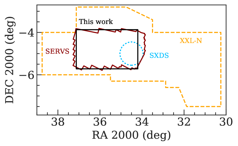
Figure 1: Illustration of the survey regions of XMM-XXL-North (XXL-N, Pierre et al. 2016, orange dashed line), the Subaru XMM-Newton Deep Survey (SXDS, Ueda et al. 2008, blue dotted circle), and the XMM-SERVS survey of XMM-LSS presented in this work (black box). The Spitzer SERVS coverage of XMM-LSS is also shown as the red polygon.

2 XMM-Newton Observations in the XMM-LSS region and data reduction

Table 2: The XMM-Newton data used to create the source catalog include 155 pointings with a total of 2.7 Ms of flare-filtered exposure time, of which 1.1 Ms is from the new AO-15 observations.^a Columns from left to right: target field, XMM-Newton revolution, XMM-Newton ObsID, observation starting date/time, Right Ascension and Declination of the pointing center (J2000, degrees), cleaned exposure time for PN, MOS1, and MOS2 in each pointing. This table is available in its entirety online.

Field	Revolution	ObsID	Date	R.A.	Decl.	GTI (PN)	GTI (MOS1)	GTI (MOS2)
			(UT)			(ks)	(ks)	(ks)
AO-15	3054	0780450101	2016-08-13T01:34:06	35.81072	$-5.15989$	20.91	23.61	23.61
XMM-LSS	1205	0404965101	2006-07-09T08:08:08	35.80953	$-5.48532$	3.44	10.36	9.91
XMDS	287	0111110401	2001-07-03T14:01:54	35.97582	$-5.15253$	21.40	27.20	27.40
SXDS	118	0112370101	2000-07-31T21:57:54	34.47819	$-4.98115$	39.13	42.70	42.83
XMM-XXL-North	2137	0677580101	2011-08-10T01:53:35	37.16867	$-4.49993$	4.94	5.93	5.52
XMM-XXL-North	2137	0677580101	2011-08-10T01:53:35	37.33404	$-4.49993$	2.01	6.47	6.67
XLSSJ022404.0–041328	0928	0210490101	2005-01-01T19:08:30	36.03267	$-4.20230$	80.28	87.98	87.98

^a: MOS only (MOS1 and MOS2 have the same exposure time). For PN, the total flare-filtered time is 2.3 Ms, of which 0.9 Ms is from the new AO-15 observations.

2.1 XMM-Newton and Chandra data in the XMM-LSS region

The XMM-LSS field has been targeted by a number of XMM-Newton surveys of different sensitivities (e.g., see Fig. 3 of Brandt & Alexander 2015 and Fig. 1 of Xue 2017). The original XMM-LSS survey was an $\approx 11$ deg² field typically covered by XMM-Newton observations of $\approx 10$ ks exposure time per pointing (Pacaud et al., 2006; Pierre et al., 2016). Within the 11 deg² field, $\approx 4$ deg² were observed by the XMM-Newton Medium Deep Survey (XMDS, $20-25$ ks exposure depth, Chiappetti et al., 2005). In addition, the Subaru XMM-Newton Deep Survey (SXDS, Ueda et al., 2008), adjacent to the XMDS field, covers a 1.14 deg² area and reaches a nominal $\approx 50$ ks exposure per pointing (Ueda et al., 2008). Moreover, the XMM-LSS field recently became a part of the 25 deg² XMM-XXL-North field (Pierre et al., 2016), which has similar XMM-Newton coverage as the original XMM-LSS survey (i.e., $\approx 10$ ks depth).

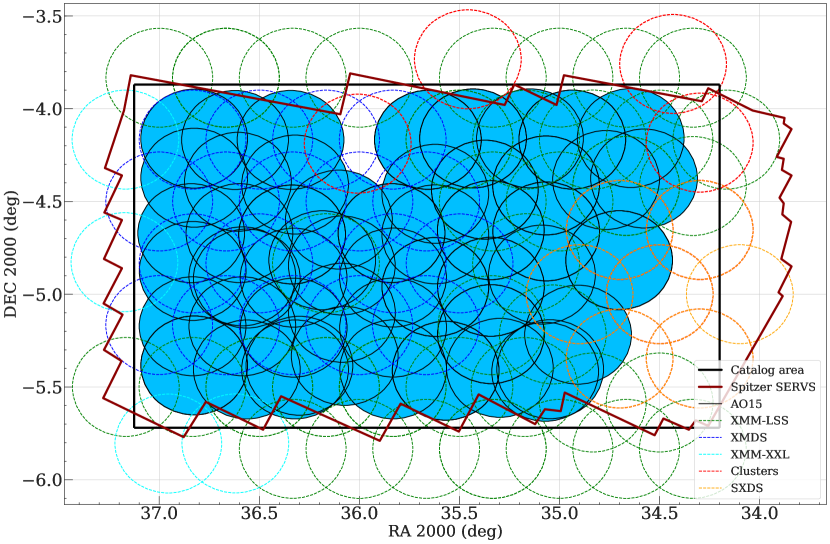
Figure 2: Locations of the XMM-Newton observations used in this work. The AO-15 observations are marked as the blue-filled circles with solid boundaries. The archival observations are marked as dashed circles. Circles with green, orange, blue, and cyan colors are for XMM-LSS, SXDS, XMDS, and XMM-XXL observations, respectively. The RA/DEC range of our catalog selection area is indicated by the black rectangle, and the Spitzer SERVS footprint is marked as the dark-red polygon. Our AO-15 observations do not cover the entirety of the SERVS region, because the existing data from SXDS (bottom-right corner, orange circles) and from deep X-ray cluster observations (top-middle and top-right, the red circles) reached the desired depth.

In addition to the XMM-Newton data, the XMM-LSS region has extensive multiwavelength coverage (see Table 1 for a summary, also see Vaccari 2016). In particular, the central $\approx 5$ deg² area of the XMM-XXL-North field (i.e., the combination of the XMDS and SXDS fields, see Fig. 1 for an illustration of the relative positions of different surveys.) was selected to be one of the SERVS fields. This sky region is covered uniformly by multiple photometric and spectroscopic surveys (see Sec. 4 for more details), and it is one of the deep drilling fields of the Dark Energy Survey (Diehl et al., 2014) and the upcoming Large Synoptic Survey Telescope (LSST) surveys (see Table 1). However, compared to the relatively uniform multiwavelength data, archival XMM-Newton observations covering this sky region span a wide range of exposure time (see Table 2). In order to advance studies of accreting SMBHs and their environments, deep X-ray observations with similar areal coverage are required in addition to the rich multiwavelength data in this field. To this end, we obtained XMM-Newton AO-15 observations taken between July 2016 and February 2017 with a total of 1.3 Ms exposure time. The relative sky coverage of our survey region, XMM-XXL-North, and SXDS are displayed in Fig 1. Our AO-15 data include 67 XMM-Newton observations. All of these 67 observations were carried out with a THIN filter for the EPIC cameras. The choice of the THIN filter maximizes the signal-to-noise ratio. Since the XMM-LSS field is far from the Galactic plane and thus the number of bright stars is small, the optical loading effects are negligible for almost all detected X-ray sources. Even for the brightest star in XMM-LSS, HD 14417, the optical loading effects are only limited to a few pixels at its position. In addition to the new data, we made use of all the overlapping archival XMM-Newton observations to create a uniform, sensitive XMM-Newton survey contiguously covering most of the SERVS data in the XMM-LSS region. After excluding observations that were completely lost due to flaring background (see §2.2), the archival data used here include 51 observations culled from the $10$ ks XMM-LSS survey, 18 observations from XMDS with $20-25$ ks exposures, four mosaic-mode observations obtained as part of the XMM-XXL survey (Pierre et al., 2016), four archival XMM-Newton observations targeting galaxy clusters identified in the XMM-XXL-North and XMM-LSS surveys ($\approx 30-100$ ks), and the ten $50$ ks observations from SXDS. We present the details of each observation in Table 2, and show the positions of each XMM-Newton observation used in this work in Fig. 2.

Our AO-15 observations were separated into two epochs to minimize the effects of background flaring. We first observed the XMM-LSS sky region in the SERVS footprint with $\approx 1$ Ms of XMM-Newton exposure time during July–August 2016. These first observations were screened for flaring backgrounds (§2.2); we then re-observed the background-contaminated sky regions using the remaining 0.3 Ms. We also observed the SXDS region in which one of the SXDS observations carried out in 2002 was severely affected by background flares. In this work, we present an X-ray source catalog obtained from a 5.3 deg² sky-region with $34.2^{\circ}\leq\alpha_{\rm J2000}\leq 37.125^{\circ}$ and $-5.72^{\circ}\leq\delta_{\rm J2000}\leq-3.87^{\circ}$ (black rectangle in Fig 1 and Fig 2). The sky region is primarily selected by the footprint of our AO-15 observations, with additional SXDS data within the SERVS footprint in the south-west corner. A total of $3.0$ Ms of raw XMM-Newton observations are used for generating the X-ray source catalog.

In addition to the XMM-Newton data, there are also a number of Chandra observations in our source-search region, including 18 observations of 10–90 ks exposure depth following up X-ray galaxy clusters identified in the XMM-LSS and XMM-XXL surveys (PIs: Andreon, S.; Jones, L.; Mantz, A.; Maughan, B.; Murray, S.; Pierre, M.); these observations occupy a wide RA/DEC range in our catalog region. In §4.1 and §4.2, we make use of the Chandra sources in these observations culled from the Chandra Source Catalog 2.0 (CSC 2.0; Evans et al., 2010). There are a total of 328 Chandra sources from CSC 2.0 in our survey region. Note that the source-flux information is not yet available for the CSC 2.0 Preliminary Detections List. Of these 328 Chandra sources, 201 of them are in CSC 1.1 (Evans et al., 2010). Their 0.5–7 keV band fluxes range from $3\times 10^{-16}-1.7\times 10^{-13}$ erg cm^-2 s^-1, with a median value of $9.7\times 10^{-15}$ erg cm^-2 s^-1. We use these Chandra sources as a means to improve and assess the multiwavelength counterpart identification reliabilities, since Chandra has better angular resolution and astrometric accuracy than those of XMM-Newton.

2.2 Data preparation and background-flare filtering

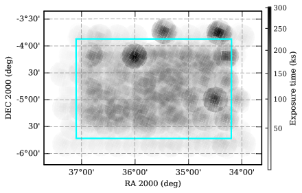
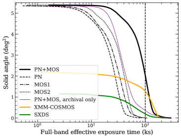
Figure 3: Left – Full-band survey effective exposure map (PN + MOS). The 5.3 deg² survey region from which the X-ray source catalog is constructed is marked as the cyan rectangular box. Except for several regions with deep XMM-Newton follow-up observations of galaxy clusters, the XMM-Newton coverage in our survey region is generally uniform. Right – The black solid line shows the cumulative survey solid angle as a function of full-band effective (i.e., vignetted) PN+MOS exposure for observations used in this work. Distributions for individual instruments are indicated as the dashed line (PN), dash-dotted line (MOS1), and dotted line (MOS2). For comparison, the cumulative survey solid angle for the archival XMM-Newton data in our survey region, in XMM-COSMOS, and in SXDS are shown as the thin purple line, thick orange line, and thick green line, respectively. The dashed vertical line marks exposure time $=100$ ks.

We use the XMM-Newton Science Analysis System (SAS) 16.1.0 and HEASOFT 6.21 for our data analysis. The XMM-Newton Observation Data Files (ODFs) were processed with the SAS tasks epicproc (epproc and emproc for PN and MOS, respectively) to create MOS1, MOS2, PN, and PN out-of-time (OOT) event files for each ObsID. For observations taken in mosaic mode or with unexpected interruptions due to strong background flares, we use the SAS task emosaic_prep to separate the event files into individual pseudo-exposures and assign pseudo-exposure IDs. For the mosaic-mode observations, we also determine the sky coordinates of each pseudo-exposure using the AHFRA and AHFDEC values in the attitude files created using the SAS task atthkgen.

For each event file, we create single-event light curves in time bins of 100 s for high (10–12 keV) and low (0.3–10 keV) energies using evselect to search for time intervals without significant background flares (the “good time intervals”, GTIs). We first remove time intervals with 10–12 keV count rates exceeding $3\sigma$ above the mean, and then repeat the $3\sigma$ clipping procedure for the low-energy light curves. Since background flares usually manifest themselves as a high-count-rate tail in addition to the Gaussian-shape count-rate histogram, adopting the $3\sigma$ clipping rule can effectively remove the high-count-rate tail while retaining useful scientific data. For a small number of event files with intense background flares, we filter the event files using the nominal count-rate thresholds suggested by the XMM-Newton Science Operations Centre. We exclude 12 pointings with GTI $<$ $2$ ks from our analysis. A total of 2.7 Ms (2.3 Ms) of MOS (PN) exposure remains after flare filtering, including 1.1 Ms (0.9 Ms) from AO–15 and 1.6 Ms (1.4 Ms) from the archival data. The flare-filtered median PN exposure time of the full 5.3 deg² survey region is $\approx 45.8$ ks. For the central $\approx 4.5$ deg² region covered by SERVS, the median PN exposure time is $48.5$ ks. These values were not corrected for vignetting.

After screening for background flares, we further exclude events in energy ranges that overlap with the instrumental background lines (Al K$\alpha$ lines at 1.45–1.54 keV for MOS and PN, which usually accounts for $\approx 10\%$ of the mean counts; Cu lines at 7.2–7.6 keV and 7.8–8.2 keV for PN, which accounts for 30% of the 2–10 keV counts).

From the flare-filtered, instrumental-line-removed event files, we construct images with a commonly adopted $4^{\prime\prime}$ pixel size using evselect in the following bands: 0.5–2 keV (soft), 2–10 keV (hard), and 0.5–10 keV (full). For each image, we generate exposure maps with and without vignetting corrections using the SAS task eexpmap. We set usefastpixelization=0 and attrebin=0.5 in order to obtain more accurate exposure maps. The exposure maps without vignetting-corrections are only used for generating maps of the instrumental background, which is not affected by vignetting (see §3). Detector masks were also generated using the SAS task emask. The distribution of vignetting-corrected exposure values across the XMM-LSS field and the PN+MOS1+MOS2 exposure map are presented in Fig. 3.

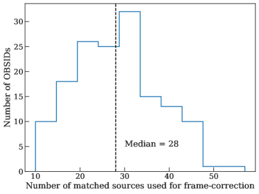
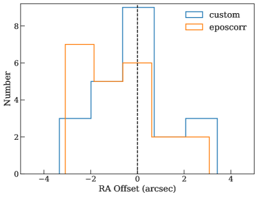
Figure 4: Left: Distribution of the number of X-ray sources used for finding the required angular offset. The median value is marked as the dashed line. Right: Distributions of optical-to-X-ray separations in RA for the matched X-ray sources in ObsID 0037982201 after the astrometric corrections. The results based on our iterative method are shown as the blue histogram, and the results based on the eposcorr task are shown as the orange histogram. For the vast majority of the ObsIDs, the difference is small, but some have non-negligible differences and we choose the required astrometric correction based on comparing angular-offset distributions similar to the one shown here.

3 The Main X-ray Source Catalog

3.1 First-pass source detection and astrometric correction

The astrometric accuracy of XMM-Newton observations can be affected by the pointing uncertainties of XMM-Newton. This uncertainty is usually smaller than a few arcsec, but can be as large as $\approx 10^{\prime\prime}$ (e.g., Cappelluti et al., 2007; Watson et al., 2008; Rosen et al., 2016). To achieve better astrometric accuracy and to minimize any systematic offsets between different XMM-Newton observations, we run an initial pass of source detection for each observation and then use the first-pass source list to register the XMM-Newton observations onto a common WCS frame. The first-pass source detection methods are outlined below:

1. For the exposures taken by each of the three instruments for each observation, we generate a temporary source list using the SAS task ewavelet with a low likelihood threshold (threshold=4). ewavelet is a wavelet-based algorithm that runs on the count-rate image generated using the image and vignetting-corrected exposure map extracted as described in §2.2.

   

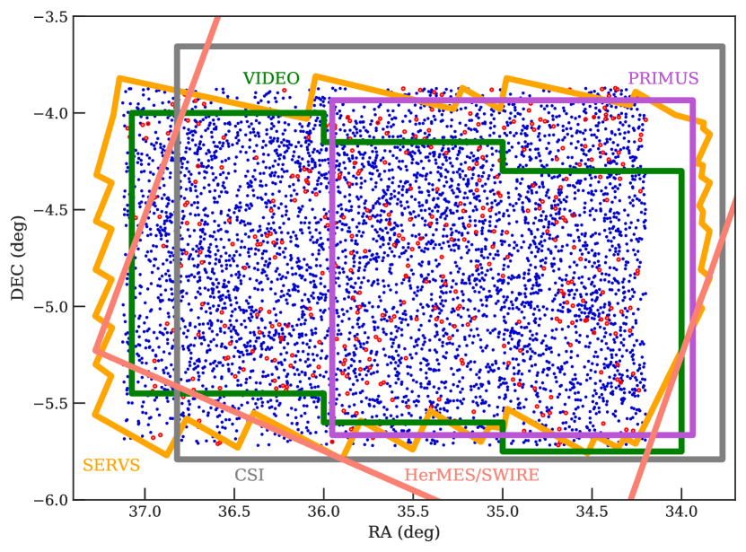
   Figure 5: Spatial distribution of the 5242 sources detected in this work. We have identified reliable multiwavelength counterparts (see Sec. 4.1 and Sec. 4.2 for details) for 93% of the XMM-Newton sources (blue dots), while the remaining 7% of sources are marked as open red circles. Some of the multiwavelength coverage of the XMM-LSS field is also shown as labeled (see §4 for details).

2. We use the temporary source list as an input to generate background images using the SAS task esplinemap with method=model. This option fits the source-excised image with two templates: the vignetted exposure map, and the un-vignetted exposure map. The former represents the cosmic X-ray background with an astrophysical origin, while the latter represents the intrinsic instrumental noise. esplinemap then finds the best-fit linear combination of the two templates and generates a background map. The details of this method are described in Cappelluti et al. (2007). The background maps are used for the PSF-fitting based source detection task described in Step (iv).

3. We run ewavelet again for each observation. This time the source list is generated by running ewavelet on the exposure map and image coadded across the PN, MOS1, and MOS2 exposures (when available) with the default likelihood threshold (threshold=5).

4. For each ewavelet source list, we use the SAS task emldetect to re-assess the detection likelihood and determine the best-fit X-ray positions. emldetect is a PSF-fitting tool which performs maximum-likelihood fits to the input source considering the XMM-Newton PSF, exposure values, and background levels of the input source on each image. emldetect also convolves the PSF with a $\beta$-model brightness profile for clusters and uses the result to determine if the input source is extended. Instead of running on the co-added image, emldetect takes the image, exposure map, background map, and detector mask of each input observation into account. We use a stringent likelihood threshold (likmin$=10.8$) to ensure that astrometric corrections are calculated based on real detections, and we only keep the point sources.

5. For the mosaic-mode observations (see Footnote 2), the multiple pointings under the same ObsID were already registered on the same WCS frame of the ObsID. Therefore, we do not correct the astrometry for each pseudo-exposure but only consider the astrometric offsets on an ObsID-by-ObsID basis. The source lists for the mosaic-mode observations were generated using the SAS task emosaic_proc, which is a mosaic-mode wrapper for procedures similar to (i)-(iv) described above.

For steps (iv) and (v), the source searching was conducted simultaneously on the images of the three EPIC cameras as the astrometric offsets between PN, MOS1, and MOS2 are negligible. For each ObsID, we cross-correlate the high-confidence emldetect list of point sources (with the emldetect flag EXT$=0$) with the optical source catalog culled from the Hyper Suprime-Cam Subaru Strategic Program Public Data Release 1 (HSC-SSP; Aihara et al., 2018), which is an ultra-deep optical photometric catalog with sub-arcsec angular resolution. The astrometry of HSC-SSP is calibrated to the Pan-STARRS1 $3\pi$ survey and has a $\lesssim 0.05^{\prime\prime}$ astrometric uncertainty. More details of the HSC-SSP catalog can be found in Aihara et al. (2018), and it is also briefly discussed in §4. For astrometric corrections, we limit the optical catalog to HSC sources with $i=18-23$ to minimize possible spurious matches due to large faint source densities at $i>23$ and matches to bright stars that might have proper motions or parallaxes.

The offset between each ObsID and the HSC catalog is calculated based on a maximum-likelihood algorithm similar to the SAS task eposcorr. The major difference between our approach and eposcorr is that we use an iterative optimization approach compared to the grid-searching algorithm adopted by eposcorr. During each iteration, we cross-correlate the optical catalog with the X-ray catalog using a $10^{\prime\prime}$ search radius and exclude all matches with multiple counterparts (less than $5\%$ of our X-ray sources have more than one optical counterpart in the bright HSC-SSP catalog). The $10^{\prime\prime}$ search radius is motivated by both the positional accuracy and PSF size of XMM-Newton, and the largest separations between the XMM-Newton and Chandra positions of the sources in the Chandra COSMOS Legacy Survey (Marchesi et al., 2016). We then calculate the required astrometric corrections that maximize the cross-correlation likelihood. After each iteration, we apply the best-fit astrometric offsets to the source list and next repeat the catalog cross-correlation steps and re-calculate the required additional corrections for the source list. The required astrometric corrections usually converge after 1–2 iterations. For the purpose of frame correction, we adopt the X-ray positional uncertainties calculated based on the PSF-fitting likelihood ratios provided by emldetect ($\sigma_{eml}$ hereafter). The positional uncertainty information is necessary because the required astrometric corrections should be weighted toward X-ray sources with better positions within each observation. To avoid over-weighting sources with extremely small $\sigma_{eml}$, we also include a constant $0.5^{\prime\prime}$ systematic uncertainty when calculating the best-fit values for frame-correction. The median number of X-ray sources in an ObsID with only one HSC counterpart within $3^{\prime\prime}$ is 28. See Fig. 4-left for a histogram of the number of X-ray sources used for determining the required angular offsets.

The required frame-correction offsets calculated using our approach are less than $3^{\prime\prime}$ in both RA and DEC and are generally consistent with the results calculated using eposcorr, with a median difference of $0.1^{\prime\prime}$. For demonstration purposes, we show the difference between our RA offsets and the eposcorr RA offsets for ObsID 0037982201 in Fig 4-right. For two ObsIDs the difference between our offsets and the eposcorr offsets are non-negligible ($>0.5^{\prime\prime}$). We visually inspect the X-ray to optical angular offsets similar to the one shown in Fig 4-right of these ObsIDs and conclude that our approach does improve the alignments between the optical and corrected X-ray images. The event files and the attitude file for each ObsID are then projected onto the WCS frame of the HSC catalog by updating the relevant keywords using a modified version of Chandra’s align_evt routine (Ranalli et al., 2013). Since the sky coordinates for the event files of the mosaic-mode pseudo-pointings are derived based on the reference point centered at the nominal RA and DEC positions of the mosaic-mode ObsIDs, we also recalculate the sky coordinates for these event files with the SAS task attcalc using the true pointing positions as the reference point, which is necessary for using regular SAS tasks for mosaic-mode pseudo-exposures.

3.2 Second-pass source detection

We re-create images, exposure maps, detector masks, and background maps using the frame-corrected event files and attitude files. We then run source-detection tasks for the second time considering all XMM-Newton observations listed in Table 2. Similar to the approach used for the XMM-H-ATLAS survey (Ranalli et al., 2015), we divide the XMM-LSS field into a grid when running the second-pass source detection because the number of images that can be processed by a single emldetect thread is limited. We use a custom-built wrapper of relevant SAS tasks to carry out the second-pass source detection, which is similar to the griddetect tool built for the XMM-H-ATLAS survey (Ranalli et al., 2015).

The cell sizes of the grid are determined by the number of ewavelet sources. For each cell in the grid, we co-add the images and exposure maps for all observations with footprint inside the cell and run ewavelet with a low detection threshold on the co-added image and exposure map. For each cell, we only keep ewavelet sources within the RA/DEC range of the cell plus 1^′ “padding” on each side of the cell. We then use the ewavelet list as an input for emldetect to assess the detection likelihood. The emldetect point-source list of the full XMM-LSS region is constructed from the union of the sources from all cells after removing duplicates due to the “padding”. We search for sources in three different bands: 0.5–2 keV (soft), 2–10 keV (hard), and 0.5–10 keV (full). For each source, emldetect computes a detection likelihood det_ml, which is defined as det_ml$=-\ln P$, where $P$ is the probability of a detected source being a random Poisson fluctuation of the background. In practice, the spurious fractions of a source catalog derived based on simulations are known to differ from the values obtained with the simple det_ml$=-\ln P$ equation (e.g., Cappelluti et al., 2007, 2009; Ueda et al., 2008; Watson et al., 2008; LaMassa et al., 2016). Since the source catalog is constructed based on a complex multi-stage source-detection approach, the relation between det_ml and the true spurious fraction may not be as straightforward as the simple det_ml$=-\ln P$ equation, especially in the low source count regime where even this simple relation fails. Therefore, we do not adopt a single det_ml value for our source catalog. Instead, we use the det_ml value corresponding to the 1% spurious fraction determined by simulations for each band (see the next subsection, §3.3, for details). The det_ml thresholds with 1% spurious fraction are 4.8, 7.8, and 6.2 for the soft, hard, and full bands, respectively. A total of 5242 sources satisfy this criterion in at least one of the three bands (see §3.5). We show the spatial distribution of the 5242 detected sources in Fig. 5.

3.3 Monte Carlo simulations

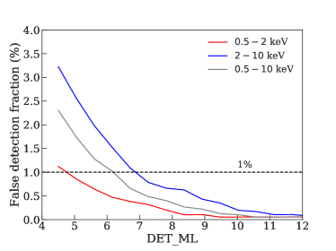
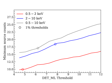
Figure 6: Left: The fraction of spurious sources detected at different det_ml based on simulations. The detection threshold relevant to our catalog is marked as the horizontal dashed line. Right: The minimum source counts for the detected sources (the median of all 20 simulations) with det_ml values above a given det_ml threshold. As expected, higher det_ml thresholds can only detect sources with higher numbers of counts. The det_ml values corresponding to the $1\%$ spurious fraction are marked as the open circles.

To assess our survey sensitivity and catalog reliability, we perform Monte Carlo simulations of X-ray observations. For each simulation, we generate a list of mock X-ray sources by sampling from the $\log N-\log S$ relations reported in the XMM-COSMOS survey (Cappelluti et al., 2009, for the 0.5–2 keV and 2–10 keV bands) and the Chandra Multiwavelength Project survey (ChaMP; Kim et al., 2007, for the 0.5–10 keV band). The maximum flux of the mock X-ray catalogs is set at $10^{-11}$ erg cm^-2 s^-1. The minimum flux of the mock X-ray sources at each energy band is set as 0.5 dex lower than the minimum detected flux (e.g., LaMassa et al., 2016). We randomly place the mock X-ray sources in the RA/DEC range covered by the XMM-Newton observations used in this work. We then use a modified version of the simulator written for the XMM-Newton survey of the CDF-S (Ranalli et al., 2013), CDFS-SIM, to create mock event files. CDFS-SIM converts X-ray fluxes to PN and MOS count rates with the same model used for deriving the ECFs, and it then randomly places X-ray events around the source location according to the count rates, the XMM-Newton PSFs at the given off-axis angle, and the real exposure maps. We extract images from the simulated event files using the same methods described in §3. For each observation, the simulated image is combined with a simulated background, which is created by re-sampling the original background map according to Poisson distributions to create simulated images that mimic the real observations. For each energy band, a total of 20 simulations are created. We run the same two-stage source-detection procedures described in §3.2 on the simulated data products. For each simulation, we match the detected sources to the input sources within a $10^{\prime\prime}$ cut-off radius by minimizing the quantity $R^{2}$ (Eq. 4 of Cappelluti et al., 2009):

$$R^{2}=\big{(}\frac{\Delta{\rm RA}}{\sigma_{\rm RA}}\big{)}^{2}+\big{(}\frac{\Delta{\rm DEC}}{\sigma_{\rm DEC}}\big{)}^{2}+\big{(}\frac{\Delta{\rm RATE}}{\sigma_{\rm RATE}}\big{)}^{2}.$$ (1)

Here $\Delta{\rm RA}$ and $\Delta{\rm DEC}$ are the differences between the simulated RA/DEC positions and the RA/DEC positions obtained by running source detection on the simulated images. $\Delta{\rm RATE}$ is the difference between the simulated count rates and the detected count rates. $\sigma_{\rm RA}$, $\sigma_{\rm DEC}$, and $\sigma_{\rm RATE}$ are the uncertainties of RA, DEC, and count rates of the detected sources. Minimizing $R^{2}$ takes into account the flux and positional differences between the input catalog and the sources detected in the simulated images (e.g., Cappelluti et al., 2007; Ranalli et al., 2015). Detected sources without any input sources within the $10^{\prime\prime}$ radius are considered to be spurious detections.

Fig. 6-left presents the spurious fraction ($f_{\rm spurious}$) as a function of det_ml for the soft, hard, and full bands. For our catalog, we consider sources with $f_{\rm spurious}$ less than 1% to be reliably detected. At this threshold, the corresponding det_ml values are 4.8, 7.8, and 6.2 for the soft, hard, and full bands, respectively. The difference between the det_ml thresholds in the three bands are likely due to their different background levels. For the full X-ray source catalog of 5242 sources, the $f_{\rm spurious}=1\%$ criterion translates to $\approx 52$ spurious detections. For each source, we have also calculated a detection reliability parameter (defined as $1-f_{\rm spurious}$) for each band using the simulation results presented in Fig. 6-left, which can be used for selecting sources with a desired reliability. We also display the minimum detected source counts (the median values of all 20 simulations) as a function of the det_ml threshold in Fig.6-right. We test for source confusion following the methods described in Hasinger et al. (1998) and Cappelluti et al. (2007). For all the simulated sources that are detected (i.e., having det_ml values greater than the 1% thresholds), we consider sources with observed fluxes ($S_{\rm out}$) that are larger than the simulated fluxes ($S_{\rm in}$) by the following threshold to be “confused” sources: $S_{\rm out}/(S_{\rm in}+3\times S_{\rm out}^{\rm Err})>1.5$. Here $S_{\rm out}^{\rm Err}$ is the statistical fluctuation of the observed fluxes. The source confusion fractions are 0.14%, 0.16%, and 0.43% in the soft, hard, and full bands, respectively. For the 5242 X-ray sources in this catalog, these fractions translate to $\approx 7-22$ sources with confusion.

3.4 Astrometric accuracy

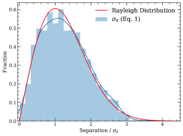
Figure 7: Histogram of the normalized full-band positional offsets, a dimensionless quantity defined as the positional offsets normalized by the empirically derived positional uncertainty, and comparison with the expected Rayleigh distribution, the solid red curve. The kernel-density estimation of the normalized positional offset distribution is shown as the solid blue curve. The excellent agreement between the two distributions suggests that our empirically derived $\sigma_{x}$ values are reliable indicators of the true positional uncertainties.

We investigate the positional accuracy of the XMM-Newton sources by comparing the second-pass X-ray catalog with the HSC-SSP catalog. Similar to the frame-correction procedures described in §3.1, we search for unique optical counterparts around the X-ray positions using a $3^{\prime\prime}$ search radius. For the 5199 X-ray sources detected in the full-band during the second-pass source-searching process, a total of 2434 X-ray sources are found to have only one $i=18-23$ HSC counterpart within $3^{\prime\prime}$. We use the separations between the optical and X-ray positions of this subsample as a means to determine empirical X-ray positional uncertainties, which is a commonly adopted practice in X-ray surveys (e.g. Watson et al., 2008; Luo et al., 2010; Xue et al., 2011, 2016; Luo et al., 2017).

The X-ray positional accuracy is determined by how well the PSF-centroid location can be measured, which usually depends on the number of counts of the detected source and the PSF size of the instrument (primarily dependent on the off-axis angle). For the vast majority of the X-ray sources presented in this work, the detected photons are from at least three different observations, and hence the dynamical range of effective off-axis angle for each source detected on the coadded image is relatively small. Thus, the X-ray positional uncertainty is mostly dependent on the number of counts available for detected sources. Using the angular separations between the 2434 X-ray sources and their unique optical counterparts, we derive an empirical relation between the number of X-ray counts, $C$, and the 68% positional-uncertainty radius ($r_{68\%}$) for the full-band-detected X-ray sources, $\log_{10}r_{68\%}=-0.31^{+0.02}_{-0.01}\times\log_{10}C+0.85$. The parameters are chosen such that $68\%$ of the sources have positional offsets smaller than the empirical relation.

For this work, we define the X-ray positional uncertainty, $\sigma_{x}$, to be the same as the uncertainties in RA and DEC where $\sigma_{\rm RA}=\sigma_{\rm DEC}=\sigma_{x}$. Under this definition, $\sigma_{x}$ is $r_{68\%}$ divided by a factor of $1.515$ (e.g., Eq. 21 and §4.2 of Pineau et al., 2017). The factor 1.515 is determined by integrating the Rayleigh distribution until the cumulative probability reaches 0.68. For reference, 90%, 95%, and 99.73% uncertainties correspond to $2.146\sigma_{x}$, $2.448\sigma_{x}$, and $3.439\sigma_{x}$, respectively. Because the separations in both RA and DEC behave as a univariate normal distribution with $\sigma_{\rm RA}$ and $\sigma_{\rm DEC}$, respectively, the angular separation should therefore follow the joint probability distribution function of the uncertainties in the RA and DEC directions. Since we assume $\sigma_{\rm RA}=\sigma_{\rm DEC}$, the angular separation between an optical source and an X-ray source should follow the univariate Rayleigh distribution with the scaling parameter $\sigma_{x}$, where $\sigma_{x}=\sigma_{\rm RA}=\sigma_{\rm DEC}$ (see §4 of Pineau et al., 2017, for details).

For each energy band, we repeat the same process to find the best-fit relation for $\sigma_{x}$ using the following equation:

$$\log_{10}\sigma_{x}=\alpha\times\log_{10}C+\beta.$$ (2)

Given the PSF size and positional accuracy of XMM-Newton, it is possible for X-ray sources to have angular separation from optical sources larger than $3^{\prime\prime}$, and the positional uncertainties derived based on counterparts found within the $3^{\prime\prime}$ search radius can be underestimated. Therefore, we adopt an iterative process. For each iteration, we use the derived $\sigma_{x}$ to identify reliable matches using the likelihood-ratio matching method described in §4.1. We then re-derive Eq. 2 using the reliable matches, and the updated astrometric uncertainties are used for running likelihood-ratio matching again. This is a stable process, as the parameters converge after 2–3 iterations. The average positional uncertainties ($\sigma_{x}$) for our soft-band, hard-band, and full-band X-ray catalogs are 1$\aas@@fstack{\prime\prime}$35, 1$\aas@@fstack{\prime\prime}$37, and 1$\aas@@fstack{\prime\prime}$31, respectively. The standard deviations of the positional uncertainties are 0$\aas@@fstack{\prime\prime}$37, 0$\aas@@fstack{\prime\prime}$25, and 0$\aas@@fstack{\prime\prime}$30 for the soft, hard, and full bands, respectively. Fig. 7 presents a comparison of the normalized separation (Separation/$\sigma$) between the full-band X-ray sources and their bright optical counterparts with $\sigma$ derived using Eq. 2, $\sigma_{x}$. The agreement between the Rayleigh distribution and the Separation/$\sigma_{x}$ distribution of our sample demonstrates that our empirically derived $\sigma_{x}$ values are reliable indicators of the true positional uncertainties. As for $\sigma_{eml}$, previous studies have reported that some on-axis sources with large numbers of counts can have unrealistically low $\sigma_{eml}$ values, therefore an irreducible systematic uncertainty should be added to $\sigma_{eml}$ for the normalized separation to follow a Rayleigh distribution (e.g., Watson et al., 2008), but the nature of this systematic uncertainty remains unclear. For this work, we use $\sigma_{x}$ as the positional uncertainties of our X-ray catalog, but $\sigma_{eml}$ is also included in the final catalog for completeness.

3.5 The main X-ray source catalog

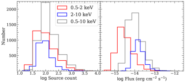
Figure 8: Left – Source-count distributions for the sources detected in the soft (red), hard (blue), and full (gray) bands. Right – Flux distributions of the sources detected in the three bands. Colors are the same as in the left panel.

We detect 3988, 2618, and 5199 point sources with $f_{\rm spurious}\leq 1\%$ in the 0.5–2 keV, 2–10 keV, and 0.5–10 keV bands, respectively. The details of the main X-ray source catalog are reported in Table F of Appendix A. The extended sources (identified by the EXT > 0 flag of emldetect) are not included, as the properties of the extended X-ray emission are beyond the scope of this work. We combine catalogs from the three energy bands using a similar approach to that adopted by the XMM-Newton Serendipitous Source Catalogue. We consider two sources from different catalogs to be the same if their angular separation is smaller than any of the following quantities: (1) 10^′′, (2) distance to the nearest-neighbor in each catalog, or (3) quadratic sum of the $99.73\%$ positional uncertainties from both bands. The final source catalog is the union of the sources detected in the three energy bands. We check for potential duplicate sources by visually inspecting all sources with distance to the nearest-neighbor (DIST_NN) less than 10^′′, and only one set of sources is found to be duplicated, resulting in a total of 5242 unique sources. There are 2967 sources with more than 100 PN+MOS counts in the full-band, and 126 sources with more than 1000 X-ray counts. A unique X-ray source ID is assigned to each of the 5242 sources at this stage. Visual inspection of the image in each band suggests that no apparent sources were missed by our detection algorithm.

We also derive the count rate (vignetting-corrected) to flux energy conversion factors (ECFs) assuming a power-law spectrum with photon index $\Gamma=1.7$, which is typical for distant X-ray AGNs found in XMM-Newton surveys with comparable sensitivities (e.g., XMM-COSMOS, Mainieri et al. 2007 and XMM-H-ATLAS, Ranalli et al. 2015) and Galactic absorption, $N_{\rm H}=3.57\times 10^{20}$ cm^-2. The energy ranges are those where the removed instrumental lines are excluded when deriving the ECFs. Since the archival observations and the AO-15 observations were carried out in different epochs between 2000–2017, we compute the ECFs by taking the slight temporal variations in the EPIC instrumental calibrations into account. In detail, we make use of the “canned” response files of 14 different epochs for MOS and 3 different epochs for PN available at the XMM-Newton SOC website. The effective ECF for each detected source is the exposure-time-weighed average of all relevant observations. For all X-ray sources, the mean conversion factors for (PN, MOS1, MOS2) are $(6.23,1.78,1.76)$, $(1.15,0.43,0.43)$, and $(2.84,0.88,0.87)$ counts s${}^{-1}/10^{-11}$erg cm^-2 s^-1, in the 0.5–2 keV, 2–10 keV, and 0.5–10 keV bands, respectively. We note that temporal variations in the ECFs are $<1\%$ for all three bands (e.g., Mateos et al., 2009; Rosen et al., 2016). For each source detected by emldetect, the flux from each EPIC camera is calculated separately using the corresponding ECF. The final flux of the source is the error-weighted mean of the fluxes from the three EPIC cameras, when available. The median fluxes for the soft, hard, and full bands are $2.9\times 10^{-15}$, $1.5\times 10^{-14}$, and $9.4\times 10^{-15}$ erg cm^-2 s^-1, respectively. The source-count and flux distributions of the sources detected in the three energy bands are displayed in Fig. 8.

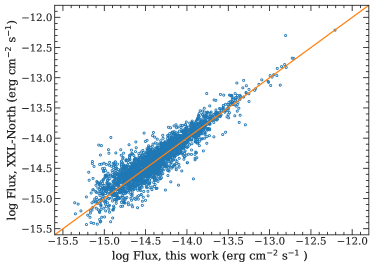
Figure 9: Comparison of the soft-band X-ray fluxes of our X-ray sources and those of the XMM-Newton counterparts identified in the XMM-XXL-North source catalogs (Liu et al., 2016) within a 10^′′ radius. As expected, almost all of the XMM-XXL-North X-ray sources in our catalog region can be matched to a counterpart in our X-ray source catalog with comparable flux.

For sources that are detected in fewer than three bands, we calculate the source-count upper limits using the mosaicked background map of the band in which the source is not detected. The mosaicked background map of each band is generated by summing the background maps from all individual observations (see §3.1). According to the Poisson probability set by the emldetect detection likelihood threshold ($P_{\rm Random}$, the probability of the detected source being a random Poisson fluctuation due to the background), we can calculate the minimum required total counts ($m$ in the following equation) required to exceed the expected number of background counts, $B$, using the regularized upper incomplete $\Gamma$ function (which is equivalent to Eq. 2 of Civano et al. 2016 if $m$ is a positive integer):

$$P_{\rm Random}=\frac{1}{\Gamma(m)}\int_{B}^{\infty}t^{m-1}e^{-t}dt$$ (3)

The upper limits are those corresponding to the det_ml values with a 1% spurious fraction: $P_{\rm Random}=8.2\times 10^{-3}$ for the soft band, $P_{\rm Random}=4.1\times 10^{-4}$ for the hard band, and $P_{\rm Random}=2.0\times 10^{-3}$ for the full band. For each non-detected source in each band, we determine the background counts by summing the background map within the circle with 70% encircled energy fraction (EEF). We then calculate $m$ by solving Eq. 3 using the Scipy function scipy.special.gammainccinv. Since $m$ is the required total counts to exceed random background fluctuations at the given probability, the flux upper limit is calculated based on the following equation, which is similar to Equation 2 of Cappelluti et al. (2009) and Equation 2 of Civano et al. (2016):

$$S=\frac{m-B}{t_{\rm exp}\times{\rm EEF}\times{\rm ECF}}.$$ (4)

Here EEF corrects for PSF loss and is 0.7, and $t_{\rm exp}$ is the median exposure time within the 70% EEF circle. The flux upper limits are calculated as the exposure-time-weighted mean of the three EPIC detectors.

For each source detected in either the soft or the hard band (or both), we calculate its hardness ratio (HR), defined as $(H-S)/(H+S)$, where $H$ and $S$ are the source counts weighted by the effective exposure times in the hard and the soft bands, respectively. The source counts are the default output of emldetect, which is the sum of the counts from all three EPIC detectors. The three EPIC detectors have different energy responses, and the hardness ratios reported here did not take these into account. We report this value in our catalog for direct comparison with previous XMM-Newton studies. The uncertainties on HR are calculated based on the count uncertainties from the output of emldetect using the error-propagation method described in §1.7.3 of Lyons (1991). For sources not detected in either the soft or the hard band, we calculate the limits of their HRs assuming each non-detection has net counts $=m-B$, where $m$ is the count upper limits calculated using Eq. 3 and $B$ is the background counts. The HR uncertainties for these sources are set to $-$99.

We also report the hardness ratios independently for PN, MOS1, and MOS2, calculated using the Bayesian Estimation of Hardness Ratios (BEHR) code (Park et al., 2006) assuming the recommended indices for the $\Gamma$-function priors (softidx$=1$ and hardidx$=1$). BEHR is designed to determine HRs for low-count sources in the regime of Poisson distributions. It also computes uncertainties using Markov chain Monte Carlo methods for sources including those with non-detections in either the soft or hard band. Since our sources are usually detected over multiple exposures, we scale the HRs by setting the softeff and hardeff parameters in BEHR to account for the effective exposure times using Eq. (6) of Georgakakis & Nandra (2011). Qualitatively, the BEHR hardness ratios for sources that are detected in both the soft and hard bands are consistent with those calculated using the simple approach described in the previous paragraph. For the sources with non-detections in either the soft or hard band, we quote the default 68% upper or lower bounds calculated with BEHR. As expected, these limits are almost always weaker than the HR limits obtained by assuming the non-detections have 99% source count upper limits given by Eq. 3.

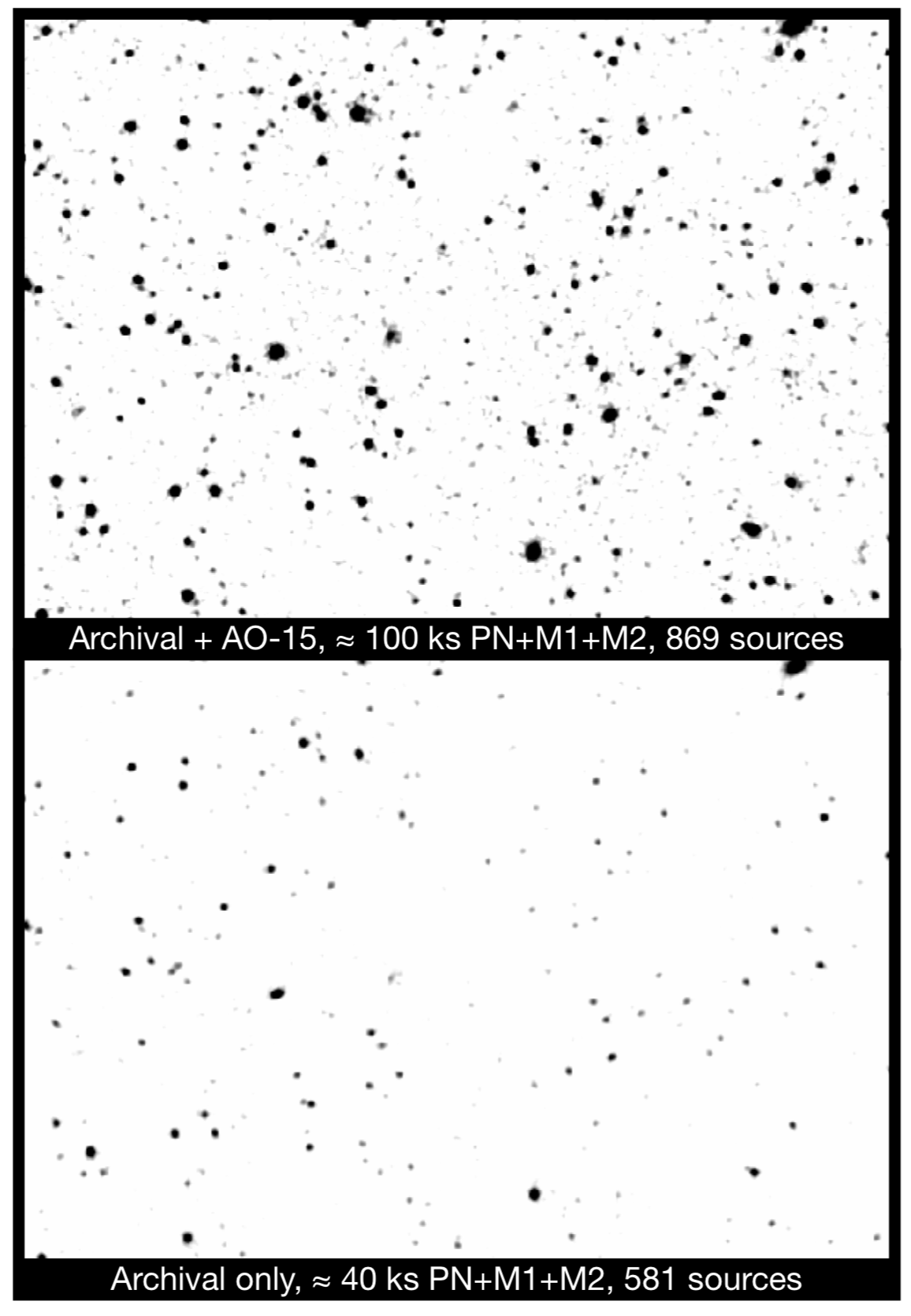
Figure 10: Top – Background-subtracted, smoothed, and coadded PN+MOS image in the 0.5–10 keV band for a $0.8\times 0.6$ deg² region centered at RA$=35.580^{\circ}$, DEC=$-4.965^{\circ}$. This image is created using both archival data and the new AO-15 data, and a total of 869 sources are detected in this region. Bottom – Same as the top image, but only the archival data are included. The two images are matched in color scale. In the Liu et al. (2016) catalog, only 581 sources can be found in this region. The typical vignetting-corrected exposure times are shown at the bottom of both panels. The exposure time of the full survey region is shown in Fig. 3.

As a comparison, a total of 2861 X-ray sources from XMM-XXL-North (Liu et al., 2016) are found to have a counterpart within the 10^′′ radius in our X-ray catalog. For these matched sources, we show a comparison between the soft-band X-ray fluxes reported in the XMM-XXL-North catalog and those in our catalog in Fig. 9. As expected, the majority of the archival sources detected in our catalog have archival soft-band fluxes consistent with those in our catalog. The small scatter in the measured fluxes is expected as the XMM-XXL-North catalog adopts a different source-detection method, background-subtraction approach, and energy conversion factors. Since the SXDS observations were also used for constructing the XXL-North (Liu et al., 2016) catalog, the 2861 sources matched to the XMM-XXL-North catalogs are considered to be matched to all available archival sources, and we conclude that the other 2381 X-ray sources in our catalogs are new sources. We include the IDs from the Liu et al. (2016) catalog for these matched sources in our catalog (Table F).

In our source-detection region, 172 sources from the original Liu et al. (2016) catalog do not have a counterpart in our point-source catalog. Of these 172 sources, 150 can be associated with extended sources or sources deemed unreliable based on our det_ml criteria (see §3.3). The remaining sources comprise $<1\%$ of the XMM-XXL-North catalog in our source-detection region. Visual inspection suggests that the vast majority of these sources might be spurious detections, but we cannot rule out the possibility that some sources are missed in our catalog due to X-ray variability (e.g., Yang et al., 2016; Falocco et al., 2017; Paolillo et al., 2017; Zheng et al., 2017). Also, the XMM-XXL-North catalog adopted a different source-detection approach (see §2 of Liu et al. 2016 for details). The properties of sources that exhibit strong X-ray variability will be presented in a separate work. Fig. 10 shows the background-subtracted, 0.5–10 keV PN+MOS image (see §3 for the details of the data analysis) from a $\approx 0.5$ deg² region in XMM-LSS generated using the combined AO-15 and archival data. An image produced using only the archival data is also displayed for comparison, demonstrating the improved source counts with the additional AO-15 observations.

Table 3: Sensitivity curves. Column 1: Soft-band flux. Column 2: Soft-band survey solid angle. Columns 3–4: Similar to Columns 1–2 but for the hard band. Columns 5–6: Similar to Columns 1–2 but for the full band. This table is available in its entirety online.

$\log S_{\rm 0.5-2keV}$	$\Omega_{\rm 0.5-2keV}$	$\log S_{\rm 2-10keV}$	$\Omega_{\rm 2-10keV}$	$\log S_{\rm 0.5-10keV}$	$\Omega_{\rm 0.5-10keV}$
(cgs)	(deg2)	(cgs)	(deg2)	(cgs)	(deg2)
(1)	(2)	(3)	(4)	(5)	(6)
$-$14.78	4.828	$-$13.93	4.652	$-$14.38	3.421
$-$14.77	4.862	$-$13.92	4.694	$-$14.37	3.583
$-$14.76	4.898	$-$13.91	4.737	$-$14.36	3.727
$-$14.75	4.931	$-$13.90	4.778	$-$14.35	3.855
$-$14.74	4.960	$-$13.89	4.815	$-$14.34	3.976
$-$14.73	4.991	$-$13.88	4.852	$-$14.33	4.081
$-$14.72	5.016	$-$13.87	4.885	$-$14.32	4.182
$-$14.71	5.044	$-$13.86	4.918	$-$14.31	4.262
…	…	…	…	…	…

3.6 Survey sensitivity, sky coverage, and $\log N-\log S$

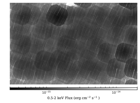
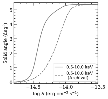
Figure 11: Left – Soft-band sensitivity map of the source-detection region (the same as the cyan box shown in Fig. 3). Right – Comparison of the full-band sky coverages between this work (solid line) and the archival XMM-Newton observations (dashed line), demonstrating the improved and more uniform sensitivity across the wide field enabled by the new data.

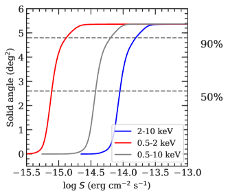
Figure 12: Sky coverage in the soft, hard, and full bands of our X-ray survey in XMM-LSS. The sensitivity curves were calculated with det_ml$=4.8$, 7.8, and 6.2 for the soft, hard, and full bands. These det_ml values correspond to $1\%$ spurious fraction based on extensive simulations (see §3.3.)

We create sensitivity maps of our survey region in different bands using the background and exposure maps generated as described in §2.2. The mosaicked background and exposure maps are binned to $5\times 5$ pixels ($20^{\prime\prime}\times 20^{\prime\prime}$). For each pixel of the binned, mosaicked background map, the minimum required source counts to exceed the random background fluctuations are calculated using Eq. 3. The sensitivity is then calculated using Eq. 4 with the corresponding EEF and ECF values. According the sensitivity maps, our survey has flux limits of $1.7\times 10^{-15}$, $1.3\times 10^{-14}$, and $6.5\times 10^{-15}$ erg cm^-2 s^-1 over 90% of its area in the soft, hard, and full bands, respectively, reaching the desired depth-area combination. We also compared the sensitivity maps with the detected sources, and find that the spatial distribution of the fluxes of our sources largely obey the sensitivity maps. The soft-band sensitivity map is presented in Fig. 11-left. We also generated a soft-band sensitivity map using only the archival data. To visualize the improvement upon the archival data, we compare the full-band sky coverage obtained from all available XMM-Newton data in our survey region with the sky coverage obtained using only the archival data. Fig. 11-right demonstrates the improved survey depth and uniformity with the new XMM-Newton observations. The sensitivity curves corresponding to the det_ml thresholds in the soft, hard, and full bands are shown in Fig. 12 and presented in Table 3.

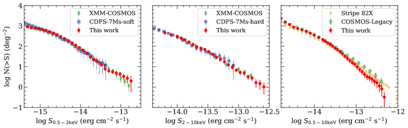
Figure 13: The $\log N-\log S$ relations for our catalog in the soft band (left), hard band (middle), and full band (right). For comparison, a few $\log N-\log S$ relations from surveys spanning a wide range of area and sensitivity are also shown (XMM-COSMOS, Cappelluti et al. 2009; Stripe-82X, LaMassa et al. 2016; COSMOS-Legacy, Civano et al. 2016; and CDF-S 7Ms, Luo et al. 2017; the energy range and power-law photon index differences have been corrected). The $\log N-\log S$ relations of our survey are generally consistent with those of previous studies.

We calculate the $\log N-\log S$ relations of our survey using the sky coverage curves described above and the following equation:

$$N(>S)=\sum\limits_{i=1}^{N_{s}}\frac{1}{\Omega_{i}}.$$ (5)

Here $N(>S)$ represents the total number of detected sources with fluxes larger than $S$, and $\Omega_{i}$ is the sky coverage associated with the flux of the $i$th source. The $\log N-\log S$ relations of our survey are shown in Fig. 13, along with the $\log N-\log S$ relations for a selection of surveys spanning a wide range of area and sensitivity (CDF-S 7Ms, Luo et al. 2017; XMM-COSMOS, Cappelluti et al. 2009; COSMOS-Legacy, Civano et al. 2016; and Stripe 82X, LaMassa et al. 2016). The flux differences caused by different choices of power-law indices and/or slight differences in energy ranges have been corrected assuming a $\Gamma=1.7$ power-law spectrum adopted in this work. Considering factors such as different spectral models and/or methods of generating survey sensitivity curves, our $\log N-\log S$ relations are consistent with the relations reported in the literature within the measurement uncertainties.

4 Multiwavelength counterpart identifications

The XMM-LSS region is one of the most extensively observed extragalactic fields. The publicly available multiwavelength observations in the XMM-LSS region utilized in this work are SERVS (Mauduit et al., 2012), SWIRE (Lonsdale et al., 2003), VIDEO (Jarvis et al., 2012), the CFHTLS-wide survey (Hudelot et al., 2012), and the HSC-SSP survey (Aihara et al., 2018).

We focus on identifying the correct counterparts for our X-ray sources in four deep optical-to-near-IR (OIR) catalogs: SERVS, VIDEO, CFHTLS, and HSC-SSP. SERVS is a post-cryogenic Spitzer IRAC survey in the near-IR 3.6 and 4.5 $\mu$m bands with $\approx 2\mu$Jy survey sensitivity limits and $\approx 5$ deg² solid-angle coverage in the XMM-LSS region. We make use of the highly reliable two-band SERVS catalog built using SExtractor, obtained from the Spitzer Data Fusion catalog (Vaccari, 2015), which has $\approx 4\times 10^{5}$ sources. The Spitzer Data Fusion catalog has already integrated data from SWIRE, which include photometry in all four IRAC bands and the photometry in MIPS 24, 70, and 160 $\mu$m. A total of $82\%$ of the X-ray sources have at least one SERVS counterpart candidate within their 99.73% positional-uncertainty radius ($r_{99\%}$ hereafter, which is equivalent to 3.44$\sigma_{x}$), which is calculated based on the quadratic sum of the 99.73% X-ray positional uncertainties and the corresponding OIR positional uncertainties.

VIDEO is a deep survey in the near-infrared Z, Y, J, H, and $K_{s}$ bands with $\approx 80\%$ completeness at $K_{s}<23.8$. In the XMM-LSS region, VIDEO covers a $4.5$ deg² area ($\approx 85\%$ of our X-ray survey region) with a total of $\approx 5.7\times 10^{5}$ sources; $79\%$ of the X-ray sources have at least one VIDEO counterpart candidate within $r_{99\%}$.

The CFHTLS-W1 survey covers the entirety of our X-ray data, with an $80\%$ completeness limit of $i^{\prime}=24.8$. We select the CFHTLS sources in the RA/DEC ranges marginally larger (1^′) than our source-detection region. We limit the CFHTLS sources to those with $SNR>5$ in the $i^{\prime}$-band. The total number of sources in the $i^{\prime}$-band selected catalog is $\approx 8.1\times 10^{5}$. A total of 90% of the X-ray sources in our catalog have at least one CFHTLS counterpart candidate within $r_{99\%}$.

The XMM-LSS field is entirely encompassed by the 108 deg² HSC-SSP wide survey. The limiting magnitude in the i-band for the wide HSC-SSP survey is 26.4. Inside the XMM-LSS field, HSC-SSP also has “ultra-deep” ($\approx 1.77$ deg²) and “deep” ($\approx 5$ deg²) surveys, which overlap with the SXDS and XMDS regions, respectively. We focus only on the wide survey because in the currently available data release it is only 0.1 mag shallower than the deep survey in the i-band, and the uniform coverage is important for determining the background source density when matching to the X-ray catalog (see §4.1). We select the i-band detected HSC-SSP sources in the RA/DEC ranges slightly larger than our source-detection region. The total number of HSC-SSP sources in our source-detection region is $\approx 3.1\times 10^{6}$, and $\approx 93\%$ of the X-ray sources in our main catalog have at least one HSC-SSP counterpart candidate within $r_{99\%}$.

Although CFHTLS is not as deep as HSC-SSP in the g, r, i, and z bands, it has complementary u^∗-band photometry. Including photometry from both optical surveys also ensures that we will minimize the risk of missing an optical counterpart due to bad photometry caused by artifacts such as satellite tracks in either survey.

Since there are small systematic offsets in the astrometry of each catalog, we match SERVS, VIDEO, and CFHTLS to the HSC-wide catalog, and correct for the small offsets between each catalog to the HSC-wide catalog to maximize the counterpart matching accuracy. In the RA direction, the adopted corrections are 0$\aas@@fstack{\prime\prime}$020, 0$\aas@@fstack{\prime\prime}$027, and 0$\aas@@fstack{\prime\prime}$026 for SERVS, VIDEO, and CFHTLS, respectively. For DEC, the adopted corrections are $-$0$\aas@@fstack{\prime\prime}$009, $-$0$\aas@@fstack{\prime\prime}$006, $-$0$\aas@@fstack{\prime\prime}$008 for SERVS, VIDEO, and CFHTLS, respectively.

4.1 The likelihood-ratio matching method

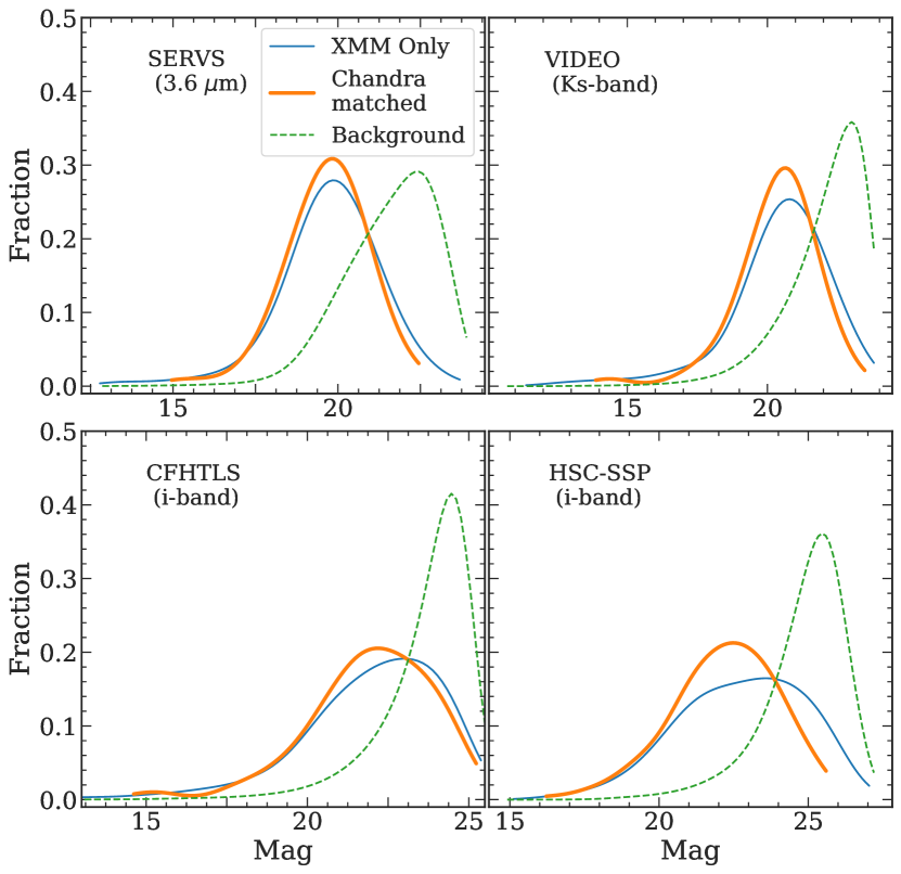
Figure 14: Kernel-density estimations of the magnitude distributions (solid lines) for the expected counterparts in SERVS (top-left), VIDEO (top-right), CFTHLS (bottom-left), and HSC-SSP (bottom-right). We show the distributions obtained using the full XMM-Newton catalog ($q(m)_{\it XMM-Newton}$), and the distributions obtained using the Chandra sources in the XMM-LSS field ($q(m)_{\it Chandra}$). The magnitude distributions of the background, unrelated sources are also displayed in each panel as the dashed curves. This figure demonstrates that $q(m)_{\it Chandra}$ significantly improves upon the background-dominated $q(m)_{\it XMM-Newton}$ for the deep OIR catalogs in the bottom panels (in particular, the most-probable magnitude values).

To match reliably the X-ray sources to the OIR catalogs with much higher source densities, we employ the likelihood-ratio method (LR hereafter) similar to previous X-ray surveys, (e.g., Brusa et al., 2007; Luo et al., 2010; Xue et al., 2011, 2016; Luo et al., 2017). The likelihood ratio is defined as the ratio between the probability that the source is the correct counterpart, and the probability that the source is an unrelated background object (Sutherland & Saunders, 1992):

$$LR=\frac{q(m)f(r)}{n(m)}.$$ (6)

Here $q(m)$ is the magnitude distribution of the expected counterparts in each OIR catalog, $f(r)$ is the probability distribution function of the angular separation between X-ray and OIR sources, and $n(m)$ is the magnitude distribution of the background sources in each OIR catalog.

We calculate the background source magnitude distributions using OIR sources between 10^′′ and 50^′′ from any sources in our X-ray catalog.

As discussed in §3.4, the probability distribution function of the angular separation should follow the Rayleigh distribution:

$$f(r)=\frac{r}{\sigma_{x}^{2}}\exp^{\frac{-r^{2}}{2\sigma_{x}^{2}}}.$$ (7)

Note that Eq. 7 is different from the two-dimensional Gaussian distribution function that maximizes at $r=0$, and thus the $LR$ values calculated in this work are not directly comparable to previous works that adopted a Gaussian $f(r)$.

In practice, for an X-ray source with a total of $Nc$ counterpart candidates within the search radius, the matching reliability for the $i$-th counterpart candidate $MR_{i}$, can be determined using the following equation:

$$MR_{i}=\frac{LR_{i}}{\sum_{k=0}^{N_{c}}LR_{k}+(1-Q)}$$ (8)

Here $Q$ is the completeness factor, which is defined as $Q=\int_{-\infty}^{m_{\rm lim}}q(m)$, where $m_{\rm lim}$ is the limiting magnitude of the OIR catalog being used for matching. For each counterpart candidate, $MR$ is equivalent to the relative matching probability among all possible counterpart candidates. See Eq. 5 of Sutherland & Saunders (1992) and §2.2 of Luo et al. (2010) for details.

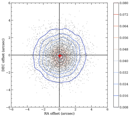
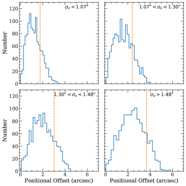
Figure 15: Left: Distribution of the OIR-to-X-ray positional offsets in the RA vs. DEC plane for the 4858 XMM-Newton sources with reliably matched OIR counterparts. The contours represent the isodensity levels of the points. The mean positional offsets are $<$ 0.1^′′ in both the RA and DEC directions (the red cross). Right: Histograms of positional offsets for the 4858 reliably matched sources, divided into four bins based on their positional uncertainties. In each panel, we also mark the median 68% positional offset value ($r_{\rm 68\%}$) as the vertical dashed line.

Due to the relatively large positional uncertainties of XMM-Newton and the high source densities of the OIR catalogs, deriving an accurate magnitude distribution of the expected counterparts, $q(m)$, using XMM-Newton data is challenging. Therefore, we obtain $q(m)$ for our X-ray sources by first matching our XMM-Newton catalog to the Chandra Source Catalog 2.0 (CSC 2.0; Evans et al., 2010) to take advantage of the higher angular resolution and positional accuracy of Chandra. We derive the positional uncertainties of the Chandra sources in our survey region using the same empirical approach described in Xue et al. (2011) by selecting CSC sources in the RA/DEC range of our catalog, and matching them onto HSC-SSP using a $1.5^{\prime\prime}$ radius. We select CSC sources that are uniquely matched to our X-ray catalogs within the $95\%$ uncertainties (Chandra and XMM-Newton positional uncertainties are added in quadrature). A total of 223 sources in our XMM-Newton catalog are matched to a unique Chandra source in the CSC. We match these Chandra sources to the four OIR catalogs using Eq. 6, with $q(m)$ derived using the iterative approach described in Luo et al. (2010), which determines the $LR$ threshold by optimizing the matching reliability and completeness. The $q(m)$ derived from the CSC sources, $q(m)_{\it Chandra}$, is then used as the expected magnitude distribution for OIR counterparts of our XMM-Newton sources. The X-ray flux distributions in the soft, hard, and full bands of the Chandra-matched subsample are similar to those of our entire XMM-Newton catalog, and therefore $q(m)_{\it Chandra}$ should be consistent with the intrinsic magnitude distributions of the real OIR counterparts of our full X-ray catalog. The counterpart-matching processes are run on four different OIR catalogs: SERVS, VIDEO, CFHTLS, and HSC-SSP. The details of the filters and apertures of the photometry in each OIR catalog can be found in Appendix A, where we give the descriptions of the columns reported in the source catalog (Columns 128–187 of Table F). For illustration, Fig. 14 shows the magnitude distributions of the background sources and the distributions of the expected counterparts derived using CSC sources.

For comparison, we also obtain $q(m)$ for the full XMM-Newton catalog without using the Chandra positions, $q(m)_{\it XMM-Newton}$. We again use the Luo et al. (2010) iterative method, but with a $3^{\prime\prime}$ initial search radius. $q(m)_{\it XMM-Newton}$ is also plotted in Fig. 14. It is evident that for ultra-deep OIR catalogs such as HSC-SSP and CFHTLS, $q(m)_{\it XMM-Newton}$ is skewed toward the faint background sources compared to the Chandra-matched subsample. For the other catalogs, we find no qualitative difference between $q(m)_{\it Chandra}$ and $q(m)_{\it XMM-Newton}$, but we still use $q(m)_{\it Chandra}$ for consistency.

We next compute the $LR$ values for all OIR sources within a 10^′′ radius (i.e., the counterpart “candidates”) of the X-ray sources using Eq. 6. For each OIR catalog, we choose the $LR$ thresholds ($LR_{\rm th}$) such that the reliability and completeness parameters are maximized (see Eq. 5 of Luo et al. 2010 for details). Counterparts with $LR>LR_{\rm th}$ are considered to be reliably matched. A summary of the results is reported in Table 4. For each OIR catalog, we list the number of all X-ray sources with at least one OIR counterpart candidate within $r_{99\%}$ of the X-ray sources, $N_{\rm All}$, and the number of X-ray sources with at least one reliably matched source with $LR>LR_{\rm th}$, $N_{\rm Reliable}$.

Table 4: Summary of $LR$ counterpart-matching results for each OIR catalog, with an additional summary row for the combined results from all OIR catalogs considered. The columns in the summary row are the same as those for individual OIR catalogs except for Column 7). Column 1: Catalog name. Column 2: Survey magnitude limit for each catalog in AB. Column 3: Survey area. Column 4: Positional uncertainty for each OIR catalog. Column 5: $LR$ threshold. Column 6: Total number of X-ray sources with at least one counterpart within the 10″ search radius in each catalog. Column 7: Average number of OIR sources within $r_{99\%}$ of the X-ray sources (if the X-ray source is within the coverage of the OIR catalog). Here the summary row shows the total number of X-ray sources with at least one OIR counterpart within $r_{99\%}$. Column 8: Total number of X-ray sources with at least one counterpart with $LR>LR_{\rm th}$. The summary row displays the number of all X-ray sources with at least one $LR>LR_{\rm th}$ counterpart from any of the four OIR catalogs, plus the 23 sources with only one unique counterpart within $r_{99\%}$ from all OIR catalogs considered (see §4.1 for details). X-ray sources having only one unique OIR counterpart in all OIR catalogs considered within $r_{99\%}$, but the $LR$ values do not exceed the reliability thresholds in all OIR catalogs. Columns 9–11: See §4.2 for details. Column 9: The fraction of X-ray sources in the “associated population” based on the results of Monte Carlo simulations. Column 10: False-matching rates determined using Monte Carlo simulations. Column 11: Fraction of the X-ray sources having identical reliable counterparts found based on their Chandra and XMM-Newton positions. Based on sources in regions where there is overlapping XMM-Newton and Chandra coverage. For the summary row, Columns 9–11 are calculated as the weighed sum (based on the number of primary counterparts from each catalog) of the results from all four OIR catalogs.

Catalog	Limiting Magnitude	Area	$\sigma$	$LR_{\rm th}$	$N_{\rm All}$	$\overline{N_{99\%}}$	$N_{\rm Reliable}$	$f_{\rm AP}$	False Rate	Identical Fraction
		deg2							(Simulation)	(Chandra)
(1)	(2)	(3)	(4)	(5)	(6)	(7)	(8)	(9)	(10)	(11)
SERVS	$3.6\mu$m $<23.1$	5.0	0.5″	0.32	4689	1.0	3948	96.8%	4.2%	97.3%
VIDEO	$Ks<23.8$	4.5	0.3″	0.25	4380	1.3	3827	86.3%	8.0%	94.4%
CFHTLS-wide	$i<24.8$	5.4	0.2″	0.22	5185	1.5	4207	75.6%	15.6%	90.8%
HSC-SSP	$i<26.5$	5.4	0.1″	0.25	5124	2.3	4317	78.6%	18.4%	87.3%
Summary	N/A	N/A	N/A	N/A	5237	5147	4858	93.1%	5.8%	97.1%

Motivated by the spurious-matching rates of different OIR catalogs (see §4.2 for the cross-matching reliability analysis), we first select a “primary” counterpart for each X-ray source from, in priority order, SERVS, VIDEO, CFHTLS, and HSC-SSP. After selecting the primary OIR counterpart, we associate different OIR catalogs with each other using a simple nearest-neighbor algorithm. Thanks to the much smaller positional uncertainties of the OIR catalogs, we adopt a constant search radius of 1^′′ for the OIR catalog associations, which is the approach used by the Spitzer Data Fusion database (Vaccari, 2015).

Using this approach, 4832 ($\approx 93\%$) X-ray sources have at least one robust counterpart with $LR>LR_{\rm th}$. We consider an additional 26 X-ray sources without any counterpart candidates having $LR>LR_{\rm th}$ to have “acceptable” matches because there is only one unique counterpart in all four OIR catalogs within $r_{\rm 99\%}$. When considering both the $LR>LR_{\rm th}$ counterparts and the acceptable counterparts, 4858 X-ray sources in our catalog are considered to have reliable OIR counterparts ($93\%$). Of these sources, 3968 are matched to SERVS as the primary counterpart, 367 are from VIDEO, 386 are from CFHTLS, and 137 are from HSC.

Besides the 4858 X-ray sources with reliable/acceptable counterparts, most of the remaining 384 sources have $f_{\rm spurious}\leq 0.05\%$ in at least one band, and thus they are unlikely to be spurious X-ray detections. 289 of these 384 sources still have at least one OIR counterpart candidate within the $r_{99\%}$ circle. Therefore, 5147 X-ray sources have at least one OIR counterpart candidate within $r_{\rm 99\%}$. Of the other 95 sources, 90 still have at least one OIR counterpart candidate within the $10^{\prime\prime}$ counterpart-searching radius. We still select counterparts for these sources and the properties of these counterparts are included in the main X-ray catalog. However, only the previously mentioned 4858 sources are considered to be reliably matched and are flagged in the catalog. We find 5 sources that are completely “isolated”, i.e., no counterpart candidates were found within a 10^′′ search radius. Visual inspection of these sources shows that all of them coincide with a bright star, thus making the pipeline OIR photometry unavailable.

Fig. 15 presents the positional offsets between the X-ray sources and the reliably matched sources. The small median positional offsets in the RA and DEC directions demonstrate the quality of our astrometry, and the histograms of the positional offsets for sources binned in different $\sigma_{x}$ show that our empirically derived positional uncertainties are reliable. For each source, we also generate postage-stamp images at X-ray, mid-IR, near-IR, and optical wavelengths. For illustration, we show a random collection of 16 X-ray sources with reliable counterparts in Fig. 16.

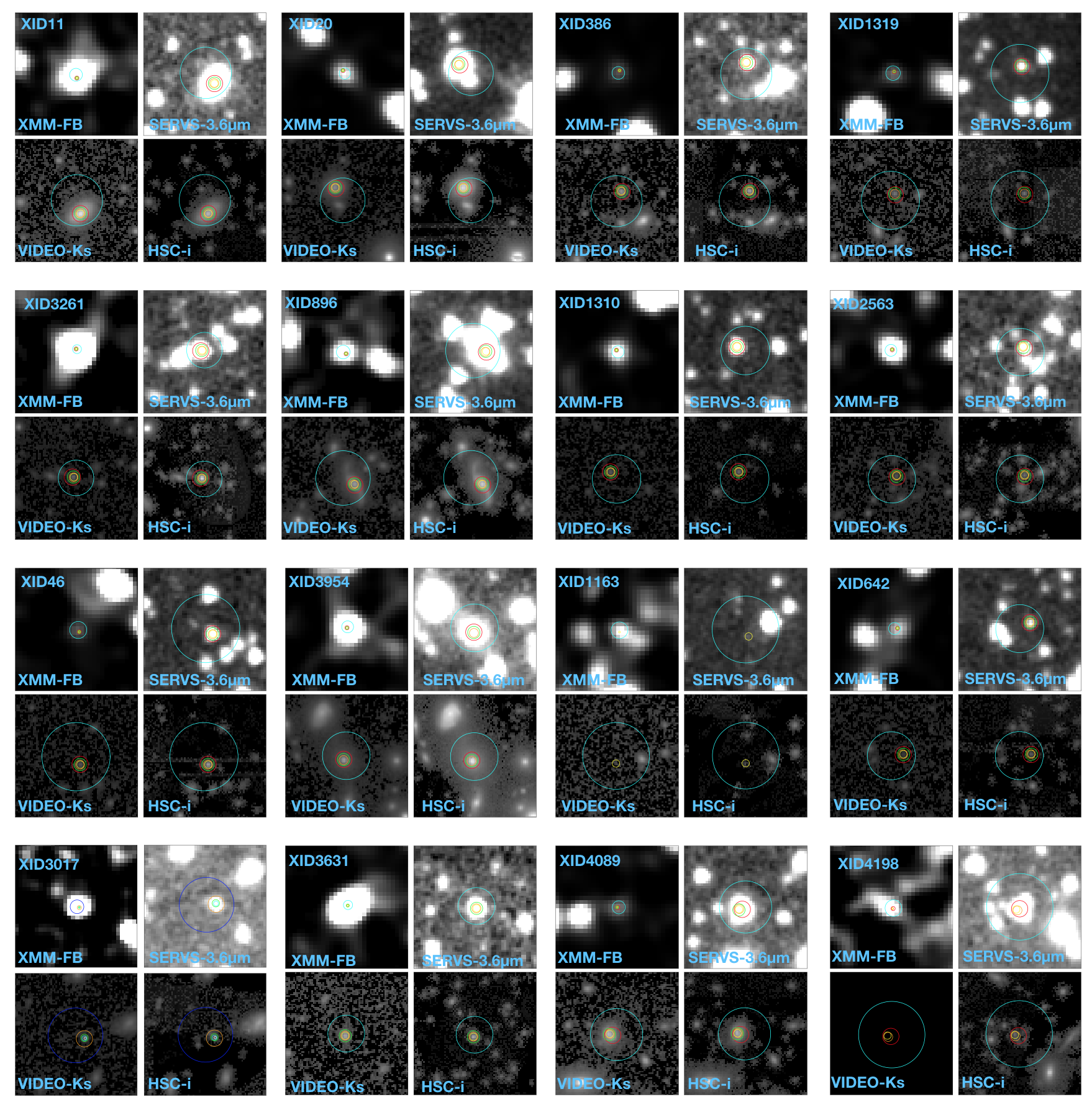
Figure 16: Postage-stamp images for 16 randomly selected X-ray sources in our catalog. For each source, we show (1) Full-band X-ray image smoothed with a Gaussian filter (upper-left panel). The unique source ID from Table A is shown in this panel. (2) 3.4$\mu$m mid-IR image from SERVS (upper-right panel) (3) Ks-band near-IR image from VIDEO (lower-left panel) (4) i-band optical image from HSC-SSP (lower-right panel), re-sampled to a 0$\aas@@fstack{\prime\prime}$4 pixel size. Due to the large pixel size, the X-ray image for each source is set at $2^{\prime}\times 2^{\prime}$. For the OIR images, the sizes are set at $0.5^{\prime}\times 0.5^{\prime}$. In each image, the X-ray position is marked as the cyan circle with the $r_{99}$ radius. The position of the most-probable mid-IR SERVS counterpart is marked as the red circle with a 1$\aas@@fstack{\prime\prime}$5 radius. The positions of VIDEO, CFHTLS, and HSC-SSP counterparts are marked as green, orange, and yellow circles with a 0$\aas@@fstack{\prime\prime}$9, 0$\aas@@fstack{\prime\prime}$6, and 0$\aas@@fstack{\prime\prime}$3 radius, respectively. The size of the OIR counterpart circles are 3 times the positional uncertainty values reported in Table 4. The entire set of postage-stamp images is available in the electronic version.

For the 4335 X-ray sources with primary counterparts from SERVS or VIDEO (regardless of matching reliabilities), 269 of them have no optical counterparts in CFHTLS and HSC-SSP. Visual inspection suggests that most of these sources are genuinely optically-faint. For 33 of the 269 sources, the optical counterpart is a bright star (or in the vicinity of one), and the photometry is unavailable from the CFHTLS or HSC-SSP catalogs due to saturation. There are also 1217 X-ray sources without a VIDEO counterpart, of which 787 are not in the footprint of VIDEO. For the remaining 430 X-ray sources without VIDEO photometry, visual inspection suggests that most of them are indeed NIR-faint, except for these 42 sources that either coincide with a bright star or are located on artifacts such as satellite tracks. To obtain useful OIR information for sources without reliable optical or NIR photometry, we search for counterparts in several additional OIR surveys with footprint in our X-ray catalog region, including the Sloan Digital Sky Survey (York et al., 2000) Data Release 12 (SDSS, Alam et al., 2015), the Two Micron All Sky Survey (2MASS, Skrutskie et al., 2006), and the UK Infrared Telescope Deep Sky Survey (the Deep Extragalactic Survey layer, UKIDSS-DXS; Warren et al. 2007). For our X-ray sources catalog, we only search for counterparts in these catalogs that are within 1^′′ of the OIR positions of the primary counterparts. With the supplementary catalogs, we recover the optical photometry for the 33 sources that do not have pipeline photometry from CFHTLS and HSC-SSP. We also identify an additional 333 sources with NIR photometry from 2MASS or UKIDSS-DXS. The basic properties of counterparts in these supplementary catalogs are also reported in the final source catalog (Table F).

There are also $1034$ sources with multiple counterparts having $LR>LR_{\rm th}$ and $LR>0.5LR_{\rm primary}$ in various OIR catalogs. For these sources, we select a “secondary” counterpart based on the following priority order: (i) 235 best matches from VIDEO; (ii) 48 second-best matches from SERVS; (iii) 79 second-best matches from VIDEO; (iv) 290 best matches from CFHTLS; (v) 223 best matches from HSC; (vi) 79 second-best matches from CFHTLS; and (vii) 80 second-best matches from HSC. Finally, there are 25 X-ray sources with three reliable counterparts; these tertiary counterparts are from VIDEO (4), CFHTLS (5) and HSC (16).

For the 1034 X-ray sources with secondary and/or tertiary counterparts, 869 of them have a SERVS source as the primary counterpart. Due to the larger PSF size of Spitzer IRAC ($\approx 2^{\prime\prime}$ at [3.6$\mu m$]) compared to the other OIR catalogs used in this work, it is possible that some of these secondary/tertiary counterparts from VIDEO, CFHTLS, or HSC-SSP are blended with the primary counterparts in the Spitzer image. Among these 1034 X-ray sources, a total of 318 of them are matched to a primary SERVS counterpart which appears to be two sources separated by $<2^{\prime\prime}$ in higher angular resolution bands. These counterparts are flagged in our final catalog. Excluding these 318 X-ray sources with potentially blended SERVS counterparts, the vast majority ($\approx 85\%$) of X-ray sources with secondary and/or tertiary counterparts have a primary counterpart with $MR>0.9$, suggesting that these additional counterparts are unlikely to be true counterparts of the X-ray sources. For completeness, these secondary and tertiary counterparts are also reported in our final catalog in Table F.

4.2 Counterpart identification reliability

We assess the reliability of the $LR$ matching results using the Monte Carlo simulation approach described in Broos et al. (2007) and Xue et al. (2011). Compared to the simple estimation based on matching OIR catalogs to a random X-ray catalog, the Broos et al. (2007) method usually provides a more realistic assessment of the matching reliability. As described in Broos et al. (2007) and Broos et al. (2011), we consider our X-ray sources to consist of two different intrinsic populations, the “associated population” and the “isolated population”. The associated population is comprised of X-ray sources that do have a real counterpart in the corresponding OIR catalog, and the X-ray sources that should not have any OIR counterparts belong to the isolated population.

For the associated population, counterpart-matching procedures can produce three different outcomes: (1) an X-ray source is matched to its correct counterpart (correct match, or CM), (2) an X-ray source is matched to an incorrect counterpart (incorrect match, or IM), and (3) no counterparts were recovered (false negative, or FN). The spurious fraction of the associated population is defined as $N_{\rm IM}/(N_{\rm IM}+N_{\rm CM})$. For the isolated population, there are two possible matching results: (1) no counterparts are found (true negative, or TN), and (2) an OIR source is identified as a counterpart (false positive, or FP). The spurious fraction of the isolated population is defined as the number of FPs divided by the size of the X-ray catalog. By definition, the spurious matches for these two populations are intrinsically different. The chance for the X-ray sources in the isolated population to have a counterpart is mostly determined by the source surface density of the OIR catalog being matched. On the other hand, since X-ray sources in the associated population must have a real OIR counterpart within a reasonable search radius, the spurious fraction is essentially determined by how well the $LR$ matching method can discern a real counterpart from background sources.

In order to estimate the fractions of X-ray sources in both populations for our catalog, we simulate each population separately. The details of the simulation procedure can be found in the appendix of Broos et al. (2007) and §5 of Broos et al. (2011). A brief summary of the simulations is given below: (1) For the “associated population”, we remove all OIR sources considered to be a match in §4.1, then move the position of each OIR source by 1^′ in a random direction. We then generate fake OIR “counterparts” for each X-ray source in our catalog based on the X-ray and OIR positional uncertainties, and the expected magnitude distributions derived in §4.1. (2) For the “isolated population”, we create mock X-ray sources that are at least 20″ away from any real X-ray sources.

A total of 100 simulations are carried out for each population, and we run the $LR$ matching procedures on each simulation as described in §4.1. The simulations of the isolated populations usually produce a much higher spurious fraction (i.e., the number of false-positives divided by the size of the X-ray catalog). For the SERVS, VIDEO, CFHTLS, and HSC-SSP catalogs, the median spurious fractions of the isolated populations are 19%, 24%, 30%, and 40%, respectively. For the associated populations, the spurious fractions (defined as $N_{\rm IM}/(N_{\rm IM}+N_{\rm CM}$)) for SERVS, VIDEO, CFHTLS, and HSC-SSP are 3%, 5%, 7%, and 9%, respectively.

For the $LR$ matching results with the real data, X-ray sources that were not reliably matched to any counterparts (with a total number of $N_{\rm negative}$) should contain a mixture of the FNs of the associated population and the TNs of the isolated population. Therefore, we can use the median FN and TN from simulations to estimate the fraction of X-ray sources in the associated population ($f_{\rm AP}$):

$$N_{\rm negative}=N_{\rm FN}\times f_{\rm AP}+N_{\rm TN}\times(1-f_{\rm AP}).$$ (9)

With $f_{\rm AP}$, we can estimate the expected number of X-ray sources that have a spurious match as the weighted sum of the numbers of IM and FP. The false-matching rate, $f_{\rm False}$, should therefore be:

$$f_{\rm False}=(N_{\rm IM}\times f_{\rm AP}+N_{\rm FP}\times(1-f_{\rm AP}))/(N_{\rm positive}).$$ (10)

Here we consider $N_{\rm positive}$ as the combination of both the “reliable” and “acceptable” matches reported in Table 4.

We carry out simulations for each OIR catalog. The values of $f_{\rm False}$ and $f_{\rm AP}$ for each OIR catalog are also reported in Table 4. Due to the high $f_{\rm AP}$ values, the false-matching rates of our matching results are mostly determined by the spurious fractions of the associated populations, which are much lower than those of the isolated populations. Adopting the Chandra-matched counterpart magnitude density, $q(m)_{\it Chandra}$, does reduce the false-matching rates compared to those derived using $q(m)_{\it XMM-Newton}$. For the SERVS and VIDEO catalogs, the improvements are marginal ($<0.5\%$), while the improvements for CFHTLS and HSC-SSP are more significant ($\approx 2\%$ and $6\%$, respectively).

We further scrutinize the $LR$ matching reliabilities by making use of the 223 CSC sources and their multiwavelength matching results described in §4.1. We assess the reliability of the matching results of these Chandra sources using the Monte Carlo method above, and measure false-match fractions of 0.9%, 1.4%, 2.8%, and 3.3%, for SERVS, VIDEO, CFHTLS, and HSC-SSP, respectively. For each catalog, we also directly compare the reliable matches obtained with XMM-Newton and Chandra positions; 97%, 94%, 91%, and 87% of the reliable Chandra matching results and the reliable XMM-Newton results are the same for the SERVS, VIDEO, CFHTLS, and HSC catalogs, respectively. The high “identical fractions” between the matching results obtained using Chandra positions and XMM-Newton positions are slightly lower than the false-matching rates calculated based on the Monte Carlo simulation because we only compare X-ray sources with reliable counterparts at the Chandra and XMM-Newton positions in each catalog. Similar to what was done for the full XMM-Newton catalog, we also select “primary” counterparts for the Chandra sources using the same priority orders. 85%, 10%, 1%, and 4% of the Chandra sources have their “primary” counterparts from SERVS, VIDEO, CFHTLS, and HSC-SSP, respectively. When comparing the primary counterparts of these Chandra sources and the primary counterparts of the corresponding XMM-Newton sources, $\approx 97\%$ are identical, demonstrating that the matching results of the XMM-Newton catalog are highly reliable.

4.3 Supplementary multiwavelength matching results with the NWAY Bayesian catalog matching method

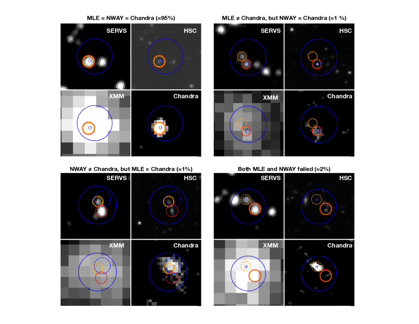
Figure 17: Illustrations of the comparison between the matching results using XMM-Newton positions or Chandra positions for four X-ray sources in our sample. The panel for each source shows images from SERVS [3.6$\mu$m](top-left), HSC i-band (top-right), XMM-Newton 0.5–10 keV (bottom-left), and Chandra 0.5–7 keV (bottom-right). X-ray positions are marked as blue circles with a 99.73% error radius, with the XMM-Newton positions indicated using solid lines and the Chandra positions identified using dashed lines. SERVS counterparts identified with the $LR$ method are marked as orange circles with a $2^{\prime\prime}$ radius, solid lines are the counterparts of the XMM-Newton positions, and dashed lines are the counterparts of the Chandra positions. SERVS counterparts of the XMM-Newton positions identified using NWAY are shown as the red circles. For the vast majority of XMM-Newton sources with Chandra counterparts from CSC, our counterpart-matching results are identical to the results obtained using Chandra coordinates and positional uncertainties.

We supplement the $LR$ matching results with the Bayesian catalog matching tool NWAY (Salvato et al., 2017). The fundamental difference between the Bayesian approach and the likelihood-ratio approach is that the former makes use of the distance and magnitude priors from multiple catalogs simultaneously to select the most-probable counterpart in all catalogs considered. NWAY also allows cases in which counterparts can be absent, and the matching results were computed considering all possible combinations. The details of the NWAY matching methodology are described in Appendix B of Salvato et al. (2017).

NWAY computes three quantities for deciding the most-probable match, $p\_single$, $p\_any$ and $p\_i$, where each possible counterpart has a different $p\_single$ value based on its distance from the XMM-Newton position. This value could be weighted by the priors supplied (e.g., $q(m)$ and $n(m)$ in Eq. 6 are similar to a magnitude prior). In our case, $p\_single$ is the posterior probability for a counterpart to be correctly associated with the X-ray source based on the angular separation from the X-ray position weighted by the magnitude-distribution prior, and the surface densities of the X-ray and OIR catalogs. For each X-ray source, $p\_single$ of all possible counterparts is considered to compute a single $p\_any$ value, which represents the posterior probability of the X-ray source having any correct counterparts (i.e., $p\_any=0$ if there are no OIR counterparts within the search radius of the X-ray source). The last quantity, $p\_i$, is the relative probability of a possible counterpart being the correct match. For an X-ray source with multiple possible counterparts, the counterpart with the highest $p\_i$ ($p\_i_{\rm Best}$) is considered to be the most-probable match and is assigned the match_flag = 1 flag by NWAY. Counterparts with $p\_i$ higher than 50% of $p\_i_{\rm Best}$ are also flagged by NWAY as match_flag = 2.

Similar to our $LR$ approach, we make use of the Chandra sources in the XMM-LSS field to compute the priors of the expected counterparts. We use the “auto” functionality of NWAY with a 1.5^′′ search radius for defining the “real” counterparts. In addition to the magnitude priors, we include an additional prior based on the Spitzer IRAC color from SERVS, [$3.6\mu$m]/[$4.5\mu$m]. Since the majority of our X-ray sources are expected to be AGNs, the distinct [$3.6\mu$m]/[$4.5\mu$m] mid-IR color of luminous AGNs (see Fig. 24) provides additional discerning power. For a small number of sources, this additional prior is useful for discerning two adjacent SERVS sources with comparable magnitudes (see the top-right panel of Fig. 17 for illustration).

After computing the magnitude and IRAC color priors using the Chandra sources, we run NWAY on the full X-ray catalog with a search radius of 10^′′. Based on the results from $LR$ matching (§4.1), we do not assume a completeness prior because only 0.01% of the X-ray sources are completely isolated. All four OIR catalogs are considered simultaneously. We report the multiwavelength matches with match_flag$=$1,2 in Table G supplementary to the $LR$ matching results.

Since NWAY matches all four OIR catalogs simultaneously, we cannot determine the spurious-matching rates for the “associated” and “isolated” populations as we did for estimating the spurious-matching rates for $LR$ results using Monte Carlo simulations (see §4.2). Salvato et al. (2017) suggest that the NWAY matching reliability can be determined by a $p\_any$ threshold, which is chosen based on re-running NWAY on randomly shifted “fake” X-ray catalogs. However, this approach is equivalent to estimating the spurious matching rates for the “isolated” population using the Broos et al. (2007) method, which is usually much higher than the results obtained with the two-population approach (see Broos et al. 2007, Xue et al. 2011, and §4.2 for details). Therefore, we do not adopt any $p\_any$ thresholds for the NWAY matching results. The NWAY matching results can still be assessed by investigating the CSC-matched subsample of 223 X-ray sources; the difference between the matching results obtained using Chandra and XMM-Newton positions with NWAY are similar to the $LR$ results described in §4.2.

We also use the 223 Chandra-detected subsample as a baseline for comparing matching results obtained using the NWAY or $LR$ methods. We focus only on comparing the SERVS counterparts, as the vast majority of $LR$ matching results are decided based on the primary counterparts from SERVS. We confirm that all Chandra sources have the same SERVS matching results using $LR$ and NWAY. Therefore, we can use the Chandra results obtained with $LR$ to assess the matching reliability of both $LR$ and NWAY matching results with XMM-Newton positions. Examples of such comparisons are shown in Fig. 17. $96\%$ of the sources have the same matching results from LR, NWAY, and Chandra. A small fraction (two sources) of $LR$ matching results do not agree with those of Chandra but could be recovered by NWAY. On the other hand, two of the NWAY matching results do not agree with the Chandra results but could be identified by LR. Five of the Chandra sources have different SERVS counterparts than both the $LR$ and NWAY results. Chandra and OIR images of these sources suggest that they are either two X-ray sources blended due to the XMM-Newton PSF, or there are multiple OIR counterparts with very similar magnitudes and distances to the X-ray position, and thus it is not surprising neither $LR$ nor NWAY could successfully recover the correct counterparts. As demonstrated in Fig. 17 (bottom-left), these five sources have multiple counterparts with comparable magnitudes and similar spatial separations from the XMM-Newton position. This result suggests $LR$ and NWAY perform similarly for finding SERVS counterparts. For the two X-ray sources with different LR and NWAY counterparts, their X-ray fluxes are relatively low (with a median full-band flux of $7.5\times 10^{-15}$ erg cm^-2 s^-1, which is $\approx 44\%$ of the median flux of the full X-ray catalog). This is expected as fainter X-ray sources have larger positional uncertainties, which leads to higher numbers of counterpart candidates.

When further scrutinizing the $96\%$ of sources with identical SERVS counterparts from LR, NWAY, and Chandra, we find that NWAY occasionally (for $\sim 10\%$ of the X-ray sources) considers the best-fit combination to be the one with counterparts in some of the other OIR catalogs being “absent”. For instance, one of the X-ray sources has a reliable SERVS counterpart identified by both NWAY and $LR$. For the SERVS counterpart, there is only one VIDEO source within the 0.5^′′ positional error circle of SERVS. For the $LR$ approach described in §4.1, the VIDEO source is assigned to the correct SERVS counterpart. However, NWAY does not consider this VIDEO source to be among the most-probable combination of counterparts from all four OIR catalogs that were being matched simultaneously. This result is likely due to how NWAY computes $p\_i$. When multiple OIR catalogs are taken into account simultaneously, $p\_i$ represents the relative probability of counterparts from all OIR catalogs being the correct match. In this example, the VIDEO counterpart has an unlikely magnitude according to the VIDEO magnitude prior; therefore, including the VIDEO source as a correct match would result in a lower $p\_i$ compared to the case where the VIDEO source is excluded from the matched counterparts. Similar mismatches are found when comparing the NWAY and $LR$ matching results for the full XMM-Newton catalog. Note that the p_any values for these sources are generally lower (with a median of 0.16) compared to the sources without such problems (their median p_any$=0.98$), but sources with p_any$>0.98$ can still have this behavior. NWAY does not have this behavior when no magnitude or color priors are used; however, without the inclusion of magnitude and color priors, NWAY can only rely on the distance-based priors, thereby losing critical discerning powers for matching XMM-Newton sources to the dense OIR catalogs. Further corroborating the Bayesian method’s effectiveness of counterpart-matching with multiple OIR catalogs is beyond the scope of this work. Therefore, we list the NWAY matching results “as-is” in Table G, and we consider only the $LR$ matching results listed in Table F when exploring the multiwavelength properties of the X-ray sources reported in this work. The matching results obtained using NWAY are shown in Table G, and the descriptions of this table’s columns are listed in Appendix B. Only the counterparts with match_flag$\geq 1$ are included.

5 Redshifts

5.1 Spectroscopic redshifts

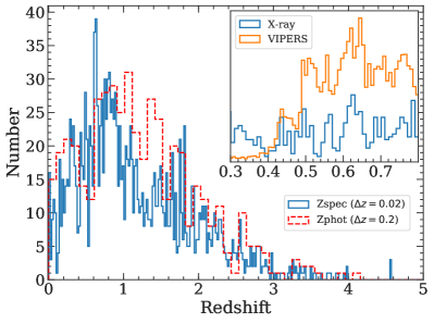
Figure 18: Distribution of the redshifts in bins of $\Delta z=0.02$ for the 1782 X-ray sources with spectroscopic-redshift measurements from the literature. The photometric-redshift distribution for the 2105 sources with high-quality photometric redshifts is also plotted as the red dashed histogram in bins of $\Delta z=0.2$. The redshift spikes are likely associated with large-scale structure filaments (e.g., Luo et al., 2017; Xue, 2017). A comparison between the normalized redshift distribution of the X-ray sources and that of the $i$-band selected galaxies from the VIPERS survey is also shown in the insert with $\Delta z=0.01$ bins, which suggests that some of the redshift spikes (e.g., $z\approx 0.6$) of X-ray sources overlap with those of the general galaxy population.

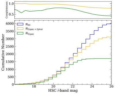
Figure 19: The blue histogram shows the cumulative distribution of the HSC i-band magnitudes for 4012 i-band-detected X-ray sources in the $4.5$ deg² subfield covered by the N18 forced-photometry catalog (see §5.2). The cumulative distribution of the sources with spectroscopic redshifts is indicated by the green histogram, and the cumulative distribution of the sources with high-quality photometric or spectroscopic redshifts is indicated by the orange histogram. The top panel shows the fraction of sources with spectroscopic redshifts (i.e., the green histogram divided by the blue histogram) as a function of i-band magnitude. The fraction of sources with good photometric or spectroscopic redshifts as a function of i-band magnitude is shown as the orange curve.

Table 5: Redshift catalogs used in this work. Column 1: Redshift survey name. Column 2: Survey instrument. Column 3: Survey sensitivity. Column 4: Targeting fields. Column 5: Survey area. Column 6: Total number of redshifts matched the main X-ray catalog. Column 7: Total number of redshifts assigned to the X-ray sources in the main catalog. Column 8: Reference

Catalog	Instrument	Survey sensitivity	Targeting fields	Area	$N_{\rm matched}$	$N_{\rm assigned}$	Reference
(1)	(2)	(3)	(4)	(5)	(6)	(7)	(8)
SDSS	BOSS	$r\lesssim 22.5$	XMM-XXL-North	25 deg2	1075	1075	Dawson et al. (2013);
							Menzel et al. (2016)
PRIMUS	IMACS	$i\lesssim 23.5$	XMM-LSS	2.9 deg2	749	347	Coil et al. (2011)
	(Low-Dispersion Prism)
VIPERS	VIMOS	$i\lesssim 22.5$	XMM-LSS	7.8 deg2	332	161	Garilli et al. (2014)
UDS Compilation	Multiple instruments	N/A	UDS	0.8 deg 2	302	72	N/A (see Footnote 25)
CSI	IMACS	[3.6$\mu$m]${}_{\rm AB}\lesssim 21$	XMM-LSS	6.9 deg2	516	68	Kelson et al. (2014);
	(Uniform-Dispersion Prism)						Patel et al. (2015)
VVDS	VIMOS	$17.5\lesssim i\lesssim 24.5$	XMDS+SXDS	3 deg2	81	38	Le Fevre et al. (2013)
UDSz	VIMOS/FORS2	$K<23$	UDS	0.5 deg2	22	15	Bradshaw et al. (2013);
							McLure et al. (2013)
3D-HST	WFCS G141 Grism	$JH_{\rm IR}\lesssim 24$	UDS	191.2 arcmin2	15	6	Skelton et al. (2014);
							Momcheva et al. (2016)

The XMM-LSS region is covered by a number of spectroscopic redshift (spec-z) surveys that target galaxies with various optical magnitude constraints: the PRIsm MUlti-Object Survey (PRIMUS; Coil et al., 2011), the VIMOS Public Extragalactic Redshift Survey (VIPERS; Garilli et al., 2014), and the VIMOS VLT Deep Survey (VVDS; Le Fevre et al., 2013). As part of the SDSS Baryon Oscillation Spectroscopic Survey (SDSS-BOSS) program, 3042 X-ray sources found in the XMM-XXL-North field (25 deg²) with $r<22.5$ were all observed by the SDSS-BOSS (Dawson et al., 2013; Menzel et al., 2016). Also, there are three other redshift surveys in the XMM-LSS region that target near-IR selected galaxies, including the spectroscopic observations of the UKIDSS Ultra-Deep Survey (UDSz; Bradshaw et al., 2013; McLure et al., 2013), the 3D-HST Survey (Skelton et al., 2014; Momcheva et al., 2016) in the UDS region, and the Carnegie-Spitzer-IMACS Redshift Survey (CSI; Kelson et al. 2014). We list the properties of each redshift catalog in Table 5.

We adopt the same nearest-neighbor matching criterion with a 1^′′ matching radius to associate these redshifts to each OIR catalog. The redshift for each X-ray source is determined by the coordinates of its primary OIR counterpart. In cases where redshifts from different catalogs do not agree with each other, we choose redshifts using the following ordering (ranked by the spectral resolution at r-band and reliability): SDSS, VVDS, VIPERS, UDSz, PRIMUS (reliable), CSI (reliable), 3D-HST, PRIMUS (acceptable), and CSI (acceptable). In addition to these redshift surveys, we include the compilation of $\approx 4000$ publicly available but unpublished redshifts in the UDS field. An additional 72 X-ray sources have spec-zs culled from this catalog. We also search for publicly available spec-zs for all of our counterparts not included in the aforementioned redshift catalogs in the NASA Extragalactic Database (NED), but no additional secure redshifts were found.

Of the 5242 sources in our main X-ray source catalog, 1782 have spec-zs ranging from $0<z<4.57$. Fig. 18 presents the redshift histogram in bins of $\Delta z=0.02$. There are several redshift “spikes” indicative of large-scale structures containing X-ray AGNs (e.g., Fig. 9 of Luo et al. 2017 and Fig. 20 of Xue 2017). Notably, the X-ray source redshift spike at $0.6<z<0.7$ appears to coincide with one of the major large-scale structures seen in the VIPERS redshift survey (see Fig. 14 of Garilli et al. 2014 and the insert panel of Fig. 18). The cumulative histogram of the i-band magnitudes of the sources with spec-zs is shown in Fig. 19 as the green histogram.

5.2 Photometric redshifts

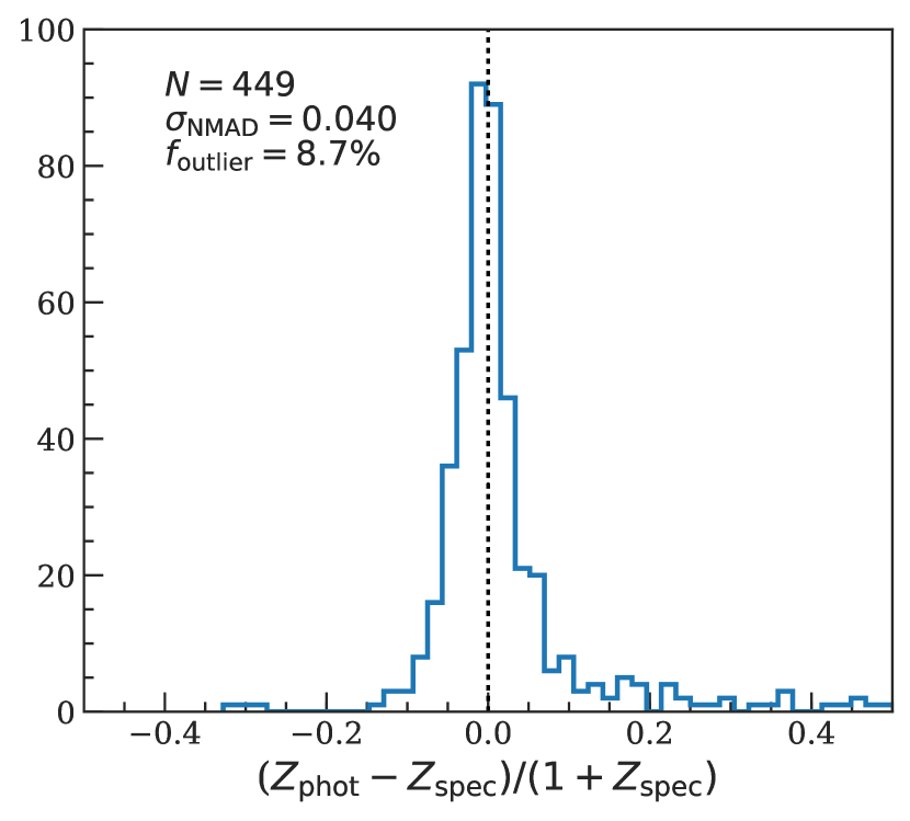
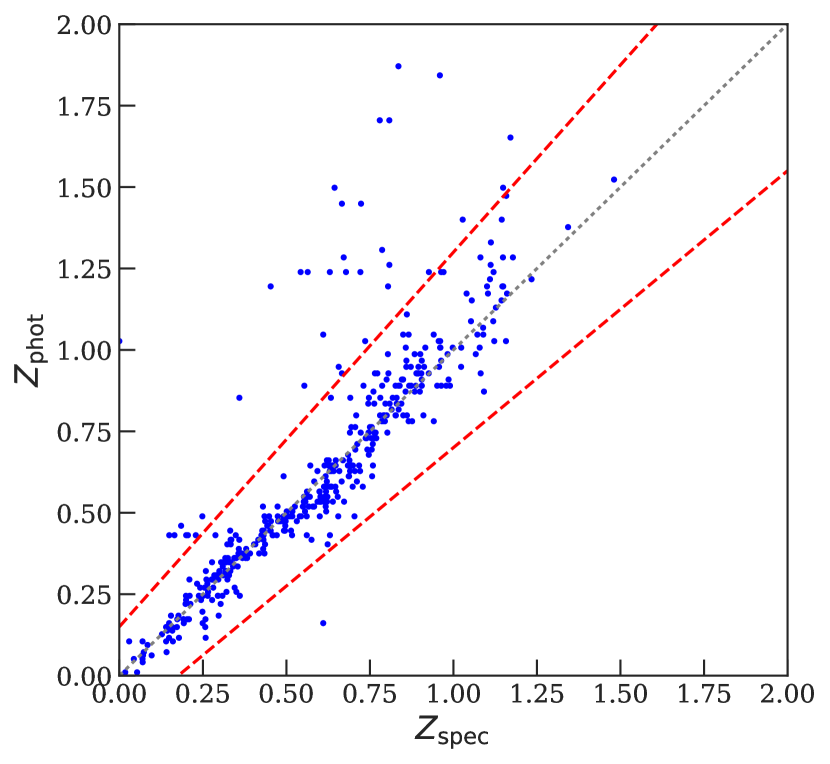
Figure 20: Spectroscopic and photometric redshifts for the 449 non-broad-line AGN sources with high-quality photo-zs and spec-zs. The left panel shows the histogram of the fractional difference between the photo-zs and the spec-zs. The right panel shows the direct comparison between the photo-zs and the spec-zs. The black dotted lines in both panels mark the $z_{\rm spec}=z_{\rm phot}$ relation. In the right panel, the red dashed lines mark the $\mathopen{|}\Delta z\mathclose{|}/(1+z_{\rm spec})=0.15$ thresholds for outliers.

High-quality photometric redshifts (photo-zs) for AGNs are not yet available for our full survey region, but they are available in a number of smaller subfields. In particular, in a $\approx 1$ deg² area within the XMM-LSS region, Nyland et al. (2017) have presented a “forced-photometry” catalog using the Tractor image-modeling code (Lang et al., 2016). The forced-photometry technique employs source-position and surface-brightness profile priors from the high-resolution fiducial band of the VIDEO survey to model and fit the fluxes of lower-resolution bands. Nyland et al. (2017) demonstrated that their multi-band forced photometry of mixed resolution optical and IR surveys using the Tractor led to a statistically significant improvement in photometric-redshift accuracy compared to position-matched multi-band catalogs (see §5.2 of Nyland et al. 2017 for details). For this work, we make use of a similar forced-photometry catalog for the full 4.5 deg² area with VIDEO and SERVS coverage (Nyland et al. 2018, in preparation; N18 hereafter). The N18 catalog is similar to the Nyland et al. (2017) catalog, except the image cutout width for each source has increased by a factor of two (from 10^′′ to 20^′′) and the sky noise and sky level are now calculated in each image cutout using iterative sigma clipping. Also, N18 used IRAC data from the SERVS DeepDrill survey (P.I. Mark Lacy), which expands upon the coverage of the SERVS project by providing deep IRAC imaging to microJy-depth of the four predefined Deep Drilling Fields for the LSST. In the XMM-LSS field, the DeepDrill data more than double the footprint of the SERVS post-cryogenic data, thus leading to higher-quality data along the edges of the SERVS coverage where there is overlap with the VIDEO data. Thus, our IRAC 3.6 and 4.5 $\mu$m photometry is based on the DeepDrill data. We make use of the 13-band photometry from u^′ to IRAC 4.5$\mu$m to derive photo-zs for the X-ray sources in this region using the methods described in Yang et al. (2014). The photometric bands include CFHTLS $u$-band; HSC-SSP g, r, i, z, and y bands (wide layer); VIDEO Z, Y, J, H, and Ks bands (DR5); and Spitzer 3.6 $\mu$m and 4.5 $\mu m$ bands from the SERVS DeepDrill survey.

We match the N18 catalog to the coordinates of the primary counterparts of the X-ray sources that are considered to be reliable matches using a 1^′′ matching radius. We exclude the 930 X-ray sources that are classified as broad-line AGNs (see §6 for details) according to their optical spectra due to their much higher photometric-redshift uncertainties. A total of 3418 X-ray sources satisfy these criteria. Of these sources, $\approx 38\%$ of them are detected (i.e., with Tractor measured signal-to-noise-ratio $>5$) in all 13 bands. The 25th, 50th, and 75th percentiles of the number of bands with detection for the 3418 X-ray sources are 10, 11, and 13. Since the flux uncertainties in N18 do not account for uncertainties in the PSF homogenization processes, we adopt an additional 3% systematic for the flux errors, which is typical of PSF modeling uncertainties (e.g., §5.3 of Yang et al. 2014).

Following the approach of Yang et al. (2014), we measure the photo-zs using the SED-fitting code eazy (Brammer et al., 2008) using the default galaxy templates and settings, and an additional obscured AGN template from Polletta et al. (2007). As described in §5.6 of Yang et al. (2014), we perform iterative procedures to adjust the photometric zero points; the zero-point corrections are $\lesssim 0.1$ mag. For each source, eazy calculates a parameter $Q_{z}$ (see Eq. 8 of Brammer et al. 2008) to indicate photometric-redshift quality. Of the 3418 non-broad-line X-ray sources with forced photometry, we consider the 2105 ($\approx 62\%$) photo-zs with $Q_{z}<1$ as reliable (see §6.3 of Yang et al. 2014). The fraction of sources with high-quality photo-zs becomes higher for brighter sources. For instance, sources with VIDEO $Ks$-band magnitude in the brightest 25th, 50th, and 75th percentiles (corresponding to $Ks<19.77$, 20.83, and 21.78) have $77\%,76\%$, and $71\%$ high-quality photoz-s, because fainter sources have larger photometric uncertainties and fewer photometric points. With the deep NIR coverage from VIDEO and SERVS, we can detect the Balmer break even for high redshift sources, hence the range of our $Q_{z}<1$ photo-zs extends to $z\approx 4$. There are 536 sources with $Q_{z}<1$ and reliable spec-zs. Of these sources, 449 of them have spectroscopic classifications from at least one of the public redshifts catalogs and are not classified as a broad-line AGN. Since we excluded broad-line sources, the spectroscopic redshift range of these sources is 0.02–1.5, with a median value of 0.79. We use these 449 sources to assess the quality of the 2105 photo-z measurements. The normalized median absolute deviation (NMAD) is $\sigma_{\rm NMAD}=0.040$, with an outlier fraction (defined as $\mathopen{|}\Delta z\mathclose{|}/(1+z_{\rm spec})>0.15$) of $f_{\rm outlier}=8.7\%$, which is comparable to the photometric-redshift reliability reported in Yang et al. (2014) for the CDF-N. A small fraction of sources are found to be outliers. This is likely caused by the photo-z code mistakenly identifying the location and strength of the prominent spectroscopic feature, the Balmer break (the lack of radiation at wavelength range $<3646$ Å ), due to photometric redshift uncertainties in one or more bands. We note that the majority of the outliers have $z_{\rm spec}<z_{\rm phot}$. This is expected for the $z_{\rm spec}\lesssim 1$ sources (e.g., see Fig. 14 of Yang et al. 2014), because only less than three photometric bands cover the rest-frame wavelength range of the Balmer break and it is difficult to identify a spectral break with only three photometric bands. Therefore, it is less likely for the aforementioned misidentifications to cause a $z_{\rm phot}$ lower than these low-spec-z sources. For this work, we do not include the broad-line AGN (BLAGN) templates as Yang et al. (2014) did. This is primarily driven by the worse photometric redshift qualities when including the BLAGN templates. In addition, Yang et al. (2018) estimated that the fraction of broad-line AGNs missed by spectroscopic campaigns in the COSMOS field is likely less than $\approx 18\%$. Considering the comparable surface density of the spectroscopically confirmed BLAGNs in this work and that in the COSMOS field, only a small fraction of sources would require an additional BLAGN template. In fact, the vast majority of our sources (excluding spectroscopically confirmed BLAGNs) can be well-characterized with galaxy templates alone, and the high fraction (see below) of our sources with high-quality photo-zs also justifies our choice of fitting templates.

Fig. 20 compares the photometric and spectroscopic redshifts for the 449 non-broad-line sources with reliable photo-zs. The 4.5 deg² area covered by N18 contains 1543 reliable photo-zs for sources that do not have spectroscopic redshift measurements, increasing the fraction of sources with redshifts from $\approx 32\%$ to $\approx 70\%$. We expect to expand the photometric-redshift measurements to all of our X-ray sources in the full XMM-SERVS:XMM-LSS field when the photometry catalog with data from both the SERVS DeepDrill survey (Spitzer Program ID 11086; Lacy et al., in preparation) and the VEILS survey (see Table 1) becomes available. We have also run our photometric-redshift codes on all sources in the preliminary N18 catalog, and we report the photo-zs for the 390,900 sources in Appendix C. The full details of the Tractor catalog over the 4.5 deg² field will be presented in Nyland et al. (2018, in preparation).

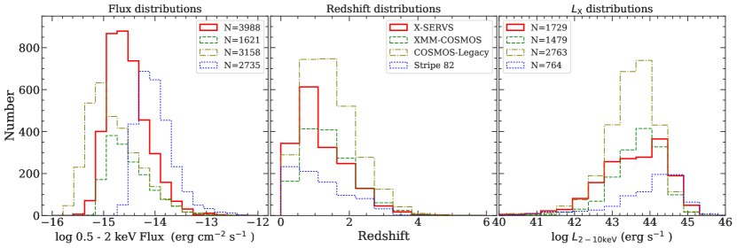
Figure 21: A comparison between this work (solid red line), XMM-COSMOS (green dashed line), COSMOS-Legacy (brown dash-dotted line), and Stripe 82–X (blue dotted line). Distributions shown in panels from left to right are: 0.5–2 keV flux, redshift, and $\log L_{\rm 2-10~{}keV}$, respectively. The left panel shows the distribution of soft-band fluxes for the soft-band detected sources in each catalog; no redshift information is required. The numbers of the soft-band sources are listed in the left panel. For the middle and right panels, the histograms are for the subset of sources with redshift measurements (regardless of the detection bands), with source numbers marked in the right panel.

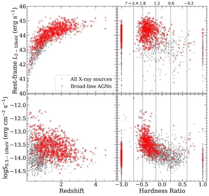
Figure 22: Properties of the 1782 X-ray sources with spectroscopic-redshift measurements, including the (1) $L_{\rm 2-10~{}keV}$ vs. $z$ distribution (top-left), (2) $L_{\rm 2-10~{}keV}$ vs. hardness ratio (top-right), (3) 0.5–10 keV flux vs. redshift (bottom-left), (4) 0.5–10 keV flux vs. hardness ratio (bottom-right). Broad-line AGNs are marked as the red open circles. In the right panels, the expected hardness ratios for power-law spectra (with Galactic column density) with different photon indices are plotted as the vertical dashed lines. Sources detected only in the soft or hard bands have their HR set at $-1$ and 1, respectively.

6 Source properties and classification

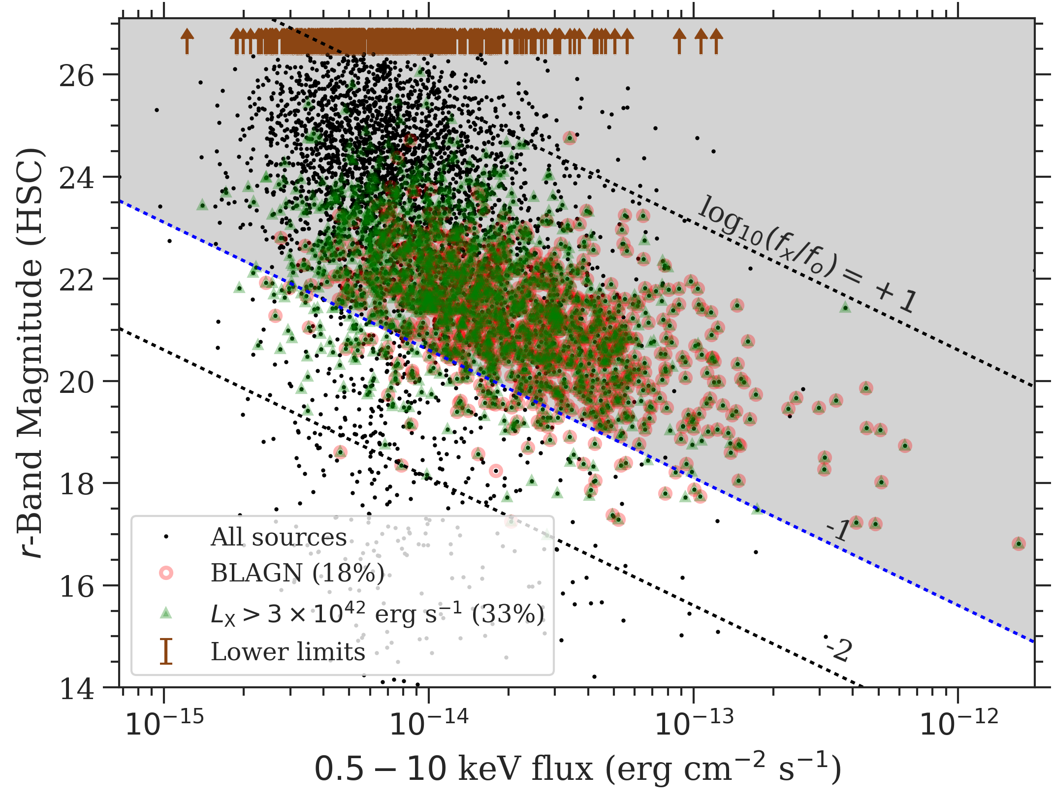
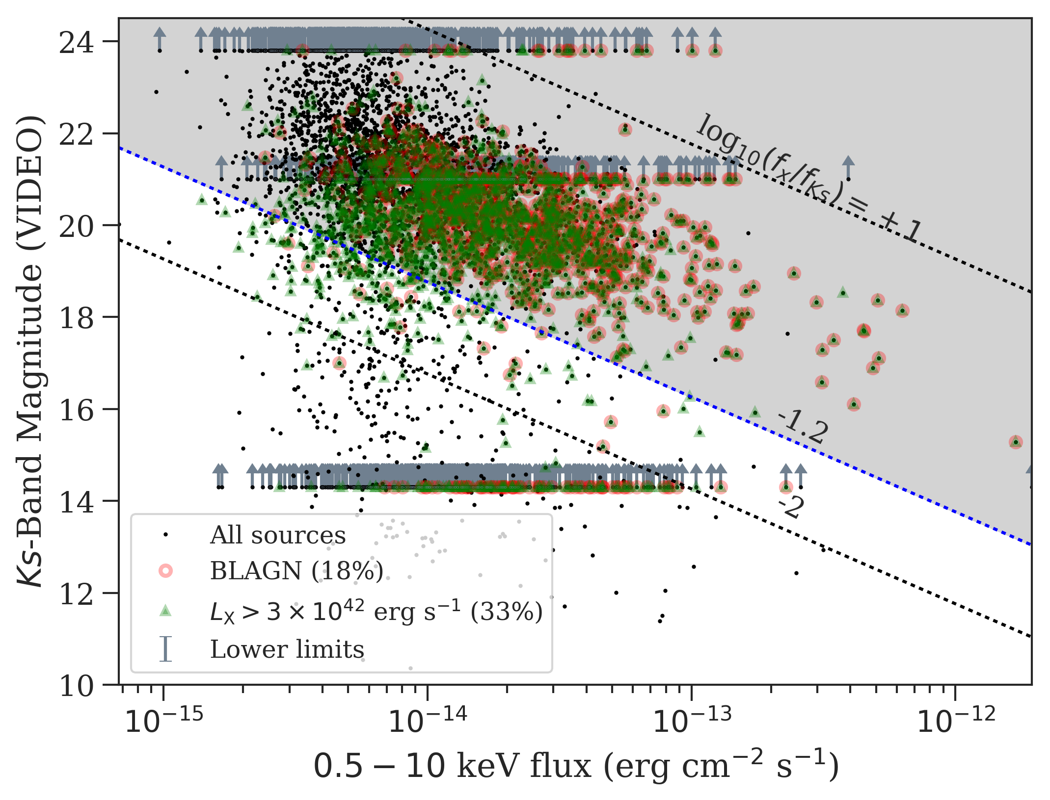
Figure 23: Left – Distributions of the optical flux in the r-band vs. full-band (0.5–10 keV) X-ray flux. Lower limits for sources not detected in the HSC-SSP wide survey r-band are displayed as the brown upward arrows. Right – The near-IR flux in the Ks-band versus full-band X-ray flux. Lower limits for sources not detected in VIDEO are also show as the upward arrows. Since only $\approx 85\%$ of the X-ray catalog region is covered with VIDEO, some of the X-ray sources have lower limits from 2MASS ($Ks=14.3$), UKIDSS DXS survey ($Ks=21$), and VIDEO ($Ks=23.8$). In both plots, the shaded regions mark the “AGN” regime as defined by the $\log_{10}f_{x}/f_{o}>-1$ (left) or the $\log_{10}f_{x}/f_{\rm Ks}>-1.2$ (right) thresholds as described in §4.5 of Luo et al. (2017). For sources with spectroscopic redshift measurements, we also mark those with $L_{\rm X}>3\times 10^{42}$ erg s^-1 as the green triangles. The 930 sources with optical spectra consistent with broad-line AGNs are also marked as open red circles.

In this section we briefly discuss some of the properties of the 4858 sources with reliable counterparts. For the 1782 X-ray sources with secure spec-zs, we calculate their rest-frame 2–10 keV “apparent” luminosity assuming a $\Gamma=1.7$ power-law spectrum corrected for Galactic absorption. Fig. 21 compares the flux, redshift, and luminosity distributions of our sample to those from archival X-ray surveys, including XMM-COSMOS, COSMOS-Legacy, and Stripe 82X. Fig. 22 displays the $L_{\rm X}-z$ distribution of our sample, along with the $L_{\rm X}$ vs. HR, HR vs. full-band flux, and full-band flux vs. redshift distributions. The comparisons in the middle and right panels of Fig. 21 are limited to sources with available spec-zs in the Stripe-82 and XMM-LSS regions. The left panel of Fig. 21 demonstrates that our catalog occupies a valuable region of parameter space among X-ray surveys by more than doubling the source counts of the XMM-COSMOS survey, which will enable a wide range of science that was previously limited by either survey sensitivity or cosmic variance.

For this work, we also include the basic AGN identification results in our catalog. Detailed source classifications using multiwavelength SED and X-ray spectroscopic fitting results will be saved for future works. For sources with spectroscopic observations, we directly make use of the spectroscopic classifications when available. Since each spectroscopic survey has its own unique design and methodology, we only make use of the “broad-line” classifications provided in the SDSS, VIPERS, VVDS, and PRIMUS catalogs to identify broad-line AGNs. The information on spectroscopic classifications is not yet publicly available for the other spectroscopic surveys. For each X-ray source with optical spectroscopic coverage, we have included the spectroscopic flags from all available redshift catalogs (see Column 184 of the main X-ray catalog described in Appendix A). A total of 930 sources are classified as AGNs based on the broad-line spectroscopic flags specified in the SDSS, VIPERS, VVDS, or PRIMUS catalogs. Since 90% of the spec-zs for our X-ray sources are culled from one of these four catalogs, we expect the vast majority of the remaining X-ray sources with spectroscopic coverage to have galaxy-like spectra. For sources without spectroscopic observations, only a small fraction of them is expected to be broad-line AGNs (see §5.2 and Yang et al. 2018 for details). For the other sources, we use the criteria described in Luo et al. (2017) to select AGNs: (1) An X-ray luminosity threshold where we regard sources with rest-frame $L_{\rm 2-10~{}keV}>3\times 10^{42}$ erg s^-1 as an AGN. A total of 1625 sources satisfy this criterion. (2) X-ray bright sources with X-ray-to-optical or X-ray-to-near-IR flux ratios larger than $\log f_{x}/f_{r}>-1$ or $\log f_{x}/f_{Ks}>-1.2$, respectively. To calculate the flux ratios, we use the HSC-SSP r-band photometry of the primary counterpart. For sources without a detection in the HSC-SSP r-band, we make use of CFHTLS or SDSS r-band photometry when available. For the 265 sources that are not detected in HSC-SSP, CFHTLS, or SDSS, we calculate their flux-ratio lower limits using the HSC-SSP wide survey upper limit, $r=26.4$. For the X-ray-to-near-IR flux ratios, we use the VIDEO Ks-band photometry. For sources within the VIDEO coverage but not detected in the Ks-band, we calculate the lower limits for $\log f_{x}/f_{Ks}$ assuming a $Ks=23.8$ upper limit. For sources outside the VIDEO coverage, we make use of the UKIDSS DXS survey Ks-band photometry when possible and assign an upper limit of $Ks=21$ for the non-detected sources. For sources outside the coverage of VIDEO and UKIDSS, the shallow photometric depth of 2MASS ($Ks<14.3$) cannot be used to select AGNs, since no sources this bright would have a high $\log f_{x}/f_{Ks}$ ratio satisfying the AGN selection criterion. There are 4998 sources with $\log f_{x}/f_{r}>-1$ and 4700 sources with $\log f_{x}/f_{Ks}>-1.2$, totaling 5064 sources that can be classified as an AGN based on their $f_{x}/f_{r}$ or $f_{x}/f_{Ks}$ values. The flux-ratio distributions are displayed in Fig. 23.

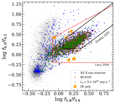
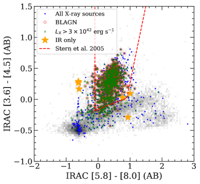
Figure 24: Left – $\log f_{5.8}/f_{3.6}$ vs, $\log f_{8.0}/f_{4.5}$ distribution. Right – IRAC$[5.8]-[8.0]$ vs. $[3.6]-[4.5]$ (AB) distributions. In both panels, the Spitzer IRAC two-color distribution for the 1716 X-ray sources with detections in all four IRAC bands are shown as the blue dots. X-ray luminous AGNs and spectroscopically confirmed quasars are also shown as the green triangles and the open red circles, respectively. There are a total of 1325 sources with IRAC colors satisfying one of the three mid-IR color AGN selection criteria (Lacy et al. 2004, Stern et al. 2005, and Donley et al. 2012). The six sources that are only identified as an AGN based on their IRAC colors are displayed as the large orange stars. The color distribution for the 12990 SWIRE sources in our X-ray catalog region is also shown as the gray hexagonal cells, where darker color indicates higher source density.

In addition to the classification methods described above, AGNs can also be identified based on the distinctive red mid-IR color arising from hot dust heated by SMBH accretion (e.g., Lacy et al., 2004; Stern et al., 2005; Stern et al., 2012; Donley et al., 2012; Assef et al., 2013; Mateos et al., 2013). We select these mid-IR AGNs based on three different selection criteria from Lacy et al. (2004), Stern et al. (2005), and Donley et al. (2012). The Lacy et al. (2004) and Stern et al. (2005) criteria have higher completeness while the Donley et al. (2012) criterion is more reliable (i.e., has much less star-forming galaxy interlopers). Only 1716 X-ray sources have a primary counterpart that is detected in all four IRAC bands, which is a requirement of using these IRAC two-color selection criteria. Of these 1716 sources, 1300, 1158, and 834 satisfy the Lacy et al. (2004), Stern et al. (2005), and Donley et al. (2012) criteria, respectively, for a total of 1325 individual X-ray sources. Notably, six sources are only identified as an AGN based on their IRAC colors. On the other hand, of all X-ray sources with detections in all four IRAC bands, 257 AGNs identified using the X-ray AGN selection criteria described in the previous paragraph do not satisfy any of the three IRAC color-color selection criteria. The IRAC color distributions of the 1716 X-ray sources, and the 12990 SWIRE sources in our X-ray catalog region are displayed in Fig 24.

The total number of sources classified as AGNs is 5071, or $96.7\%$ of the total sample. For the sources not classified as AGNs, 54 of them have spectroscopic-redshift measurements, including 13 stars with $z\approx 0$, and 41 galaxies hosting low X-ray luminosity sources. They may be powered by star-formation processes in galaxies given their relatively weak X-ray to OIR ratios and low X-ray luminosities. The remaining 117 sources are relatively bright in the optical and NIR bands (median r-band and Ks-band magnitudes are 15.5 and 14.1, respectively), and thus all of them have optical-to-X-ray and NIR-to-X-ray flux ratios lower than the AGN selection thresholds, suggesting they are either foreground stars or low-redshift galaxies hosting X-ray sources powered by stellar processes.

7 Summary

In this work, we present a new X-ray point-source catalog in the XMM-LSS region constructed using both considerable new AO-15 and archival XMM-Newton data. The main results are the following:

1. Our X-ray catalog is constructed based on data in a $5.3$ deg² rectangular region centered at RA$=35.580^{\circ}$, DEC=$-4.965^{\circ}$. A total of 155 pointings from 149 different XMM-Newton ObsIDs are used, with a total of $2.7$ Ms background-filtered exposure time (1.1 Ms from AO-15). The median value of the cleaned PN exposure time is 46 ks for the full 5.3 deg² field (see §2). Our survey has a flux limit of $1.7\times 10^{-15}$, $1.3\times 10^{-14}$, and $6.5\times 10^{-15}$ erg cm^-2 s^-1 over 90% of its 5.3 deg² area in the soft, hard, and full bands, respectively, reaching the desired uniformity and survey depth (see §3.6).

2. We use Monte Carlo simulations to estimate the fraction of spurious sources ($f_{\rm spurious}$) as a function of det_ml values for each band, and we consider sources with $f_{\rm spurious}\leq 1\%$ to be reliably detected. This corresponds to det_ml thresholds of 4.8, 7.8, and 6.2 in the soft, hard, and full bands, respectively (§3.3).

3. The main X-ray source catalog is generated using ewavelet and emldetect. All 5242 sources with emldetect det_ml values satisfying the $f_{\rm spurious}\leq 1\%$ criterion in the soft band (0.5–2 keV), hard band (2–10 keV), or full band (0.5–10 keV) are included. Of the 5242 sources, 2861 are the same X-ray sources identified in previous X-ray surveys in our survey area (e.g., the XMM-XXL-North survey; Liu et al., 2016), and 2381 are newly discovered X-ray sources (see §3.5). There are 2967 sources with more than 100 X-ray counts in the full band (PN + MOS), and 126 sources with more than 1000 X-ray counts (see §3.5).

4. The absolute astrometry of the XMM-Newton catalog is registered to the WCS frame of the Subaru HSC-SSP survey (§3.1). The positional uncertainties for the X-ray sources are determined based on an empirical relation between the X-ray-to-optical positional offsets and the X-ray source counts. Our empirical positional uncertainties are well-characterized by the Rayleigh distribution. The median positional uncertainties in the soft, hard, and full bands are 1$\aas@@fstack{\prime\prime}$35, 1$\aas@@fstack{\prime\prime}$37, and 1$\aas@@fstack{\prime\prime}$31, respectively (see §3.4).

5. We search for OIR counterparts in the SERVS, VIDEO, CFHTLS, and HSC-SSP surveys; $98\%$ (5147/5242) of the X-ray sources have at least one OIR counterpart candidate within the $99.73\%$ positional uncertainties ($r_{99\%}$). A total of $\approx 93\%$ (4858/5242) of the X-ray sources have at least one reliable OIR counterpart (§4.1). There are 1782 secure spectroscopic redshifts from SDSS, VIPERS, VVDS, UDSz, PRIMUS, CSI, and 3D-HST (§5.1). For a 4.5 deg² subfield in our survey region covered by SERVS, we make use of the forced-photometry catalog from N18 to compute photometric redshifts (§5.2), achieving $>70\%$ spectroscopic+photometric redshift completeness for $85\%$ of our survey area. We expect to expand the photometric redshift measurements to all of our X-ray sources when SERVS DeepDrill survey (Spitzer Program ID 11086; Lacy et al., in preparation) and the VEILS survey (see Table 1) are completed.

6. We test the matching results using a subsample of 223 X-ray sources with a reliable Chandra counterpart from CSC 2.0. Approximately $97\%$ of the matching results from XMM-Newton and Chandra are identical, demonstrating our multiwavelength matching results are highly reliable (see §4.2).

7. We classify 5071 X-ray sources as AGNs based on their optical spectra from SDSS, VIPERS, or VVDS (930); X-ray luminosity larger than $3\times 10^{42}$ erg s^-1 (1625); large X-ray-to-optical and/or X-ray-to-NIR flux ratios (5064); and Spitzer IRAC colors (1325). See §6 for details.

The X-ray source catalog presented in this work is the first $>2$ deg² X-ray survey with sensitivity comparable to that of COSMOS. This 5.3 deg² wide-area and 46 ks depth survey will enable a wide range of studies. For instance, the large AGN sample and the excellent multiwavelength coverage will provide a means of exploring the behavior of AGNs in the multidimensional space of galaxy parameters. The wide area of this survey will also enable studies of AGN triggering mechanisms as a function of environment. In the near future, the combination of AGN samples from this work, COSMOS, and the other XMM-SERVS fields will sample the full range of cosmic large-scale structures, alleviating the cosmic-variance uncertainties present in previous COSMOS results (e.g., Meneux et al., 2009; de la Torre et al., 2010; Skibba et al., 2014) as well as advancing our understanding of the coevolution of SMBHs and their host galaxies.

Appendix A Main Catalog Description

Here we describe the columns of the main X-ray source catalog, Table F. Throughout the table, we mark null values as $-99$. All celestial coordinates are given in equinox J2000.
X-ray properties
Columns 1–112 give the X-ray properties of our sources. Columns for the soft-band results are marked with the “SB_” prefix. Columns for the hard-band and full-band results are marked with the “HB_” and “FB_” prefixes, respectively. Note that we have calculated the upper limits on counts, count rates, and fluxes for the non-detections (Eq. 4). For these upper limits, their corresponding uncertainty columns are set as $-99$.

1. Column 1: The unique source ID (XID) assigned to each X-ray source.

2. Columns 2–3: RA and DEC in degrees of the X-ray source. The positions are determined based on emldetect. Based on availability, we use the positions from, in priority order, the full band, soft band, and hard band as the primary position of the X-ray source. Band-specific positions are listed in Columns 8–13.

3. Column 4: X-ray positional uncertainty ($\sigma_{x}$) in arcsec based on the empirical relation between source counts and positional offsets to the HSC-SSP catalog. Note that this is not the $\sigma$ of a 2D-Gaussian distribution but rather the scaling parameter of the univariate Rayleigh distribution (see §3.4 and Pineau et al. 2017 for details). The positional uncertainties are based on those of the full band. For sources without a full-band detection, the soft-band or hard-band positional uncertainties are listed. See §3.4 for details.

4. Columns 5–6: 68% and 99.73% X-ray positional uncertainties in arcsec based on the Rayleigh distribution; see §3.4 for details.

5. Column 7: Positional uncertainties calculated by emldetect, $\sigma_{\rm eml}$, in arcsec. Similar to $\sigma_{\rm x}$, we list the full-band values when possible and list soft-band or hard-band $\sigma_{\rm eml}$ for sources not detected in the full band.

6. Columns 8–13: RA and DEC in degrees of the source in the soft, hard, and full bands, respectively.

7. Columns 14–16: The source-detection threshold in each band, det_ml, which is computed using emldetect.

8. Columns 17–19: The source-detection reliability parameter in each band, defined as $1-f_{\rm spurious}$, where $f_{\rm spurious}$ is the expected spurious fraction based on simulations described in §3.3. Due to the limited numerical precision, all sources with spurious fractions smaller than $0.01\%$ have a reliability of 1. For this work, we consider sources with $f_{\rm spurious}\leq 1\%$ to be detected robustly.

9. Columns 20–22: Total (PN + MOS1 + MOS2) exposure time in seconds in each band.

10. Columns 23–31: PN, MOS1, and MOS2 exposure time in seconds in each band.

11. Columns 32–34: Total background-map values (PN + MOS1 + MOS2) in counts per pixel in each band.

12. Columns 35–43: PN, MOS1, and MOS2 background-map values in counts per pixel in each band.

13. Columns 44–46: Total (PN + MOS1 + MOS2) net counts in each band.

14. Columns 47–55: PN, MOS1, and MOS2 net counts in each band.

15. Columns 56–67: Uncertainties of total, PN, MOS1, and MOS2 net counts in each band.

16. Columns 68–79: Total, PN, MOS1, and MOS2 net count rates in each band, in count s^-1.

17. Columns 80–91: Uncertainties of total, PN, MOS1, and MOS2 net count rates in each band, in count s^-1.

18. Columns 92–97: Flux and flux uncertainty in each band, in erg cm^-2 s^-1. The conversion factors between count rates and fluxes are derived assuming a power-law spectrum with a $\Gamma=1.7$ photon index and the Galactic absorption column density for each EPIC detector. Note that no correction is made for possible intrinsic absorption. See §3.5 for details. The fluxes and uncertainties reported here are the error-weighted average of all EPIC detectors.

19. Columns 98–100: Hardness ratio, defined as $(H-S)/(H+S)$, where $H$ is the total (PN + MOS1 + MOS2) net counts divided by the total exposure time in the hard band and $S$ is the total net counts divided by the total exposure time in the soft band. The uncertainties on the HRs are calculated based on the count uncertainties using the error-propagation method described in §1.7.3 of Lyons (1991). Sources detected only in the full band are set to $-99$ in all three columns. The HR values for sources detected only in the soft-band are calculated assuming their hard-band counts are at the upper limits calculated using Eq. 3. For sources detected only in the hard-band we calculate their HR values assuming their soft-band counts are the upper limits. See §3.5 for details. The upper and lower uncertainties for these sources with non-detections in the soft or the hard band are set to $-99$. We note that one of the CCDs on MOS1 was affected by a micrometeorite impact, therefore $H$ and $S$ are sometimes calculated based on only results from the two cameras with non-zero exposure time.

20. Columns 101–109: Hardness ratios $(H-S)/(H+S)$ and the 68% lower and upper bounds for each EPIC detector calculated using BEHR. Sources detected only in the full band are set to $-99$ in all three columns.

21. Column 110: Rest-frame, “apparent” 2–10 keV X-ray luminosity (only corrected for Galactic absorption) computed as in §6.

22. Column 111: CSC 2.0 source name of the nearest Chandra source in the CSC within 10^′′.

23. Column 112: XMM-XXL-North catalog source name of the nearest XMM-Newton source in Liu et al. (2016) within 10^′′.

Multiwavelength-matching results
Columns 113–122 list the multiwavelength-matching results based on the $LR$ method described in §4.1. In these columns, the 99.73% positional-uncertainty radius represents the quadratic sum of the positional uncertainties of each X-ray source and the corresponding OIR catalog (see Table 4).

1. Columns 113–116: Number of counterpart candidates from each OIR catalog within the 10^′′ search radius of each X-ray source.

2. Columns 117–120: Number of sources from each OIR catalog that satisfy $LR\geq LR_{\rm th}$.

3. Column 121: Flag set to 1 if a reliable counterpart has been identified for the X-ray source. See §4.1 for details.

4. Column 122: Flag set to 1 if the primary counterpart of the X-ray source is from the SERVS catalog and might suffer from source blending. There are a total of 318 flagged sources. See §4.1 for details.

Multiwavelength properties
Columns 123–198 provide the multiwavelength properties from each OIR catalog for the primary counterparts matched to X-ray sources using the $LR$ method. Properties from SERVS, SWIRE, VIDEO, CFHTLS, and HSC-SSP are marked with additional prefixes “SERVS_”, “SWIRE_”, “VIDEO_”, “CFHT_”, and “HSC_”, respectively.

1. Column 123: Catalog from which the primary counterpart is selected. The primary counterpart is chosen in priority order from SERVS, VIDEO, CFHTLS, and HSC-SSP, which is based on the matching reliability of each OIR catalog. See §4.2 for details.

2. Column 124–126: RA and DEC in degrees of the primary counterpart and its separation in arcsec from the X-ray source.

3. Column 118: The matching likelihood ratio ($LR$) of the primary counterpart.

4. Columns 127–143: RA, DEC, Object ID, and the matching reliability ($MR$) of the primary counterpart culled from the original OIR catalogs.

5. Columns 144–147: SERVS 1.9^′′ aperture photometry and the associated uncertainties in the $3.6\mu$m and $4.5\mu$m bands.

6. Columns 148–155: SWIRE 1.9^′′ aperture photometry and the associated uncertainties in the $3.6\mu$m, $4.5\mu$m, $5.8\mu$m, and $8.0\mu$m bands.

7. Columns 156–157: SWIRE 5.25^′′ aperture photometry and the associated uncertainty in the $24\mu$m band.

8. Columns 158–167: VIDEO PSF photometry and uncertainties in AB magnitude in the Z, Y, J, H, and Ks bands.

9. Columns 168–177: CFHTLS PSF photometry and uncertainties in AB magnitude in the u, g, r, i, and z bands.

10. Columns 178–187: HSC CModel photometry and uncertainties in AB magnitude in the g, r, i, z, and y bands.

11. Columns: 188–190: RA, DEC, and Object ID from the original redshift catalogs for the primary counterparts.

12. Column 191: Spectroscopic redshift adopted for the X-ray source. The redshifts are chosen based on the spectral resolution of the observations and the redshift reliabilities. See §5.1 for details.

13. Column 192: The catalog that provided the redshift.

14. Column 193: Original redshift flag from one of the redshift catalogs. For SDSS, see http://www.sdss.org/dr14/algorithms/bitmasks/#ZWARNING for the definition of flags. For VVDS, see §3.4 of Le Fevre et al. (2013) for the definition of flags. For VIPERS, see §4.3 of Garilli et al. (2014) for the definition of flags. For PRIMUS, see http://primus.ucsd.edu/version1.html#ztags for the definition of flags. For CSI, see §4.6 of Kelson et al. (2014) for the definition of flags. For UDSz, see McLure et al. (2013) for the definition of flags. For the 3D-HST catalog, we only select redshifts with $\sigma_{z}/(1+z)\leq 0.003$ and thus no redshift flags are included.

15. Column 194–197: Photometric redshift, the associated upper and lower uncertainties, and the photometric-redshift quality parameter ($Q_{z}$). See §5.2. The photometric-redshift measurements are limited to the 4.5 deg² area with forced-photometry from N18. See §5.1 for details.

16. Column 198: A five-digit AGN classification flag, each digit represents the flag for an AGN classification criterion described in §6. From left to right: spectroscopic classification, X-ray luminosity classification, X-ray to optical flux ratio classification, X-ray to near-IR flux ratio classification, and IRAC color classification. For each digit, the number “1” means the source is not classified as an AGN using the corresponding criterion. The number “2” means the source is classified as an AGN. If the given criterion cannot be used to classify the X-ray source (e.g., there is no spectroscopic coverage), the numeric expression is “3”. For instance, if an X-ray source does not have optical spectral coverage, has $L_{\rm X}>3\times 10^{42}$ erg s^-1 and high X-ray-to-optical as well as X-ray-to-NIR flux ratios, but is not an mid-IR AGN, the source is flagged as “32221”.

Multiwavelength properties for additional counterparts
In our source catalog, there are 1034 X-ray sources with two $LR\geq LR_{\rm th}$ counterparts where the second-highest $LR$ counterpart also satisfies $LR\geq 0.5$ $LR_{\rm primary}$ (see §4.1 for details). The highest $LR$ counterparts are considered as “primary” with properties reported in Columns 123–193. Here we report the multiwavelength properties of the “secondary” counterparts in Columns 199–269, which are identical as Columns 123–193 except for the “SECONDARY_” prefixes. There are also 29 X-ray sources with three $LR\geq LR_{\rm th}$ counterparts, where the secondary and the tertiary counterparts both satisfy the $LR\geq 0.5$ $LR_{\rm primary}$ criterion. The multiwavelength properties of the secondary counterparts for these 29 sources are also reported in Columns 199–269. The properties for the tertiary counterparts are reported in Columns 270–340, which are identical as Columns 123–193 except for the additional “TERTIARY_” prefixes.

Supplementary multiwavelength properties for primary counterparts
In our catalog, a small number of primary counterparts do not have reliable photometry from VIDEO, CFHTLS, and HSC-SSP due to the lack of areal coverage or various instrumental artifacts (see §4.1). Columns 341–369 report supplementary properties for sources in SDSS DR12, 2MASS, and UKIDSS-DXS that are matched within 1^′′ of the primary counterparts. These columns are marked with “SUPPLEMENTARY_” prefixes.

1. Columns 341–353: Source ID, RA, DEC (J2000, in degrees), and photometry and the associated uncertainties in the SDSS u, g, r, i, and z bands (CModel magnitudes).

2. Columns 354–362: Source ID, RA, DEC (J2000, in degrees), and photometry and the associated uncertainties in the 2MASS J, H, and Ks bands (in AB magnitudes).

3. Columns 363–369: Source ID, RA, DEC (J2000, in degrees), and photometry and the associated uncertainties in the UKIDSS-DXS J and Ks bands (in AB magnitudes).

Appendix B Supplementary catalog from NWAY

Here we describe the columns of the supplementary multiwavelength matching results table obtained with NWAY (see §4.3). Only the counterparts with match_flag$\geq 1$ are included. Similar to the $LR$ matching results, some of the X-ray sources have multiple probable counterparts. In this table, the same X-ray source can have multiple counterparts and the information for each counterpart is given in an independent row. Similarly to columns 114–184 of Table A, properties from SERVS, VIDEO, CFHTLS, and HSC-SSP are marked with the prefixes “SERVS_”, “VIDEO_”, “CFHT_”, and “HSC_”, respectively. Null values are marked as $-99$ throughout the table.

1. Column 1: The unique source ID (XID) assigned to the X-ray source.

2. Column 2: The posterior probability of the X-ray source having any correct counterparts, $p\_any$, for each X-ray source.

3. Column 3: The relative probability of a counterpart to be the correct match, $p\_i$.

4. Columns 4–11: RA and DEC of the counterpart in each OIR catalog in degrees.

5. Columns 12–15: The original Object ID of the counterpart from each OIR catalog.

6. Columns 16–19: Separation of the X-ray position from the counterpart in each OIR catalog in arcseconds.

7. Columns 20–23: SERVS 1$\aas@@fstack{\prime\prime}$9 aperture photometry and the associated uncertainties in the $3.6\mu$m and $4.5\mu$m bands.

8. Columns 24–31: VIDEO PSF photometry and uncertainties in AB magnitude in the Y, J, H, and Ks bands.

9. Columns 32–41: CFHTLS PSF photometry and uncertainties in AB magnitude in the u, g, r, i, and z bands.

10. Columns 42–51: HSC CModel photometry and uncertainties in AB magnitude in the g, r, i, z, and y bands.

11. Columns 52: Matching flag, match_flag. For the most-probable counterparts the flag is set to 1. For other counterparts that are almost as likely as the most-probable counterpart (i.e., with $p\_i\geq p\_i_{\rm Best}$), the flag is set to 2.

Appendix C Photometric redshifts for galaxies in the 4.5 deg² SERVS region

Since one of the major scientific goals of the XMM-SERVS survey is to study the interactions between AGN activity and large-scale structures, it is important to simultaneously consider the X-ray AGNs and the galaxies in the same survey region. This requires photometric-redshift measurements for the full galaxy population. To this end, we have also computed photo-zs for the 529,913 sources from the N18 catalog that have reliable (SNR $>5$) detections in at least 5 bands. For these sources, the 25th, 50th, and 75th percentiles of the number of bands with reliable detections are 8, 11, and 12, respectively. The methodology and the multiwavelength data used are identical to those described in §5.2, except we do not include the Seyfert 2 template in our fitting for these sources. These photo-zs were calculated using all 13-band OIR photometry when available. Here we report the 390,900 high-quality photo-zs (with $Q_{z}\leq 1.0$, see §5.2 and Yang et al. 2014), which accounts for $\approx 74\%$ of the sources in the Ks-band selected VIDEO catalog (see §4). To assess the quality of these photo-zs, we make use of the 42985 spec-zs culled from the same redshift catalogs reported in §5.1. The normalized median absolute deviation (NMAD) is $\sigma_{\rm NMAD}=0.035$, with an outlier fraction (defined as $\mathopen{|}\Delta z\mathclose{|}/(1+z_{\rm spec})>0.15$) of $f_{\rm outlier}=5.4\%$. The median value of $\Delta z/(1+z_{\rm spec})$ is $-0.018$, which is a typical systematic offset for photo-z catalogs (e.g., see Fig. 5 of Salvato et al. 2011 or §6.4 of Yang et al. 2014). Note that this offset is nearly negligible compared to the upper and lower 68% limits reported in our catalog. For the 106 sources with $z_{\rm spec}>2.0$, their NMAD is $\sigma_{\rm NMAD}=0.078$, and the outlier fraction is $f_{\rm outlier}=20.8\%$. The vast majority of the 20.8% of outliers have $z_{\rm spec}=2-2.5$, and at higher redshifts there are fewer outliers owing to the strength of the Lyman break signature. For these high-z sources, the median value of $\Delta z/(1+z_{\rm spec})$ is $0.02$, which is also negligible compared to their photo-z uncertainties. Fig. 25 compares the photometric and spectroscopic redshifts for the 42985 sources with reliable photometric and spectroscopic redshifts.

For comparison, photo-zs for HSC-detected sources in our survey region were also reported in Tanaka et al. (2018). As part of HSC-SSP PDR1, these photo-zs were derived using the g, r, i, z, and y band photometry and a number of different photometric-redshift algorithms (Tanaka et al., 2018), yielding $\sigma_{\rm NMAD}\approx 0.05$ and an outlier fraction of $f_{\rm outlier}\approx 15\%$ for $i<25$ galaxies with $0.2\lesssim z_{\rm phot}\lesssim 1.5$. For the full HSC photometric redshift sample, the mean NMAD is $\sigma_{\rm NMAD}=0.08$, and the outlier fraction is $22.7\%$. Thanks to the infrared photometric data from VIDEO and SERVS, our photo-zs are not restricted by limits set by requiring the Balmer break stay within the wavelength range of the HSC bands, therefore covering a wider redshift range while reducing the NMAD and outlier fractions compared to the HSC-SSP redshifts. In Table C, we report our photo-zs as well as basic redshift flags reported in the publicly available catalogs. The descriptions of the columns are included in the table caption. The high quality and wide range of these redshifts will enable a wide array of science.

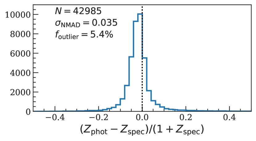
Figure 25: Spectroscopic and photometric redshifts for the 42985 sources with high-quality photo-zs and spec-zs in the 4.5 deg² region covered by the N18 forced-photometry catalog (sources identified as a broad-line AGN were excluded, see §5.1). The top panel shows the histogram of the fractional difference between the spec-zs and the photo-zs. The bottom panel shows the direct comparison between the spec-zs and the photo-zs. The black dotted lines in both panels mark the $z_{\rm spec}=z_{\rm phot}$ relation. In the bottom panel, the red dashed lines mark the $\mathopen{|}\Delta z\mathclose{|}/(1+z_{\rm spec})=0.15$ thresholds for outliers.

Table F: The main X-ray source catalog with a selection of columns. Empty or null values are marked as $-$99. The numbers listed in the second row of this table is the column numbers of the full X-ray catalog. See Appendix A for a detailed description of each column. This table is available in its entirety in machine-readable form online.

XID	RA	DEC	XPOSERR	FB_DET_ML	FB_EXP	FB_BKG	FB_SCTS	FB_FLUX	HR	LX	FLAG_RELIABLE	OIR_CATALOG	ZBEST	ZSOURCE	CLASS
(1)	(2)	(3)	(4)	(16)	(19)	(31)	(43)	(93)	(95)	(98)	(109)	(111)	(179)	(180)	(186)
XMM00000	34.200220	$-$4.035250	1.44	19.0	59076.2	1.74	83.04	8.92$\times 10^{-15}$	$-$99.0	$-$99	1	HSC	$-$99.0	$-$99	33213
XMM00001	34.200710	$-$4.933730	1.45	63.0	61051.8	1.00	82.03	8.53$\times 10^{-15}$	$-$1.0	9.66$\times 10^{43}$	1	SERVS	1.82	UDSz	32212
XMM00002	34.201450	$-$5.556720	1.96	16.4	29731.6	0.80	29.64	5.71$\times 10^{-15}$	1.0	2.64$\times 10^{42}$	1	SERVS	0.459	VIPERS	32213
XMM00003	34.201470	$-$4.499310	1.50	23.3	72553.8	1.76	72.37	5.71$\times 10^{-15}$	$-$1.0	1.47$\times 10^{43}$	1	SERVS	0.959	PRIMUS	32212
XMM00004	34.201950	$-$4.555520	0.93	316.8	87846.9	1.81	351.91	2.87$\times 10^{-14}$	$-$0.43	1.03$\times 10^{43}$	1	SERVS	0.41	SDSS	32213
XMM00005	34.202640	$-$5.690720	1.66	16.5	26430.1	1.01	52.23	1.40$\times 10^{-14}$	$-$1.0	1.81$\times 10^{44}$	1	CFHTLS	1.932	VIPERS	32213
XMM00006	34.203280	$-$4.315290	1.55	29.2	107957.7	1.79	65.42	3.16$\times 10^{-15}$	$-$99.0	$-$99	1	SERVS	$-$99.0	$-$99	33213
XMM00007	34.203750	$-$5.433790	1.77	11.3	78270.8	1.54	41.87	5.06$\times 10^{-15}$	$-$99.0	$-$99	1	VIDEO	$-$99.0	$-$99	33213
XMM00008	34.203820	$-$4.595270	1.17	114.8	83485.0	1.49	168.25	1.31$\times 10^{-14}$	$-$0.48	2.21$\times 10^{42}$	1	VIDEO	0.294	SDSS	33213
XMM00009	34.204670	$-$5.378240	1.35	57.1	93769.9	1.40	101.92	7.31$\times 10^{-15}$	$-$1.0	$-$99	1	SERVS	$-$99.0	$-$99	33213
…	…	…	…	…	…	…	…	…	…	…	…	…	…	…	…

Table G: The NWAY matching results with a selection of columns. Empty or null values are marked as $-$99. See Appendix B for a detailed description of each column. This table is available in its entirety in machine-readable form online.

XID	P_ANY	P_I	SERVS_ID	SERVS_MAG1	VIDEO_ID	VIDEO_KSMAG	CFHT_ID	CFHT_IMAG	HSC_ID	HSC_IMAG	MATCH_FLAG
(1)	(2)	(3)	(12)	(20)	(13)	(30)	(14)	(38)	(15)	(46)	(52)
XMM00000	0.00281	0.922088	701845.0	19.32	-99	-99.0	-99.0	-99	-99	-99.0	1
XMM00001	0.99867	0.990685	408032.0	19.36	644246149826	20.17	20.17	1114_171196	37485121644815869	-99.0	1
XMM00002	0.99234	0.979547	162933.0	19.72	644245967165	19.36	19.36	1114_017717	37485108759910516	-99.0	1
XMM00003	0.99192	0.987072	595262.0	18.96	644246286360	19.57	19.57	1105_044095	37485134529712709	-99.0	1
XMM00004	0.99369	0.987703	571059.0	18.82	644246268652	18.37	18.37	1105_032861	37485130234751017	-99.0	1
XMM00005	0.64455	0.993912	-99.0	-99.0	-99	-99.0	-99.0	1123_209193	37485104464927930	-99.0	1
XMM00006	0.03568	0.313800	647512.0	22.23	644246338512	23.19	23.19	1105_084654	38549431720610501	-99.0	1
XMM00007	0.01958	0.192855	-99.0	-99.0	644246003165	22.05	22.05	-99	-99	-99.0	2
XMM00007	0.01958	0.333900	-99.0	-99.0	644246382177	21.59	21.59	-99	-99	-99.0	1
XMM00007	0.01958	0.174318	-99.0	-99.0	644246413618	22.54	22.54	-99	-99	-99.0	2
XMM00008	0.99216	0.992165	-99.0	-99.0	644246255264	18.86	18.86	1105_022859	37485130234749091	-99.0	1
…	…	…	…	…	…	…	…	…	…	…	…

Table H: The photo-zs for galaxies detected in the N18 forced-photometry catalog; see Appendix C for details. Columns 1–3: VIDEO object ID, RA, and DEC (J2000). Columns 4–6: SERVS object ID, RA, and DEC (J2000). Column 7: photometric redshift. Column 8–9: Upper and lower 68% limits of the photometric redshift based on the probability distribution ($p(z)$) of the photo-zs. Note that our photo-zs correspond to the peak value of $p(z)$, and thus for a small fraction of sources, the most probable redshifts are not in the range covered by the upper and lower 68% limits. See Eq. (12) and §7.6 of Yang et al. (2014) for details. Column 10: photometric redshift quality parameter; see §5.2 for details. Column 11: Spectroscopic redshift. Null values are filled with -99. Columns 12–13: Similar to Columns 183–184 of Table A. This table is available in its entirety in machine-readable form online.

VIDEO_ID	VIDEO_RA	VIDEO_DEC	SERVS_ID	SERVS_RA	SERVS_DEC	ZPHOT	PZ_ULIM	PZ_LLIM	$Q_{z}$	ZSPEC	ZSOURCE	ZFLAG
(1)	(2)	(3)	(4)	(5)	(6)	(7)	(8)	(9)	(10)	(11)	(12)	(13)
644246417039	34.559784	-4.966628	419320	34.552429	-4.971455	0.890	0.810	0.978	0.166874	-99	…	…
644246232645	34.826369	-4.664200	463179	34.826399	-4.664191	0.729	0.628	0.805	0.025925	0.7615	VIPERS	2.5
644246414844	34.865246	-5.255360	217192	34.866427	-5.256932	1.239	0.986	1.942	0.767938	-99	…	…
644245112476	35.980791	-5.384739	79929	35.980755	-5.384734	0.799	0.644	0.982	0.351430	1.009558	PRIMUS	3
644245112310	35.990999	-5.385472	79380	35.991092	-5.385497	0.431	0.193	0.492	0.224409	0.513350	PRIMUS	4
644245264327	36.514834	-4.820542	242344	36.513482	-4.818775	0.010	0.023	0.132	0.189810	0.2036	VVDS	3
…	…	…	…	…	…	…	…	…	…	…	…	…

References

- Aihara et al. (2018) Aihara H., et al., 2018, PASJ, 70, S8
- Alam et al. (2015) Alam S., et al., 2015, ApJS, 219, 12
- Assef et al. (2013) Assef R. J., et al., 2013, ApJ, 772, 26
- Bradshaw et al. (2013) Bradshaw E. J., et al., 2013, MNRAS, 433, 194
- Brammer et al. (2008) Brammer G. B., van Dokkum P. G., Coppi P., 2008, ApJ, 686, 1503
- Brandt & Alexander (2015) Brandt W. N., Alexander D. M., 2015, The Astronomy and Astrophysics Review, 23, 1
- Broos et al. (2007) Broos P. S., Feigelson E. D., Townsley L. K., Getman K. V., Wang J., Garmire G. P., Jiang Z., Tsuboi Y., 2007, ApJS, 169, 353
- Broos et al. (2011) Broos P. S., et al., 2011, ApJS, 194, 2
- Brusa et al. (2007) Brusa M., et al., 2007, ApJS, 172, 353
- Cappelluti et al. (2007) Cappelluti N., et al., 2007, ApJS, 172, 341
- Cappelluti et al. (2009) Cappelluti N., et al., 2009, A&A, 497, 635
- Chiappetti et al. (2005) Chiappetti L., et al., 2005, A&A, 439, 413
- Civano et al. (2016) Civano F., et al., 2016, ApJ, 819, 62
- Coil et al. (2011) Coil A. L., et al., 2011, ApJ, 741, 8
- Dawson et al. (2013) Dawson K. S., et al., 2013, AJ, 145, 10
- Diehl et al. (2014) Diehl H. T., et al., 2014, in Observatory Operations: Strategies, Processes, and Systems V. p. 91490V, doi:10.1117/12.2056982
- Donley et al. (2012) Donley J. L., et al., 2012, Astrophys. J., 748, 142
- Driver & Robotham (2010) Driver S. P., Robotham A. S. G., 2010, MNRAS, 407, 2131
- Evans et al. (2010) Evans I. N., et al., 2010, ApJS, 189, 37
- Falocco et al. (2017) Falocco S., et al., 2017, A&A, 608, A32
- Franzen et al. (2015) Franzen T. M. O., et al., 2015, MNRAS, 453, 4020
- Garilli et al. (2014) Garilli B., et al., 2014, A&A, 562, A23
- Georgakakis & Nandra (2011) Georgakakis A., Nandra K., 2011, MNRAS, 414, 992
- Hasinger et al. (1998) Hasinger G., Burg R., Giacconi R., Schmidt M., Trumper J., Zamorani G., 1998, A&A, 329, 482
- Hasinger et al. (2007) Hasinger G., et al., 2007, ApJS, 172, 29
- Hudelot et al. (2012) Hudelot P., et al., 2012, VizieR On-line Data Catalog: II/317. Originally published in: SPIE Conf. 2012, 2317
- Jarvis et al. (2012) Jarvis M. J., et al., 2012, MNRAS, 428, 1281
- Jarvis et al. (2017) Jarvis M. J., et al., 2017, preprint, (arXiv:1709.01901)
- Kelson et al. (2014) Kelson D. D., et al., 2014, ApJ, 783, 110
- Kim et al. (2007) Kim M., Wilkes B. J., Kim D., Green P. J., Barkhouse W. A., Lee M. G., Silverman J. D., Tananbaum H. D., 2007, ApJ, 659, 29
- Klypin et al. (2016) Klypin A., Yepes G., Gottlöber S., Prada F., Heß S., 2016, MNRAS, 457, 4340
- LaMassa et al. (2016) LaMassa S. M., et al., 2016, ApJ, 817, 172
- Lacy et al. (2004) Lacy M., et al., 2004, Astrophys. J. Suppl. Ser., 154, 166
- Lang et al. (2016) Lang D., Hogg D. W., Mykytyn D., 2016, The Tractor: Probabilistic astronomical source detection and measurement, Astrophysics Source Code Library (ascl:1604.008)
- Le Fevre et al. (2013) Le Fevre O., et al., 2013, A&A, 559, A14
- Liu et al. (2016) Liu Z., et al., 2016, MNRAS, 459, 1602
- Lonsdale et al. (2003) Lonsdale C. J., et al., 2003, PASP, 115, 897
- Luo et al. (2010) Luo B., et al., 2010, ApJS, 187, 560
- Luo et al. (2017) Luo B., et al., 2017, ApJS, 228, 2
- Mainieri et al. (2007) Mainieri V., et al., 2007, ApJS, 172, 368
- Marchesi et al. (2016) Marchesi S., et al., 2016, ApJ, 817, 34
- Mateos et al. (2009) Mateos S., Saxton R. D., Read A. M., Sembay S., 2009, A&A, 496, 879
- Mateos et al. (2013) Mateos S., Alonso-Herrero A., Carrera F. J., Blain A., Severgnini P., Caccianiga A., Ruiz A., 2013, Mon. Not. R. Astron. Soc., 434, 941
- Mauduit et al. (2012) Mauduit J.-C., et al., 2012, PASP, 124, 714
- McLure et al. (2013) McLure R. J., et al., 2013, MNRAS, 428, 1088
- Meneux et al. (2009) Meneux B., et al., 2009, A&A, 505, 463
- Menzel et al. (2016) Menzel M. L., et al., 2016, MNRAS, 457, 110
- Momcheva et al. (2016) Momcheva I. G., et al., 2016, ApJS, 225, 27
- Moster et al. (2011) Moster B. P., Somerville R. S., Newman J. A., Rix H.-W., 2011, ApJ, 731, 113
- Nyland et al. (2017) Nyland K., et al., 2017, ApJS, 230, 9
- Oliver et al. (2012) Oliver S. J., et al., 2012, MNRAS, 424, 1614
- Pacaud et al. (2006) Pacaud F., et al., 2006, MNRAS, 372, 578
- Paolillo et al. (2017) Paolillo M., et al., 2017, MNRAS, 471, 4398
- Park et al. (2006) Park T., Kashyap V. L., Siemiginowska A., van Dyk D. A., Zezas A., Heinke C., Wargelin B. J., 2006, ApJ, 652, 610
- Patel et al. (2015) Patel S. G., Kelson D. D., Williams R. J., Mulchaey J. S., Dressler A., McCarthy P. J., Shectman S. A., 2015, ApJ, 799, L17
- Pierre et al. (2016) Pierre M., et al., 2016, A&A, 592, A1
- Pineau et al. (2017) Pineau F.-X., et al., 2017, A&A, 597, A89
- Polletta et al. (2007) Polletta M., et al., 2007, ApJ, 663, 81
- Ranalli et al. (2013) Ranalli P., et al., 2013, A&A, 555, A42
- Ranalli et al. (2015) Ranalli P., et al., 2015, A&A, 577, A121
- Rosen et al. (2016) Rosen S. R., et al., 2016, A&A, 590, A1
- Salvato et al. (2011) Salvato M., et al., 2011, ApJ, 742, 61
- Salvato et al. (2017) Salvato M., et al., 2017, eprint arXiv:1705.10711
- Skelton et al. (2014) Skelton R. E., et al., 2014, ApJS, 214, 24
- Skibba et al. (2014) Skibba R. A., et al., 2014, ApJ, 784, 128
- Skrutskie et al. (2006) Skrutskie M. F., et al., 2006, AJ, 131, 1163
- Stark et al. (1992) Stark A. A., Gammie C. F., Wilson R. W., Bally J., Linke R. A., Heiles C., Hurwitz M., 1992, ApJS, 79, 77
- Stern et al. (2005) Stern D., et al., 2005, Astrophys. J., 631, 163
- Stern et al. (2012) Stern D., et al., 2012, Astrophys. J., 753, 30
- Sutherland & Saunders (1992) Sutherland W., Saunders W., 1992, MNRAS, 259, 413
- Takada et al. (2014) Takada M., et al., 2014, PASJ, 66, R1
- Tanaka et al. (2018) Tanaka M., et al., 2018, PASJ, 70, S9
- Tonry et al. (2012) Tonry J. L., et al., 2012, ApJ, 745, 42
- Ueda et al. (2008) Ueda Y., et al., 2008, ApJS, 179, 124
- Vaccari (2015) Vaccari M., 2015, in The Many Facets of Extragalactic Radio Surveys: Towards New Scientific Challenges. p. 27 (arXiv:1604.02353)
- Vaccari (2016) Vaccari M., 2016, The Universe of Digital Sky Surveys, 42, 71
- Vaccari et al. (2016) Vaccari M., et al., 2016, in Proceedings of the 4th Annual Conference on High Energy Astrophysics in Southern Africa (HEASA 2016). 25-26 August, 2016. South African Astronomical Observatory (SAAO), Cape Town, South Africa. Online at http://pos.sissa.it/cgi-bin/reader/conf.cgi?confid=27, id.26. p. 26 (arXiv:1704.01495)
- Warren et al. (2007) Warren S. J., et al., 2007, arXiv e-prints astro-ph/0703037,
- Watson et al. (2008) Watson M. G., et al., 2008, A&A, 493, 339
- Xue (2017) Xue Y. Q., 2017, New Astron. Rev., 79, 59
- Xue et al. (2011) Xue Y. Q., et al., 2011, ApJS, 195, 10
- Xue et al. (2016) Xue Y. Q., Luo B., Brandt W. N., Alexander D. M., Bauer F. E., Lehmer B. D., Yang G., 2016, ApJS, 224, 15
- Yang et al. (2014) Yang G., et al., 2014, ApJS, 215, 27
- Yang et al. (2016) Yang G., et al., 2016, ApJ, 831, 145
- Yang et al. (2018) Yang G., et al., 2018, MNRAS, 475, 1887
- York et al. (2000) York D. G., et al., 2000, Astron. J., 120, 1579
- Zheng et al. (2017) Zheng X. C., et al., 2017, ApJ, 849, 127
- de la Torre et al. (2010) de la Torre S., et al., 2010, MNRAS, 409, 867