GPI spectra of HR 8799 c, d, and e from 1.5 to 2.4$\mu m$ with KLIP Forward Modeling

Abstract

We explore KLIP forward modeling spectral extraction on Gemini Planet Imager coronagraphic data of HR 8799, using PyKLIP and show algorithm stability with varying KLIP parameters. We report new and re-reduced spectrophotometry of HR 8799 c, d, and e in H & K bands. We discuss a strategy for choosing optimal KLIP PSF subtraction parameters by injecting simulated sources and recovering them over a range of parameters. The K1/K2 spectra for HR 8799 c and d are similar to previously published results from the same dataset. We also present a K band spectrum of HR 8799 e for the first time and show that our H-band spectra agree well with previously published spectra from the VLT/SPHERE instrument. We show that HR 8799 c and d show significant differences in their H & K spectra, but do not find any conclusive differences between d and e or c and e, likely due to large error bars in the recovered spectrum of e. Compared to M, L, and T-type field brown dwarfs, all three planets are most consistent with mid and late L spectral types. All objects are consistent with low gravity but a lack of standard spectra for low gravity limit the ability to fit the best spectral type. We discuss how dedicated modeling efforts can better fit HR 8799 planets’ near-IR flux and discuss how differences between the properties of these planets can be further explored.

1 Introduction

Directly imaged planets present excellent laboratories to study the properties of the outer-architectures of young solar systems. Near-infrared spectroscopic follow-up can constrain atmospheric properties including molecular absorption, presence of clouds, and non-equilibrium chemistry (Barman et al., 2011; Konopacky et al., 2013; Marley et al., 2012). Composition, especially in relation to the host star is an important probe of physical processes and formation history (Öberg et al., 2011).

HR 8799 is a 1.5 $M_{\odot}$ star (Gray & Kaye, 1999; Baines et al., 2012) located at a distance of $39.4\pm 1.0pc$ (van Leeuwen, 2007) with an estimated age of $\sim 30Myr$ (Moór et al., 2006; Marois et al., 2008; Hinz et al., 2010; Zuckerman et al., 2011; Baines et al., 2012; Malo et al., 2013) based on it’s likely membership in the Columba association. It contains multiple imaged planets b, c, d, and e (Marois et al., 2008, 2010b) witthat lie between 10 and 100 AU separations from the host star. Lavie et al. (2017) show the inner 3 planets fall within the $\mathrm{H_{2}O}$ and $\mathrm{CO_{2}}$ ice lines based on a vertically isothermal, passively irradiated disk model. Konopacky et al. (2013) point out that in this region non-stellar C and O abundances are available to accrete onto a planetary core, and that the measured abundances of HR 8799 planets could help distinguish between core-accretion scenario and gravitational instability, which is expected to produce stellar-abundances.

HR 8799 has been a testbed for detection techniques (e.g., Lafrenière et al., 2009; Soummer et al., 2011), astrometric monitoring and dynamical studies (Fabrycky & Murray-Clay, 2010; Soummer et al., 2011; Pueyo et al., 2015; Konopacky et al., 2016; Zurlo et al., 2016; Wertz et al., 2017), atmospheric characterization (Janson et al., 2010; Bowler et al., 2010; Hinz et al., 2010; Barman et al., 2011; Madhusudhan et al., 2011; Currie et al., 2011; Skemer et al., 2012; Marley et al., 2012; Konopacky et al., 2013; Ingraham et al., 2014; Barman et al., 2015; Rajan et al., 2015; Bonnefoy et al., 2016), and even variability (Apai et al., 2016). Studying the properties of multiple planets in the same system presents a unique opportunity for understanding its formation, by studying dynamics and composition as a function of mass and semi-major axis.

Spectrophotometry and moderate resolution spectroscopy have provided a detailed view into the atmospheres of the HR 8799 companions. Water and carbon monoxide absorption lines have been detected in the atmospheres of planets b and c, with methane absorption additionally detected in b (Barman et al., 2011; Konopacky et al., 2013; Barman et al., 2015). To account for the discrepancy between the spectra of b and c and those of field brown dwarfs, various studies based on near-IR observations from 1-5$\mu$m have proposed the presence of clouds (e.g. Marois et al., 2008; Hinz et al., 2010; Madhusudhan et al., 2011), disequilibrium chemistry to explain an absence of methane absorption (Barman et al., 2011; Konopacky et al., 2013), and non-solar composition (Lee et al., 2013). However, some work suggests that prescriptions of disequilibrium chemistry, non-solar composition, and/or patchy atmospheres may not play an important role for the d, e planets (e.g. Bonnefoy et al., 2016), which appear consistent with dusty late-L objects based on their YJH spectra and SEDs, and can be modeled with atmospheres that do not contain these features. K band spectra are especially sensitive to atmospheric properties and composition and can probe the presence of methane and water. HR 8799 b, c, and d have shown a lack of strong methane absorption in the K-band spectra (Bowler et al., 2010; Barman et al., 2011; Currie et al., 2011; Konopacky et al., 2013; Ingraham et al., 2014), inconsistent with field T-type brown dwarfs.

Stellar PSF subtraction algorithms that take advantage of angular and/or spectral diversity, while powerful for removing the stellar PSF, result in self-subtraction of the signal of interest, which can bias the measured astrometry and photometry (Marois et al., 2010a). Self-subtraction biases in the signal extraction are commonly avoided by injecting negative simulated planets in the data and optimizing over the residuals (e.g., Lagrange et al., 2010). For multi-wavelength IFU data, template PSFs of representative spectral types can be used to optimize the extraction/detection (Marois et al., 2014; Gerard & Marois, 2016; Ruffio et al., 2017). An analytic forward model of the perturbation of the companion PSF due to self-subtraction effects can be a more efficient approach that is less dependent on the template PSF and algorithm parameters (Pueyo, 2016).

In this paper we present H & K spectra of HR 8799 c, d, and e obtained with the Gemini Planet Imager (GPI). We use Karhunen Loéve Image Projection (KLIP) for PSF subtraction (Soummer et al., 2011) with the forward model formalism demonstrated in Pueyo (2016). In §2 we describe our observations and data reduction. This is followed by a brief description of KLIP forward modeling (hereafter KLIP-FM) and discussion of the stability of our extracted signal with varying KLIP parameters. In §3 we present our recovered spectra alongside previous results (Oppenheimer et al., 2013; Ingraham et al., 2014; Zurlo et al., 2016; Bonnefoy et al., 2016), and discuss consistencies and discrepancies. We also describe a method to calculate the similarity of the three extracted spectra and discuss our findings. We compare a library of classified field and low gravity brown dwarfs to our H and K spectra in §4 and report best fit spectral types. Finally, we discuss a few different atmospheric models and their best fits to our spectra in §5. We summarize and discuss these results in §6. In Appendix A we show our detail residuals between the processed data and the forward models. Appendix B we compare the forward model extraction described in this study with other algorithms. In Appendix C we show planet comparisons by individual bands. We provide our spectra in Appendix D.

2 Observations and Data Reduction

2.1 GPI Observations and Datacube Assembly

Table 1: Summary of observations

DATE	Band	$N_{frame}$	$\mathrm{t_{frame}}$	$\Delta\mathrm{PA}$	Airmass	Seeing
2013/11/17	K1	24	90 $s$	$17.1^{o}$	1.62	$0\farcs 98$
2013/11/18	K2	20	90 $s$	$9.7^{o}$	1.62	$0\farcs 72$
2016/09/19	H	60	60 $s$	$20.9^{o}$	1.61	$0\farcs 97$

HR 8799 was observed with the Gemini Planet Imager Integral Field Spectrograph (IFS) (Macintosh et al., 2014) with its K1 and K2 filters on 2013 November 17 (median seeing $0\farcs 97$) and November 18 (median seeing 0.75 arcsec), respectively, during GPI’s first light. The data were acquired with a continuous field of view (FOV) rotation near the meridian transit to achieve maximum FOV rotation suitable for ADI processing (Marois et al., 2006a). Conditions are described in detail in Ingraham et al. (2014). During the last 10 exposures of the K1 observations cryocooler power was decreased to 30% to reduce vibration, and the last 14 exposures of the K2 observations had the cryocooler power decreased. Since commissioning linear-quadratic-Gaussian control has been implemented (Poyneer et al., 2016) and the cryocooling system has been upgraded with active dampers to mitigate cryocooler cycle vibrations. HR 8799 was observed again on September 19 2016 in GPI’s H-band (median seeing $0\farcs 97$) as a part of the GPI Expolanet Survey (GPIES) with the updated active damping system. Planet b falls outside the field of view in these data. Table 1 summarizes all GPI observations of HR 8799 used in this study.

Datacube assembly was performed using the GPI Data Reduction Pipeline (DRP) (GPI instrument Collaboration, 2014; Perrin et al., 2014, 2016). Wavelength calibration for the K1 and K2 data was done using a Xenon arc lamp and flexure offset adjusted manually (Wolff et al., 2014). Bad pixels were corrected and dark and sky frames were subtracted from the raw data. The raw detector frames were assembled into spectral datacubes. Images were corrected for distortion (Konopacky et al., 2014) and high pass filtered. H-band datacube reduction followed a similar procedure, except that flexure offsets were automatically determined based on contemporaneous arc lamp images. Wang et al. (2018) contains a thorough description of standard data reduction procedures.

The instrument transmission function was calibrated using the GPI grid apodizer spots, which place a copy of the stellar PSF in four locations in the image (Sivaramakrishnan & Oppenheimer, 2006; Marois et al., 2006b). These fiducial satellite spots are used to convert raw data counts to contrast units and to register and demagnify the image (Maire et al., 2014; Wang et al., 2014).

2.2 KLIP forward modeling for unbiased spectra

Stellar PSF subtraction is performed by constructing an optimized combination of reference images with KLIP (For a complete description see Soummer et al., 2012). Reference images are assembled from the full dataset to take advantage of both angular and spectral diversity. The KL basis, $Z_{k}$ is formed from the covariance matrix of the reference images and projected onto the data $I(n)$ to subtract the Stellar PSF:

$$S=\sum(I(n)-\sum_{k=1}^{k_{klip}}<I,Z_{k}>_{S}Z_{k}(n))$$ (1)

where $S$ is the klipped data and $Z_{k}$ is determined by the reference library selection criteria. To account for over- and self- subtraction of the companion signal we use the approach detailed in Pueyo (2016) to forward model the signal in PSF-subtracted data to recover an unbiased spectrum. The forward model is constructed by perturbing the covariance matrix of the reference library to account for a faint companion signal and propagating this through the KLIP algorithm for additional terms, as we show in Equation 2. Over- and self-subtraction effects are accounted for in the forward model by projecting a model of the PSF, $F_{model}$, onto the unperturbed KL basis, $Z_{k}$, (over-subtraction) and projecting the PSF model onto the the KL basis perturbation (self-subtraction), where the KL basis perturbation, $\Delta Z_{k}$, is a function of the unperturbed KL basis, $Z_{k}$, and the PSF model, $F_{model}$. The forward model is constructed by the terms that are linear in the planet signal:

$$FM = \sum F_{model}$$ (2)

$$- \sum<F_{model},Z_{k}>Z_{k}$$

$$- \sum<Z_{k},Z_{k}>\Delta Z_{k}-\sum<Z_{k},\Delta Z_{k}>Z_{k}$$

For the analysis presented in this paper, the PSF model, $F_{model}$, is constructed from the satellite spots.

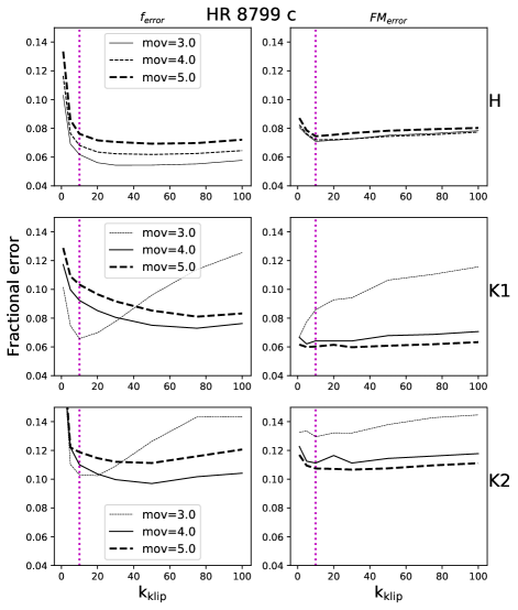
Figure 1: Residual errors over a range of KLIP-FM parameters for HR 8799 c. Left: Difference between the injected spectrum at the planet location and the recovered spectra of simulated injections, normalized by the recovered spectrum (Equation 4). Right: The residual error of the forward model normalized by the sum of the pixels. (Equation 2.2). The solid line denotes the chosen exclusion criterion, or $mov$ value (in pixels). The number of KL components used, $k_{klip}$, denoted by the vertical dotted line, is chosen in a region where $f_{error}$ is decreasing at the selected value of $mov$.

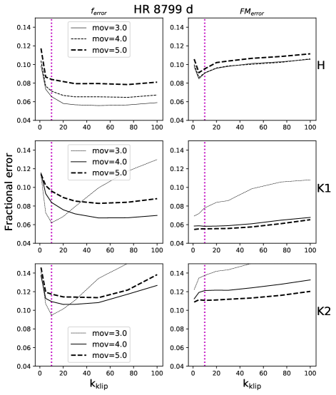
Figure 2: Same as Figure 1, but for HR 8799 d. The intersection of the solid curve and verticle dotted line denote our choice of parameters.

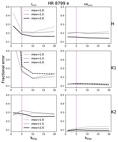
Figure 3: Same as Figure 1, but for HR 8799 e. The intersection of the solid curve and verticle dotted line denote our choice of parameters.

After computing the forward model, the spectrum is recovered by solving the inverse problem for $f_{\lambda}$:

$$f_{\lambda}\cdot FM=S$$ (3)

where $S$ is the stellar PSF-subtracted data processed with KLIP, as in Equation 1. This assumes the relative astrometry has already been calculated. Using the approximate contrast summed over the bandpass for each object we run Bayesian KLIP Astrometry (Wang et al., 2016) to measure the astrometry of each planet in the different datasets first. The improved position reduces residuals between the forward model containing the optimized spectrum and the PSF-subtracted data. The procedures and documentation are available in the PyKLIP package.

PCA-based PSF subtraction, especially which includes the signal of the companion as in the case of ADI and Simultaneous Spectral Differential Imaging (SSDI), will bias the extracted spectrum (Marois et al., 2006c; Pueyo et al., 2012). This bias is often seen as a sensitivity to algorithm parameters. We run KLIP Forward Modeling (KLIP-FM) spectral extraction considering the effect of two KLIP parameters, the KLIP cuttoff $k_{klip}$, which sets the number of KL modes used for the subtraction, and movement (or aggressiveness), $mov$, which defines the maximum allowed level of overlap between the planets position in a given image and other images selected for its reference library. See Ruffio et al. (2017) for a more formal definition. We vary these parameters as a proxy for understanding how biased and noisy our extraction is. As in Pueyo (2016) we expect this forward modeling approach to be less sensitive to changing algorithm parameters than regular PCA-style subtractions, and overall this is what we observe. However, there is still some 2nd-order dependence either due to the model being wrong or noise in the image.

We examine how the spectral extraction results vary with algorithm parameters through two measures of error, error in the spectrum extraction $f_{error}$ and residual error around the location of the signal $FM_{error}$. To measure error in the spectral extraction, artificial signals are inserted into the data. We simulate 11 artificial signals evenly distributed (30 deg apart) in an annulus at the same separation but avoiding the position angle of the planet. The artificial sources are simulated with spectra corresponding to the spectrum measured from the planet with KLIP-FM. We define $f_{error}$ as

$$f_{error}=\frac{1}{N_{\lambda}}\sum_{\lambda}^{N_{\lambda}}\sqrt{\frac{\sum_{i}^{N_{sim}}(f_{\lambda}-f^{\prime}_{\lambda,i})^{2}}{N_{sim}f_{\lambda}^{2}}}$$ (4)

where $f_{\lambda}$ is the spectrum recovered at the location of the planet and $f^{\prime}_{\lambda,i}$ is the spectrum recovered for the $i$th artificial source of total $N_{sim}$ sources. Our spectral datacubes contain $N_{\lambda}=37$ wavelength slices per band. We define the residual error, $FM_{error}$, as the square root of the sum of the residual image pixels squared divided by the sum of the klipped image of the planet squared. The residual is calculated inside a region with a radius of 4 pixels centered on the planet.

$$R = \sum_{\lambda}^{N_{\lambda}}S_{\lambda}-FM_{\lambda},$$

$$FM_{error} = \sqrt{\frac{\sum_{pix}R^{2}}{\sum_{pix}{S^{2}}}}$$ (5)

Appendix A contains the full residuals in the region around each planet for each band.

Figures 1, 2, and 3, for planets c, d, and e respectively, display the spectrum error (left) and residual error (right) for the range of investigated KLIP parameters. We see that the error converges as $k_{klip}$ increases as demonstrated in Pueyo (2016), when the model is capturing the signal. In certain cases when the model is wrong, the error does not converge as we see for planets c and d K-band data when $mov=3$. These metrics show the stability of of the forward model solution with KLIP parameters. The solid line plotted in each panel represents the value of $mov$ chosen for the final spectrum, with the other values of $mov$ represented in dashed lines of varying thickness. The dotted vertical magenta line represents the chosen value of $k_{klip}$. For planet e we excluded the two closest simulated sources to avoid contamination from the real planet signal.

We choose KLIP parameters that minimize the $f_{error}$ term and prefer solutions with smaller value of $k_{klip}$ that occur before the minimum. We also check that the residual error $FM_{error}$ stays relatively flat. As demonstrated in Pueyo (2016) the forward model starts to fail for larger $k_{klip}$ when the signal is bright. The error in the residual is generally close to the spectrum error, $f_{error}$, except in the K1 and K2 reductions of e, when the spectrum error could be reflecting more residual speckle noise. The spectrum error term is fairly well behaved for all three planets, in general flattening with $k_{klip}$. The H band data, for which our reduction show the most stable behavior with KLIP parameters, has more rotation and was taken after several upgrades to the instrument. The behavior of the two error metrics for HR 8799 e improved when wavelength slices from the band edges were removed prior to PSF subtraction.

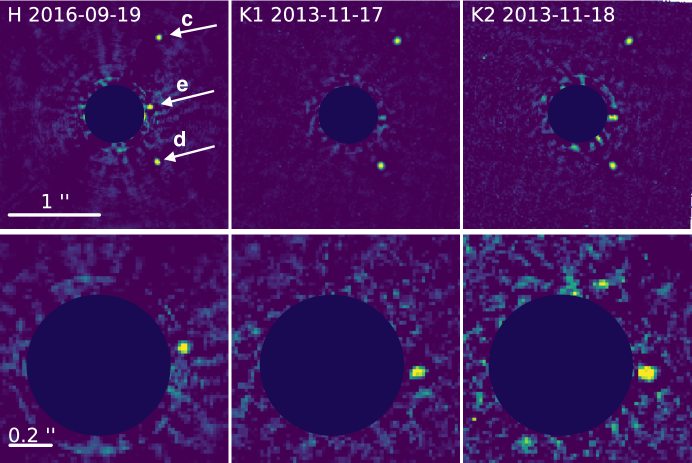
Figure 4: Top: Our standard KLIP subtracted cubes with $mov$ = 3 pixels. Bottom: Subtracted cubes with $mov$ = 1 pixel. The data are zoomed in to highlight HR 8799. The H band data quality is higher due to larger field rotation. We see the relative position difference of planet e due to orbital motion between the 2013 (K band) and 2016 (H band) epochs.

For HR 8799 c and d we note that most of the parameter combinations yield a similar level of error, within a few percent. Changing the klip parameters near our chosen values does not have a large effect on the spectrum. For HR 8799 e the bias is generally higher (note the scale in Figure 3). This is reflected in the larger error bars for e reported in our final spectrum. We display our collapsed datacubes reduced through PyKLIP in Figure 4 showing a less aggressive reduction (larger $mov$) used to extract spectra of HR 8799 c and d in the top panel, and more aggressive reduction (smaller $mov$, including more images in the reference library) used to extract the spectrum of HR 8799 e in the bottom row.

3 Results using optimized KLIP parameters

After inspecting an initial reduction with all data, we remove slices at the ends of each cube where the signal is low (due to low filter throughput at band edges) and re-rerun our reduction. We take this step to avoid biasing the spectrum extracted in Equation 3 with datacube slices that contain no signal. KLIP errors are computed from the standard deviation of the simulated source recovery at each wavelength channel. Errorbars displayed reflect the standard deviation of the spectrum recovered from simulated sources and the uncertainty in the satellite spot flux, calculated from measuring the variation of the spot flux photometry in this data.

We find that in some parts of the spectrum, the scatter in flux of the recovered injected signals is not symmetric about the injected spectrum, which indicates that the model is slightly wrong to a scaling factor. This effect is typically on the order of $5-10\%$ and is most obvious between $2.0-2.2\mu m$ for c and d, and at the short wavelength edge of K1 for e. In Figure 5 we show the the recovered spectrum and the recovered artifical sources. To account for bias in spectral extraction, we have adjusted the spectrum by a scaling term that accounts for the flux loss, which is the factor between the recovered spectrum and the mean spectrum recovered from the simulated sources,

$$F_{\lambda}=\frac{f_{\lambda,k}}{\sum f_{sim\lambda,k}/N_{sim}}$$ (6)

for the $\mathrm{k_{th}}$ planet at each wavelength slice, $\lambda$. Where the scatter is more symmetric (such as in all the H-band datasets) the model is correctly accounting for the flux and the adjusted spectrum matches the initial reduction. All following figures and calculations in this paper use the adjusted spectrum.

As in Bonnefoy et al. (2016), we use a Kurucz spectrum at 7500K, matched to the photometry of HR 8799 A, to convert contrast to flux. We display results for the best KLIP parameters in Figure 6, adjusting our spectrum for c as indicated in Figure 5. Cyan points represent Palomar/P1640 data from Oppenheimer et al. (2013), which are scaled from normalized flux to match the rest of the points plotted. Dark blue lines for c and d panels are the K band spectra from the same dataset previous published in Ingraham et al. (2014). In black are SPHERE/IFS YJH spectra published by Zurlo et al. (2016) and blue squares show SPHERE/IRDIS photometry.

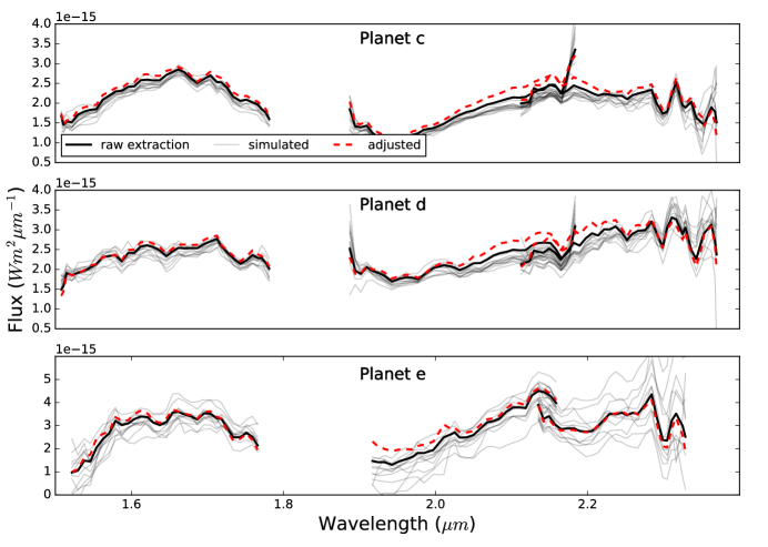
Figure 5: Resulting flux at 10pc of KLIP-FM spectrum extraction for each planet (solid black line) and recovery of artificial sources (gray lines), simulated with the matching spectrum. Increases in flux at the edges of the K1 band, where the filter throughput is low, are not significant. These are not seen in the case of e since these datta were processes without the wavelength slices at the edge of the band. The red dotted line shows the adjusted spectrum applying the flux loss factor in Equation 6.

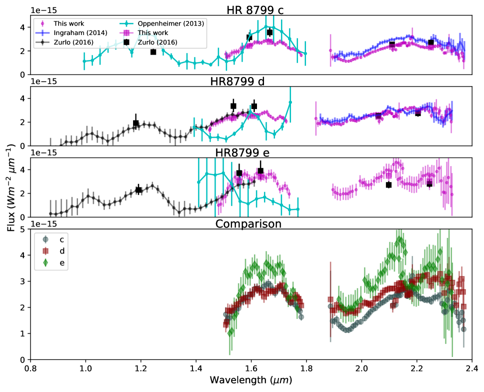
Figure 6: Spectra recovered with KLIP FM for HR 8799 c, d, and e showing flux at 10pc. Overplotted are the original GPI K-band spectra of c and d for the same dataset in dark blue (Ingraham et al., 2014), YJH spectra from Palomar/P1640 (Oppenheimer et al., 2013) (KLIP reduction) in cyan points, YJH spectra and JHK photometry using the VLT/SPHERE instrument(Zurlo et al., 2016) in black points and squares. The P1640 points are scaled from normalized flux units to match our data for this comparison. The bottom panel shows a comparison of our three recovered spectra.

Our K-band spectrum for HR 8799 e changed the most with varying KLIP parameters. We note a discrepancy between the overlapping edges of our K1 and K2 spectra for e. This is unlikely to be a calibration error since it is not seen in the cases of the c and d spectra (except at the very edges of the band where the transmission is very low. Based both on photometry from Zurlo et al. (2016) and our residual errors (see Appendix A) the K1 fluxes may not be correct. We suspect the K2 reduction is more representative of the true spectrum. We note that our K2 spectrum of e more closely resembles that of d than K1.

We find very similar morphology as the previously published spectra for c and d, although slightly lower flux in the case of c. Since these planets are so bright we may still be over-subtracting, if the linear approximation in the forward model is not appropriate, as described in Pueyo (2016). Our results are consistent with SPHERE/IRDIS K1 & K2 photometery within errorbars, but systematically lower. Ingraham et al. (2014) noted the K-band spectra in particular, combined with photometry at 3 and 4 $\mu$m showed a lack of methane absorption, and our re-reduction is consistent. They noted the flatter spectrum for d, which also appears to be the case for our new H-band spectra compared with c and e.

The SPHERE IRDIS H-band photometry are discrepant with our result. However, these photometry are also discrepant with the SPHERE IFS spectra. Our KLIP-FM H-band spectra for d and e are in good agreement with those obtained from the SPHERE IFS, within error bars. Towards the center of H band we see a slight dip in the spectrum for HR 8799 e, between 1.6 and 1.7 $\mu$m, which is not seen in the SPHERE IFS spectrum. However, there due to correlated noise, this may not be a real effect. Y and J observations of HR 8799 with GPI will improve the comparison and provide a complete YJHK spectra on the same instrument.

3.1 Comparison of c, d, and e

Differences between the three spectra could show evidence of varying atmospheric composition and formation histories, or first order physical effects such as clouds, temperature, and gravity. In the bottom panel of Figure 6 we plot all three spectra on the same axes. The H band spectrum of e appears to be most discrepant from the other two, and there are differences between all three in K1-K2. We note that our K1 and K2 spectra for e do not match in the overlap region around 2.18 $\mu m$. This is only the case for e, which could indicate that is it not due to the algorithm or flux calibration, but more speckle residuals close in. The residual images in Appendix A also show a possible speckle influencing the forward model solution for K1 data. The short wavelength edge of K2 suggests the spectrum is more similar to that of d.

These small differences motivate a more quantitative comparison. We compute $\chi^{2}_{i,j}$ between each spectrum and a spectrum drawn randomly from its error:

$$\chi^{2}_{i,j}=\frac{1}{N_{\lambda}-1}(f_{i}-f_{j}^{*})^{T}Cov_{i}^{-1}(f_{i}-f_{j}^{*})$$ (7)

where $f$ is the spectrum of the $i$th object normalized by its sum, and $f_{j}^{*}$ is a spectrum drawn randomly from the sum-normalized spectrum of the $j$th assuming Gaussian errors, taking into account covariance $Cov_{j}$ (where the errors are scaled by the same normalization factor). $Cov_{i}$ and $Cov_{j}$ are the covariance matrices of the $i$th and $j$th planets computed as described in Greco & Brandt (2016) and De Rosa et al. (2016). Here we draw $f_{j}^{*}$ and compute this statistic $10^{5}$ times and compare the resulting distributions for each planet. We consider the full H-K spectrum so that relative flux between bands is preserved.

We plot the histograms of $\chi^{2}$ in Figure 7. We compare the $\chi^{2}$ distribution of each spectrum with one drawn randomly from the same spectrum ($i=j$ case, diagonals), with the $\chi^{2}$ distribution of each spectrum compared to one drawn randomly from the other two ($i\neq j$ case, off-diagonals). The results show a discrepancy between c and d to $>5\sigma$. There is a less significant discrepancy between HR 8799 c and e and between d and e. While the $\chi^{2}$ distributions of c-e and c-c and the distributions of d-e and d-d appear distinct, there is still some overlap in the $\chi^{2}$ distributions of e-e and e-c and between e-e and e-d. This lack of symmetry is likely due to larger errorbars of the HR 8799 e spectrum. These results show a discrepancy between e and c to $\sim 1.8\sigma$ and between e and d to $\sim 1.2\sigma$. Reducing the errors for the planet e spectrum could improve this comparison. Resolving the discrepancy in the spectrum of e between K1 and K2 bands edges should also improve this comparison.

We repeated the same comparison for each of H, K1, and K2 bands separately, where the spectra and errors are normalized within each band. We show the detailed results in Appendix C. In this case we do not find the same differences between the spectra. This indicates that the relative level of flux between bands is the dominant effect.

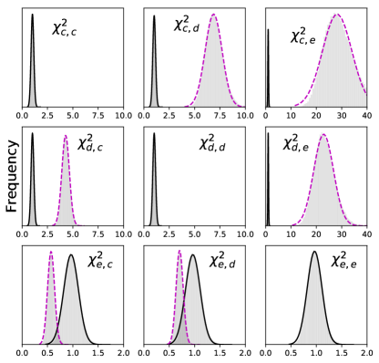
Figure 7: A cross-comparison of all three planets showing the distribution of $\chi^{2}_{i,j}$ (defined in Equation 7). The diagonal shows each spectrum compared with $10^{5}$ random draws from itself within the error bars. These, in solid outline are repeated for each panel in the same row. The off-diagonal panels also show the comparison with random draws from a different object spectrum, as indicated. These show clear ($>5\sigma$) discrepancy between c and d planets.

4 Comparison to field objects

We compare our results with known field objects as described in Chilcote et al. (2017). We compare our H & K spectrophotometry with a library of $\sim 1600$ spectra for M,L and T-dwarf field objects. These are compiled from the SpeX Prism library (Burgasser, 2014), the IRTF Spectral Library (Cushing et al., 2005), the Montreal Spectral Library (Gagné et al., 2015; Robert et al., 2016), and from Allers & Liu (2013). Each spectrum and uncertainty was binned to the spectral resolution of GPI ($R\sim 45-80$ increasing from H to K2). We convolve the spectrum with a Gaussian function of width matching the resolution for that band. The uncertainties are normalized by the effective number of spectral channels within the convolution width. Spectra that are incomplete in the GPI filter coverage are excluded from the fit.

Spectral type classifications were obtained from various literature sources, specified for individual objects. For objects that had both optical and near-IR spectral types, the near-IR spectral type was used. Gravity classifications were assigned from the literature as either old field dwarfs ($\alpha$, FLD-G), intermediate surface gravity ($\beta$, INT-G), or low surface gravity, such as typically seen in young brown dwarfs ($\gamma$, $\delta$). Several studies (Kirkpatrick, 2005; Kirkpatrick et al., 2006; Cruz et al., 2009) outline the $\alpha$, $\beta$, $\gamma$ classification scheme, including an additional $\delta$ classification from Kirkpatrick (2005) to account for even lower gravity features, based on optical spectra. FLD-G, INT-G, VL-G, based on Near-IR spectra, follows (Allers & Liu, 2013). The results between the two classification schemes are correlated (as discussed in Allers & Liu, 2013) but do not always match.

First we compare our spectra with those of each object in the compiled library, separately for H and K1-K2 bands. We compute reduced $\chi^{2}$ using the binned spectra of comparison objects. The results for each of HR 8799 c, d, and e are shown in Figure 8. Spectral standards are marked for gravity classification where the classification is known.

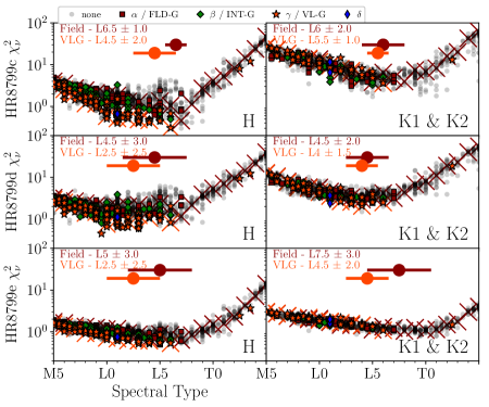
Figure 8: We plot $\chi^{2}_{\nu}$ between our GPI spectrum and each object in the spectral libraries described, as a function of spectral type of field objects for each planet. From top to bottom we plot planets c, d, and e. The left shows $\chi^{2}$ for H band, the right shows the $\chi^{2}$ for combined K1, K2 bands. The large red and orange points at the top of each panel represent the mean and $1-\sigma$ error for the best fit SED for field and VLG objects, respectively. We indicate gravity classification by the legend at the top. Spectral standards for FLD-G (Burgasser, 2014; Kirkpatrick et al., 2010) and VL-G (Allers & Liu, 2013) are indicated by red and yellow crosses, respectively.

Next we simultaneously fit both H, K1, and K2 bands by computing $\chi^{2}$ between the spectrum of each object in these libraries and our GPI spectra, in an unrestricted and restricted fit. The unrestricted fit is done with independent normalization between bands and summing $\chi^{2}$ for each band, shown in the left panel of Figure 9. For the restricted fit the normalization can only vary within the uncertainty in the photometric calibration (Maire et al., 2014). The restricted fit is displayed in the right panel of Figure 9. The definition of $\chi^{2}$ in the restricted fit is described in Chilcote et al. (2017); we repeat it here for clarity:

$\chi^{2}$ comparison between each of our spectra and the $k$th object in the library is defined as follows:

$$\chi^{2}_{k}= \sum^{2}_{j=0}\sum^{n_{j}}_{i=0}\Bigg{[}\frac{F_{j}(\lambda_{i})-\alpha_{k}\beta_{j,k}C_{j,k}(\lambda_{i})}{\sqrt{\sigma^{2}_{F_{j}}(\lambda_{i})+\sigma^{2}_{C_{j,k}}(\lambda_{i})}}\Bigg{]}^{2}$$ (8)

$$+\sum^{2}_{j=0}\Bigg{[}\frac{\beta_{j,k}-1}{\sigma_{m_{j}}}\Bigg{]},$$

summed over bands, $j$ and $n_{j}$ wavelength channels in each band. $F_{j}(\lambda_{i})$ and $\sigma_{F_{j}}(\lambda_{i})$ are the measured flux and uncertainty in the $j$th band and $i$th wavelength channel. $C_{j,k}$ and $\sigma_{C_{j,k}}(\lambda_{i})$ are the corresponding binned flux and uncertainty of the $k$th object. $\alpha_{k}$ is a scale factor that is the same for each band and $\beta_{j,k}$ is a band-dependent scale factor, chosen to minimize this term. The first term represents the unrestricted $\chi^{2}$, where each band can vary freely by scaling factor $\beta_{j,k}$. The second cost term compares $\beta_{j,k}$ to the satellite fractional spot flux uncertainty measured in each band, $\sigma_{m_{j}}$ (Maire et al., 2014).

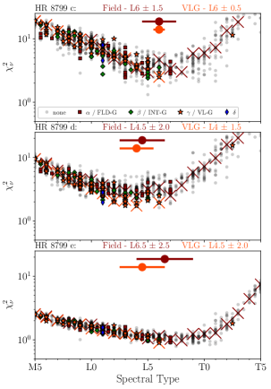
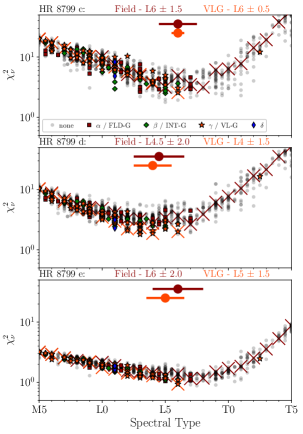
Figure 9: Left: Unrestricted $\chi^{2}$ fit of spectral library objects to the combined H & K GPI spectrum. The unrestricted fit allows the normalization to vary between H and K1+K2 bands. Right: Restricted $\chi^{2}$ fit of spectral library objects to the combined H & K GPI spectrum. The restricted fit only allows the normalization to vary within the uncertainty of photometric calibration. The two agree within error in all cases.

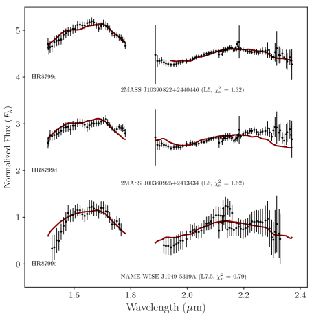
Figure 10: Best fit object to each of HR 8799 c, d, and e spectra within the described spectral library. Both the unrestricted and restricted case fits yielded the same best fitting object spectrum (Zhang et al., 2009; Chiu et al., 2006; Schneider et al., 2014; Luhman, 2013).

Lastly, we show the best fit object spectrum from our spectral library overplotted on the GPI spectra in Figure 10. We show these for both unrestricted and restricted cases. The object names, spectral types, and reduced $\chi^{2}$ are displayed.

In general, each object is best represented by a mid-to-late L-type spectrum. A lack of spectral standards for gravity indicators for late L-types limits the gravity classification based on these fits. The unrestricted and restricted fits generally agree for spectral type. For the unrestricted fit the same object provides the best fit for both c and e.

Planet c is consistent with spectral type $\sim$ L6, both for the individual band fits and the simultaneous fits. The fits to low gravity types indicate earlier spectral type, but likely due to a lack of spectral standards for late L to T-type objects. The H-band spectrum fit, in particular, indicates low gravity (yellow stars). Both unrestricted and restricted fits yield a spectral type L6.0$\pm$1.5 for planet c. The best fit object for both fits is 2MASS J10390822+2440446, which has spectral type L5 (Zhang et al., 2009).

In the case of planet d, the H band spectrum is less peaked. Spectral type $\sim$L4.5 is best fit for both individual bands and simultaneous fits. Again, the H-band fit tends to favor low gravity. The simultaneous fit gives spectral type L4.5$\pm$2.0 for field and L4 $\pm$1.5 for VLG objects, for both the unrestricted and restricted cases. The best fit object in both cases, 2MASS J00360925+2413434, spectral type L6 (Chiu et al., 2006; Schneider et al., 2014).

The individual H and K fits are flatter for e. The H-band and K-band individual fits are consistent with mid-to-late L-type spectrum. The K-band part of the spectrum is consistent with a wide range of spectral types, extending to early T, due in part to large error bars. The simultaneous fit gives spectral type L6.5$\pm$2.5 for the unrestricted fit and L6$\pm$2.0. Both restricted and unrestricted cases yield the best fit for WISE J1049-5319A (Luhman, 2013), classified as type L7.5 Burgasser et al. (2013).

Better wavelength coverage would improve spectral type fitting, as well as a larger library of near-IR spectra and photometry for comparison objects from the field. More low-gravity standards at late spectral types would also also improve the VLG fits. Resolving the discrepancy at the edge of K1 and K2 would also help constrain best fit spectral type for planet e. Variability studies may show additional evidence of cloud holes, a characteristic of objects between L- and T- spectral types Radigan et al. (2014).

5 Comparison to model spectra

We compare our HR 8799 c,d,e spectra with several atmospheric models that have been presented in previous studies to fit the planet spectra and/or photometry. This section is broken up into two sections. The first is a comparison of our spectra to best fit atmospheric models from previous work, A PHOENIX model Barman et al. (2011) that provided the best fit to HR 8799 c in Konopacky et al. (2013), and a set of models from Saumon & Marley (2008), which we refer to as Patchy Cloud models, that provided the best fit for HR 8799 c and d in Ingraham et al. (2014). We compare these to highlight differences between the three spectra and see how well the models hold up to the new data in H-band. The second section compares our spectra to two model grids with varying effective temperature and gravity. The two model grids are the CloudAE-60 model Madhusudhan et al. (2011) and the BT-Settl model Baraffe et al. (2015).

For each set of models, we convolve the model spectrum with a Gaussian to match the spectral resolution of GPI in K-band, and interpolate to the same wavelengths of the GPI spectrum. We adjust the radius so that it minimizes $\chi^{2}$ between the model and our spectra. The models are only matched to our H and K spectra. We also show broadband photometry (Marois et al., 2008, 2010b; Galicher et al., 2011; Currie et al., 2011; Skemer et al., 2012, 2014; Currie et al., 2014; Zurlo et al., 2016), previously compiled in Bonnefoy et al. (2016), leaving out SPHERE H-band points, which are slightly discrepant from our spectra. Table 2 summarizes model parameters fit to each planet. Figure 11 displays each model presented in the table alongside our spectrum and photometry from literature. Each set of models is discussed in detail in the following sections.

Table 2: Best fitting models

Planet	Model	Radius ($M_{Jup}$)	Teff (K)	log(g)	$\log\sigma T_{eff}^{4}4\pi R^{2}/L_{\odot}$
HR 8799 c	PHOENIX (v16)	1.2	1100	3.5	-4.72
	Saumon+ (2008) fixed	1.4	1100	4.0	-4.58
	Saumon+ (2008)	0.8	1300	3.75	-4.78
	Cloud-AE60	0.75	1300	3.5	-4.83
	BT-Settl	0.7	1350	3.5	-4.83
HR 8799 d	PHOENIX (v16)	1.2	1100	3.5	-4.72
	Saumon+ (2008) fixed	1.4	1100	4.0	-4.58
	Saumon+ (2008)	0.8	1300	4.0	-4.78
	Cloud-AE60	0.65	1400	3.5	-4.83
	BT-Settl	0.65	1600	3.5	-4.60
HR 8799 e	PHOENIX (v16)	1.3	1100	3.5	-4.65
	Saumon+ (2008) fixed	1.4	1100	4.0	-4.58
	Saumon+ (2008)	0.9	1300	3.75	-4.68
	Cloud-AE60	1.15	1100	3.5	-4.75
	BT-Settl	0.6	1650	3.5	-4.61

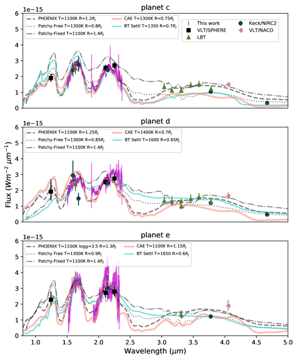
Figure 11: Atmospheric models are plotted in various line styles indicated by the legend for HR 8799 c (top), d (middle), and e (bottom). GPI spectra are plotted as magenta bars. Normalized Phoenix models is displayed with a a thick gray line. For the Saumon & Marley (2008) patchy cloud models, the normalized models are plotted in thin solid blue lines, while the fixed models are plotted in dash-dot lines. Cloud-AE models are plotted as a dotted line, and BT-Settl models as dashed lines. We also plot broadband photometry from previous work, with symbols corresponding to each instrument. Black squares correspond to VLT/SPHERE IRDIS (Zurlo et al., 2016), teal circles to Keck/NIRC2 (Marois et al., 2008, 2010b; Galicher et al., 2011; Currie et al., 2011), green vertical triangles to LBT (Skemer et al., 2012, 2014), and pink left-pointing triangles to NACO (Currie et al., 2014).

5.1 Published Best-Fit Models

5.1.1 PHOENIX model

The PHOENIX (v16) models from Barman et al. (2011) are a set of parameterized models with clouds, where clouds consist of a complex mixture or particles whose state depend on temperature and pressure. This set of models takes into account the transition between cloudless and cloudy atmosphere, as seen between L- and T-type objects. The model is designed to identify the major physical properties of the atmosphere.

Konopacky et al. (2013) presented a best fit model to a Keck/OSIRIS spectrum of HR 8799 c by fitting wavelength ranges and features that were most sensitive to each model parameter (such as gravity, effective temperature, and cloud thickness), checking consistency with broadband photometry. A combination of dynamical stability, age, and interior structure models restricted the fit to $\lesssim 3.5<\mathrm{log}~{}g\lesssim 4.4$ and $900K\lesssim T_{eff}\lesssim 1300K$, leading to a model at $\mathrm{log}~{}g=4.0$ and $T_{eff}=1100K$, moderate cloud thickness, a large eddy diffusion coefficient $K_{zz}=10^{8}cm^{2}s^{-1}$, and super-solar C/O.

We normalize (by scaling the radius) the model to fit each spectrum and show it as the dashed line in Figure 11. We note that this model was fit to a higher resolution spectrum and still provides a good match to both our lower resolution K-band spectrum of c as well as the new H-band spectrum. While the model was fit to the spectrum of HR 8799 c we show it alongside all three spectra for comparison. Based on our comparison in §3.1 (Figure 7) we do not expect it to provide a good fit for d, but could possibly fit e within errorbars. We see that this model does not capture the shape of the K-band spectrum of d nor the flatter H-band spectrum. The model is reasonably consistent with e, within the large errobars. This model, while scaled just to our H & K spectra, is most consistent with the $3-5\mu m$ photometry in all 3 cases. This highlights the importance of obtaining spectra, which will show more detailed differences between objects and can better distinguish between models.

5.1.2 Patchy cloud model (Saumon & Marley, 2008)

Models from Saumon & Marley (2008) are evolution models for brown dwarfs and giant planets in the “hot start” scenario that include patchy clouds. These are parameterized based on effective temperature, cloud properties (cloud hole fraction), gravity, and mixing properties, namely a sedimentation parameter $f_{sed}$ defined in Ackerman & Marley (2001), the ratio between the sedimentation velocity and the convective velocity scale. Ingraham et al. (2014) fit Patchy Cloud models to GPI spectra of c and d, in two cases: first with fixed radius (based on evolutionary models), and then with the radius allowed to vary. The fixed-radius models both had $T_{eff}=1100K$ with thick clouds including some horizontal variation to account for observed J-band flux. The model that provided the best fit for c has $f_{sed}$ of 0.25 and cloud hole fraction of 5% and the best fit for d has $f_{sed}$=0.50 and no holes. The free-radius models both have $T_{eff}=1300K$, but require a radius of $<1R_{Jup}$. The best fit for c has $f_{sed}$=1, without cloud holes and the best fit for d has $f_{sed}=0.5$ and 5% holes.

Ingraham et al. (2014) found that while fixed-radius models are able to reproduce the planet broadband SEDs, they were consistent with the more detailed spectra. We show the described models alongside the spectra of all three planets (Figure 11). The best fitting models for c provided a better fit to HR8799 e and we show this alongside the e spectrum. Similar to Ingraham et al. (2014), we find that the free-radius model provides a better fit to both the H and K band spectra, but not the $3-5\mu m$ photometry, and that while the fixed-radius model fits broadband photometry, it does not provide a good fit to our spectra. For c and d fitting both the H and K spectrum for the best scaling leads to a poorer fit of the K-band portion, and this is especially obvious for the longer wavelength part of d’s K band spectrum. For e, while both models match the peak flux at H and K within the large error bars, they do not capture the band edges. In general, the models do not capture the relative flux between H and K in all cases.

The free-radius models may be missing some effect that leads to requiring sub-$R_{Jup}$ radii to match the observed spectrum. Modeling these objects may require one or a combination of clouds, non-equilibrium chemistry, and non-solar metallicity to be consistent with both the broadband SED and spectroscopy.

5.1.3 A Note on Composition

Konopacky et al. (2013) found margnial evidence for higher C/O ratio for HR8799 c compared to the host star, which has implications on the planet formation history as suggested by Öberg et al. (2011). Without detailed high resolution spectra our results cannot constrain abundances, but it is encouraging that the same model, based on the strongest spectral line indicators also provides a good fit for our lower resolution spectrum and new H-band data. Our data do show evidence of clear differences between the spectra, suggesting there could be differences between the compositions. These differences could also be the result of first order physical effects, rather than composition.

Lavie et al. (2017) attempted to recover abundances of the HR8799 planets through atmospheric retrieval. Given the differences we see in our spectra, including new data, some of the differences seen in Lavie et al. (2017) could be real. We additionally present new K-band data for e, which they conclude is require to estimate C/O and C/H ratios. However the issue of unrealistic radii, as discussed in their study remains to be an unsolved problem of modeling. Until atmospheric models can provide a physically motivated reason for lower observed flux (that often leads to reducing the radius). More spectroscopy, especially at higher resolution, could help identify the dominant effect, whether clouds (e.g., Saumon & Marley, 2008; Burningham et al., 2017), non-equilibrium chemistry (e.g., Barman et al., 2011), composition (e.g., Lee et al., 2013), atmospheric processes (e.g., Tremblin et al., 2017), or some combination. JWST near-IR and mid-IR spectroscopy could help resolve what physical mechanism drives this effect to more accurately determine atmospheric compositions.

5.2 Model grids

5.2.1 CloudAE-60 model grid

We consider the CloudAE-60 model grid (Madhusudhan et al., 2011), also discussed in Bonnefoy et al. (2016). These models represent thick forsterite clouds at solar metallicity with mean particle size of 60$\mu m$. These models do not account for disequilibrium chemistry. We fit the grid of models between 1100 and 1600K and scale to the best fitting radius. In Figure 11 we plot the CloudAE-60 model that minimizes $\chi^{2}$.

This set of models is able to reproduce the K-band spectra of c and e fairly well all the way to band edges. The model does not match the shape of the d spectrum, neither representing the flatter H-band spectrum, nor the rising K-band spectrum. We find similar best fitting effective temperature for e as in Bonnefoy et al. (2016). All three cases produce models that require radii below $1R_{Jup}$. The models that best-fit the H & K spectra do not match the flux at 3-5 $\mu$m.

5.2.2 BT-Settl model grid

Lastly, the BT-Settl 2014 evolutionary model grid for low mass stars couples atmosphere and interior structures (Baraffe et al., 2015). We consider a temperature range from $1200-1700$K and gravity range $\log{g}=3.0-4.0$, encompassing the best fits shown in Bonnefoy et al. (2016). The grid provides models in steps of 100K; to estimate intermediate temperatures, we average models to search in steps 50K. We show these best fit parameters in Figure 11.

We find similar best fitting effective temperatures and gravity as Bonnefoy et al. (2016). This model better reflects the rising slope in K for planet d and in this case is roughly consistent with photometry beyond 3$\mu$m. These models also under-predict flux from 3-5$\mu$m in some cases. Bonnefoy et al. (2016) similarly noted that this model did not match both the Y-H spectra and the 3-5 $\mu$m flux, possibly indicating that it does not produce enough dust at high altitudes. In both studies this model matches the planet d photometry better than for c.

6 Summary and Conclusions

We have implemented a forward modeling approach to recovering IFS spectra from GPI observations of the HR 8799 planets c, d and e. Using this approach we have re-reduced data first presented in Ingraham et al. (2014) as well as new H-band data with this new algorithm, finding as in Pueyo (2016) that algorithm parameters converge with increasing $k_{klip}$. With this approach we are able to recover a K-band spectrum on HR 8799 e for the first time. While the HR 8799 planet SEDs have been typically shown to be very similar, their more detailed spectra show evidence of different atmospheric properties. In addition to showing that there is statistical difference between c and d, different atmospheric models also provide best fits to each spectrum. These differences could be the result of properties such as cloud fraction, non-equilibrium chemistry, composition, and/or thermal structure. We have shown that a range of models with difference physical mechanisms can provide similar fits to our H & K spectra.

While the large errorbars of HR 8799 e make it hard to determine its similarity to the other two planet spectra, but we find that c and d are distinct. The dominant effect comes from the relative flux between H and K bands; the differences go away when we normalize the spectra in each band individually (see Appendix C). With less noisy K-band data we could make a stronger statement about difference between these and planet e. It is likely the K-band spectrum for e resembles that of d and that our K1 band edge is biased by residual speckle noise. Given the mid-late L-spectral types of all three planets, they may display variability. Planet e could be a good candidate for variability study, since it appears to have a brighter H-band spectrum, suggestive of cloud holes in transition from L-T (e.g., Radigan et al., 2014).

The following summarize the main points of our results:

• The KLIP-FM method is able to recover a spectrum of close-in planet e, despite many residual speckles. By exploring results over varying $k_{klip}$ and $mov$ we the relatively low dependence of our result on algorithm parameters. This is especially true for the H-band data, which had greater field rotation.

• Our H spectra of planets d and e are consistent at the short end with YJH spectra from the SPHERE/VLT instrument (Zurlo et al., 2016).

• The H & K spectrum of HR 8799 c is statistically different ($>5\sigma$) from d based on our $\chi^{2}_{i,j}$ measurement.

• All three objects are best matched by mid to late L-type field brown dwarfs from a library of near-infrared spectra. Evidence of L-T transition variability could support models with inhomogeneous cloud coverage.

• The PHOENIX model, which was fit to higher resolution K-band spectroscopy of HR 8799 c also fits both our lower resolution H and K-band spectra, as well as 3-5 $\mu$m, without requiring sub-$M_{Jup}$ radii. We have compared it to the spectra of d and e as a reminder that even if the broadband photometry is similar, the same model will not provide a good fit for all objects in the system.

• A general grid of models is not expected to provide the same level of detailed fit as a detailed study, however the CloudAE models produce very similar results for our H-K spectra as the PHOENIX model, while invoking different mechanisms. The BT-Settl models seem to represent the H & K spectra of d best, while also matching $3-5\mu m$ photometry. The model grids also require sub-$M_{Jup}$ radii in most cases.

Spectroscopic information is necessary for revealing compositional differences between the HR 8799 planets. However, more work is needed to accurately measure abundances. That most models require unreasonable radii indicate that they are missing a physical mechanism to fully account for the observed flux, similarly discussed in many previous studies as an “under-luminosity problem” that indicates a discrepancy between atmospheric models and evolutionary models (e.g., Marois et al., 2008; Bowler et al., 2010; Marley et al., 2012). While this problem could be accounted for by a prescription of clouds (e.g., Madhusudhan et al., 2011), chemistry (e.g., Barman et al., 2011), or thermal structure (e.g., Tremblin et al., 2017), the true process is not solved. When the correct physical mechanism is understood, modeling and/or atmosphere retrievals should be able to measure abundances accurately. Larger spectral coverage could help distinguish between different processes. Higher spectroscopic resolution would provide more detail to probe atmospheric chemistry, which could be achieved with next generation Extremely Large Telescopes (ELTs) that combine high resolution spectroscopy with high contrast imaging (as described in Snellen et al., 2015).

JWST will be able to deliver spectra at longer wavelengths for better characterization planetary mass companions at 3-5$\mu$m and beyond. Given the reduced inner working angle and limited rotation compared to ground-based 8m-class telescopes, forward modeling may be important for obtaining infrared companion spectra to systems like HR 8799, helping to advance atmospheric modeling efforts and provide benchmark objects for future high contrast imaging studies.

Appendix A Residuals

After optimizing KLIP parameters, described in section 2.2, we display the PSF-subtracted data stamp that contains the planet and the forward model, summed over the bandpass, and the residual between the two (Figure 12). We show the residual plots for all three planets in each H, K1, and K2 bands, summed over the wavelength axis.

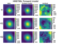
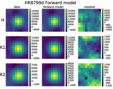
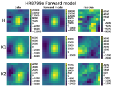
Figure 12: A summary of the forward model performance for HR 8799 c (left) d (middle) and e (right). Klipped data is shown to the left, the forward model is in the middle panel and the rightmost panel shows the difference between these two. Each image stamp is summed over the bandpass. Pixel values are in raw data units. Residual speckle noise appears to be influencing the K1 reduction of HR 8799 e.

Increased speckle noise close to the focal plane mask of the image contributes larger residuals for the forward model of HR 8799 e. However, as can be seen in the Figure 12, the forward model captures the self-subtraction negative lobes. We have taken care to remove obvious contaminants, including a bad pixel in several wavelength channels near HR 8799 d.

Appendix B Comparing algorithms

We compare our spectral extraction with the reductions from two other algorithms. We expect KLIP-FM to perform well especially at small inner working angle and when the companion is faint. The recovery of the more widely separated c and d planets provide a good validation of the forward modeling algorithm. Some flux loss is expected when the forward model assumptions are not completely appropriate, as described in Pueyo (2016) and as we have discussed in §2.2.

The two PSF subtraction pipelines we compare with were both used for the discovery of 51 Eri b and are fully described in Macintosh et al. (2015). These use the cADI and TLOCI algorithms, respectively. We show results from the three pipelines together in Figure 13. We briefly recall the important steps for each pipeline, which starts from the same calibrated datacubes generated by the Data Cruncher (Wang et al., 2018), and perform the PSF subtraction and signal extraction.

In the first pipeline the images are high-pass filtered with an apodized Fourier-space filter following a Hanning profile. The filtering is done early in the process to simultaneously affect both satellite spots and planets. We tested different cutoff frequencies were tested. We found planet c to be particularly sensitive the size of the filter in the K band datasets. Being brighter than the spot in a speckle-free region of the image, its absolute flux was hard to calibrate based on the residuals after forward-modeling through inserting simulated signals. The best results were found with a cutoff frequency of 8 equivalent-pixels in the image plane for planets c and d. For planet e which is heavily embedded in the speckle field, a more agressive filter with a cutoff frequency of 4 equivalent-pixels was applied. At each wavelength, a model of the PSF for the forward model was built from the average of the four spots in each image, further combined along the time dimension. The PSF subtraction was applied with the cADI algorithm (Marois et al., 2006a; Lagrange et al., 2010). To accurately measure the position of each planet, the residuals were stacked along the spectral dimension. The position was extracted with an amoeba algorithm that minimizes the squared residuals, after subtracting the forward-model to the planet’signal, in a $2\times 2$ FWHM wedge centered on the planet. The spectrum of each planet was then extracted with the same technique but fixing the position of the forward model at the best fitted position. Uncertainties were estimated from the dispersion of the recovered signal of fake sources that were injected at the same separation but twenty different position angles uniformly distribution between $90$ and $270^{\circ}$ apart from each planet.

The second pipeline uses the TLOCI algorithm, which combines both SDI and ADI data into one stellar subtraction step. Generic methane/dusty input spectra were used to guide the reference image selection process to minimize self-subtraction and maximize the signal-to-noise for any companion with a spectrum similar to the input spectra. A maximum flux contamination ratio of 90% inside a 1.5 $\lambda/D$ aperture was chosen for this analysis. The algorithm uses a pixel mask to avoid fitting the planet flux with the algorithm and an 11x11 pixel (3x3 $\lambda/D$) median high-pass filter. Circular annulus subtraction regions have 1.7 $\lambda/D$ width. The least-squares optimization regions are also circular annuli just inside and outside the subtraction regions, having 3 $\lambda/D$ width for the inner annulus and 6.6 $\lambda/D$ width for the outer annulus. To determine the companion spectrum, a polychromatic forward model is generated from the least-squares coefficients and the stellar PSF (obtained from median averaging the four off-axis calibration spots) mimicking the exoplanet signal, including the negative “wings” from self-subtraction. This model is adjusted in position (sub-pixel accuracy) and flux using an iterative technique that minimizes the residual local noise in an aperture after subtracting the forward model from the exoplanet candidate signal. Photometric error bars are estimated at each wavelength by taking the standard deviation of the same extraction process performed on simulated exoplanets (using the same polychromatic forward model) located at the exoplanet candidate separation, but at different position angles.

Overall, the KLIP-FM spectra match the cADI and/or TLOCI spectra in most cases as shown in Figure 13. The KLIP forward modeling algorithm and the cADI-based pipeline show excellent agreement for planet d, for planet c at H band, and at the $\lesssim 1\sigma$ level for planet e. The cADI pipeline is $1\sigma$ brighter at K band. This discrepancy is likely due to the impact of different high-pass filters as discussed before. The TLOCI and KLIP-FM pipelines show the same excellent agreement for planet c and is slightly fainter for planet d towards the end of H band. The TLOCI analysis agrees with KLIP-FM within the large errorbars for planet e.

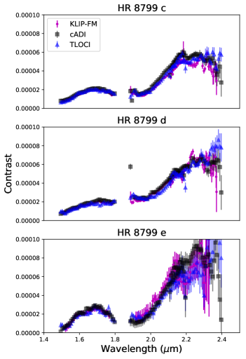
Figure 13: Comparison of the KLIP forward modeling algorithm reduction presented in this paper (magenta circles) with cADI (black squares) and TLOCI (blue triangles) reductions. The planet-to-star contrast is plotted vs. wavelength.

Appendix C Spectrum comparison by band

We show the individual spectra comparisons between HR 8799 c, d, and e as described in Equation 7. Here we normalize the spectrum in each band, rather than over the entire H-K range. Figures 14-16 show the individual comparison for each band.

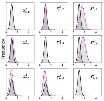
Figure 14: Comparison of $\chi^{2}$ distributions for H band.

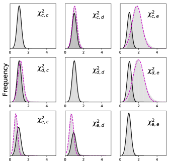
Figure 15: Comparison of $\chi^{2}$ distributions for K1 band.

The overall shapes of the spectra within each band are not very different within errorbars. Figures 14-16 show considerable overlap in the distributions. However, the relative flux between H and K bands for the three planets is an obvious difference between them (which also drives the atmospheric model fitting) that is not captured by the individual band comparison of low resolution spectra.

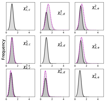
Figure 16: Comparison of $\chi^{2}$ distributions for K2 band.

Appendix D Full reduced spectrum

We provide our $1.5-2.4\mu m$ reduced spectrum in Table 3.

Table 3: GPI spectrum of the HR 8799 c, d, and e in flux units at 10pc.

c: $\lambda$	Flux	Error	d: $\lambda$	Flux	Error	e: $\lambda$	Flux	Error
($\mu m$)	($Wm^{-2}\mu m^{-1}$)	($Wm^{-2}\mu m^{-1}$)	($\mu m$)	($Wm^{-2}\mu m^{-1}$)	($Wm^{-2}\mu m^{-1}$)	($\mu m$)	($Wm^{-2}\mu m^{-1}$)	($Wm^{-2}\mu m^{-1}$)
1.50776	1.73145E-15	2.79261E-16	1.50776	1.33467E-15	2.88152E-16	1.50776
1.51072	1.46075E-15	2.55719E-16	1.51072	1.44751E-15	2.50840E-16	1.51072
1.51495	1.56397E-15	2.62620E-16	1.51495	1.88622E-15	2.62037E-16	1.51495
1.52168	1.59637E-15	2.71240E-16	1.52168	1.85274E-15	2.54648E-16	1.52168	1.00613E-15	8.32404E-16
1.52962	1.82500E-15	2.63159E-16	1.52962	1.88055E-15	2.59543E-16	1.52962	1.10141E-15	7.53412E-16
1.53807	1.89682E-15	2.51584E-16	1.53807	1.98775E-15	2.54490E-16	1.53807	1.62327E-15	7.52152E-16
1.54601	1.92735E-15	2.43479E-16	1.54601	2.09302E-15	2.44374E-16	1.54601	1.74446E-15	5.72797E-16
1.55387	1.95888E-15	2.23333E-16	1.55387	2.13862E-15	2.31782E-16	1.55387	2.44538E-15	4.77751E-16
1.56234	2.20817E-15	2.26991E-16	1.56234	2.30514E-15	2.45245E-16	1.56234	2.64150E-15	5.18419E-16
1.57074	2.28764E-15	2.15666E-16	1.57074	2.33754E-15	2.43456E-16	1.57074	2.75700E-15	5.71800E-16
1.57898	2.38194E-15	2.07432E-16	1.57898	2.36517E-15	2.49826E-16	1.57898	3.37050E-15	4.86809E-16
1.58728	2.39028E-15	1.98210E-16	1.58728	2.22597E-15	2.46330E-16	1.58728	3.20412E-15	3.65439E-16
1.5957	2.50643E-15	2.04841E-16	1.5957	2.49010E-15	2.51572E-16	1.5957	3.23819E-15	4.05298E-16
1.60374	2.51859E-15	1.83617E-16	1.60374	2.49566E-15	2.07153E-16	1.60374	3.50249E-15	4.09458E-16
1.61209	2.71523E-15	1.96294E-16	1.61209	2.68137E-15	2.17858E-16	1.61209	3.64782E-15	3.79600E-16
1.62078	2.73097E-15	1.89629E-16	1.62078	2.71290E-15	1.90383E-16	1.62078	3.53528E-15	3.34049E-16
1.62895	2.69177E-15	1.70791E-16	1.62895	2.64639E-15	2.09287E-16	1.62895	3.24040E-15	3.56117E-16
1.63718	2.68906E-15	1.63056E-16	1.63718	2.56599E-15	2.12826E-16	1.63718	3.11055E-15	3.63156E-16
1.646	2.81385E-15	1.64888E-16	1.646	2.40662E-15	2.29716E-16	1.646	3.31398E-15	3.81471E-16
1.65415	2.85857E-15	1.68992E-16	1.65415	2.52209E-15	2.42221E-16	1.65415	3.69580E-15	4.54456E-16
1.66191	2.91661E-15	1.68455E-16	1.66191	2.62517E-15	2.04352E-16	1.66191	3.61348E-15	4.12620E-16
1.6697	2.84368E-15	1.57134E-16	1.6697	2.62696E-15	1.72916E-16	1.6697	3.52549E-15	4.24976E-16
1.67826	2.69356E-15	1.50773E-16	1.67826	2.61324E-15	1.59223E-16	1.67826	3.45127E-15	3.69226E-16
1.68659	2.53747E-15	1.58609E-16	1.68659	2.62474E-15	1.52072E-16	1.68659	3.29716E-15	3.95526E-16
1.69548	2.67212E-15	1.58928E-16	1.69548	2.74329E-15	1.60122E-16	1.69548	3.59782E-15	3.86855E-16
1.70379	2.79548E-15	1.75119E-16	1.70379	2.81561E-15	1.83871E-16	1.70379	3.62358E-15	3.96528E-16
1.71256	2.68000E-15	1.91466E-16	1.71256	2.84797E-15	1.91948E-16	1.71256	3.38168E-15	4.28278E-16
1.71826	2.63503E-15	1.72197E-16	1.71826	2.61451E-15	1.78198E-16	1.71826	3.30321E-15	3.66134E-16
1.72562	2.49994E-15	1.58232E-16	1.72562	2.47666E-15	1.46859E-16	1.72562	2.80979E-15	3.23274E-16
1.73395	2.27136E-15	1.38421E-16	1.73395	2.34448E-15	1.37585E-16	1.73395	2.34737E-15	3.33969E-16
1.74305	2.16220E-15	1.25966E-16	1.74305	2.19943E-15	1.25607E-16	1.74305	2.43047E-15	3.08768E-16
1.75139	2.18413E-15	1.55635E-16	1.75139	2.32768E-15	1.39663E-16	1.75139	2.64743E-15	3.34755E-16
1.75923	2.09152E-15	1.57566E-16	1.75923	2.48106E-15	1.42337E-16	1.75923	2.37151E-15	3.60365E-16
1.76602	2.03956E-15	1.51567E-16	1.76602	2.38054E-15	1.52851E-16	1.76602	1.94834E-15	3.88357E-16
1.77172	1.93018E-15	1.43464E-16	1.77172	2.33128E-15	1.92200E-16	1.77172
1.77686	1.85298E-15	1.41944E-16	1.77686	2.21941E-15	2.01857E-16	1.77686
1.78121	1.63147E-15	1.37720E-16	1.78121	2.07282E-15	2.04131E-16	1.78121
1.88723	2.03801E-15	1.36498E-15	1.88723	2.30577E-15	1.44160E-15	1.88723
1.89436	1.47770E-15	2.71668E-16	1.89436	1.88868E-15	2.94845E-16	1.89436
1.90174	1.47124E-15	1.43759E-16	1.90174	1.88607E-15	2.12447E-16	1.90174
1.9096	1.54153E-15	1.45717E-16	1.9096	2.09433E-15	1.66364E-16	1.9096
1.91714	1.34378E-15	1.39897E-16	1.91714	1.99324E-15	1.44480E-16	1.91714	2.31105E-15	5.16806E-16
1.92461	1.25976E-15	1.27087E-16	1.92461	1.99658E-15	1.48204E-16	1.92461	2.09120E-15	5.32716E-16
1.93272	1.18958E-15	1.16669E-16	1.93272	1.92186E-15	1.37709E-16	1.93272	1.99156E-15	5.68846E-16
1.94265	1.12703E-15	9.82724E-17	1.94265	1.76872E-15	1.17088E-16	1.94265	1.89713E-15	5.07610E-16
1.95281	1.13187E-15	1.13328E-16	1.95281	1.83061E-15	1.36893E-16	1.95281	1.96871E-15	5.13199E-16
1.96161	1.17873E-15	1.13429E-16	1.96161	1.86198E-15	1.39680E-16	1.96161	1.96727E-15	5.34209E-16
1.96938	1.28330E-15	1.08946E-16	1.96938	1.84856E-15	1.22501E-16	1.96938	1.96955E-15	5.17002E-16
1.97667	1.32508E-15	1.04380E-16	1.97667	1.78353E-15	1.10631E-16	1.97667	2.11890E-15	5.43009E-16
1.98473	1.41538E-15	1.07500E-16	1.98473	1.88182E-15	1.28567E-16	1.98473	2.18175E-15	5.51286E-16
1.99717	1.44730E-15	1.07762E-16	1.99717	2.06136E-15	1.54830E-16	1.99717	2.30878E-15	5.05001E-16
2.0109	1.57343E-15	9.40893E-17	2.0109	2.17861E-15	1.47850E-16	2.0109	3.04514E-15	4.85159E-16
2.01902	1.66693E-15	9.81417E-17	2.01902	2.16205E-15	1.27782E-16	2.01902	2.88466E-15	3.57436E-16
2.02545	1.74980E-15	1.12876E-16	2.02545	2.13171E-15	1.25974E-16	2.02545	2.90724E-15	3.86474E-16
2.03165	1.82837E-15	1.06535E-16	2.03165	2.08902E-15	1.16510E-16	2.03165	2.72256E-15	3.74589E-16
2.0406	1.91342E-15	9.31512E-17	2.0406	2.17134E-15	1.19445E-16	2.0406	2.69971E-15	4.04758E-16
2.04977	1.96417E-15	8.96671E-17	2.04977	2.32241E-15	1.05412E-16	2.04977	2.76381E-15	4.49176E-16
2.05939	2.06224E-15	9.14667E-17	2.05939	2.34754E-15	9.66011E-17	2.05939	3.04182E-15	4.10525E-16
2.06838	2.14385E-15	1.00008E-16	2.06838	2.45222E-15	1.06841E-16	2.06838	3.27945E-15	4.08582E-16
2.07634	2.18938E-15	9.48017E-17	2.07634	2.56451E-15	1.11055E-16	2.07634	3.31831E-15	4.36232E-16
2.08445	2.24628E-15	8.64849E-17	2.08445	2.65357E-15	1.06652E-16	2.08445	3.43399E-15	4.81935E-16
2.09321	2.31436E-15	9.27182E-17	2.09321	2.68320E-15	1.11878E-16	2.09321	3.74805E-15	5.26672E-16
2.10191	2.39196E-15	9.73509E-17	2.10191	2.72654E-15	1.09539E-16	2.10191	3.96360E-15	5.41321E-16
2.11049	2.39048E-15	8.39771E-17	2.11049	2.71716E-15	9.62034E-17	2.11049	3.97294E-15	5.21006E-16
2.11872	2.41553E-15	8.06201E-17	2.11872	2.72546E-15	1.04323E-16	2.11872	3.87817E-15	5.07542E-16
2.12672	2.51533E-15	8.24227E-17	2.12672	2.86541E-15	1.20287E-16	2.12672	4.43579E-15	5.32689E-16
2.13543	2.58310E-15	7.96663E-17	2.13543	2.92595E-15	1.16728E-16	2.13543	4.61147E-15	5.54098E-16
2.1436	2.64299E-15	8.49349E-17	2.1436	2.93367E-15	1.19210E-16	2.1436	4.56206E-15	4.76897E-16
2.15136	2.69969E-15	1.04414E-16	2.15136	2.89564E-15	1.35568E-16	2.15136	4.37690E-15	4.72580E-16
2.15869	2.65026E-15	7.99967E-17	2.15869	2.71841E-15	1.10909E-16	2.15869	4.10472E-15	4.84592E-16
2.16564	2.44528E-15	7.95661E-17	2.16564	2.46122E-15	1.15686E-16	2.16564
2.17139	2.67017E-15	7.95072E-17	2.17139	2.53147E-15	1.59061E-16	2.17139
2.17686	3.02815E-15	1.27952E-16	2.17686	2.50246E-15	2.02441E-16	2.17686
2.18372	3.20672E-15	7.57003E-16	2.18372	2.92986E-15	7.19543E-16	2.18372
2.11263	2.08220E-15	1.76446E-16	2.11263	2.05871E-15	2.52649E-16	2.11263
2.12373	2.09741E-15	9.77512E-17	2.12373	2.26295E-15	1.73276E-16	2.12373
2.12933	2.46793E-15	1.23434E-16	2.12933	2.63819E-15	1.51924E-16	2.12933
2.13518	2.44913E-15	1.06935E-16	2.13518	2.67962E-15	1.36449E-16	2.13518	3.86352E-15	5.79448E-16
2.14195	2.47287E-15	1.17533E-16	2.14195	2.69382E-15	1.26388E-16	2.14195	3.17669E-15	6.01422E-16
2.14931	2.65851E-15	1.09262E-16	2.14931	2.81641E-15	1.18280E-16	2.14931	3.28187E-15	5.88484E-16
2.15691	2.68898E-15	1.11227E-16	2.15691	2.71622E-15	1.15086E-16	2.15691	2.95467E-15	4.96899E-16
2.16488	2.42844E-15	9.81085E-17	2.16488	2.48631E-15	1.16156E-16	2.16488	2.78672E-15	4.37103E-16
2.17325	2.49722E-15	9.83552E-17	2.17325	2.72076E-15	1.14770E-16	2.17325	2.80869E-15	5.21278E-16
2.18182	2.65795E-15	9.98303E-17	2.18182	2.99062E-15	1.08101E-16	2.18182	2.80975E-15	6.80945E-16
2.18959	2.58605E-15	9.58642E-17	2.18959	2.88759E-15	1.08781E-16	2.18959	2.74018E-15	6.93414E-16
2.19772	2.50921E-15	8.67402E-17	2.19772	3.05906E-15	1.20869E-16	2.19772	2.71717E-15	6.90955E-16
2.20595	2.42639E-15	7.93267E-17	2.20595	3.17959E-15	1.37906E-16	2.20595	2.74455E-15	6.83315E-16
2.21398	2.33961E-15	1.05765E-16	2.21398	3.06283E-15	1.45510E-16	2.21398	3.01822E-15	6.40675E-16
2.22188	2.33618E-15	1.15906E-16	2.22188	3.19849E-15	1.46380E-16	2.22188	3.19992E-15	6.88742E-16
2.22866	2.28167E-15	9.73196E-17	2.22866	3.20375E-15	1.49208E-16	2.22866	3.47627E-15	7.44844E-16
2.23696	2.28333E-15	1.26116E-16	2.23696	3.24555E-15	1.37603E-16	2.23696	3.52536E-15	7.94122E-16
2.24522	2.29734E-15	1.27417E-16	2.24522	3.01478E-15	1.57085E-16	2.24522	3.63362E-15	7.75792E-16
2.2519	2.21698E-15	1.05537E-16	2.2519	2.82656E-15	1.58374E-16	2.2519	3.47115E-15	7.63492E-16
2.25911	2.35405E-15	1.34450E-16	2.25911	3.07052E-15	1.62839E-16	2.25911	3.60626E-15	7.87863E-16
2.26625	2.38989E-15	1.57034E-16	2.26625	3.12404E-15	1.67920E-16	2.26625	3.47341E-15	8.93141E-16
2.2761	2.40367E-15	1.71859E-16	2.2761	3.07075E-15	2.27538E-16	2.2761	3.83657E-15	1.00173E-15
2.28424	2.47536E-15	3.60119E-16	2.28424	3.28311E-15	3.82843E-16	2.28424	4.12671E-15	1.25140E-15
2.29125	2.14047E-15	1.97341E-16	2.29125	2.91484E-15	2.28448E-16	2.29125	3.06066E-15	1.27180E-15
2.29894	1.82729E-15	1.39034E-16	2.29894	2.54871E-15	2.13205E-16	2.29894	2.10342E-15	1.29480E-15
2.30465	1.83450E-15	1.18788E-16	2.30465	3.00497E-15	2.56827E-16	2.30465	2.05041E-15	1.44621E-15
2.31086	2.28488E-15	4.34866E-16	2.31086	3.18844E-15	4.97568E-16	2.31086	2.90437E-15	1.75422E-15
2.31651	2.63187E-15	7.94890E-16	2.31651	3.11156E-15	8.20462E-16	2.31651	3.33332E-15	2.22156E-15
2.32505	2.02439E-15	3.89874E-16	2.32505	2.75737E-15	4.14954E-16	2.32505	2.57146E-15	1.72444E-15
2.32872	1.97924E-15	3.45239E-16	2.32872	2.94873E-15	3.64429E-16	2.32872	1.90773E-15	1.80550E-15
2.33642	2.15101E-15	2.19251E-16	2.33642	2.39595E-15	2.87636E-16	2.33642
2.34302	1.80835E-15	1.82389E-16	2.34302	2.08174E-15	3.85605E-16	2.34302
2.35053	1.64353E-15	4.29150E-16	2.35053	2.58858E-15	5.47837E-16	2.35053
2.35321	1.43145E-15	3.85427E-16	2.35321	2.88627E-15	5.00554E-16	2.35321
2.36288	1.80437E-15	3.47187E-16	2.36288	3.09159E-15	4.73127E-16	2.36288
2.36766	1.50262E-15	4.21286E-16	2.36766	2.59120E-15	5.11897E-16	2.36766
2.36972	1.16197E-15	6.98525E-16	2.36972	2.02990E-15	9.53985E-16	2.36972

References

- Ackerman & Marley (2001) Ackerman, A. S., & Marley, M. S. 2001, ApJ, 556, 872, doi: 10.1086/321540
- Allers & Liu (2013) Allers, K. N., & Liu, M. C. 2013, ApJ, 772, 79, doi: 10.1088/0004-637X/772/2/79
- Apai et al. (2016) Apai, D., Kasper, M., Skemer, A., et al. 2016, ApJ, 820, 40, doi: 10.3847/0004-637X/820/1/40
- Astropy Collaboration et al. (2013) Astropy Collaboration, Robitaille, T. P., Tollerud, E. J., et al. 2013, A&A, 558, A33, doi: 10.1051/0004-6361/201322068
- Baines et al. (2012) Baines, E. K., White, R. J., Huber, D., et al. 2012, ApJ, 761, 57, doi: 10.1088/0004-637X/761/1/57
- Baraffe et al. (2015) Baraffe, I., Homeier, D., Allard, F., & Chabrier, G. 2015, A&A, 577, A42, doi: 10.1051/0004-6361/201425481
- Barman et al. (2015) Barman, T. S., Konopacky, Q. M., Macintosh, B., & Marois, C. 2015, ApJ, 804, 61, doi: 10.1088/0004-637X/804/1/61
- Barman et al. (2011) Barman, T. S., Macintosh, B., Konopacky, Q. M., & Marois, C. 2011, ApJ, 733, 65, doi: 10.1088/0004-637X/733/1/65
- Bonnefoy et al. (2016) Bonnefoy, M., Zurlo, A., Baudino, J. L., et al. 2016, A&A, 587, A58, doi: 10.1051/0004-6361/201526906
- Bowler et al. (2010) Bowler, B. P., Liu, M. C., Dupuy, T. J., & Cushing, M. C. 2010, ApJ, 723, 850, doi: 10.1088/0004-637X/723/1/850
- Burgasser (2014) Burgasser, A. J. 2014, in Astronomical Society of India Conference Series, Vol. 11, Astronomical Society of India Conference Series
- Burgasser et al. (2013) Burgasser, A. J., Sheppard, S. S., & Luhman, K. L. 2013, ApJ, 772, 129, doi: 10.1088/0004-637X/772/2/129
- Burningham et al. (2017) Burningham, B., Marley, M. S., Line, M. R., et al. 2017, MNRAS, 470, 1177, doi: 10.1093/mnras/stx1246
- Chilcote et al. (2017) Chilcote, J., Pueyo, L., De Rosa, R. J., et al. 2017, AJ, 153, 182, doi: 10.3847/1538-3881/aa63e9
- Chiu et al. (2006) Chiu, K., Fan, X., Leggett, S. K., et al. 2006, AJ, 131, 2722, doi: 10.1086/501431
- Cruz et al. (2009) Cruz, K. L., Kirkpatrick, J. D., & Burgasser, A. J. 2009, AJ, 137, 3345, doi: 10.1088/0004-6256/137/2/3345
- Currie et al. (2011) Currie, T., Burrows, A., Itoh, Y., et al. 2011, ApJ, 729, 128, doi: 10.1088/0004-637X/729/2/128
- Currie et al. (2014) Currie, T., Burrows, A., Girard, J. H., et al. 2014, ApJ, 795, 133, doi: 10.1088/0004-637X/795/2/133
- Cushing et al. (2005) Cushing, M. C., Rayner, J. T., & Vacca, W. D. 2005, ApJ, 623, 1115, doi: 10.1086/428040
- De Rosa et al. (2016) De Rosa, R. J., Rameau, J., Patience, J., et al. 2016, ApJ, 824, 121, doi: 10.3847/0004-637X/824/2/121
- Fabrycky & Murray-Clay (2010) Fabrycky, D. C., & Murray-Clay, R. A. 2010, ApJ, 710, 1408, doi: 10.1088/0004-637X/710/2/1408
- Gagné et al. (2015) Gagné, J., Faherty, J. K., Cruz, K. L., et al. 2015, ApJS, 219, 33, doi: 10.1088/0067-0049/219/2/33
- Galicher et al. (2011) Galicher, R., Marois, C., Macintosh, B., Barman, T., & Konopacky, Q. 2011, ApJ, 739, L41, doi: 10.1088/2041-8205/739/2/L41
- Gerard & Marois (2016) Gerard, B. L., & Marois, C. 2016, in Proc. SPIE, Vol. 9909, Adaptive Optics Systems V, 990958
- GPI instrument Collaboration (2014) GPI instrument Collaboration. 2014, GPI Pipeline: Gemini Planet Imager Data Pipeline, Astrophysics Source Code Library. http://ascl.net/1411.018
- Gray & Kaye (1999) Gray, R. O., & Kaye, A. B. 1999, AJ, 118, 2993, doi: 10.1086/301134
- Greco & Brandt (2016) Greco, J. P., & Brandt, T. D. 2016, ApJ, 833, 134, doi: 10.3847/1538-4357/833/2/134
- Hinz et al. (2010) Hinz, P. M., Rodigas, T. J., Kenworthy, M. A., et al. 2010, ApJ, 716, 417, doi: 10.1088/0004-637X/716/1/417
- Hunter (2007) Hunter, J. D. 2007, Computing in Science and Engineering, 9, 90, doi: 10.1109/MCSE.2007.55
- Ingraham et al. (2014) Ingraham, P., Marley, M. S., Saumon, D., et al. 2014, ApJ, 794, L15, doi: 10.1088/2041-8205/794/1/L15
- Janson et al. (2010) Janson, M., Bergfors, C., Goto, M., Brandner, W., & Lafrenière, D. 2010, ApJ, 710, L35, doi: 10.1088/2041-8205/710/1/L35
- Kirkpatrick (2005) Kirkpatrick, J. D. 2005, ARA&A, 43, 195, doi: 10.1146/annurev.astro.42.053102.134017
- Kirkpatrick et al. (2006) Kirkpatrick, J. D., Barman, T. S., Burgasser, A. J., et al. 2006, ApJ, 639, 1120, doi: 10.1086/499622
- Kirkpatrick et al. (2010) Kirkpatrick, J. D., Looper, D. L., Burgasser, A. J., et al. 2010, ApJS, 190, 100, doi: 10.1088/0067-0049/190/1/100
- Konopacky et al. (2013) Konopacky, Q. M., Barman, T. S., Macintosh, B. A., & Marois, C. 2013, Science, 339, 1398, doi: 10.1126/science.1232003
- Konopacky et al. (2016) Konopacky, Q. M., Marois, C., Macintosh, B. A., et al. 2016, AJ, 152, 28, doi: 10.3847/0004-6256/152/2/28
- Konopacky et al. (2014) Konopacky, Q. M., Thomas, S. J., Macintosh, B. A., et al. 2014, in Proc. SPIE, Vol. 9147, Ground-based and Airborne Instrumentation for Astronomy V, 914784
- Lafrenière et al. (2009) Lafrenière, D., Marois, C., Doyon, R., & Barman, T. 2009, ApJ, 694, L148, doi: 10.1088/0004-637X/694/2/L148
- Lagrange et al. (2010) Lagrange, A.-M., Bonnefoy, M., Chauvin, G., et al. 2010, Science, 329, 57, doi: 10.1126/science.1187187
- Lavie et al. (2017) Lavie, B., Mendonça, J. M., Mordasini, C., et al. 2017, AJ, 154, 91, doi: 10.3847/1538-3881/aa7ed8
- Lee et al. (2013) Lee, J.-M., Heng, K., & Irwin, P. G. J. 2013, ApJ, 778, 97, doi: 10.1088/0004-637X/778/2/97
- Luhman (2013) Luhman, K. L. 2013, ApJ, 767, L1, doi: 10.1088/2041-8205/767/1/L1
- Macintosh et al. (2014) Macintosh, B., Graham, J. R., Ingraham, P., et al. 2014, Proceedings of the National Academy of Science, 111, 12661, doi: 10.1073/pnas.1304215111
- Macintosh et al. (2015) Macintosh, B., Graham, J. R., Barman, T., et al. 2015, Science, 350, 64, doi: 10.1126/science.aac5891
- Madhusudhan et al. (2011) Madhusudhan, N., Burrows, A., & Currie, T. 2011, ApJ, 737, 34, doi: 10.1088/0004-637X/737/1/34
- Maire et al. (2014) Maire, J., Ingraham, P. J., De Rosa, R. J., et al. 2014, in Proc. SPIE, Vol. 9147, Ground-based and Airborne Instrumentation for Astronomy V, 914785
- Malo et al. (2013) Malo, L., Doyon, R., Lafrenière, D., et al. 2013, ApJ, 762, 88, doi: 10.1088/0004-637X/762/2/88
- Marley et al. (2012) Marley, M. S., Saumon, D., Cushing, M., et al. 2012, ApJ, 754, 135, doi: 10.1088/0004-637X/754/2/135
- Marois et al. (2014) Marois, C., Correia, C., Galicher, R., et al. 2014, in Proc. SPIE, Vol. 9148, Adaptive Optics Systems IV, 91480U
- Marois et al. (2006a) Marois, C., Lafrenière, D., Doyon, R., Macintosh, B., & Nadeau, D. 2006a, ApJ, 641, 556, doi: 10.1086/500401
- Marois et al. (2006b) Marois, C., Lafrenière, D., Macintosh, B., & Doyon, R. 2006b, ApJ, 647, 612, doi: 10.1086/505191
- Marois et al. (2008) Marois, C., Macintosh, B., Barman, T., et al. 2008, Science, 322, 1348, doi: 10.1126/science.1166585
- Marois et al. (2010a) Marois, C., Macintosh, B., & Véran, J.-P. 2010a, in Proc. SPIE, Vol. 7736, Adaptive Optics Systems II, 77361J
- Marois et al. (2006c) Marois, C., Phillion, D. W., & Macintosh, B. 2006c, in Proc. SPIE, Vol. 6269, Society of Photo-Optical Instrumentation Engineers (SPIE) Conference Series, 62693M
- Marois et al. (2010b) Marois, C., Zuckerman, B., Konopacky, Q. M., Macintosh, B., & Barman, T. 2010b, Nature, 468, 1080, doi: 10.1038/nature09684
- Moór et al. (2006) Moór, A., Ábrahám, P., Derekas, A., et al. 2006, ApJ, 644, 525, doi: 10.1086/503381
- Öberg et al. (2011) Öberg, K. I., Murray-Clay, R., & Bergin, E. A. 2011, ApJ, 743, L16, doi: 10.1088/2041-8205/743/1/L16
- Oppenheimer et al. (2013) Oppenheimer, B. R., Baranec, C., Beichman, C., et al. 2013, ApJ, 768, 24, doi: 10.1088/0004-637X/768/1/24
- Perrin et al. (2014) Perrin, M. D., Maire, J., Ingraham, P., et al. 2014, in Proc. SPIE, Vol. 9147, Ground-based and Airborne Instrumentation for Astronomy V, 91473J
- Perrin et al. (2016) Perrin, M. D., Ingraham, P., Follette, K. B., et al. 2016, in Proc. SPIE, Vol. 9908, Ground-based and Airborne Instrumentation for Astronomy VI, 990837
- Poyneer et al. (2016) Poyneer, L. A., Palmer, D. W., Macintosh, B., et al. 2016, Appl. Opt., 55, 323, doi: 10.1364/AO.55.000323
- Pueyo (2016) Pueyo, L. 2016, ApJ, 824, 117, doi: 10.3847/0004-637X/824/2/117
- Pueyo et al. (2012) Pueyo, L., Crepp, J. R., Vasisht, G., et al. 2012, ApJS, 199, 6, doi: 10.1088/0067-0049/199/1/6
- Pueyo et al. (2015) Pueyo, L., Soummer, R., Hoffmann, J., et al. 2015, ApJ, 803, 31, doi: 10.1088/0004-637X/803/1/31
- Radigan et al. (2014) Radigan, J., Lafrenière, D., Jayawardhana, R., & Artigau, E. 2014, ApJ, 793, 75, doi: 10.1088/0004-637X/793/2/75
- Rajan et al. (2015) Rajan, A., Barman, T., Soummer, R., et al. 2015, ApJ, 809, L33, doi: 10.1088/2041-8205/809/2/L33
- Robert et al. (2016) Robert, J., Gagné, J., Artigau, É., et al. 2016, ApJ, 830, 144, doi: 10.3847/0004-637X/830/2/144
- Ruffio et al. (2017) Ruffio, J.-B., Macintosh, B., Wang, J. J., et al. 2017, ApJ, 842, 14, doi: 10.3847/1538-4357/aa72dd
- Saumon & Marley (2008) Saumon, D., & Marley, M. S. 2008, ApJ, 689, 1327, doi: 10.1086/592734
- Schneider et al. (2014) Schneider, A. C., Cushing, M. C., Kirkpatrick, J. D., et al. 2014, AJ, 147, 34, doi: 10.1088/0004-6256/147/2/34
- Sivaramakrishnan & Oppenheimer (2006) Sivaramakrishnan, A., & Oppenheimer, B. R. 2006, ApJ, 647, 620, doi: 10.1086/505192
- Skemer et al. (2012) Skemer, A. J., Hinz, P. M., Esposito, S., et al. 2012, ApJ, 753, 14, doi: 10.1088/0004-637X/753/1/14
- Skemer et al. (2014) Skemer, A. J., Marley, M. S., Hinz, P. M., et al. 2014, ApJ, 792, 17, doi: 10.1088/0004-637X/792/1/17
- Snellen et al. (2015) Snellen, I., de Kok, R., Birkby, J. L., et al. 2015, A&A, 576, A59, doi: 10.1051/0004-6361/201425018
- Soummer et al. (2011) Soummer, R., Brendan Hagan, J., Pueyo, L., et al. 2011, ApJ, 741, 55, doi: 10.1088/0004-637X/741/1/55
- Soummer et al. (2012) Soummer, R., Pueyo, L., & Larkin, J. 2012, ApJ, 755, L28, doi: 10.1088/2041-8205/755/2/L28
- Tremblin et al. (2017) Tremblin, P., Chabrier, G., Baraffe, I., et al. 2017, ApJ, 850, 46, doi: 10.3847/1538-4357/aa9214
- Van Der Walt et al. (2011) Van Der Walt, S., Colbert, S. C., & Varoquaux, G. 2011, Computing in Science and Engineering, 13, 22, doi: 10.1109/MCSE.2011.37
- van Leeuwen (2007) van Leeuwen, F. 2007, A&A, 474, 653, doi: 10.1051/0004-6361:20078357
- Wang et al. (2018) Wang, J., Perrin, M., Savransky, D., et al. 2018, ArXiv e-prints. https://arxiv.org/abs/1801.01902
- Wang et al. (2015) Wang, J. J., Ruffio, J.-B., De Rosa, R. J., et al. 2015, pyKLIP: PSF Subtraction for Exoplanets and Disks, Astrophysics Source Code Library. http://ascl.net/1506.001
- Wang et al. (2014) Wang, J. J., Rajan, A., Graham, J. R., et al. 2014, in Proc. SPIE, Vol. 9147, Ground-based and Airborne Instrumentation for Astronomy V, 914755
- Wang et al. (2016) Wang, J. J., Graham, J. R., Pueyo, L., et al. 2016, AJ, 152, 97, doi: 10.3847/0004-6256/152/4/97
- Wertz et al. (2017) Wertz, O., Absil, O., Gómez González, C. A., et al. 2017, A&A, 598, A83, doi: 10.1051/0004-6361/201628730
- Wolff et al. (2014) Wolff, S. G., Perrin, M. D., Maire, J., et al. 2014, in Proc. SPIE, Vol. 9147, Ground-based and Airborne Instrumentation for Astronomy V, 91477H
- Zhang et al. (2009) Zhang, Z. H., Pokorny, R. S., Jones, H. R. A., et al. 2009, A&A, 497, 619, doi: 10.1051/0004-6361/200810314
- Zuckerman et al. (2011) Zuckerman, B., Rhee, J. H., Song, I., & Bessell, M. S. 2011, ApJ, 732, 61, doi: 10.1088/0004-637X/732/2/61
- Zurlo et al. (2016) Zurlo, A., Vigan, A., Galicher, R., et al. 2016, A&A, 587, A57, doi: 10.1051/0004-6361/201526835