Nonequilibrium quantum order at infinite temperature: spatiotemporal correlations and their generating functions

Abstract

Localisation-protected quantum order extends the idea of symmetry breaking and order in ground states to individual eigenstates at arbitrary energy. Examples include many-body localised static and $\pi$-spin glasses in Floquet systems. Such order is inherently dynamical and difficult to detect as the order parameter typically varies randomly between different eigenstates, requiring specific superpositions of eigenstates to be targeted by the initial state. We show that two-time correlators overcome this, reflecting the presence or absence of eigenstate order even in fully-mixed, infinite temperature states. We show how spatiotemporal correlators are generated by the recently introduced dynamical potentials, demonstrating this explicitly using an Ising and a Floquet $\pi$-spin glass and focusing on features mirroring those of equilibrium statistical mechanics such as bimodal potentials in the symmetry-broken phase.

I Introduction

Traditionally, phases of matter and transitions between them have been a notion restricted to equilibrium and understood largely using Landau’s theory of broken symmetries Landau and Lifshitz (1980). Very recently, many-body localisation Gornyi et al. (2005); Basko et al. (2006); Oganesyan and Huse (2007); Žnidarič et al. (2008); Pal and Huse (2010); Vosk et al. (2015); Luitz et al. (2015); Nandkishore and Huse (2015); Bar Lev et al. (2015); Abanin and Papić (2017); Schreiber et al. (2015); Choi et al. (2016) has led to the introduction of localisation-protected quantum order Huse et al. (2013) which has ushered in a new paradigm of order in quantum matter. In phases hosting such order in static systems, individual many-body eigenstates at arbitrary energy densities spontaneously break symmetries of the Hamiltonian and usually exhibit random glassy order Huse et al. (2013); Pekker et al. (2014); Kjäll et al. (2014); Parameswaran and Vasseur (2018). The notion of eigenstate phases has also been extended to the class of periodically-driven, or Floquet, systems, where fundamentally new phases have been proposed Khemani et al. (2016); von Keyserlingk et al. (2016); Moessner and Sondhi (2017) and observed Zhang et al. (2017); Choi et al. (2017); Pal et al. (2017); Rovny et al. (2018).

Such novel out-of-equilibrium phases raise some fundamental questions, two of which we address in this work:

• Firstly, the presence of order in all eigenstates of the system naturally suggests that dynamical order parameters be used to characterise the phases. However, the eigenstate order is random over both space and energy and hence in generic initial states having overlap with many eigenstates, the order gets washed out in time-dependent expectations of observables. Therefore probes robust to initial conditions, in particular extreme situations like infinite temperature ensembles, are of interest.

• Secondly, as eigenstate phases and transitions are dynamic, rather than thermodynamic phenomena, it is not possible to study them with the usual tools of statistical mechanics and thermodynamics such as effective potentials and free energies. Hence a framework for studying the statistical mechanics of such dynamical order is naturally an interesting question.

We resolve the first of the two issues by showing that out-of-equilibrium spatiotemporal correlations robustly encode the presence or absence of eigenstate order, remaining a good diagnostic even with the system in an infinite-temperature state where its density matrix is proportional to identity. Hence, the presence of an eigenstate-ordered phase can be diagnosed for arbitrary initial states. This is of practical importance in cases where coupling to an external environment is significant (such as in solid-state systems, trapped-ion systems etc.) since the resulting thermal state will necessarily involve an incoherent mixture of eigenstates.

The usefulness of spatiotemporal correlations hints towards a possible direction for addressing the second question. In order to develop a statistical mechanics-like framework for eigenstate phases, one should try to construct effective potentials which act as generating functions for such correlations, much like the free energy in equilibrium. We do this by extending the dynamical potentials introduced in a previous work Roy et al. (2017) to mixed states such as the infinite temperature states already mentioned. The connection to spatiotemporal correlations lies in the fact that these potentials can be recast as probability distributions, moments of which correspond to various spatiotemporal correlations. These potentials and hence the probability distributions are found to exhibit qualitatively different behaviours in different eigenstate ordered phases. For example, in a $\mathbb{Z}_{2}$ symmetric Ising spin-glass, which spontaneously breaks the $\mathbb{Z}_{2}$ symmetry in the spin-glass phase at all energy densities, we find that appropriately constructed distributions are bimodal whereas in the paramagnet phase, the same distributions are unimodal with a vanishing width in the thermodynamic limit. The bimodal distribution guarantees a finite two-point (in space and time) correlation function for finite systems and hence is a signature for spontaneous symmetry breaking in the thermodynamic limit Kaplan et al. (1989); Koma and Tasaki (1993). The unimodal distribution with a vanishing width in the paramagnet phase on the other hand shows the absence of any long-ranged (in space and time) correlation or order. This is analogous to double (single)-well free energy potentials in ordered (disordered) phases in equilibrium statistical mechanics. The framework then provides a statistical mechanics-esque way of describing eigenstate order phases macroscopically which is also robust to infinite temperature ensembles and hence is expected to work for any generic initial condition, and constitutes the central result of this work.

To concretely demonstrate our results, we explicitly construct the potentials for the two prototypical examples of eigenstate ordered systems, namely, a $\mathbb{Z}_{2}$ symmetric disordered Ising chain hosting a spin glass-paramagnet phase transition Huse et al. (2013) and its periodically driven cousin hosting a $\pi$-spin glass/discrete time crystal phase Khemani et al. (2016) exclusive to Floquet systems.

The rest of the paper is organised as follows. In Sec. II, we discuss the phenomenology of eigenstate order in a disordered Ising spin chain and its periodically driven version, and demonstrate how spatiotemporal correlations at infinite temperature encode the eigenstate order. Sec. III generalises the framework of dynamical potentials for mixed states, followed by their explicit numerical constructions and discussions on the results for the two models in Sec. IV. In Sec. V, we display results for a particular operator which leads to bimodal potentials (and probability distributions) in the eigenstate ordered phases before finally concluding with a summary and outlook in Sec. VI.

II Spatiotemporal correlations and quantum order

II.1 Phenomenology of eigenstate order

II.1.1 Static

The paradigmatic system displaying localisation protected quantum order is the $\mathbb{Z}_{2}$ symmetric disordered Ising chain in one dimension with the Hamiltonian Huse et al. (2013)

$$\mathcal{H}_{\mathrm{ISG}}=\sum_{\ell}[J_{\ell}\sigma^{z}_{\ell}\sigma^{z}_{\ell+1}+J_{x}\sigma^{x}_{\ell}\sigma^{x}_{\ell+1}+h_{\ell}\sigma^{x}_{\ell}],$$ (1)

where $J_{\ell}\in[J_{z}-J,J_{z}+J]$ and $h_{\ell}\in[h_{x}-h,h_{x}+h]$ denote random spin-spin interactions and fields respectively. For $J\gg J_{z},J_{x},h$, the model hosts an eigenstate ordered phase with Ising spin glass order which can be captured by an Edwards-Anderson order parameter. In this phase disorder pins the domain walls spatially leading to random glassy order in the system. As a result, the $\mathbb{Z}_{2}$ symmetry is spontaneously broken at all energy densities (rather than just in the ground states, as in the clean Ising ferromagnet).

Concretely, since the parity operator $\mathcal{P}=\prod_{\ell}\sigma^{x}_{\ell}$ commutes with the Hamiltonian (1), the eigenstates of $\mathcal{H}_{\mathrm{ISG}}$ are eigenstates of $\mathcal{P}$ simultaneously. In the spin glass phase the eigenstates of $\mathcal{H}_{\mathrm{ISG}}$ are each two-fold degenerate (up to corrections exponentially small in system size) with each member of the pair having opposite parity. We write these states as $|\varepsilon,\pm\rangle$, where

$$\mathcal{H}_{\mathrm{ISG}}|\varepsilon,\pm\rangle=\varepsilon|\varepsilon,\pm\rangle;~{}~{}\mathcal{P}|\varepsilon,\pm\rangle=\pm|\varepsilon,\pm\rangle.$$ (2)

Each eigenstate has long-ranged order along the $\sigma^{z}$ direction:

$$\langle\varepsilon\pm|\sigma^{z}_{i}\sigma^{z}_{j}|\varepsilon,\pm\rangle\neq 0;~{}|i-j|\to\infty.$$ (3)

The presence of spontaneously symmetry-broken order in the thermodynamic limit becomes explicit if the eigenstates $|\varepsilon,\pm\rangle$ are expressed in the symmetry broken basis

$$|\varepsilon,\pm\rangle=\frac{1}{\sqrt{2}}[|\varepsilon,\uparrow\rangle\pm|\varepsilon,\downarrow\rangle];~{}~{}|\varepsilon,\uparrow\rangle=\mathcal{P}|\varepsilon,\downarrow\rangle.$$ (4)

where the order is evident:

$$\langle\varepsilon,\uparrow|\sigma^{z}_{i}|\varepsilon,\uparrow\rangle=-\langle\varepsilon,\downarrow|\sigma^{z}_{i}|\varepsilon,\downarrow\rangle=\eta_{i,\varepsilon}\neq 0.$$ (5)

The $\eta_{i,\varepsilon}$ are not smooth functions of $\varepsilon$, changing randomly between eigenstates close in energy. They also remain finite with increasing system size. Eqs. (4) and (5) imply

$$\langle\varepsilon,\pm|\sigma^{z}_{i}|\varepsilon,\mp\rangle=\eta_{i,\varepsilon}.$$ (6)

The model also hosts a paramagnetic phase for $h,h_{x}\gg J,J_{x}$, where the $\eta_{i,\varepsilon}$s defined in Eq. (5) vanish in the thermodynamic limit.

II.1.2 Floquet

The presence of $\mathbb{Z}_{2}$ symmetry and localisation also allows for a fundamentally different out-of-equilibrium phase, called the $\pi$-spin glass or “Discrete Time Crystal”, in the periodically driven cousin of the model. Note that disorder here is fundamentally important to prevent heating under the driving D’Alessio and Rigol (2014); Lazarides et al. (2014); Ponte et al. (2015a); Lazarides et al. (2015); Ponte et al. (2015b); Bordia et al. (2017); Reitter et al. (2017). The discrete time crystalline behaviour of the system shows up in the form of a subharmonic signal. The model is described by the time-dependent Hamiltonian of unit period

$$\mathcal{H}_{\pi\mathrm{SG}}(t)=\begin{cases}\sum_{\ell}[J_{\ell}\sigma^{z}_{\ell}\sigma^{z}_{\ell+1}+J_{x}\sigma^{x}_{\ell}\sigma^{x}_{\ell+1}];n\leq t<n+\frac{1}{2}\\ \sum_{\ell}[h_{\ell}\sigma^{x}_{\ell}+J_{x}\sigma^{x}_{\ell}\sigma^{x}_{\ell+1}];n+\frac{1}{2}\leq t<n+1\end{cases}$$ (7)

where $n$ takes integer values. Much of the phenomenology of the spatial glassy order of the Ising spin glass carries over to the eigenstates of the Floquet unitary operator $U_{F}=e^{-i\int_{0}^{1}dt~{}\mathcal{H}_{\pi\mathrm{SG}}(t)}$ which again come in pairs:

$$U_{F}|\varepsilon,\pm\rangle=\pm e^{-i\varepsilon}|\varepsilon,\pm\rangle,$$ (8)

where the quantity $\varepsilon$ plays the role of energy, is only defined modulo the driving frequency $2\pi$ and is therefore called the quasienergy Eckardt (2017). The difference from the static case is that the two parity-related eigenstates $|\varepsilon,\pm\rangle$ are no longer degenerate in quasienergy but rather separated by half the driving frequency, that is, by $\pi$. Switching again to the symmetry broken basis, the extra $\pi$ phase between the two eigenstates leads to the stroboscopic evolution

$$U_{F}^{n}|\varepsilon,\uparrow/\downarrow\rangle=e^{-in\varepsilon}|\varepsilon,\downarrow/\uparrow\rangle$$ (9)

and hence $\langle\varepsilon,{\uparrow/\downarrow}|\sigma^{z}_{i}(n)|\varepsilon,{\uparrow/\downarrow}\rangle=\pm(-1)^{n}\eta_{i,\varepsilon}$ such that the stroboscopic response has a period twice that of the Hamiltonian (7), reducing the discrete time translation symmetry of the Hamiltonian by a factor of two. This is a direct consequence of the pairing in the spectrum of $U_{F}$.

In conclusion, the $\pi$-spin glass displays temporal order with a frequency which is half the frequency of driving in addition to the spatial order.

II.2 Spatiotemporal correlations at infinite temperature

The eigenstate order in both $0$ and $\pi$-spin glass is random, both spatially and between eigenstates. While realistic schemes for preparing the system such that the order is visible (essentially, preparing it in a superposition dominated by two eigenstates forming one of the pairs) are possible, an obvious question is whether there is some signature of this order in high-temperature mixed states. Focusing on the extreme limit of the infinite-temperature state where the density matrix is proportional to identity, we will show that the answer to this is affirmative, provided that the appropriate operators defining the potential (the $\mathcal{O}$ of Sec. III) are selected.

Let us begin by showing what the difficulty is and how it is circumvented in the $0$-SG. The order, indicated by finite $\eta_{i,\varepsilon}$ in Eq. (5), is random in magnitude and sign over space and eigenstates.

As a result, dynamical expectation values of the macroscopic version of the observable, $M_{z}=\sum_{\ell}\sigma^{z}_{l}$, average out to zero: $\langle M_{z}(t)\rangle_{\infty}\to 0$ as $t\to\infty$ where the $\infty$ in the subscript denotes the expectation value over an infinite temperature state, $\langle M_{z}(t)\rangle_{\infty}=\mathrm{Tr}[M_{z}(t)\rho_{\infty}]$ with $\rho_{\infty}=\mathbb{I}_{\mathrm{dim}[\mathcal{H}]}/\mathrm{dim}[\mathcal{H}]$. Nevertheless, as we will now show, two-time correlations remain finite even at infinite temperatures capturing the presence of spatiotemporal order. This applies to both the static Ising spin glass and the $\pi$-spin glass: Consider the two time correlator of the longitudinal magnetisation

$$\mathcal{C}_{M_{z}}(t_{1},t_{2})=\mathrm{Tr}[M_{z}(t_{1})M_{z}(t_{2})\rho_{\infty}],$$ (10)

which for the Ising spin glass using Eq. (2) can be expressed as

$$\mathcal{C}_{M_{z}}(t_{1},t_{2})=\frac{1}{\mathrm{dim}[\mathcal{H}]}\sum_{\varepsilon,\varepsilon^{\prime},\varepsilon^{\prime\prime}}\sum_{\text{\textbullet},\blacktriangle,\blacktriangledown=\pm}\left[\langle\varepsilon,\text{\textbullet}|M_{z}|\varepsilon^{\prime},\blacktriangle\rangle\langle\varepsilon^{\prime},\blacktriangle|\varepsilon^{\prime\prime},\blacktriangledown\rangle\langle\varepsilon^{\prime\prime},\blacktriangledown|M_{z}|\varepsilon,\text{\textbullet}\rangle~{}e^{it_{1}(\varepsilon-\varepsilon^{\prime})}e^{it_{2}(\varepsilon^{\prime\prime}-\varepsilon)}\right].$$ (11)

The time-averaged two-time correlator is then defined as

$$\bar{\mathcal{C}}_{M_{z}}(t)=\frac{1}{t^{2}}\int_{0}^{t}dt_{1}\int_{0}^{t}dt_{2}~{}\mathcal{C}_{M_{z}}(t_{1},t_{2}),$$ (12)

which in the limit of $t\to\infty$ can be expressed using Eq. (6) as

$$\bar{\mathcal{C}}_{M_{z}}(t\to\infty) = \frac{2}{\mathrm{dim}[\mathcal{H}]}\sum_{\varepsilon}\sum_{i,j=1}^{L}\eta_{i,\varepsilon}\eta_{j,\varepsilon}$$ (13)

$$\approx \frac{2}{\mathrm{dim}[\mathcal{H}]}\sum_{\varepsilon}\sum_{i}^{L}\eta_{i,\varepsilon}^{2}\sim O(L),$$

where terms of the form $\sum_{i\neq j}\eta_{i,\varepsilon}\eta_{j,\varepsilon}$ vanish in the thermodynamic limit as $\eta_{i,\varepsilon}$ can take random signs. On the other hand, since the average magnitudes of $\eta_{i,\varepsilon}$ do not vanish in the spin glass phase in the thermodynamic limit, terms of the form in Eq. (13) survive and yield a $O(L)$ contribution to the two-time correlator. Contrary to the spin glass phase, in the paramagnetic phase $\eta_{i,\varepsilon}$ vanishes in magnitude in the thermodynamic limit and consequently so does the two-time correlator. Hence, the question that whether the dynamical order in the spin glass phase survives infinite temperature is answered in the affirmative and the two-time correlation of the macroscopic longitudinal magnetisation carries the information of the order.

A similar analysis shows the presence of the temporal order in the case of the $\pi$-spin glass, where the stroboscopic two-time correlator can be expressed as

$$\mathcal{C}_{M_{z}}(n_{1},n_{2})=\frac{1}{\mathrm{dim}[\mathcal{H}]}\sum_{\varepsilon,\varepsilon^{\prime},\varepsilon^{\prime\prime}}\sum_{\blacktriangle,\blacktriangledown=\pm}e^{i\varepsilon(n_{1}-n_{2})}[ \langle\varepsilon,+|M_{z}|\varepsilon^{\prime},\blacktriangle\rangle\langle\varepsilon^{\prime},\blacktriangle|U_{F}^{n_{1}-n_{2}}|\varepsilon^{\prime\prime},\blacktriangledown\rangle\langle\varepsilon^{\prime\prime},\blacktriangledown|M_{z}|\varepsilon,+\rangle+$$

$$\langle\varepsilon,-|M_{z}|\varepsilon^{\prime},\blacktriangle\rangle\langle\varepsilon^{\prime},\blacktriangle|U_{F}^{n_{1}-n_{2}}|\varepsilon^{\prime\prime},\blacktriangledown\rangle\langle\varepsilon^{\prime\prime},\blacktriangledown|M_{z}|\varepsilon,-\rangle(-1)^{n_{1}+n_{2}}].$$ (14)

Using Eqs. (6) and (8) in the long-time limit this can be expressed as

$$\mathcal{C}_{M_{z}}(n_{1},n_{2})\approx(-1)^{n_{1}+n_{2}}\frac{2}{\mathrm{dim}[\mathcal{H}]}\sum_{\varepsilon}\sum_{i}^{L}\eta_{i,\varepsilon}^{2},$$ (15)

which again is $O(L)$ and hence non-vanishing in the thermodynamic limit but more crucially, oscillates with a period twice the stroboscopic time and hence reflects the discrete time crystalline order in addition to the spatial spin glass order.

III Dynamical potentials for mixed states

Having established that temporal correlation functions are the key towards exposing the eigenstate order at infinite temperature, we generalise the framework of dynamical potentials introduced in Roy et al. (2017) for pure states to mixed states.

Consider a system governed by a Hamiltonian $\mathcal{H}(t)$ and let the observable of interest be $\mathcal{O}$. If the initial state of the system at $t=0$ is described by the density matrix $\rho$, then one can define a functional

$$\mathcal{Z}_{t}[s]=\mathrm{Tr}[\mathcal{T}e^{-i\int_{0}^{t}dt^{\prime}\mathcal{H}^{(s)}(t^{\prime})}\rho\tilde{\mathcal{T}}e^{i\int_{0}^{t}dt^{\prime}\mathcal{H}^{(s)\dagger}(t^{\prime})}]$$ (16)

where

$$\mathcal{H}^{(s)}(t)=\mathcal{H}(t)-is(t)\mathcal{O}/2,$$ (17)

and $\mathcal{T}(\tilde{\mathcal{T}})$ denote (anti-)time orderings. $\mathcal{Z}_{t}[s]$ acts as the moment generating functional for the correlations of $\mathcal{O}$ as

$$\frac{\delta\mathcal{Z}}{\delta s(t)}\bigg{|}_{s=0}=\mathrm{Tr}[\mathcal{O}(t)\rho],$$ (18)

$$\frac{\delta^{2}\mathcal{Z}}{\delta s(t_{1})\delta s(t_{2})}\bigg{|}_{s=0}=\frac{1}{2}\left[\mathrm{Tr}[\mathcal{O}(t_{1})\mathcal{O}(t_{2})\rho]+t_{1}\leftrightarrow t_{2}\right],$$ (19)

and so on. In the case of a constant $s$, $\mathcal{Z}(s,t)$ takes on the integrated form of the temporal correlations as

$$\frac{\partial\mathcal{Z}(s,t)}{\partial s}\bigg{|}_{s=0}=\int_{0}^{t}dt^{\prime}~{}\mathrm{Tr}[\mathcal{O}(t^{\prime})\rho],$$ (20)

$$\frac{\partial^{2}\mathcal{Z}(s,t)}{\partial s^{2}}\bigg{|}_{s=0}=\int_{0}^{t}dt_{1}\int_{0}^{t}dt_{2}\mathrm{Tr}[\mathcal{O}(t_{1})\mathcal{O}(t_{2})\rho],$$ (21)

and so on. One can define $\Theta(s,t)=L\theta(s,t)$ as the corresponding cumulant generating function via

$$\mathcal{Z}(s,t)=e^{-\Theta(s,t)}.$$ (22)

As in Ref. Roy et al. (2017), the moment generating function can be used to calculate the a probability distribution whose moments encode the temporal correlations of various orders. Expressing $\mathcal{Z}(s,t)$ as

$$\mathcal{Z}(s,t)=\int dm~{}e^{-smL}P(m,t,L),$$ (23)

where $P(m,t,L)\sim e^{-\Phi(m,t,L)}$ with $\Phi(m,t,L)=L\phi(m,t,L)$, one can simply calculate $P$ from $\phi$ via a Legendre transform

$$\phi(m,t)=-\max_{s}[sm-\theta(s,t)].$$ (24)

The potentials $\theta$ and $\phi$ effectively contain all the information of the dynamics of the system at infinite temperature in the form of temporal correlations. As shown in the following sections, they exhibit qualitatively different behaviours in different phases, and hence provide for a macroscopic characterisation of such eigenstate phases.

IV Numerical results

As spatiotemporal correlations can show eigenstate order at infinite temperature and the dynamical potentials provide a general framework for studying them, we present pertinent numerical results for the Ising spin glass (1) as well as for the periodically driven model (7). We choose $\mathcal{O}=M_{z}=\sum_{\ell}\sigma^{z}_{l}$, the total longitudinal magnetisation.

IV.1 Ising spin glass

We numerically compute the potentials corresponding to the Ising spin glass for two different parameter values expected to be in the spin glass and paramagnetic phases. The potentials are calculated with $s$ constant in time so we can get time-integrated temporal correlation functions of the form in Eq. (12). The results for the disorder averaged potential $\Theta_{M_{z}}$ are shown in Fig. 1(a) and (b) and they clearly show different behaviours in the two phases. In the spin glass phase, the curvature at $s=0$ increases with increasing $L$, whereas in the paramagnet phase the curvature decreases with increasing $L$. This is shown more clearly in Fig. 1(c) and (d) where we we plot the second derivative of $\Theta_{M_{z}}$ with respect to $s$ at $s=0$ scaled with $L$ and $t$. The collapse of the data and linear behaviour of $\partial_{s}^{2}\Theta|_{s=0}/Lt$ with $t$ in the spin glass phase suggests a scaling of the form $\partial_{s}^{2}\Theta_{M_{z}}|_{s=0}\sim Lt^{2}$, reflecting the presence of spin glass order and in agreement with the scaling predicted from the phenomenology in Eq. (13). On the other hand, in the paramagnet phase, not just the second but all derivatives of $\Theta$ with respect to $s$ at $s=0$ seem to vanish in the thermodynamic limit (see Fig. 1(b) and (d)). Hence, the dynamical potential $\Theta_{M_{z}}$ shows that the eigenstate order can be probed via a macroscopic observable at infinite temperature.

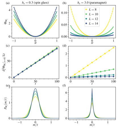
Figure 1: The dynamical potential $\Theta_{M_{z}}$ as function of $st$ for different system sizes, $L$, in the spin glass (a) and paramagnet (b) phases respectively. Note that they have opposite trends with increasing $L$ with regard to their curvature at $s=0$. The second derivative of $\Theta_{M_{z}}$ with respect to $s$ at $s=0$ as function of $t$ scaled with $L$ and $t$ suggests that $\Theta_{M_{z}}\sim s^{2}t^{2}L$ in the spin glass (c) and vanishes in the thermodynamic limit in the paramagnet (d)phase. The distribution $P_{M_{z}}(m/t)$ shows a Gaussian and exponential behaviour in the spin glass (e) and paramagnet (f) phases respectively. Other parameters are $J_{z}=0$, $J=5$, $J_{x}=0.3$, and $h=0.3$.

As mentioned in Sec. III, we can also construct the distribution $P$, moments of which yield temporal correlations of all orders. In Fig. 1(e) and (f) we show $P$ in both spin glass and paramagnetic phases using Eq. (24). They exhibit qualitatively different behaviour: while in the spin glass $P$ has a Gaussian form with standard deviation proportional to $1/\sqrt{L}$, in the paramagnetic phase the distribution has an exponential form. The origin of the Gaussian in the spin glass phase can be understood easily as the leading contribution to $\Theta_{M_{z}}$ in the thermodynamic limit is $\sim s^{2}t^{2}L$ and hence the leading contribution to $\Phi\sim m^{2}L/t^{2}$. On the other hand, in the paramagnet phase, since all derivatives of $\Theta$ with respect to $s$ at $s=0$ decrease with increasing $L$, the distribution decays exponentially away from the mean.

Note that the first derivative of $\Theta$ with respect to $s$ at $s=0$ vanishes in the both the phases, indicating that the expectation value of $M_{z}$ as a function of $t$ cannot capture the difference between the spin glass and the paramagnet phases, thus highlighting the importance of multiple-time correlations. This is also manifested in the fact that the mean of the distribution $P$ is zero in both the phases.

IV.2 Periodically driven Ising spin glass

The periodically driven cousin of the disordered Ising model (7) in the limit of $J_{x}=0$ has an exactly known phase diagram shown in Fig. 2(a) and the phases are known to be stable to the presence of interactions provided the system stays in the Floquet-many body localised phase. Since the model is driven periodically in time (with period $1$) and thus can have non-trivial temporal behaviour, we use a time-dependent $s$ of the form

$$s(t)=s\cos(\omega t),$$ (25)

and hence the potentials now have an additional parameter, namely the frequency, $\omega$, of the source field. With this form of $s(t)$, we calculate the $\Theta_{M_{z}}$ for three parameter values, corresponding to the 0-spin glass, paramagnet, and the $\pi$-spin glass, as shown by the markers in Fig. 2(a).

Since the $0$-spin glass has a phenomenology identical to the Ising spin glass discussed in Sec. IV.1, $\partial_{s}^{2}\Theta|_{s=0}\sim s^{2}n^{2}L$ ($n$ being the stroboscopic time) for $\omega\to 0$. This can be inferred from the data for $h_{x}=0.4$ from Fig. 2(b) and (c).

More interestingly, in the $\pi$-spin glass, a similar response is present for $\omega=\pi$, i.e. at half the frequency of the periodic drive and hence shows a time crystalline response (Fig. 2(b) and (e)). The response at $\omega=\pi$ can be understood quite simply from Eq. (15) as the two-time correlator $\mathcal{C}_{M_{z}}(n_{1},n_{2})$has a subharmonic response in both, $n_{1}$ and $n_{2}$. However, the more remarkable aspect is that the information of the subharmonic response in the two-time correlator survives even in an infinite temperature ensemble despite the spatial order being random over space and eigenstates.

Finally, in the paramagnet phase, since there is no spatial order anyway, there is no response at any frequency as can be seen in Fig. 2(b) and (d).

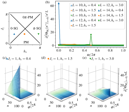
Figure 2: (a) The phase diagram of the model in Eq. (7) for $J_{x}=0$ and the markers shows the parameter values of $J_{z}$ and $h_{x}$ corresponding to which, the numerical results are shown in rest of the panels. (b) $\partial_{s}^{2}\Theta_{M_{z}}(n^{\ast})|_{s=0}/n^{\ast}L$ as function of the frequency $\omega$ at fixed time $n^{\ast}=100$ for the three different $(J_{z},h_{x})$ values marked in (a) for different $L$. The collapse of the data for different $L$ suggests that the response survives in the thermodynamic limit. (c)-(e) The behaviour of $\partial_{s}^{2}\Theta_{M_{z}}|_{s=0}/nL$ as function of $\omega$ and $n$ together shows that the integrated two-time correlator grows quadratically with time, if probed at $\omega=0$ and $\pi$ in the $0$- and $\pi$-spin glass phases respectively. Other parameters are $J=5$, $J_{x}=0.1$, $h=0.3$, and $L=14$ for (c)-(e).

V Bimodality and non-analytic potentials

In Sec. III, we saw that the probability distribution for the chosen operator (analogous to the exponential of a thermodynamic potential) is obtained from $\mathcal{Z}_{t}(s)$ of Eq. (16) (we fix $s$ to be constant for simplicity) by a Legendre transform. In a phase with a broken $\mathbb{Z}_{2}$ symmetry one might expect that the probability distribution for an appropriately chosen operator will be bimodal, analogous to a free energy landscape with a double well structure or the effective potential in a field theory Mussardo (2010). As we show later, the operator

$$G_{z}=\sum_{i\neq j}\sigma^{z}_{i}\sigma^{z}_{j},$$ (26)

is such an appropriate operator.

A practical issue is that the probability distribution obtained after a naive Legendre transform cannot be multimodal as the transform preserves convexity. In addition, we will see that the potential $\Theta$ constructed for the operator $G_{z}$ appears to be superextensive in the system size $L$. We now show that these two issues are both resolved by an appropriate splitting of $\mathcal{Z}$ inspired by the analysis of Ref. Touchette (2010) for calculating non-concave entropies in classical systems.

V.1 A toy model as a limiting case

To show how to resolve these two issues, we focus on the classical toy model defined by the limit $J_{x}=h_{\ell}=0=J_{z}$ and $J=1$ in Eq. (1) and the eigenstates of which are adiabatically connected to those in the spin-glass phase of Eq. (1) and the 0-SG phase of Sec. II. It turns out that a careful consideration of how the limits of $s\to 0$ and $L\to\infty$ (see for instance Eqs. (18) and (19)) is necessary, and the correct treatment gives a non-analytic potential and a bimodal distribution. Our analysis follows the construction of non-concave entropies in Ref. Touchette (2010).

In the infinite bond disorder limit ($J_{x}=h_{\ell}=0=J_{z}$ and $J=1$), the energy eigenstates are superpositions of pairs of product states which are $\mathbb{Z}_{2}$ flipped partners (in the $\sigma^{z}$ basis) of each other. In this limit, $G_{z}$ commutes with the Hamiltonian so that the energy eigenstates are also eigenstates of $G_{z}$. Labelling the eigenstates with $\varepsilon$ and $\pm$ analogously to Sec. II.1 and additionally by the difference between the number of up and down spins in the state, $d$, the eigenvalues of $G_{z}$ depends only upon $d$:

$$G_{z}|\varepsilon,\pm,d\rangle=\overline{G_{z}(d)}|\varepsilon,\pm,d\rangle$$ (27)

where $\overline{G_{z}(d)}=(d^{2}-L)/2$, and there are $N_{d}=\binom{L}{(L-d)/2}$ such states in the Hilbert space. The moment generating function for a finite system size $L$ is then

$$\mathcal{Z}=\frac{1}{2^{L}}\sum_{d}N_{d}e^{-st\overline{G_{z}(d)}}.$$

Calculating $\mathcal{Z}$ and $\Theta$ for a finite system reveals a problem: one can show that in this infinite bond disorder limit,

$$\partial_{s}\Theta_{G_{z}}|_{s=0} = 0,$$ (28)

$$\partial^{2}_{s}\Theta_{G_{z}}|_{s=0} = t^{2}(L^{2}-L)/2\approx t^{2}L^{2}/2$$ (29)

and hence the leading order, in $s$, term in $\Theta_{G_{z}}\approx s^{2}t^{2}L^{2}/2$ is superextensive. This is unphysical as $\Theta$ is purportedly analogous to a thermodynamic potential for the our-of-equilibrium system and hence should be extensive. The issue is resolved by the same procedure that allows for the $\phi$ (see Eq. (24)) to be non-convex. We now outline this procedure.

In our calculation the thermodynamic limit $L\rightarrow\infty$ must be taken. Since $\overline{G_{z}(d)}$ may take both positive and negative values, $-L/2\leq\overline{G_{z}(d)}\leq L(L-1)/2$, we split up $\mathcal{Z}$

$$\mathcal{Z} =\mathcal{Z}^{+}+\mathcal{Z}^{-}$$

$$=\frac{1}{2^{L}}\left[\sum_{|d|\leq\lfloor\sqrt{L}\rfloor}N_{d}e^{-st\overline{G_{z}(d)}}+\sum_{\lfloor\sqrt{L}\rfloor<|d|<L}N_{d}e^{-st\overline{G_{z}(d)}}\right],$$ (30)

where the first term consists of the eigenstates for which $\overline{G_{z}(d)}>0$ while the second $\overline{G_{z}(d)}<0$. The limit $L\rightarrow\infty$ now picks out one of the two terms depending on the sign of $s$, with $\mathrm{sgn}(s)=\pm 1$ picking out $\mathcal{Z}^{\pm}$, respectively. That is, the generating function $\mathcal{Z}$ is non-analytic in the thermodynamic limit, with

$$\Theta_{G_{z}}(s,t)\sim\begin{cases}\Theta_{G_{z}}^{+}(s,t)=\log\mathcal{Z}^{+},&s>0\\ \Theta_{G_{z}}^{-}(s,t)=\log\mathcal{Z}^{-},&s<0.\end{cases}$$ (31)

The potential is to be Legendre transformed as described in Ref. Touchette (2010): If $\Phi^{\pm}(m)$ is the Legendre transform of $\Theta^{\pm}(s)$ (as in Eq. (24)) then the correct $\Phi(m)=\max\left(\Phi^{+}(m),\Phi^{-}(m)\right)$ might be non-concave, as is the case for a bimodal probability distribution. It is also easy to show that $\Theta^{\pm}\sim\pm|s|tL$ and hence the potential is extensive.

Thus, in practice, splitting the $\mathcal{Z}$ as in Eq. (32) and taking the thermodynamic limit

• leads to a non-analytic $\Theta$ which in turns leads to a bimodal probability distribution,

• leads to extensive potentials,

and hence resolves the two issues raised at the beginning of this section. We now apply this to our quantum model.

V.2 Numerical results for the Ising spin glass

We numerically compute the potentials with the operator (26) for the Ising spin glass and show that the physics discussed in the previous subsection holds away from the toy limit of infinite bond disorder as well.

The results for the potential $\Theta_{G_{z}}$ in the spin glass and paramagnet phases are shown in Fig. 3 (a) and (b) respectively. While the curvature of $\Theta_{G_{z}}$ at $s=0$ seems to grow with increasing $L$ in the spin glass, it does not seem to depend on the system size in the paramagnet phase. To clarify this, we explicitly look at the behaviour of $\partial_{s}^{2}\Theta_{G_{z}}|_{s=0}$ in Fig. 3 (c) and (d).

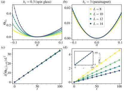
Figure 3: The potentials $\Theta_{G_{z}}$ as a function of $st$ in the spin glass (a) and the paramagnet (b) phases respectively for various $L$. The behaviour of the corresponding $\partial_{s}^{2}\Theta_{G_{z}}|_{s=0}^{/}tL^{2}$ suggests a form $\Theta_{G_{z}}\sim s^{2}t^{2}L^{2}$ in the spin glass (c) and $\sim s^{2}t^{2}L^{0}$ in the paramagnet phase (d) (see inset for collapse). Other parameters are $J_{z}=0$, $J=5$, $J_{x}=0.3$, and $h=0.3$.

Remarkably, in the spin glass the collapse of $\partial_{s}^{2}\Theta_{G_{z}}|_{s=0}/L^{2}$ for various system sizes suggests that the leading contribution to $\Theta_{G_{z}}$ is of the form $\sim s^{2}t^{2}L^{2}$. As discussed in Sec. V.1, this might seem alarming as $\mathcal{Z}$ plays the role analogous the partition function and $\Theta$, the total free energy, which in this case seems to be superextensive in $L$.

The way to resolve apparently nonphysical result that $\Theta_{G_{z}}\sim s^{2}t^{2}L^{2}$ for the full spin glass problem is then that, as discussed in Sec. V.1, the limit of $L\to\infty$ should precede $s\to 0$, as is common in the treatment of problems with spontaneously broken symmetry. As it is impossible to take the limits in that order in the numerical treatment of a finite system, we separate the sum defining $\mathcal{Z}$ into branches by analogy to the example in Sec. V.1, as follows.

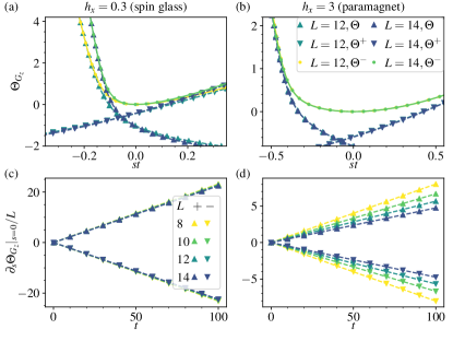
Figure 4: The branches $\Theta_{G_{z}}^{\pm}$ for the spin glass and paramagnet phases are superposed on $\Theta$ for two different system sizes for the spin glass (a) and the paramagnet (b) phases respectively. The first derivative of the branches with respect to $s$ at $s=0$ as function of $t$ and various system sizes suggests that their leading behaviour is of the form $\Theta_{G_{z}}^{\pm}\sim\pm stL$ in the spin glass (c) and $\sim stL^{-1}$ in the paramagnet (d) phase.

Consider $\{|\alpha\rangle\}$ to be complete set of basis states such that $\mathcal{Z}$ can be expressed as

$$\mathcal{Z}=\sum_{\alpha,\beta,\gamma}\langle\alpha|e^{-i\mathcal{H}^{(s)}t}|\beta\rangle\langle\beta|\rho|\gamma\rangle\langle\gamma|e^{i\mathcal{H}^{(s)\dagger}t}|\alpha\rangle.$$ (32)

The branches are then defined by restricting the summation in Eq. (32) such that $\langle\alpha|G_{z}|\beta\rangle-\langle\gamma|G_{z}|\alpha\rangle\gtrless 0$. The results for the branches computed numerically are shown in Fig. 4(a) and (b). The behaviour of the first derivative of $\Theta^{\pm}$ with respect to $s$ at $s=0$ in the spin glass phase shown in Fig. 4(c) suggests a leading behaviour of the form $\Theta_{G_{z}}^{\pm}\sim\pm stL$ which is now perfectly consistent with the effective free energy being extensive in $L$.

Thus the correct form of the potential $\Theta_{G_{z}}$ as the thermodynamic limit is approached is non-analytic in the vicinity of $s=0$, yet analytic branches can be constructed each of which is extensive in $L$. In the paramagnet phase, since the expectation of $G_{z}$ vanishes in the thermodynamic limit, the derivatives of the potential with respect to $s$ decay with increasing system size and hence the construction of branches is not necessary.

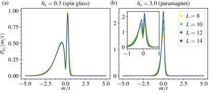
Figure 5: The distribution $P_{G_{z}}$ showing a bimodal nature in the spin glass phase (a) which seems persistent with increasing $L$ and a unimodal distribution in the paramagnet phase (b). The inset shows that if the branch construction is nevertheless used in the paramagnetic phase, one again obtains a bimodal distribution but crucial the bimodality systematically goes away with increasing $L$ eventually converging to the unimodal distribution in the thermodynamic limit.

Analogous to the construction of non-concave entropies Touchette (2010), a non-analytic $\Theta$ would suggest the presence of a non-concave and hence multimodal distribution $P$. The probability distributions are calculated from the branches individually as $P^{\pm}\sim e^{-L\phi^{\pm}}$ with $\phi^{\pm}(m,t)=-\max_{s}[sm-\theta^{\pm}(s,t)]$ and the overall probability distribution is reconstructed as $P(m,t)=max[P^{+}(m,t),P^{-}(m)]/\mathcal{N}$, where $\mathcal{N}$ is overall normalisation factor. The distributions so obtained are shown in Fig. 5. In the spin glass phase the distribution is bimodal and crucially, there is no indication of the bimodality systematically going away with increasing system size. We therefore conclude that the distribution remains bimodal in the thermodynamic limit. In the paramagnet phase, the branch construction is not used and the distribution is an unimodal one. Importantly, if one still does the branch construction in the ferromagnetic phase, a bimodal distribution is obtained for a finite system but crucially the bimodality systematically goes away with increasing $L$ (see inset of Fig. 5(b)). This establishes that in the thermodynamic limit, the true distribution is unimodal.

In conclusion, dynamical potentials for appropriate operators containing information about their temporal correlations show qualitatively different behaviours in systems with and without eigenstate order to the extent that they have different modalities, even at infinite temperature.

We note in closing that the operator $G_{z}$ can also be used similarly for the $\pi$-spin glass except it would show the bimodal distribution when probed at a frequency $\omega=\pi$.

VI Conclusion

In conclusion, we have shown that appropriate spatiotemporal correlations can reflect eigenstate order and symmetry breaking at arbitrary energy densities in infinite temperature ensembles. A probe which is completely robust to initial conditions is particularly advantageous in systems open to the environment which drives the system to a mixed state involving many eigenstates, washing out eigenstate order Medvedyeva et al. (2016); Fischer et al. (2016); Levi et al. (2016); Lazarides and Moessner (2017). It could also provide a way to get around the issue of eigenstate order getting washed out due to heating in experimental quantum simulators like cold-atom or ion-trap systems.

We then generalise the framework of Ref. Roy et al. (2017) to mixed states and show that the dynamical potentials in infinite temperature ensembles show qualitatively different behaviour in different eigenstate phases. In fact, for appropriate observables, they can also show a bimodal nature in one phase and unimodal in another.

The numerical treatment presented here is restricted to finite system sizes thus preventing us from exploring the critical points with enough accuracy. The next step in this direction is developing approximate analytical techniques, allowing access to eigenstate criticality. A natural path towards this could be recasting the moment generating functional so as to be put on the Keldysh contour. Another direction is extending this approach to open systems, in which the time evolution of interest is itself non-unitary.