Critical properties of the antiferromagnetic Ising model on rewired square lattices

Abstract

The effect of randomness on critical behavior is a crucial subject in condensed matter physics due to the the presence of impurity in any real material. We presently probe the critical behaviour of the antiferromagnetic (AF) Ising model on rewired square lattices with random connectivity. An extra link is randomly added to each site of the square lattice to connect the site to one of its next-nearest neighbours, thus having different number of connections (links). Average number of links (ANOL) $\kappa$ is fractional, varied from 2 to 3, where $\kappa=2$ associated with the native square lattice. The rewired lattices possess abundance of triangular units in which spins are frustrated due to AF interaction. The system is studied by using Monte Carlo method with Replica Exchange algorithm. Some physical quantities of interests were calculated, such as the specific heat, the staggered magnetization and the spin glass order parameter (Edward-Anderson parameter). We investigate the role played by the randomness in affecting the existing phase transition and its interplay with frustration to possibly bring any spin glass (SG) properties. We observed the low temperature magnetic ordered phase (Néel phase) preserved up to certain value of $\kappa$ and no indication of SG phase for any value of $\kappa$.

1 Introduction

The cooperative phenomena are ubiquitous in nature, driven by the presence of coupling interaction between each individual constituent of materials [1, 2]. This is exemplified by the spontaneous magnetization by which certain magnetic material is entering a ferromagnetic phase below its transition temperature $T_{c}$ (Curie temperature) and able to attract the nearby metals surrounding it. The high temperature disordered phase and the cooperative ordered phase at low temperature are separated by $T_{c}$. A phase transition is essentially rendered by the competition between the external fields, such as temperature, which tend to destroy the order and the coupling interaction which tends to create order.

Based on the nature of free energy function, a phase transition is grouped into the first and the second order phase transition[3]. The transition is called as first order if the first order derivative of the free energy of the system is discontinuous. If the derivative is continuous, the transition is second order, also called continuous phase transition, at which no latent heat involved in the course of transition and no co-existing phases[2, 4]. A firm example of these is the phase transition experienced by PVT systems above the critical point[5]. The phenomena nearby critical point are known as critical phenomena, and affected by limited number of controlling variables such as the type of coupling interaction, symmetry of the microscopic constituents (e.g., spins) and spatial dimensionality. Critical phenomena are characterized by a set of critical exponents which are in general universal, where different systems may be grouped in the same universality class, i.e., having similar value of exponents.

The type of phase transitions and universality classes are subject to the controlling variables and affected by the presence of randomness. The presence of randomness is a crucial aspect in the study of phase transition; and has long been intensively investigated. A randomness can be realized in a variety of forms such as defect (site vacancies) and diluted bonds. The effect of bond dilution for system undergoing Kosterlitz-Thouless (KT) transition has been investigated and found that the KT phase preserved so long as the bonds of the lattice are percolated[6]. According to Harris criterion[7], randomness is relevant (able to change the type or destroy the order or alter the universality classes) for the pure system experiencing second order phase transition with specific heat exponent $\alpha>0$, and irrelevant for $\alpha<0$; otherwise it is marginal.

In this study we investigated the role played by the connectivity randomness in affecting critical properties of the Ising model on rewired square lattice with AF couplings. The pure system of this model is well known to experience second order phase transition with $\alpha>0$[8]. The crucial point is that the AF couplings bring geometrical frustration due to the presence of diagonal neighbours randomly added to the square lattice. A spin is frustrated if it can not find a unique orientation in interacting with its neighbors to stay in a minimum energy state[9]. There will be an interplay between randomness and the geometrical frustration, which may affect the existing low temperature ordered phase (the Néel phase) and could possibly lead to SG ordering[10]. In fact, various spin models on rewired lattices with AF interaction have been probed in connection to SG problem[11, 12, 13]. Previously it was found that no finite temperature Ising SG phase observed on rewired square lattice for $\kappa=3$[14]. The study did not pay attention to the role played by the randomness in affecting the existing order phase. To systematically study this topic, here we consider fractional values of $\kappa$, ranging from 2 to 3. We probed the existing second order phase transition and the Néel phase at low temperature due to the presence of randomness and frustration. In particular we searched for the disappearance of AF orderings due to the increasing value of $\kappa$.

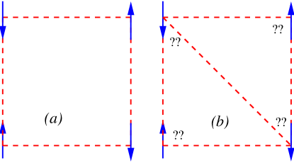
Figure 1: (a) Unfrustrated spins and (b) geometrical frustrated spins on rewired plaquettee. The AF couplings are represented by the dashed lines.

The subsequent parts of the paper is organized as follows: Section II explained the model and method. Results and discussion are presented in Section III. Section IV is devoted to the summary and concluding remarks.

2 Model and Simulation

The model is written in the following Hamiltonian

$$H=-\sum_{\langle ij\rangle}J_{ij}s_{i}s_{j}$$ (1)

where $J_{ij}$ is the coupling interaction between the Ising spin $s$ occupying respectively the site $i$-th and $j$-th of the lattice. As we probed a purely AF system, $J_{ij}=J<0$. The summation is carried out over all pairs of spins directly connecting. For regular lattices such as the square and the cubic lattice, all spins possess similar number of neighbours, associated with a fixed coordination number. Currently, we consider rewired square lattices with fractional connectivity, i.e., the average number of links (ANOL), $\kappa$, varies from 2 to 3. A rewired lattice is considered as a quasi-regular structure as the translational symmetry partially preserved. Unlike a random structure or a scale free network[15], where the notion of spatial dimension is obscure, for a quasi-regular lattice dimensionality remains. Our procedure of constructing the lattice is by randomly connecting each site to one of the diagonal neighbors of the site. There are 4 native nearest neighbors of the original square lattice; after being rewired, where one link is randomly added to each site, we obtain a lattice with fractional ANOL. Each individual site may have in minimum of 4 and maximum of 7 neighbors.

The randomly rewired lattices with AF couplings inherits the main ingredients of SG system and is considered as a new type of SG model, called non-canonical SG [11, 13, 16, 17]. It is distinguished from the canonical model as the type of randomness and frustration are not due to the presence of both FM and AF couplings. In a canonical model, both FM and AF coupling exist, while for non-canonical model only AF couplings exist, symbolically indicated by the dashed lines in Figure 1. The larger the value of $\kappa$ the larger the number of triangular units. As shown in Fig. 1, spins in AF triangular unit are frustrated. If we further add some extra links the degree of frustration of the system increases. The number of triangular units determines the degree of frustration. This is analogous to the canonical SG system with various distribution FM and AF couplings, resulting SG phase diagram with Nishimori line[18].

As a standard method in statistical mechanics, we used Monte Carlo (MC) simulation to compute the physical quantities. Due to the complexity of the energy landscape, which may be difficult to tackle using the the conventional Metropolis algorithm, here we used the Replica Exchange (RE) algorithm[19]. It is a powerful MC algorithm introduced for studying complex problems such as randomly frustrated system, in particular to overcome the problem of slow dynamics. This problem is commonly found in complex system because of the presence of local minima in the energy landscape, where a random walker can easily get trapped at certain local minimum. The basic idea of this algorithm is to extend the conventional Metropolis algorithm by duplicating the original systems into several replicas. Each replica is then independently simulated using a standard Metropolis algorithm. As each replica belongs to a heat bath with certain temperature, then the whole result of the simulation is obtained by combining each individual result. During the computation, two replicas associated with to neighboring temperatures are exchanged. This is the essential trick for the RE algorithm, by which a random walker is able to escape from any local minimum.

If we begin the simulation with a number $K$ of replicas; where every replica is in equilibrium with a heat bath of a corresponding temperature $T=1/\beta$, then the probability distribution of observing the whole system in a state $\{X\}=\{X_{1},X_{2},\dots,X_{M}\}$ is given by,

$$P(\{X,\beta\})=\prod_{m=1}^{M}\tilde{P}(X_{m},\beta_{m}),$$ (2)

with

$$\tilde{P}(X_{m},\beta_{m})=Z(\beta_{m})^{-1}\exp(-\beta_{m}H(X_{m})),$$ (3)

Here, the partition function of the m-$th$ replica is represented by $Z(\beta_{m})$. Next, we can define an exchange matrix between two replicas, $W(X_{m},\beta_{m}|X_{n},\beta_{n})$. This matrix is the probability to swap the configuration $X_{m}$ of $\beta_{m}$ with the configuration $X_{n}$ of $\beta_{n}$. In order to maintain the entire system at equilibrium, the detailed balance condition is imposed on the transition matrix

$$P(\{X_{m},\beta_{m}\},\ldots,\{X_{n},\beta_{n}\},\ldots)\cdot W(X_{m},\beta_{m}|X_{n},\beta_{n})$$

$$=P(\{X_{n},\beta_{m}\},\ldots,\{X_{m},\beta_{n}\},\ldots)\cdot W(X_{n},\beta_{m}|X_{m},\beta_{n}),$$ (4)

along with Eq. (3), so that we obtain

$$\frac{W(X_{m},\beta_{m}|X_{n},\beta_{n})}{W(X_{n},\beta_{m}|X_{m},\beta_{n})}=\exp(-\Delta),$$ (5)

where $\Delta=(\beta_{n}-\beta_{m})(H(X_{m})-H(X_{n}))$. Based on this constraint, we can choose the coefficient of matrix according to the standard Metropolis algorithm which gives the following

$$W(X_{m},\beta_{m}|X_{n},\beta_{n})=\left\{\begin{array}[]{ccc}1&{\rm if}&\Delta<0,\\ \exp(-\Delta)&{\rm if}&\Delta>0.\end{array}\right.$$ (6)

Since the ratio of acceptance ratio exponentially decays with $(\beta_{n}-\beta_{m})$, the swap is carried out only between teo adjacent temperatures, i.e., the terms $W(X_{m},\beta_{m}|X_{m+1},\beta_{m+1})$.

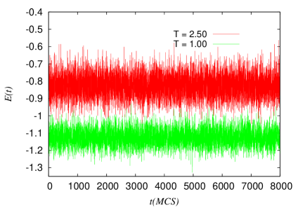
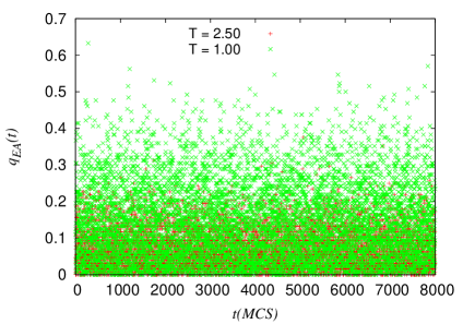
Figure 2: (Color online) Time series of enegy (left); and Edward-Anderson order parameter (right) at $T=2.50$ and $1.00$ for system size $L=16$ with $\kappa$=3.0.

In carrying out the simulation, we define a step of MC (MCS) as updating each spin once for each replica, either randomly or consecutively. After enough MCSs, we swapped each pairs of configurations belonging to neighboring temperatures according to the probability according to Eq. 6. For example, we swap replicas $X_{1}$ and and $X_{2}$, based on the probability defined Eq. 6. Then, two consecutive swaps are assigned as even and odd and. For the even swap, we exchange the pairs of replicas $X_{2}$ and $X_{3}$; $X_{4}$ and $X_{5}$; $\cdots$; $X_{M-1}$ and $X_{M}$; while for an odd one we exchange $X_{1}$ and $X_{2};\cdots X_{M-1}$ and $X_{M-3}$.

For a certain realization of connectivity, we started from a random spin configuration. Then, we equilibrated the system with $10^{4}$ MCSs before doing calculation with total of $5\times 10^{4}$ samples for each temperature. This data make up time series of corresponding physical quantities, from which we extract the thermal averages. Several additional MCSs between two samples were taken in order to avoid high time-correlation. We simulated the system with reasonable number of temperatures, so that covering the high and low temperatures. The temperature dependence of a corresponding physical quantities, apart from being averaged over samples, it is also averaged over many lattice connectivities for each system size. This is a standard procedure in MC simulation in dealing with random systems. In the next section, we present and discuss our results.

3 Results and Discussion

3.1 Time series of energy and specific heat

We have studied AF Ising model on rewired square lattices with various values of $\kappa$. Several linear sizes, $L=16,24,32$ and $48$, were simulated, with $N=L^{2}$ is the total number of sites (spins). Since the periodic boundary condition is imposed, each site of the native square lattice has the same number of nearest neighbors. For each system size we took many realizations of connectivities, then average the results over the number of realizations. Each realization corresponds to a particular connectivity distribution which is randomly generated. As a random system, results of a particular realization tend to be different from that of the other. Therefore, for a reliable result (better statistics), we took reasonable number of realizations. In previous studies on various randomly frustrated systems[16, 11, 12, 13], 1000 realizations were taken, here we took 500 realizations.

In MC simulation, time corresponds to a series of MCSs. We perform $M$ MCSs for each temperature and take a number ($N_{s}$) samples out of $M_{s}$. To check whether the system is well equilibrated, we evaluated the energy time series of the system, from which the average energy and specific heat can be extracted. The presence of any existing phase transition could be signified in the temperature dependence of specific heat. To make sure the system is well equilibrated we perform enough initial MCSs, in the order of 10⁴ MCSs, before doing measurement.

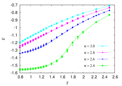
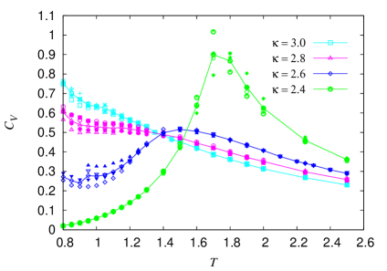
Figure 3: Temperature dependence of energy (left) and specific heat (right) of lattices with different values of $\kappa$. As shown, for $\kappa=2.4$, the specific heat is diverging, signifying a presence of second order phase transition.

The energy time series (ETS) of two different temperatures were taken, i.e., T = 2.50 and T = 1.00, for linear size $L=16$ of rewired square lattice with $\kappa=3.0$. As shown in Fig. 2, both plots indicate that system has achieved equilibrium state after a number of preliminary MCSs. Fluctuation at smaller system is more pronounced compared to larger system size. We extracted two quantities from ETS, namely the ensemble average of energy, $\langle E\rangle=\frac{1}{N}\sum_{N}E_{i}$, and the specific heat defined as follows

$$C_{v}=\frac{N}{kT^{2}}\left(\langle E^{2}\rangle-\langle E\rangle^{2}\right)$$ (7)

where $N$ and $k$ are respectively the number of spins and Boltzmann constant. These quantities are shown in Fig. 3(a) and Fig. 3(b). Each curve in the plot of average energy $\langle E\rangle$ corresponds to a system with certain $\kappa$.

The specific heat plot shown in Fig. 3 possesses a clear diverging peak for lattice with $\kappa$=2.4. This is a strong indication of the existence of phase transition. Whether this transition is related to SG phase or not can be resolved from the data of order parameter, the EA parameter and the staggered magnetization $M_{s}$ which is presented in the next sub-section. The reason of calculating $M_{s}$ is due to the fact that that the original square lattice with AF coupling, before being rewired, does experience conventional magnetic phase transition with characterized by the finite value of staggered magnetization at low temperature.

3.2 Order Parameters

To probe the interplay between randomness and geometrical frustration in affecting the existing AF magnetic order phase, we calculated two corresponding order parameters, the staggered magnetization and the overlapping parameter, also known as Edward-Anderson (EA) order parameter[21]. The former is the quantity to characterize the low temperature AF order phase, known as Néel phase; while the latter is to search for the existence SG phase. At very low temperature, the AF system on pure square lattice will have perfect Néel phase which is characterized as follows

$$M_{s}=\sum_{i}(-1)^{i}M_{i};~{}~{}~{}~{}M_{i}=\sum_{j\epsilon\{i\}}s_{j}$$ (8)

where $M_{i}$ is the magnetization of the sub-lattice$i$-th, $j$ is the spin index, depending on the sub-lattice. As here are two sub-lattices; $j$ is running from 1 to N/2; where N is the number of sites.

The EA parameter is defined as the following

$$q=q_{EA}\equiv\left[\langle|\frac{1}{N}\sum_{i}s_{i}^{(\alpha)}s_{i}^{(\beta)}|\rangle\right]_{\rm av},$$ (9)

where $s_{i}^{\alpha}$ and $s_{i}^{\beta}$ are two spin configurations with similar connectivity structure. This parameter is more like a trick in order to capture the condition of frozen configuration. Certainly, it is only relevant for numerical simulation and not relevant for experiment. It is not found in real material as almost impossible to obtain two duplicated systems with exactly the same realization of randomness. In experiment, the frozen state is measured directly by observing how the configuration change with time, in other words, one measures the time correlation of the spin configuration. The EA parameter for the Ising case is much simpler compared to the Heisenberg model which involves tensor product [11, 12]. This parameter is finite if the system is in the phase of frozen random spin configuration and vanishes otherwise.

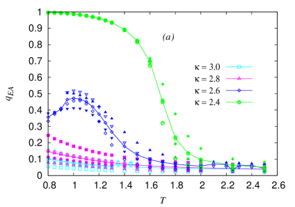
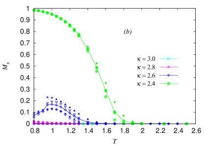
Figure 4: (a) Temperature dependence of Edward-Anderson parameter $q_{EA}$ and (b) Staggered magnetization $M_{s}$ of lattices with different values of $\kappa$. As shown, for $\kappa=2.4$, both quantities significantly increasing as temperature decreasing. The finite value of $M_{s}$ indicates a spatially ordered phase, signifies the absence of SG phase (frozen random orientation).

The temperature dependence of $q_{EA}$ for various system sizes, $L=16,24,32$ and $48$ is shown in Fig. 4(a). This parameter is to search for the existence of SG phase transition in randomly frustrated system.. We also calculated and the order parameter for AF system, the staggered magnetization $M_{s}$, shown in Fig. 4(b). The characteristics of the order parameter which increases with the decrease in temperature is the indication of phase transition. This trend is indicated by Fig. 4, where for lattice with $\kappa=2.40$, both parameters, $q_{EA}$ and $M_{s}$ are increasing. However, it is to be noticed that the increasing $q_{EA}$ can not be considered as an indication of presence of SG phase in the case $M_{s}$ also increases. SG phase which is frozen random spin orientation can not co-exist with Néel phase. Therefore, the incerasing values of both parameters indicates the existence of the same ordered phase, namely the Néel phase. The plot of $q_{EA}$ for larger value of $\kappa$, i.e, $\kappa>2.40$, indicates that this parameter increases with the decrease in temperature. However, it tends to decrease as system sizes increase. This exhibits that there is no SG phase at thermodynamic limit. The role played by the randomness, induced by random connectivity, although results in frustrated state, it fail to bring low temperature SG phase.

The absence of SG phase and the presence of AF phase at low temperature can be explained from the perspective of Harris criterion[7], which describes the role played by randomness on second order phase transition. This is exactly what observed here. The pure AF Ising model on square lattice does experience second order phase transition, with diverging specific heat. As the number of links increase, more precisely, the degree of randomness, the existing phase transition disappear at certain value of $\kappa$, i.e., around 2.7. The precise value of $\kappa$ which destroy the AF order phase at low temperature will be the subject of our next study and will be published elsewhere. With this paper, we report that non-canonical SG phase transition is not found for Ising model in the rewired square lattices with $2\leq\kappa\leq 3$.

4 Summary and Conclusion

This research studied the AF Ising model on rewired square lattices with various average number of links (ANOL), associated with coordination number for regular lattices. The lattices are obtained by randomly adding one extra link to each site of the original square lattice, lead the rewired latticess to have fractional ANOL, symbolized as $\kappa$, varied from 2 to 3. The added link is constrained to connect a site to one of its diagonal neighbors. Because of rewiring, there exist abundance of triangular units in the lattice, in which spins are frustrated due to AF couplings. Accordingly, the system under investigated is in the class of random system with geometrical frustration. We probed the role played by the randomness and frustration in affecting the existing second order phase transition of the native square lattice with AF interaction. We used Replica Exchange Monte Carlo method which is considered to be very powerful in dealing with randomly frustrated systems such as SGs. From the time series of energy, we extracted energy and calculated the specific heat. We also calculated the SG order parameter (Edward-Anderson parameter) as well as the staggered magnetization, which is the order parameter for AF ordering.

We observed a clear indication of the effect of randomness on the existing AF phase is clear and found no SG phase transition. The remnant of AF phase remains upto certain value of ANOL, i.e., $\kappa\sim 2.7$. The pure AF square lattice is associated with $\kappa=2.0$ (no extra links added) while for $\kappa=3.0$, each site has obtained one extra link. The current topic has opened another direction of research, i.e., to study the interplay between randomness rendered by rewiring procedure and the partially frustrated state. In addition, to find the lower dimension for the existence of Ising SG phase on rewired lattices is still desirable. It will be our next topic to probe, for example searching for Ising SG phase on rewired cubic lattices.

References

References

- [1] E. Ising, Z. Phys., 31, 253 (1925).
- [2] S. Sachdev, Quantum Phase Transition, 2nd. ed., Cambridge Univ. Press, (2011).
- [3] P. Ehrenfest and T. Ehrenfest, Phys. Z. 8, 311 (1907).
- [4] H. Nishimori and G. Ortiz, Elements of Phase Transition and Critical Phenomena, Oxford Univ. Press, (2011).
- [5] L. E. Reichl, A Modern Course in Statistical Physics, 2nd. John Wiley and Sons, (2009).
- [6] T. Surungan, Y. Okabe, Phys. Rev B71, 184438, (2005).
- [7] A. B. Harris, J. Phys. C 7, 1671, (1974).
- [8] C. N. Yang, Phys. Rev. 85, 808, (1952).
- [9] H. T. Diep (Ed.), Frustrated Spin Systems, 2nd. Ed., World Scientific, (2013).
- [10] V. Cannella and J. A. Mydosh, Phys. Rev. B6, 4220, (1972).
- [11] T. Surungan, F. P. Zen, and A.G. Williams, J. Phys.: Conf. Ser. 640, 012005 (2015).
- [12] T. Surungan, Bansawang BJ, D. Tahir, AIP Conf. Proc. 1719, 030006 (2016).
- [13] T. Surungan, J. Phys.: Conf. Ser. 759, 012012, (2016).
- [14] T. Surungan, J. Phys.: Conf. Ser. 988, 011001 (2018)
- [15] A.-L. Barabási and R. Albert, Science 286, 509, (1999).
- [16] M. Bartolozzi, T. Surungan, D.B. Leinweber and A.G. Williams, Phys. Rev. B73, 224419, (2006).
- [17] C. P. Herrero, Phys. Rev. E 77, 041102, (2008).
- [18] H. Nishimori, Prog. Theor. Phys. 66, 1169 (1981).
- [19] K. Hukushima and K. Nemoto, J. Phys. Soc. Japan 65, 1863, (1996).
- [20] T. Surungan, Y. Okabe, and Y. Tomita, J. Phys. A37, 4219, (2004).
- [21] S. F. Edwards and P. W. Anderson, J. Phys. F: Metal Phys. 5, 965, (1975).