Performance Analysis of Effective Methods for Solving Band Matrix SLAEs after Parabolic Nonlinear PDEs

Abstract

This paper presents an experimental performance study of implementations of three different types of algorithms for solving band matrix systems of linear algebraic equations (SLAEs) after parabolic nonlinear partial differential equations – direct, symbolic, and iterative, the former two of which were introduced in Veneva and Ayriyan (arXiv:1710.00428v2). An iterative algorithm is presented – the strongly implicit procedure (SIP), also known as the Stone method. This method uses the incomplete LU (ILU(0)) decomposition. An application of the Hotelling-Bodewig iterative algorithm is suggested as a replacement of the standard forward-backward substitutions. The upsides and the downsides of the SIP method are discussed. The complexity of all the investigated methods is presented. Performance analysis of the implementations is done using the high-performance computing (HPC) clusters “HybriLIT” and “Avitohol”. To that purpose, the experimental setup and the results from the conducted computations on the individual computer systems are presented and discussed.

1 Introduction

Systems of linear algebraic equations (SLAEs) with pentadiagonal (PD) and tridiagonal (TD) coefficient matrices arise after discretization of partial differential equations (PDEs), using finite difference methods (FDM) or finite element methods (FEM). Methods for numerical solving of SLAEs with such matrices which take into account the band structure of the matrices are needed. The methods known in the literature usually require the matrix to possess special characteristics so as the method to be stable, e.g. diagonally dominance, positive definiteness, etc. which are not always feasible.

In [1], a finite difference scheme with first-order approximation of a parabolic PDE was built that leads to a TD SLAE with a diagonally dominant coefficient matrix. The system was solved using the Thomas method (see [2]). However, a difference scheme with second-order approximation [3] leads to a matrix which does not have any of the above-mentioned special characteristics. The numerical algorithms for solving multidimensional governing equation, using FDM (e.g. alternating direction implicit (ADI) algorithms (see [4], [5])), ask for a repeated SLAE solution. This explains the importance of the existence of effective methods for the SLAE solution stage.

Two different approaches for solving SLAEs with pentadiagonal and tridiagonal coefficient matrices were explored by us in [3] – diagonal dominantization and symbolic algorithms. These approaches led to five algorithms – numerical algorithms based on LU decomposition (for PD (see [6]) and TD matrices – NPDM and NTDM), modified numerical algorithm for solving SLAEs with a PD matrix (where the sparsity of the first and the fifth diagonals was taken into account – MNPDM), and symbolic algorithms (for PD (see [6]) and TD (see [7]) matrices – SPDM and STDM). The numerical experiments with the five methods in our previous paper were conducted on a PC (OS: Fedora 25; Processor: Intel Core i7-6700 (3.40 GHz)), using compiler GCC 6.3.1 and optimization -O0. While the direct numerical methods have requirements to the coefficient matrix, the direct symbolic ones only require nonsingularity. Here, we are going to suggest an iterative numerical method which is also not restrictive on the coefficient matrix.

It is a well-known fact that solving problems of the computational linear algebra with sparse matrices is crucial for the effectiveness of most of the programs for computer modelling of processes which are described with the help of differential equations, especially when solving complex multidimensional problems. However, this is exactly how most of the computational science problems look like and hence usually they cannot be modelled on ordinary PCs for a reasonable amount of time. This enforces the usage of supercomputers and clusters for solving such big problems. For example, a numerical solving of a parabolic PDE needs to solve independently (or in parallel) $N$ SLAEs $d$ times at each time-step, where $N$ is the discretization number, i.e. the matrix dimension, and $d$ is the dimension of the PDE. Thus, it is also important to have an efficient method for serial solving of one band SLAE. Therefore, the aim and the main contribution of this paper is to investigate the performance characteristics of the considered serial methods for band SLAE being executed on modern computer clusters.

The layout of the paper is as follows: in the next section, we introduce the outline of the SIP algorithm. Afterwards, we introduce the experimental setup including the description of the computers used in our experiments and analyze the obtained results.

2 Iterative Approach

An iterative procedure for solving SLAEs with a pentadiagonal coefficient matrix is considered, namely the strongly implicit procedure (SIP) (see [8]), also known as the Stone method. It is an algorithm for solving sparse SLAEs. The method uses the incomplete LU (ILU(0)) decomposition (see [9]) which is an approximation of the exact LU decomposition in the case when a sparse matrix is considered. The idea of ILU(0) is that the zero elements of $L$ and $U$ are chosen to be on the same places as of the initial matrix $A$. In the case of a pentadiagonal coefficient matrix $A$, $LU$ is going to be also pentadiagonal, $L$ and $U$ are going to have non-zero elements only on three of their diagonals (main diagonal and two subdiagonals for $L$; main diagonal and two superdiagonals for $U$). The Stone method for solving a SLAE of the form $Ax=b$ can be seen in Algorithm 1. There, $LU$ is found using the ILU(0) algorithm suggested in [9]; $L$ and $U$ are extracted using a modification of the Doolittle method (see [4]), namely instead of referencing the matrix $A$, we reference the already found $LU$ matrix. This way the product of $L$ and $U$ is exactly $LU$.

Algorithm 1 The Stone method for solving a SLAE $Ax=b$

1:$A,b,L,U,errorMargin$

2:$k,\overrightarrow{x}^{(k)}$

3:$k=0$ $\triangleright$ number of iterations

4:$\overrightarrow{x}^{(k)}=\overrightarrow{0}$ $\triangleright$ set an initial guess vector

5:$\overrightarrow{newRHS}^{(k)}=A\,\overrightarrow{x}^{(k)}$ $\triangleright$ new right-hand side (RHS)

6:$\overrightarrow{residual}^{(k)}=\overrightarrow{b}-\overrightarrow{newRHS}^{(k)}$

7:$K=L\,U-A$

8:while $\|\overrightarrow{residual}^{(k)}\|_{\infty}\geq\textrm{errorMargin}$ do

9:     $\overrightarrow{newRHS}^{(k)}=K\,\overrightarrow{x}^{(k)}+\overrightarrow{b}$

10:     solve $L\,\overrightarrow{y}^{(k)}=\overrightarrow{newRHS}^{(k)}$

11:     solve $U\,\overrightarrow{x}^{(k+1)}=\overrightarrow{y}^{(k)}$

12:     $\overrightarrow{residual}^{(k+1)}=\overrightarrow{b}-A\,\overrightarrow{x}^{(k+1)}$

13:     $k++$

14:end while

Every iteration step of the Stone method consists of two matrix-vector multiplications with a pentadiagonal matrix, one forward and one backward substitutions with the two triangular matrices of the ILU(0), and two vector additions, i.e. the complexity of the algorithm on every iteration is $31\,N-36=O(N)$, where $N$ is the number of rows of the initial matrix.

Remark: Instead of using forward and backward substitutions on rows 10-11 of Algorithm 1, one can try to find the inverse matrices of $L$ and $U$, using a numerical procedure, e.g. the Hotelling-Bodewig iterative algorithm (see [10]). A diagonal matrix can be used as an initial guess for the inverse matrix, as it is suggested in [11]. Since a matrix implementation is going to be very demanding in regards to memory, conduction of computational experiments for a matrix with more than $7\times 10^{3}$ rows is going to be impossible. For that reason, the algorithms could be redesigned, taking into account the band structure of the data, and so an array implementation could be made. (For the Hotelling-Bodewig iterative algorithm and numerical results from that approach, see Appendix Appendix.)

3 Numerical Experiments

Computations were held on the basis of the heterogeneous computing cluster “HybriLIT” at the Laboratory of Information Technologies of the Joint Institute for Nuclear Research in town of science Dubna, Russia and on the cluster computer system “Avitohol” at the Advanced Computing and Data Centre of the Institute of Information and Communication Technologies of the Bulgarian Academy of Sciences in Sofia, Bulgaria.

3.1 Experimental Setup

The direct and iterative numerical algorithms are implemented using C++, while the symbolic algorithms are implemented using the GiNaC library (version 1.7.2) (see [12]) of C++.

The heterogeneous computing cluster “HybriLIT” consists of 13 computational nodes which include two Intel Xeon E5-2695v2 processors (12-core) or two Intel Xeon E5-2695v3 processors (14-core). For more information, visit
http://hybrilit.jinr.ru/en. It must be mentioned that for the sake of the performance analysis and the comparison between the computational times only nodes with Intel Xeon E5-2695v2 processors were used.

The supercomputer system “Avitohol” is built with HP Cluster Platform SL250S GEN8. It has two Intel 8-core Intel Xeon E5-2650 v2 8C processors each of which runs at 2.6 GHz. For more information, visit http://www.hpc.acad.bg/. “Avitohol” has been part of the TOP500 list (https://www.top500.org) twice – ranking 332nd in June 2015 and 388th in November 2015.

Tables 1 and 2 summarize the basic information about hardware, compilers and libraries used on the two computer systems. The reason why different compilers were used for the numerical and the symbolic methods, respectively, is that the GiNaC library does not maintain work with the Intel compilers. However, for the numerical methods the Intel compilers gave us better results than the GCC ones.

Computer system	Processor	Number of processors per node
“HybriLIT”	Intel Xeon E5-2695v2	2
	Intel Xeon E5-2695v3	2
“Avitohol”	Intel Xeon E5-2650v2	2

Table 1: Information about the available hardware on the two computer systems

Computer	“HybriLIT”	“Avitohol”
system
Compiler for the direct	Intel 2017.2.050 ICPC	Intel 2016.2.181 ICPC
and iterative procedures
Compiler for the	GCC 4.9.3	GCC 6.2.0
symbolic procedures
Needed libraries for the	GiNaC (1.7.2)	GiNaC (1.7.2)
symbolic procedures	CLN (1.3.4)	CLN (1.3.4)
Optimization for the direct	-O2	-O2
and iterative procedures
Optimization for the	-O0	-O0
symbolic procedures

Table 2: Information about the used software on the two computer systems

3.2 Experimental Results

During our experiments wall-clock times were collected using the member function now() of the class std::chrono::high_resolution_clock which represents the clock with the smallest tick period provided by the implementation; it requires at least standard c++11 (needs the argument -std=c++11 when compiling). We report the average time from multiple runs. Since the largest supported precision in the GiNaC library is double, during all the experiments double data type is used. The achieved accuracy during all the numerical experiments is summarized, using infinity norm. The notation is as follows: NPDM stands for numerical PD method, MNPDM – modified numerical PD method, SPDM – symbolic PD method, NTDM – numerical TD method, STDM – symbolic TD method. The error tolerance used in the iterative method is $10^{-12}$. Both the methods comprised in the iterative procedure (ILU(0) and SIP) are implemented using an array representation of the matrices instead of a matrix one.

Remark 1: So as the nonsingularity of the matrices to be checked, a fast symbolic algorithm for calculating the determinant is implemented, using the method suggested in [13]. The complexity of the algorithm is $O(N)$.

Remark 2: The number of needed operations for the Gaussian elimination used so as PD matrices to be transformed into TD ones is $18+16\,K$, where $K$ is the number of PD matrix rows with nonzero elements on their second subdiagonal and on their second superdiagonal. Usually, $K\ll N$.

The achieved computational times from solving a SLAE on “HybriLIT” are summarized in Tables 3 and 4. The number of needed iterations for the Stone method is 31.

	Wall-clock time [s]
$N$	NPDM	MNPDM	SPDM	NTDM	STDM
$10^{3}$	0.0000427	0.0000420	0.1098275	0.0000273	0.0827742
$10^{4}$	0.0004310	0.0004270	17.5189275	0.0002693	7.9570979
$10^{5}$	0.0041760	0.0040850	5991.4962896	0.0026823	2857.5483843
$10^{8}$	2.7946627	2.6662850	–	2.0525187	–
$\max\limits_{\textrm{\scriptsize{N}}}\|y-\bar{y}\|_{\infty}$	$2.22\times 10^{-16}$	$2.22\times 10^{-16}$	0	$2.22\times 10^{-16}$	0

Table 3: Results from solving a SLAE on the cluster “HybriLIT” applying direct methods.

	Wall-clock time [s]
$N$	ILU(0)	SIP
$10^{2}$	0.0004090	0.0000847
$10^{3}$	0.3493933	0.0007300
$10^{4}$	325.6368140	0.0084683
$\max\limits_{\textrm{\scriptsize{N}}}\|y-\bar{y}\|_{\infty}$	–	$1.42\times 10^{-13}$

Table 4: Results from solving a SLAE using SIP on the cluster “HybriLIT” applying an iterative method.

Tables  5 and 6 sum up the computational times from solving a SLAE on “Avitohol”. The number of needed iterations for the Stone method is 31.

	Wall-clock time [s]
$N$	NPDM	MNPDM	SPDM	NTDM	STDM
$10^{3}$	0.0000420	0.0000400	0.1089801	0.0000290	0.0518055
$10^{4}$	0.0004234	0.0004110	15.2383414	0.0002610	5.2806483
$10^{5}$	0.0040710	0.0039387	2009.6004854	0.0027417	711.9402796
$10^{8}$	2.8660797	2.7304760	–	2.1347700	–
$\max\limits_{\textrm{\scriptsize{N}}}\|y-\bar{y}\|_{\infty}$	$2.22\times 10^{-16}$	$2.22\times 10^{-16}$	0	$2.22\times 10^{-16}$	0

Table 5: Results from solving a SLAE on the supercomputer system “Avitohol” applying direct methods.

	Wall-clock time [s]
$N$	ILU(0)	SIP
$10^{2}$	0.0011817	0.0001210
$10^{3}$	0.5288667	0.0008603
$10^{4}$	516.6088950	0.0085333
$\max\limits_{\textrm{\scriptsize{N}}}\|y-\bar{y}\|_{\infty}$	–	$1.42\times 10^{-13}$

Table 6: Results from solving a SLAE using SIP on the cluster “Avitohol” applying an iterative method.

4 Discussion and Conclusions

Three different approaches for solving a SLAE are compared – direct numerical, direct symbolic, and iterative. The complexity of all the suggested numerical algorithms is $O(N)$ (see Table 7). Since it is unknown what stands behind the symbolic library, evaluating the complexity of the symbolic algorithms is a very complicated task.

Method:	NPDM	MNPDM	SPDM	NTDM	STDM	SIP
Complexity:	$19N-29$	$13N+7K-14$	–	$9N+2$	–	$31N-36$

Table 7: Complexity of the investigated methods.

Both the achieved computational times and accuracy for the NPDM and SPDM methods on both the clusters were much better than the ones outlined in [6].

All the experiments with the direct methods gave an accuracy of an order of magnitude of $10^{-16}$, while the iterative method gave an accuracy of an order of magnitude of $10^{-13}$.

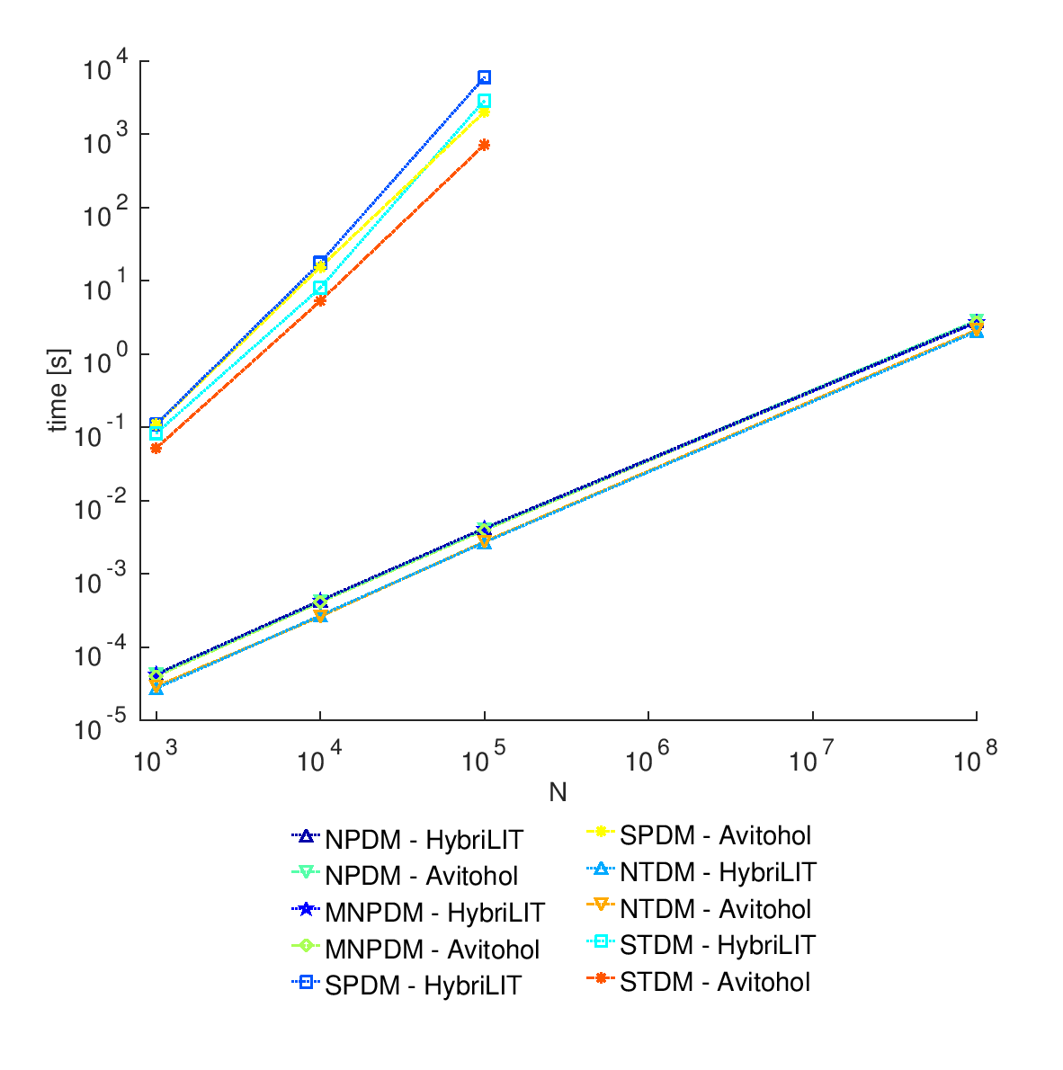
Figure 1: Execution time comparison.

Expectedly, the modified version of the numerical method for solving a SLAE with a PD matrix MNPDM gave better computational time than the general algorithm NPDM in the case of a sparse PD coefficient matrix, since the former method has a lower complexity (usually $K\ll N$, where $K$ is the number of PD matrix rows with nonzero elements on their second subdiagonal and on their second superdiagonal). The fastest numerical algorithm was found to come from the Thomas method. Finally, an iterative algorithm was built – the Stone method. For the needs of the method, additionally, ILU(0) was implemented. An upside of this iterative procedure is that it requires the initial matrix to be nonsingular only. However, this method is not suitable for matrices for which $N>1\times 10^{5}$, since the ILU(0) decomposition of a matrix is computationally demanding on time and memory. Here, likewise the symbolic algorithms, in the case of a piecewise linear parabolic partial differential equation, they do not add nonlinearity to the right-hand side of the system and hence, there is no need of iterations for the time step to be executed (see [3]). Similarly to the symbolic methods, SIP is not comparable with the numerical algorithms with respect to the required time in the case of a numerical solving of the heat equation when one needs to solve the SLAE many times. Lastly, the obtained accuracy is worse in comparison with any of the other methods. A comparison between the execution times for the direct numerical methods (see Figure 1) showed only a negligible difference between the two computer systems. However, this was not the case when it comes to the symbolic methods where “Avitohol” performed much better than “HybriLIT”. On the other hand, “HybriLIT” behaved better than “Avitohol” with respect to the ILU(0) procedure (see Figure 2). Only a minimal discrepancy in times was observed for the SIP algorithm.

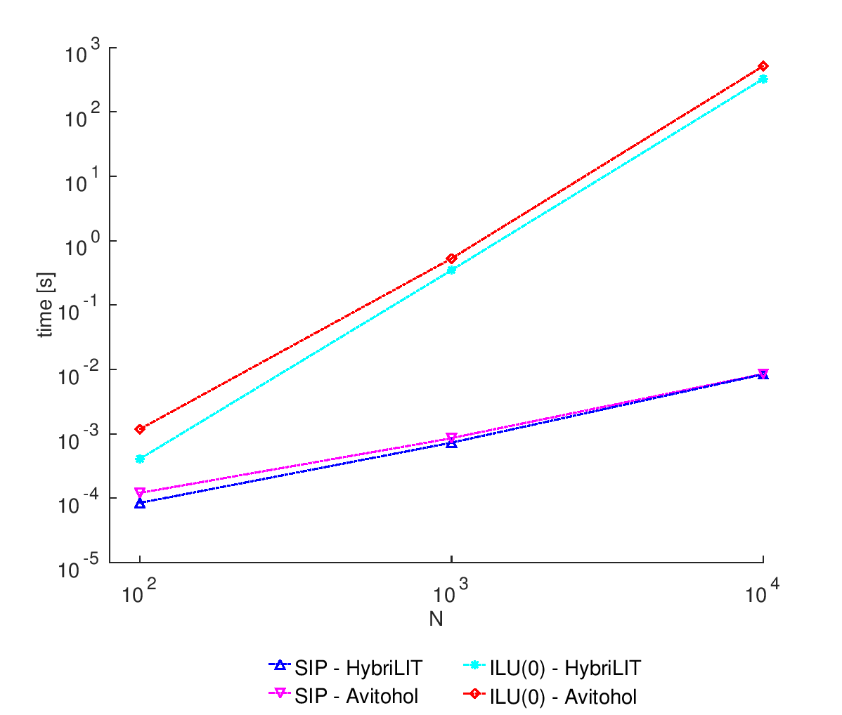
Figure 2: Execution time comparison.

Appendix

The Hotelling-Bodewig iterative algorithm has the form as follows:

$$A^{-1}_{n+1}=A^{-1}_{n}\,(2\,I-A\,A^{-1}_{n}),\quad n=0,1,\ldots,$$ (1)

where $I$ is the identity matrix, $A$ is the matrix whose inverse we are looking for. $A^{-1}_{0}$ is taken to be of a diagonal form.

The obtained computational times for the ILU(0) method, the Hotelling-Bodewig iterative algorithm and the Stone method, using the heterogeneous cluster “HybriLIT” and the supercomputer system “Avitohol”, are summarized in Tables 8, 9, and 10.

	Wall-clock time [s]
	matrix implementation			array implementation
$N$	ILU(0)	$L^{-1}$	$U^{-1}$	ILU(0)	$L^{-1}$	$U^{-1}$
$10^{2}$	0.0007027	0.0071077	0.0096933	0.0004687	0.0026583	0.0043893
$10^{3}$	1.5635590	82.9383600	49.5268260	0.3368320	3.3851580	5.3989410
$2\times 10^{3}$	21.6416160	289.3253220	300.0902740	2.5914510	27.4874390	41.7962950
$5\times 10^{3}$	547.7717120	4835.9211180	6800.0948670	39.5945850	1153.8804500	1606.9331050
$7\times 10^{3}$	1178.6338560	18966.0135900	24345.2476050	108.1988910	3395.9828320	7116.1639450
$10^{4}$	–	–	–	314.7906570	10384.6694270	14561.3854660

Table 8: Results from the ILU(0) method and the numerical method for inverting matrices, using the cluster “HybriLIT”.

	Wall-clock time [s]
	matrix implementation			array implementation
$N$	ILU(0)	$L^{-1}$	$U^{-1}$	ILU(0)	$L^{-1}$	$U^{-1}$
$10^{2}$	0.0017620	0.0089710	0.0117817	0.0013103	0.0035383	0.0060527
$10^{3}$	1.9317270	85.0694670	76.6738290	0.5320370	4.9676690	6.5183100
$2\times 10^{3}$	27.3982830	299.0649410	370.7769350	4.1901280	32.8010570	51.0338640
$5\times 10^{3}$	495.6995570	5175.7197290	6720.2701160	64.8352820	1227.5802660	1780.3281350
$7\times 10^{3}$	1144.9877790	14829.3973560	22415.4835190	177.4153890	3569.6018970	5279.6295710
$10^{4}$	–	–	–	516.4751790	10441.5862030	17833.2337200

Table 9: Results from the ILU(0) method and the numerical method for inverting matrices, using the cluster “Avitohol”.

	Wall-clock time [s]
	on “HybriLIT”		on “Avitohol”
	matrix	array	matrix	array
	implementation	implementation	implementation	implementation
$N$	SIP	SIP	SIP	SIP
$10^{2}$	0.0005637	0.0001827	0.0006510	0.0002953
$10^{3}$	0.0703420	0.0130150	0.0866850	0.0163560
$2\times 10^{3}$	0.3403310	0.0683440	0.3492530	0.0859700
$5\times 10^{3}$	2.3330770	0.5063490	3.7949870	0.5812540
$7\times 10^{3}$	8.7838330	1.1616650	6.3790020	1.2195610
$10^{4}$	–	2.0574280	–	2.9845790
$\max\limits_{\textrm{\scriptsize{N}}}\|y-\bar{y}\|_{\infty}$	$3.13\times 10^{-14}$	$3.13\times 10^{-14}$	$3.13\times 10^{-14}$	$3.13\times 10^{-14}$

Table 10: Results from solving a SLAE using SIP on the clusters “HybriLIT” and “Avitohol”.

The matrix implementations lead to 5, 7, and 34 iterations, respectively for finding $L^{-1}$ and $U^{-1}$, applying the Hotelling-Bodewig procedure, and for the Stone method while the needed iterations when the array implementations are executed are 5, 6, and 31, respectively. It is expected that inverting $L$ would require less number of iterations, since it is a unit triangular matrix. The achieved accuracy is of an order of magnitude of $10^{-13}$, having used an error tolerance $10^{-12}$. Comparing the results for the computational times, one can see that the array implementation not only decreased the time needed for the inversion of both the matrices $L$ and $U$ but also it decreases the number of iterations needed so as the matrix $U$ to be inverted. As one can see, the time required for the SIP procedure is also improved by the new implementation approach. One reason being is that the number of iterations is decreased. Overall, the array implementations decrease the computational times with one order of magnitude. Finally, this second approach requires less amount of memory (instead of keeping $N\times N$ matrix, just 5 arrays with length $N$ are stored), which allows experiments with bigger matrices to be conducted. However, this method (even in its array form) is not suitable for too large matrices (with number of rows bigger than $1\times 10^{5}$), since the evaluation of the inverse of a matrix is computationally demanding on both time and memory. A comparison between the times on the two computer systems showed that overall “HybriLIT” is a bit faster than “Avitohol”.

References

- [1] Ayriyan, A., Buša Jr., J., Donets, E. E., Grigorian, H., Pribiš, J.: Algorithm and simulation of heat conduction process for design of a thin multilayer technical device. Applied Thermal Engineering. Elsevier. 94, 151–158 (2016) doi: 10.1016/j.applthermaleng.2015.10.095
- [2] Higham, N. J.: Accuracy and Stability of Numerical Algorithms. SIAM. 2nd edn. 174–176 (2002)
- [3] Veneva, M., Ayriyan, A.: Effective Methods for Solving Band SLEs after Parabolic Nonlinear PDEs. Submitted to European Physics Journal – Web of Conferences (EPJ-WoC), arXiv: 1710.00428v2 [math.NA]
- [4] Kincaid, D. R., Cheney, E. W.: Numerical Analysis: Mathematics of Scientific Computing. American Mathematical Soc. 788 (2002)
- [5] Samarskii, A. A., Goolin, A.: Chislennye Metody. Nauka, Moscow. 45–47 (1989) (in Russian)
- [6] Askar, S. S., Karawia, A. A.: On Solving Pentadiagonal Linear Systems via Transformations. Mathematical Problems in Engineering. Hindawi Publishing Corporation. 2015, 9 (2015) doi: 10.1155/2015/232456
- [7] El-Mikkawy, M.: A Generalized Symbolic Thomas Algorithm. Applied Mathematics 3, 4, 342–345 (2012) doi: 10.4236/am.2012.34052
- [8] Stone, H. L.: Iterative Solution of Implicit Approximations of Multidimensional Partial Differential Equations. SIAM Journal of Numerical Analysis. 4, 3, 530–538 (1968) doi: 10.1137/0705044
- [9] Saad, Y.: Iterative Methods for Sparse Linear Systems. SIAM. 2nd edn. 307–310 (2003) doi: 10.1137/1.9780898718003
- [10] Schulz, G.: Iterative berechnung der reziproken matrix. Zeitschrift fur Angewandte Mathematik und Mechanik. 13 57–59 (1933) (in German)
- [11] Soleymani, F.: A Rapid Numerical Algorithm to Compute Matrix Inversion. International Journal of Mathematics and Mathematical Sciences. 2012 11 (2012) doi: 10.1155/2012/134653
- [12] Bauer, C., Frink, A., Kreckel, R.: Introduction to the GiNaC Framework for Symbolic Computation within the C++ Programming Language. J. Symbolic Computation. 33, 1–12 (2002) doi: 10.1006/jsco.2001.0494
- [13] El-Mikkawy, M.: Fast and Reliable Algorithm for Evaluating nth Order Pentadiagonal Determinants. Applied Mathematics and Computation. Elsevier. 202, 1, 210–215 (2008)