Asymptotic freedom in $\mathbbm{Z}_{2}$-Yukawa-QCD models

Abstract

$\mathbbm{Z}_{2}$-Yukawa-QCD models are a minimalistic model class with a Yukawa and a QCD-like gauge sector that exhibits a regime with asymptotic freedom in all its marginal couplings in standard perturbation theory. We discover the existence of further asymptotically free trajectories for these models by exploiting generalized boundary conditions. We construct such trajectories as quasi-fixed points for the Higgs potential within different approximation schemes. We substantiate our findings first in an effective-field-theory approach, and obtain a comprehensive picture using the functional renormalization group. We infer the existence of scaling solutions also by means of a weak-Yukawa-coupling expansion in the ultraviolet. In the same regime, we discuss the stability of the quasi-fixed point solutions for large field amplitudes. We provide further evidence for such asymptotically free theories by numerical studies using pseudo-spectral and shooting methods.

I Introduction

Gauged Yukawa models form the backbone of our description of elementary particle physics: they provide mechanisms for mass generation of gauge bosons as well as for chiral fermions via the Brout-Englert-Higgs mechanism. Many suggestions of even more fundamental theories beyond the standard model, such as grand unification, models of dark matter, supersymmetric models, etc., also involve the structures of gauged Yukawa systems. A comprehensive understanding of such systems is thus clearly indispensable.

Despite their fundamental relevance, gauged Yukawa systems can also exhibit a genuine conceptual deficiency. Many generic models develop Landau-pole singularities in their perturbative renormalization group (RG) flow towards high energies, indicating that these models may not be ultraviolet (UV) complete. If so, such models do not constitute quantum field theories which are fully consistent at any energy scale. Insisting on UV completeness by enforcing a UV cutoff to be sent to infinity typically requires to send the renormalized coupling to zero. This problem is also called triviality.

An important class of UV-complete nontrivial theories are those featuring asymptotic freedom Gross and Wilczek (1973a); Politzer (1973) which allow to send the cutoff to infinity at the expense of a vanishing bare coupling while keeping the renormalized coupling at a finite value. In fact, a conventional perturbative analysis Gross and Wilczek (1973b); Cheng et al. (1974); Gross and Wilczek (1974); Politzer (1974); Chang (1974); Chang and Perez-Mercader (1978); Fradkin and Kalashnikov (1975); Salam and Strathdee (1978); Bais and Weldon (1978); Salam and Elias (1980); Callaway (1988) is capable of revealing the existence of asymptotically free gauged Yukawa models, and allows a classification in terms of their matter content and corresponding representations. Recent studies of aspects of such models Giudice et al. (2015); Holdom et al. (2015); Hansen et al. (2017) and constructions of phenomenologically acceptable models Hetzel and Stech (2015); Pelaggi et al. (2015); Pica et al. (2016); Molgaard and Sannino (2016); Heikinheimo et al. (2017) have been performed; however, a unique route to an unequivocal model appears not obvious. Phenomenological constraints on the gauge and matter side typically require an appropriately designed scalar sector, as UV Landau poles often show up in the Higgs self-coupling.

The standard model is, in fact, not asymptotically free because of the perturbative Landau pole singularity in the U(1) gauge sector. Still, all other gauge couplings as well as the dominant top-Yukawa coupling and the Higgs self-coupling decrease towards higher energies. In fact, the value of the Higgs boson mass and the top quark mass are near-critical Buttazzo et al. (2013) in the sense that the perturbative potential approaches flatness towards the UV. Whereas a substantial amount of effort has been devoted to clarify whether the potential is exactly critical or overcritical (metastable and long-lived) in recent years Buttazzo et al. (2013); Bednyakov et al. (2015); Di Luzio et al. (2015); Andreassen et al. (2017), a conclusive answer depends on the precise value of the strong coupling and the top Yukawa coupling Alekhin et al. (2012); Bezrukov and Shaposhnikov (2015) as well as on the details of the microscopic higher-order interactions Gies et al. (2014); Branchina and Messina (2013); Hegde et al. (2014); Gies and Sondenheimer (2015); Eichhorn et al. (2015); Chu et al. (2015, 2014); Akerlund and de Forcrand (2016); Sondenheimer (2017). In summary, we interpret the present data as being compatible with the critical case of the Higgs interaction potential approaching flatness towards the UV. This viewpoint is also a common ground for the search for conformal extensions of the standard model Holthausen et al. (2013); Helmboldt et al. (2016); Ahriche et al. (2016); Shaposhnikov and Shkerin (2018).

For the present work, this viewpoint serves as a strong motivation to study asymptotically free gauged Yukawa systems. Whereas perturbation theory seems ideally suited for this, conventionally made implicit assumptions may reduce the set of asymptotically free RG trajectories visible to perturbation theory. In fact, new asymptotically free trajectories in gauged-Higgs models have been discovered with the aid of generalized boundary conditions imposed on the renormalized action Gies and Zambelli (2015, 2017). This result has also been astonishing as it was obtained in a class of models which does not exhibit asymptotic freedom in naive perturbation theory. Still, the existence of these new trajectories has been confirmed by weak-coupling approximations, effective-field-theory approaches, large-$N$ methods, as well as more comprehensively with the functional RG Gies and Zambelli (2017).

As such dramatic conclusions about the existence of new UV-complete theories requires substantiation and confirmation, the purpose of this work is to study the emergence of these new RG trajectories in a model that also exhibits asymptotic freedom already in standard perturbation theory. This allows to understand the novel features of the RG trajectories in greater detail. For this, we use the simplest gauged Yukawa system that exhibits asymptotic freedom perturbatively, it consists of a QCD-like matter sector with nonabelian SU($N_{\mathrm{c}}$) gauge symmetry Yukawa-coupled to a single real scalar field. This $\mathbbm{Z}_{2}$-Yukawa-QCD model can be viewed as a subset of the standard model Eichhorn et al. (2015); Reichert et al. (2018), with the Yukawa sector representing the Higgs boson and the top quark. In this model, the existence of asymptotically free trajectories has already been known since the seminal work of Cheng, Eichten, and Li Cheng et al. (1974) based on standard perturbation theory.

In the present work, we discover the existence of new asymptotically free trajectories in addition to the standard perturbative solution. For this, we follow the strategy of Gies and Zambelli (2015, 2017) using effective-field-theory methods and the functional RG in order to get a handle on the global properties of the Higgs potential. We generalize the approach to an inclusion of a fermionic sector and also identify a new approximation technique ($\phi^{4}$-dominance) that allows to get deeper analytical insight into the functional flow equations.

While the existence of new asymptotically free trajectories as well as some of their properties are reminiscent to the conclusions already found for the gauged-Higgs models Gies and Zambelli (2015, 2017), we also find some interesting differences. Again, the class of new solutions has free parameters, such as a field- or coupling-rescaling exponent and the location of the (rescaled) minimum of the potential during the approach to the UV. For the present $\mathbbm{Z}_{2}$-Yukawa-QCD model, we find that the exponent is more tightly constraint by the requirement of a globally stable potential. Also the rescaled potential minimum has to remain nonzero towards the UV, exemplifying the fact that the model develops a non-trivial UV structure which is not visible in the deep Euclidean region (DER). The present work thus pays special attention to the difference between working in the DER, as is often implicitly done in standard perturbation theory, and a more general analysis.

As our methods can address the global behavior of the potential, our work also adds new knowledge to the results known from standard perturbation theory: for the asymptotically free Cheng-Eichten-Li solution, we demonstrate that the potential is and remains globally stable when running the RG towards the UV; an analytic approximation of the potential can be given in terms of hypergeometric functions.

In Sec. II, we review the standard analysis of asymptotic freedom for perturbatively renormalizable $\mathbbm{Z}_{2}$-Yukawa-QCD models, for a generic number of colors and fermion flavors. We then specify our analysis to three colors and six flavors, to get closer to the standard model and only in Sec. VII, while summarizing most of our findings, we will generalize them to an arbitrary number of colors. In Sec. III, we present the functional renormalization group (FRG) approach by which we derive the RG flow equations for our model. In Sec. IV and Sec. V, we generalize the treatment of Sec. II and include perturbatively nonrenormalizable Higgs self-interactions by polynomially truncating the FRG equations, as in effective field theory (EFT) approaches, within and beyond the deep Euclidean region. In the subsequent sections we then address the task of solving the FRG equation for a generic scalar potential. In Sec. VI, we construct functional approximations of asymptotically free solutions by inspecting a regime where the scalar fluctuations are dominated by a quartic interaction. Another description is then obtained from the expansion in powers of the weak Yukawa coupling in Sec. VII. Finally in Sec. VIII, we substantiate our analytical results by using numerical tools, in particular pseudo-spectral and shooting methods. Conclusions are presented in Sec. IX.

II Asymptotic freedom within perturbative renormalizability

In the present work, we focus on a Yukawa model containing a real scalar field $\phi$ and a Dirac fermion $\psi$ which is in the fundamental representation of an $\mathrm{SU}(N_{\mathrm{c}})$ gauge group. This can be viewed as a toy model for the standard-model subsector retaining only the Higgs, the top quark, and the gluon degrees of freedom for $N_{\mathrm{c}}=3$. Its gauge-fixed classical Euclidean action reads

$$S =\int_{x}\left[\frac{1}{2}\partial_{\mu}\phi\partial^{\mu}\phi+\frac{\bar{m}}{2}\phi^{2}+\frac{\bar{\lambda}}{8}\phi^{4}+\bar{\psi}\mathrm{i}\not{D}\psi+\frac{\mathrm{i}\bar{h}}{\sqrt{2}}\phi\bar{\psi}\psi\right.$$

$$\quad\left.+\frac{1}{4}F^{i}_{\mu\nu}F^{i\mu\nu}+\frac{1}{2{\alpha}}(\partial_{\mu}A_{i}^{\mu})^{2}+\bar{\eta}^{i}\partial^{\mu}\nabla^{ij}_{\mu}\eta^{j}\right].$$ (1)

Note that this model exhibits a discrete chiral symmetry mimicking the electroweak symmetry of the standard-model Higgs sector such that a mass term for the fermion is forbidden. The top quark is coupled to the gluons through the covariant derivative $D_{\mu}=\partial_{\mu}+\mathrm{i}\bar{g}_{\mathrm{s}}A^{i}_{\mu}\tau^{i}$, with $\tau^{i}$ the generators of the $\mathrm{su}(N_{\mathrm{c}})$ Lie algebra, and to the Higgs field via the Yukawa coupling $\bar{h}$. The field strength tensor for the $\mathrm{SU}(N_{\mathrm{c}})$ gauge bosons $A^{i}_{\mu}$ is given by $F^{i}_{\mu\nu}=\partial_{\mu}A^{i}_{\nu}-\partial_{\nu}A^{i}_{\mu}-\bar{g}_{\mathrm{s}}f^{ijk}A^{j}_{\mu}A^{k}_{\nu}$ and $\nabla^{ij}_{\mu}=\delta^{ij}\partial_{\mu}+\bar{g}_{\mathrm{s}}f^{ijk}A^{k}_{\mu}$ is the covariant derivative in the adjoint representation. We adopt a Lorenz gauge with an arbitrary parameter $\alpha$ in the computation of the RG equations. We will take the Landau gauge limit ${\alpha}\to 0$ as far as the analysis of asymptotically free (AF) solutions is concerned, also because the Landau gauge is a fixed point of the RG flow of the gauge-fixing parameter Ellwanger et al. (1996); Litim and Pawlowski (1998). The gauge fixing is complemented by the use of Faddeev-Popov ghost fields $\eta^{i}$ and $\bar{\eta}^{i}$.

Let us first review the standard analysis of this model at one loop, considering only the perturbatively renormalizable couplings Cheng et al. (1974). The latter are the scalar mass $\bar{m}$, the Higgs self-interaction $\bar{\lambda}$, the Yukawa coupling $\bar{h}$ and the strong gauge coupling $\bar{g}_{\mathrm{s}}$. In particular, we address the UV behavior of this model, and look for totally AF trajectories. To this end, one focuses on the RG equations for the renormalized dimensionless couplings $g_{\mathrm{s}}$, $h$, $m$, and $\lambda$. Their definition in terms of the bare couplings and wave function renormalizations is the usual one, which we postpone to Sec. III for the moment.

As the scalar field is not charged under the gauge group, the beta function of $g_{\mathrm{s}}$ reads Gross and Wilczek (1973a)

$$\partial_{t}g_{\mathrm{s}}^{2}=\eta_{A}g_{\mathrm{s}}^{2},\quad\quad\eta_{A}=-\frac{g_{\mathrm{s}}^{2}}{8\pi^{2}}\left(\frac{11}{3}N_{\mathrm{c}}-\frac{2}{3}N_{\mathrm{f}}\right),$$ (2)

where we have allowed for in total $N_{\mathrm{f}}$ Dirac fermions in the fundamental representation. This slightly generalizes Eq. (1), where we have displayed only one Dirac field. In fact, we focus in this work on the case, where only one flavor is coupled to the scalar field via a Yukawa interaction. This is motivated by the fact that the top-Yukawa coupling plays a dominant role in the RG running of the Higgs potential and all other Yukawa couplings are negligibly small. Allowing for the presence of further Dirac fermions charged under SU($N_{\mathrm{c}}$) as in Eq. (2) does not modify the Yukawa structure. In the present section, we retain generic $N_{\mathrm{c}}$ and $N_{\mathrm{f}}$, while the following sections will specifically address $N_{\mathrm{c}}=3$ and $N_{\mathrm{f}}=6$, to mimic the standard model. In the latter case, the one-loop $\beta$ function for $g_{\mathrm{s}}$ is negative and therefore the strong coupling is AF, i.e., $g_{\mathrm{s}}^{2}\to 0$ in the UV limit.

The RG flow equation for the Yukawa coupling $h^{2}$ in this model is

$$\partial_{t}h^{2}=\frac{h^{2}}{16\pi^{2}}\left[(3+2N_{\mathrm{c}})h^{2}-6\frac{N_{\mathrm{c}}^{2}-1}{N_{\mathrm{c}}}g_{\mathrm{s}}^{2}\right].$$ (3)

The latter two equations entail that AF trajectories exist in the $(g_{\mathrm{s}}^{2},h^{2})$ plane, as it is visible in the left panel of Fig. 1, where the RG flow is represented with arrows pointing towards the UV. The dashed red line highlights a special AF trajectory, along which $h^{2}$ exhibits an asymptotic scaling proportional to $g_{\mathrm{s}}^{2}$. This behavior is best characterized in terms of the rescaled coupling

$$\hat{h}^{2}=\frac{h^{2}}{g_{\mathrm{s}}^{2}}.$$ (4)

When this ratio at some initialization scale takes the particular value

$$\hat{h}_{*}^{2}=\frac{1}{3+2N_{\mathrm{c}}}\left\{\frac{4}{3}\left(N_{\mathrm{f}}-N_{\mathrm{c}}\right)-\frac{6}{N_{\mathrm{c}}}\right\},$$ (5)

it is frozen at any RG time. Indeed the $\beta$ function of $\hat{h}^{2}$ reads

$$\partial_{t}\hat{h}^{2}=\frac{3+2N_{\mathrm{c}}}{16\pi^{2}}g_{\mathrm{s}}^{2}\hat{h}^{2}\left(\hat{h}^{2}-\hat{h}_{*}^{2}\right),$$ (6)

and it has only one nontrivial zero at $\hat{h}^{2}=\hat{h}_{*}^{2}$ for $g_{\mathrm{s}}^{2}\neq 0$. We observe that this AF trajectory exists within a finite window for $N_{\mathrm{f}}$ at fixed $N_{\mathrm{c}}$. The upper bound of the window is given by the requirement that the strong coupling constant stays AF which is essential for the considered mechanism. Beyond that upper bound, gauged-Yukawa models can still be UV complete through the mechanism of asymptotic safety, provided they feature a suitable matter content Litim and Sannino (2014); Bond and Litim (2016); Codello et al. (2016); Molgaard and Sannino (2016); Bajc and Sannino (2016). The lower bound can be obtained from Eq. (5) by demanding $\hat{h}_{*}^{2}>0$ such that $h^{2}>0$ to preserve unitarity, or reflection positivity in Euclidean signature. Thus, we obtain

$$N_{\mathrm{c}}+\frac{9}{2N_{\mathrm{c}}}<N_{\mathrm{f}}<\frac{11}{2}N_{\mathrm{c}}.$$ (7)

The standard-model case with $N_{\mathrm{c}}=3$ and $N_{\mathrm{f}}=6$ is inside this window, resulting in a fixed point at

$$\hat{h}_{*}^{2}=\frac{2}{9}.$$ (8)

A partial fixed point for a ratio of AF couplings has been called quasi-fixed point (QFP) in Ref. Gies and Zambelli (2017). It is a defining condition for AF scaling solutions and a useful tool to search for such trajectories Gross and Wilczek (1973b); Chang (1974); Callaway (1988); Giudice et al. (2015).

The fixed-point nature of Eq. (8) and its stability properties are best appreciated in the right panel of Fig. 1, where the QFP corresponds again to the dashed red trajectory.

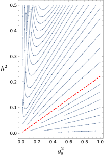
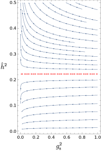
Figure 1: Left Panel: the one-loop RG flow of the perturbatively renormalizable model projected on the plane of the Yukawa coupling $h^{2}$ and the strong gauge coupling $g_{\mathrm{s}}^{2}$. The color and flavor numbers are fixed to $N_{\mathrm{c}}=3$ and $N_{\mathrm{f}}=6$. Right panel: the same flow plotted in terms of the rescaled Yukawa coupling $\hat{h}^{2}$ defined in Eq. (4). The UV repulsive QFP is highlighted by a red dashed line that corresponds to the solution of Eq. (8).

Using the flow in theory space in terms of $\hat{h}^{2}$, this trajectory classifies as UV unstable. UV-complete trajectories hence have to emanate from the QFP. In turn, these trajectories are IR attractive, hence the low-energy behavior is governed by the QFP, enhancing the predictive power of the model.

From another perspective, the AF trajectory defined by Eq. (8) can be viewed as an upper bound on the ratio of the Yukawa coupling and the gauge coupling at some initializing scale. For $\hat{h}^{2}>\hat{h}_{*}^{2}$, asymptotic freedom is lost and the Yukawa coupling hits a Landau pole at a finite RG time towards the UV. The Yukawa coupling becomes AF only for $\hat{h}^{2}\leq\hat{h}_{*}^{2}$. Throughout the main text of this work, we will concentrate on the implications of the RG flow for the particular ratio defined by this upper bound where the flow of the Yukawa coupling is locked to the running of $g_{\mathrm{s}}$. For $\hat{h}^{2}<\hat{h}_{*}^{2}$, the Yukawa coupling is driven faster than the gauge coupling towards the Gaußian fixed point for high energies. These scaling solutions are sketched in App. A.

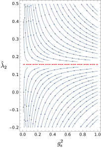
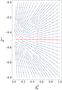
Figure 2: The one-loop RG flow of the perturbatively renormalizable model projected on the plane of the rescaled Higgs quartic coupling $\hat{\lambda}_{2}$ (for $P=1/2$ as defined in Eq. (11)) and the strong gauge coupling $g_{\mathrm{s}}^{2}$. The color and flavor numbers are fixed to $N_{\mathrm{c}}=3$ and $N_{\mathrm{f}}=6$. The UV repulsive QFP $\hat{\lambda}_{2}^{+}$ in the left panel and the UV attractive QFP $\hat{\lambda}_{2}^{-}$ in the right panel are highlighted by red dashed lines that correspond to the solutions in Eq. (16).

In order to investigate the implications for the Higgs sector, we first study the $\beta$ function for the renormalized quartic coupling at the one-loop level

$$\partial_{t}\lambda = \frac{9}{16\pi^{2}}\lambda^{2}-\frac{N_{\mathrm{c}}}{4\pi^{2}}h^{4}+2\eta_{\phi}\lambda,$$ (9)

$$\eta_{\phi} = \frac{N_{\mathrm{c}}}{8\pi^{2}}h^{2},$$ (10)

where $\eta_{\phi}$ is the anomalous dimension of the scalar field. We would like to emphasize at this point that we restrict the discussion to the deep Euclidean region (DER) here, where all the masses are negligible compared to the RG scale. This implies in particular that any threshold effect given by the mass parameter $m$ of the scalar field is neglected. In case the system is in the symmetry-broken regime, effects from a nonvanishing vacuum expectation value on the properties of the top quark are also ignored for the moment, as they would alter the beta functions for the Yukawa coupling and the gauge coupling as well.

The $\beta$ function for the quartic coupling is a parabola with two roots that are proportional to $h^{2}$. As before, we classify AF trajectories by a QFP condition for a suitable ratio

$$\hat{\lambda}_{2}=\frac{\lambda}{h^{4P}},\quad P>0,$$ (11)

where the power $P$ is determined by the requirement that $\hat{\lambda}_{2}$ achieves a finite positive value in the UV. The flow equation for this rescaled Higgs coupling then receives contributions from the $\beta$ function of $h^{2}$. As already stated, we focus on the AF trajectories with $\hat{h}^{2}=\hat{h}_{*}^{2}$. In this case it is convenient to define an anomalous dimension for the Yukawa coupling by

$$\eta_{h^{2}}\equiv\left.-\frac{\partial_{t}h^{2}}{h^{2}}\right|_{h^{2}=g_{\mathrm{s}}^{2}\hat{h}_{*}^{2}}=-\eta_{A},$$ (12)

which is related to the anomalous dimension of the gauge field as $h^{2}\sim g_{\mathrm{s}}^{2}$ for this specific trajectory. Moreover, it is useful to introduce two rescaled anomalous dimensions, by factoring out the Yukawa coupling

$$\hat{\eta}_{h^{2}} = \frac{\eta_{h^{2}}}{h^{2}}=\frac{1}{8\pi^{2}\,\hat{h}_{*}^{2}}\left(\frac{11}{3}N_{\mathrm{c}}-\frac{2}{3}N_{\mathrm{f}}\right)\,,$$ (13)

$$\hat{\eta}_{\phi} = \frac{\eta_{\phi}}{h^{2}}=\frac{N_{\mathrm{c}}}{8\pi^{2}}.$$ (14)

It turns out that the only possible QFP occurs at $P=1/2$, as suggested by the scaling of the two roots of Eq. (9). In this case the $\beta$ function of the rescaled Higgs coupling reads

$$\partial_{t}\hat{\lambda}_{2}=h^{2}\!\left(\frac{9}{16\pi^{2}}\hat{\lambda}_{2}^{2}+\left(2\hat{\eta}_{\phi}+\hat{\eta}_{h^{2}}\right)\hat{\lambda}_{2}-\frac{N_{\mathrm{c}}}{4\pi^{2}}\right).\ \$$ (15)

In fact for $P=1/2$ the QFP equation $\partial_{t}\hat{\lambda}_{2}=0$ admits two real roots, one positive and one negative. For instance, choosing $N_{\mathrm{c}}=3$ and $N_{\mathrm{f}}=6$ results in

$$\hat{\lambda}_{2}^{\pm}=\frac{1}{6}\left(-25\pm\sqrt{673}\right).$$ (16)

The $\beta$ function for $\hat{\lambda}_{2}$ is a convex parabola, therefore the positive (negative) root corresponds to a UV repulsive (attractive) QFP. The phase diagram is depicted in Fig. 2. Exactly on top of $\hat{\lambda}_{2}^{+}$ the Yukawa coupling drives the Higgs coupling to zero towards the UV. For an initial condition such that the rescaled scalar coupling is smaller than $\hat{\lambda}_{2}^{+}$, $\hat{\lambda}_{2}$ is attracted in the UV towards the negative root and the perturbative potential appears to become unstable. For an initial value bigger than $\hat{\lambda}_{2}^{+}$, the scalar coupling hits a Landau pole in the UV. Hence, the requirement of a stable and UV-complete theory enforces $\hat{\lambda}_{2}=\hat{\lambda}_{2}^{+}$. As for the Yukawa coupling, this trajectory is IR attractive, hence the low-energy behavior is governed by the QFP $\hat{\lambda}_{2}^{+}$. Thus, the theory exhibits a higher degree of predictivity.

In the remaining part of this paper, we restrict ourselves to an asymptotic UV running of the Yukawa coupling described by Eq. (4) and Eq. (5). We will refer to the AF solution described by Eq. (5) and by the positive root in Eq. (16) as the Cheng–Eichten–Li (CEL) solution, since it was first described in Ref. Cheng et al. (1974). The further AF solutions with $\hat{h}^{2}<\hat{h}_{*}^{2}$ have also already been discussed in Ref. Cheng et al. (1974) as well as in later analyses Chang (1974); Giudice et al. (2015); for completeness, we review them in App. A. For the remainder of the paper, we consider the asymptotic UV running of the Yukawa coupling of Eqs. (4) and (5), because it is most predictive: whereas classically the gauge coupling $g_{\mathrm{s}}$, the Yukawa coupling $h$ and the scalar self-interaction $\lambda$ are independent, our AF trajectory locks the running of $h$ and $\lambda$ to that of $g_{\mathrm{s}}$. Physically, this implies that the mass of the fermion (top quark) as well as that of the Higgs boson will be determined in terms of the initial conditions for the gauge sector and the scalar mass-like parameter, i.e., the Fermi scale. This maximally predictive point in theory space is also called the Pendleton-Ross point Pendleton and Ross (1981). Let us finally emphasize that we focus exclusively on the UV behavior of our model class in the present work. The low-energy behavior will be characterized by possible top-mass generation from $\mathbbm{Z}_{2}$ symmetry breaking and a QCD-like low-energy sector for the remaining fermion flavors and gauge degrees of freedom. In models with a gauged Higgs field, a distinction of Higgs- and QCD-like phases as well as details of the particle spectrum might be much more intricate Maas (2013); Maas and Mufti (2015); Maas et al. (2017); Maas (2017).

The question that is left open by the preceding standard perturbative UV analysis is as to whether the CEL solution is the only possible AF model with the same field content and symmetries of Eq. (1). More specifically, can there be more AF solutions outside the family of perturbatively renormalizable models? To address this possibility, we take inspiration from the discovery that new AF trajectories can be constructed in nonabelian Higgs models, if functional RG equations are used to explore the space of theories including also couplings with negative mass dimension Gies and Zambelli (2015, 2017). Therefore, as a first step of our investigation, we now turn to the computation of such functional RG equations for $\mathbbm{Z}_{2}$-Yukawa-QCD models.

III Functional renormalization group

Since the work of Wilson, Wegner and Houghton, it is known that in a generic field theory one can construct functional RG equations which are exact Wilson and Kogut (1974); Wegner and Houghton (1973). For many purposes, the most useful form of these equations is the one, referring to the one-particle irreducible effective action $\Gamma$, which descends from adding a regularization kernel $R_{k}$ to the quadratic part of the bare action, in order to keep track of the successive inclusion of IR modes at a scale $k$. Then the full (inverse) two-point function $\Gamma_{k}^{(2)}$ at this scale enters the one-loop computation, supplemented by the regulator $R_{k}$. Differentiating with respect to the scale $k$ leads to the Wetterich equation Wetterich (1993); Ellwanger (1994); Morris (1994a); Bonini et al. (1993)

$$\partial_{t}\Gamma_{k}[\Phi]=\frac{1}{2}\text{STr}\left\{\frac{\partial_{t}R_{k}}{\Gamma^{(2)}_{k}[\Phi]+R_{k}}\right\}\,,$$ (17)

where $t=\log(k/k_{\mathrm{ref}})$ is the RG time with $k_{\mathrm{ref}}$ some reference scale. Thanks to the derivative $\partial_{t}R_{k}$ in the numerator, all UV divergences are regulated as well. The effective average action $\Gamma_{k}$ interpolates between a microscopic theory defined at some UV scale $\Lambda$, $\Gamma_{k=\Lambda}=S_{\text{cl}}$, and the effective action $\Gamma_{k=0}=\Gamma$, where all the quantum fluctuations are integrated out, see Berges et al. (2002); Pawlowski (2007); Gies (2012); Delamotte (2012); Braun (2012) for reviews.

Equation (17) can be projected onto the RG flow of a specific coupling constant. In addition, it is also well suited to study functional parametrizations of the dynamics, such as a general scalar effective potential. These functional flow equations can then be used also outside the regime of small field amplitudes, to address problems such as the existence of a nontrivial minimum or the global stability of the theory.

As we are interested in the properties of the beta functional of the scalar potential, we use

$$\Gamma_{k} =\int_{x}\left[\frac{Z_{\phi}}{2}\partial_{\mu}\phi\partial^{\mu}\phi+U\left(\phi^{2}/2\right)+Z_{\psi}\bar{\psi}\mathrm{i}\not{D}\psi+\frac{\mathrm{i}\bar{h}}{\sqrt{2}}\phi\bar{\psi}\psi\right.$$

$$\quad\left.+\frac{Z_{A}}{4}F^{i}_{\mu\nu}F_{i}^{\mu\nu}+\frac{Z_{A}}{2{\alpha}}(\partial_{\mu}A_{i}^{\mu})^{2}+Z_{\eta}\bar{\eta}^{i}\partial_{\mu}\nabla_{ij}^{\mu}\eta^{j}\right],$$ (18)

as an approximation scheme for the effective average action. This derivative expansion has proven useful, especially in the analysis of the RG flow of the Higgs potential Gies et al. (2013, 2014); Gies and Sondenheimer (2015); Eichhorn and Scherer (2014); Eichhorn et al. (2015); Gies and Zambelli (2015); Jakovac et al. (2016a, b); Vacca and Zambelli (2015); Borchardt et al. (2016); Gies and Zambelli (2017); Jakovác et al. (2017); Gies et al. (2017); Gies and Sondenheimer (2017); Sondenheimer (2017). The effective average potential $U$ which exhibits a discrete $\mathbb{Z}_{2}$ symmetry and the wave function renormalizations $Z_{\{\phi,\psi,A,\eta\}}$ are scale dependent, as well as the Yukawa coupling $h^{2}$ and the strong coupling $g_{\mathrm{s}}$. Let us introduce a dimensionless renormalized scalar field in order to fix the usual RG invariance of field rescalings

$$2\rho=Z_{\phi}k^{2-d}\phi^{2}.$$ (19)

In a similar manner, also renormalized fields for the fermions and the gauge bosons might be introduced. The dimensionless renormalized couplings read

$$h^{2}=\frac{\bar{h}^{2}k^{d-4}}{Z_{\phi}Z_{\psi}^{2}},\quad g_{\mathrm{s}}^{2}=\frac{\bar{g}_{\mathrm{s}}^{2}k^{d-4}}{Z_{A}}.$$ (20)

By plugging the ansatz for $\Gamma_{k}$ into Eq. (17), we can extract the flow equations for the dimensionless potential

$$u(\rho)=k^{-d}U(Z_{\phi}^{-1}k^{d-2}\rho),$$ (21)

as well as the flow equation for the dimensionless renormalized Yukawa coupling, $\partial_{t}h^{2}$. Similarly, we obtain the anomalous dimensions of the fields that are defined as

$$\eta_{\phi}=-\partial_{t}\log Z_{\phi},\quad\quad\eta_{\psi}=-\partial_{t}\log Z_{\psi},$$ (22)

encoding the running of the wave function renormalizations.

The functional flow equation for the full dimensionless renormalized potential is given by

$$\partial_{t}u =-du(\rho)+(d-2+\eta_{\phi})\rho u^{\prime}(\rho)+2v_{d}\,l_{0}^{(\mathrm{B})d}(\omega,\eta_{\phi})$$

$$\quad-2v_{d}N_{\mathrm{c}}d_{\gamma}\,l_{0}^{(\mathrm{F})d}(\omega_{1},\eta_{\psi}),$$ (23)

where $v_{d}^{-1}=2^{d+1}\pi^{d/2}\Gamma(d/2)$ and $\omega$ as well as $\omega_{1}$ are defined as

$$\begin{split}\omega=u^{\prime}(\rho)+2\rho u^{\prime\prime}(\rho),\quad\omega_{1}=h^{2}\rho.\end{split}$$ (24)

Moreover, we have ignored field-independent contributions coming from a pure gluon or ghost loop which are irrelevant for the following investigations. The threshold functions $l_{0}^{(\mathrm{B})d}$ and $l_{0}^{(\mathrm{F})d}$ encode the nonuniversal regulator dependence of loop integrals and describe the decoupling of massive modes. Their general definitions as well as explicit representations for a convenient piece-wise linear regulator Litim (2000, 2001) to be used in the following, are listed, for instance, in Ref. Gies et al. (2017). Of course, it is straightforward to derive flow equations for particular scalar self-couplings up to an arbitrary order from this beta functional for the scalar potential. Additionally, it contains information beyond the RG evolution of polynomial approximations of the effective potential and keeps track of all relevant scales, the field amplitude as well as the RG scale. Thus, it allows to study global properties of the Higgs potential which we will discuss with regard to AF trajectories in the following.

The flow equation for the Yukawa coupling extracted from the Wetterich equation reads

$$\partial_{t}h^{2} =(d-4+\eta_{\phi}+2\eta_{\psi})h^{2}+4v_{d}h^{4}\,l_{11}^{(\mathrm{F}\mathrm{B})d}(\omega_{1},\omega;\eta_{\psi},\eta_{\phi})$$

$$\quad-\frac{N_{\mathrm{c}}^{2}-1}{2N_{c}}(d+{\alpha}-1)8v_{d}\,h^{2}g_{\mathrm{s}}^{2}\times$$

$$\quad\times l_{11}^{(\mathrm{F}\mathrm{B})d}(\omega_{1},0;\eta_{\psi},\eta_{A})|_{\rho=\kappa}.$$ (25)

Note, that this flow equation differs in the SSB regime from the one which was usually adopted in the literature for Yukawa models, e.g., Gies et al. (2014); Gies and Sondenheimer (2015). It has turned out that the running of $h$ extracted from a projection onto a field-dependent two-point function $\Gamma^{(2)}_{\bar{\psi}\psi}(\phi)$ shows better convergence upon the inclusion of higher-dimensional Yukawa interactions than the projection onto the three-point function $\Gamma^{(3)}_{\phi\bar{\psi}\psi}$ in case the system is in the SSB regime Pawlowski and Rennecke (2014); Gies et al. (2017). The flow equation for the Yukawa coupling extracted from $\Gamma^{(3)}_{\phi\bar{\psi}\psi}$ can be obtained from Eq. (25) by taking a derivative with respect to $\rho$ before evaluating at $\rho=\kappa$ which coincides with flow equation $\partial_{t}h^{2}$ derived in Gies et al. (2014).

Finally, the scalar and spinor anomalous dimensions read

$$\eta_{\phi} =\frac{8v_{d}\kappa}{d}\big{[}3u^{\prime\prime}(\rho)+2\kappa u^{\prime\prime\prime}(\rho)\big{]}^{2}\,m_{2}^{(B)d}(\omega,\eta_{\phi})$$

$$\quad+\frac{4v_{d}N_{\mathrm{c}}d_{\gamma}h^{2}}{d}\Big{[}m_{4}^{(F)d}(\omega_{1},\eta_{\psi})$$

$$\qquad\qquad\qquad\qquad-h^{2}\kappa\,m_{2}^{(F)d}(\omega_{1},\eta_{\psi})\Big{]}\Big{|}_{\rho=\kappa},$$ (26)

and

$$\eta_{\psi} =\frac{4v_{d}h^{2}}{d}m_{12}^{(FB)d}(\omega_{1},\omega;\eta_{\psi},\eta_{\phi})$$

$$\quad+\frac{8v_{d}}{d}\frac{N_{\mathrm{c}}^{2}-1}{2N_{\mathrm{c}}}g_{\mathrm{s}}^{2}\bigl{[}(d-{\alpha}-1)m_{12}^{(FB)d}(\omega_{1},0;\eta_{\psi},\eta_{A})$$

$$\quad-(d-1)(1-{\alpha})\tilde{m}_{11}^{(FB)d}(\omega_{1},0;\eta_{\psi},\eta_{A})\bigr{]}\big{|}_{\rho=\kappa},$$ (27)

with further threshold functions $m_{\dots}^{\dots}$ and $\tilde{m}_{\dots}^{\dots}$. Their arguments $\omega$ and $\omega_{1}$ in Eqs. (26) and (27) are evaluated at the minimum of the potential $\kappa$, which means $\kappa=0$ in the symmetric regime and $u^{\prime}(\kappa)=0$ in the SSB regime. The precise definitions for all the threshold functions can be found in Gies et al. (2017). For our quantitative analysis, we use the Landau gauge ${\alpha}\to 0$, and a piece-wise linear regulator Litim (2000, 2001) for convenience.

In principle, functional flow equations can also be obtained for the gauge sector of the model. Nevertheless as we are interested in the properties of the flow equations far above the QCD scale where $g_{\mathrm{s}}$ is small, it is legitimate to treat the running of the gauge sector in a standard way. Therefore we will use the one-loop beta function for $g_{\mathrm{s}}$ as shown in Eq. (2).

As a matter of course, the universal one-loop coefficients of the beta function for the Yukawa as well as the quartic Higgs coupling and the one-loop expressions for the anomalous dimensions can be extracted from the flow Eqs. (23)-(27). For this purpose, one has to set all the anomalous dimensions occurring in the threshold functions to zero, but keep the anomalous dimensions entering the dimensional scaling of the renormalized couplings. The latter contribute to the perturbative one-loop flow equation via one-particle reducible graphs. Furthermore, one has to take the limit toward the DER, by setting the mass parameter as well as the scalar vacuum expectation value to zero to neglect threshold effects. Then, the anomalous dimension of the scalar field reduces to Eq. (10), and we obtain

$$\eta_{\psi}=\frac{h^{2}}{32\pi^{2}}\equiv h^{2}\hat{\eta}_{\psi},$$ (28)

for the spinor anomalous dimension in the Landau gauge at one-loop order in $d=4$. The flow equation for the Yukawa model reads in this limit

$$\partial_{t}h^{2} =(\eta_{\phi}+2\eta_{\psi})h^{2}+\frac{h^{4}}{8\pi^{2}}-\frac{3}{8\pi^{2}}\frac{N_{\mathrm{c}}^{2}-1}{N_{c}}h^{2}g_{\mathrm{s}}^{2}.$$ (29)

Using the one-loop expressions for the anomalous dimensions, we obtain Eq. (3). In the rest of this paper we will drop the index $d$ from the threshold functions, as we work in $d=4$ from now on.

The freedom to choose different regularization schemes is parametrized by the threshold functions $l,m,\dots$. This includes general mass-dependent schemes as well as mass-independent schemes as a particular limiting case. Using an EFT-like analysis, we investigate in the following whether the results in the more general mass-dependent schemes are sensitive to the assumption of working in the DER as a special case. It turns out below that the restriction to the DER is severe and legitimate only for the CEL solution. A more general class of asymptotically free solutions requires to take threshold effects into account.

IV Effective field theory analysis in the deep Euclidean region

In the present section and Sec. V, we discuss a generalization of the construction outlined in Sec. II, by including perturbatively nonrenormalizable interactions. In adding higher-dimensional operators to Eq. (1), we follow the EFT paradigm, but we do so only for momentum-independent scalar self-interactions. In fact, as will be explained in the next sections, a justification of the consistency of the new AF solutions we construct requires an infinite number of higher-dimensional operators, which cannot be generally dealt with, unless further restrictions are imposed. The focus on point-like scalar self-interactions is one such additional specification, and it will be extensively discussed in the following.

Regardless of our choice to depart from a standard EFT setup, the AF solutions can be studied also within the latter. The goal of the present section and of Sec. V is precisely to explain how to reveal these solutions and to properly account for some of their properties in a parameterization where a finite number of couplings with higher dimension is included. These steps can be followed also when all interactions up to some given dimensionality are included in the effective Lagrangian. Still, the crucial ingredient in the construction is a treatment of the $\beta$ functions of these operators that slightly differs from the standard EFT one. Namely, one has to treat the scale dependence of one coupling or Wilson coefficient in the EFT expansion as free. Finally, we will show in the next sections that this additional freedom has to be present in any rigorous definition of the RG flow of the model, due to the infinite dimensionality of the theory space, and plays the role of a boundary condition in a functional representation of the quantum dynamics.

Let us start detailing the EFT-like analysis of the RG flow for the dimensionless potential. To this end, we consider a systematic polynomial expansion of $u(\rho)$ around the actual scale-dependent flowing minimum $\kappa$, which can be either at vanishing field amplitude (SYM regime) or at some nontrivial value (SSB regime). Assuming that the system is in the SSB regime, the potential is parametrized as

$$u(\rho)=\sum_{n=2}^{N_{\mathrm{p}}}\frac{\lambda_{n}}{n!}(\rho-\kappa)^{n}.$$ (30)

Generically, we expect all couplings to be generated by fluctuations, i.e., $N_{\mathrm{p}}\to\infty$, whereas truncating the sum at some finite $N_{\mathrm{p}}$ corresponds to a polynomial approximation of the potential.

As we said above, in the present section we first study the DER where all mass parameters are neglected. To implement this regime we restrict our analysis to the limit $\kappa\to 0$. This ansatz is then plugged into Eq. (23) such that, by setting the anomalous dimensions inside the threshold functions to zero, we recover the set of one-loop $\beta$ functions $\partial_{t}\lambda_{n}$ for $n=2,\dots,N_{\mathrm{p}}$ in the DER. As we are interested in constructing AF trajectories, we allow for any arbitrary scaling of the quartic coupling $\lambda_{2}$ with respect to the AF Yukawa coupling $h^{2}$, and introduce the finite ratio $\hat{\lambda}_{2}$ defined in Eq. (11) for $\lambda=\lambda_{2}$. Any QFP for $\hat{\lambda}_{2}$ at a finite nonvanishing value of $h^{2}$ has the interpretation of an AF scaling solution for $\lambda_{2}$. Similar arguments can be applied to the higher-order couplings $\lambda_{n}$, suggesting to define

$$\hat{\lambda}_{n}=\frac{\lambda_{n}}{h^{2P_{n}}},$$ (31)

with $P_{2}=2P$, cf. Eq. (11).

Concerning the scaling of the Higgs coupling, namely the power $P$ of Eq. (11), it will become clear soon that the only possibility in the DER is $P=1/2$. In fact, since $\hat{\lambda}_{3}$ and $\hat{\lambda}_{4}$ contribute to the $\beta$ function of $\hat{\lambda}_{2}$, $P$ cannot be fixed without fixing simultaneously all the other powers $P_{n}$ with $n>2$. To simplify the discussion, we already start with the ansatz $P=1/2$ and look for the corresponding values of $P_{n}$ and $\hat{\lambda}_{n}$. The flow equation for $\hat{\lambda}_{3}$ then reads

$$\partial_{t}\hat{\lambda}_{3}=-\frac{81}{16\pi^{2}}\hat{\lambda}_{2}^{3}h^{2(3-P_{3})}+\frac{9}{4\pi^{2}}h^{2(3-P_{3})}+2\hat{\lambda}_{3}+\mathcal{O}(h^{2}),$$

thus a QFP solution with finite $\hat{\lambda}_{2}$ and $\hat{\lambda}_{3}$ is possible only for $P_{3}=3$. In the same way it is possible to fix the scaling of all the higher order couplings, and to conclude that

$$P=\frac{1}{2}\quad\text{and}\quad P_{n>2}=n.$$ (32)

The truncation of the polynomial expansion in Eq. (30) up to some integer value for $N_{\mathrm{p}}$ and for $\kappa=0$, provides a system of $N_{\mathrm{p}}$ equations in $N_{\mathrm{p}}$ variables when one looks at the QFP condition. To give an example, the first four beta functions are shown here to leading order in $h^{2}$:

$$\partial_{t}\hat{\lambda}_{2} =h^{2}\left(\frac{9}{16\pi^{2}}\hat{\lambda}_{2}^{2}+\frac{75}{16\pi^{2}}\hat{\lambda}_{2}-\frac{3}{4\pi^{2}}\right)+\mathcal{O}(h^{4})$$

$$\partial_{t}\hat{\lambda}_{3} =2\hat{\lambda}_{3}-\frac{81}{16\pi^{2}}\hat{\lambda}_{2}^{3}+\frac{9}{4\pi^{2}}+\mathcal{O}(h^{2})$$

$$\partial_{t}\hat{\lambda}_{4} =4\hat{\lambda}_{4}+\frac{243}{4\pi^{2}}\hat{\lambda}_{2}^{4}-\frac{9}{\pi^{2}}+\mathcal{O}(h^{2})$$

$$\partial_{t}\hat{\lambda}_{5} =6\hat{\lambda}_{5}-\frac{3645}{4\pi^{2}}\hat{\lambda}_{2}^{5}+\frac{45}{\pi^{2}}+\mathcal{O}(h^{2}).$$ (33)

By neglecting the subleading contributions, we have that the QFP solution for the scalar quartic coupling is $\hat{\lambda}_{2}=\hat{\lambda}_{2}^{\pm}$ as in Eq. (16), and all the other higher-order couplings are functions of $\hat{\lambda}_{2}$ only. For the positive root $\hat{\lambda}_{2}^{+}$ the sign of $\hat{\lambda}_{n}$ with $n>2$ is alternating, whereas for the negative root $\hat{\lambda}_{2}^{-}$ all the higher order couplings stay negative. Furthermore, by solving numerically the system of QFP equations at the next-to-leading order in $h^{2}$, it is possible to see that only the positive root of $\hat{\lambda}_{2}$ leads to a fully real solution for all $2<n\leq N_{\mathrm{p}}$.

It is interesting to investigate the stability of the potential for the QFP solution $\hat{\lambda}_{2}=\hat{\lambda}_{2}^{+}$, once we sum the expansion in Eq. (30) for $N_{\mathrm{p}}\to\infty$. To address this task let us consider the leading $h^{2}$ contribution for the $\beta_{n}$ function with $n\geq 2$. Its structure is

$$\beta_{n}=2(n-2)\hat{\lambda}_{n}+\frac{(-3)^{n}n!}{32\pi^{2}}\hat{\lambda}_{2}^{n}+\frac{3(-1)^{n+1}n!}{8\pi^{2}}$$ (34)

where $2(2-n)$ is the canonical dimension of $\hat{\lambda}_{n}$, while the second and third terms are the contribution of a scalar loop with $n$ quartic self-interaction vertices and of a fermion loop with $2n$ Yukawa vertices, respectively. This can be drawn diagrammatically as in Fig. 3. Thus, among all possible scalar self-interactions, the $\hat{\lambda}_{2}$ coupling plays a dominant role in the UV. This $\phi^{4}$-dominance regime can be studied by specifying a pure $\phi^{4}$ interaction in the bosonic threshold function that appears in the RG flow equation for $u(\rho)$. This means

$$\omega=3\lambda_{2}\rho$$ (35)

in Eq. (23), where $\eta_{\phi}$ is given by Eq. (10).

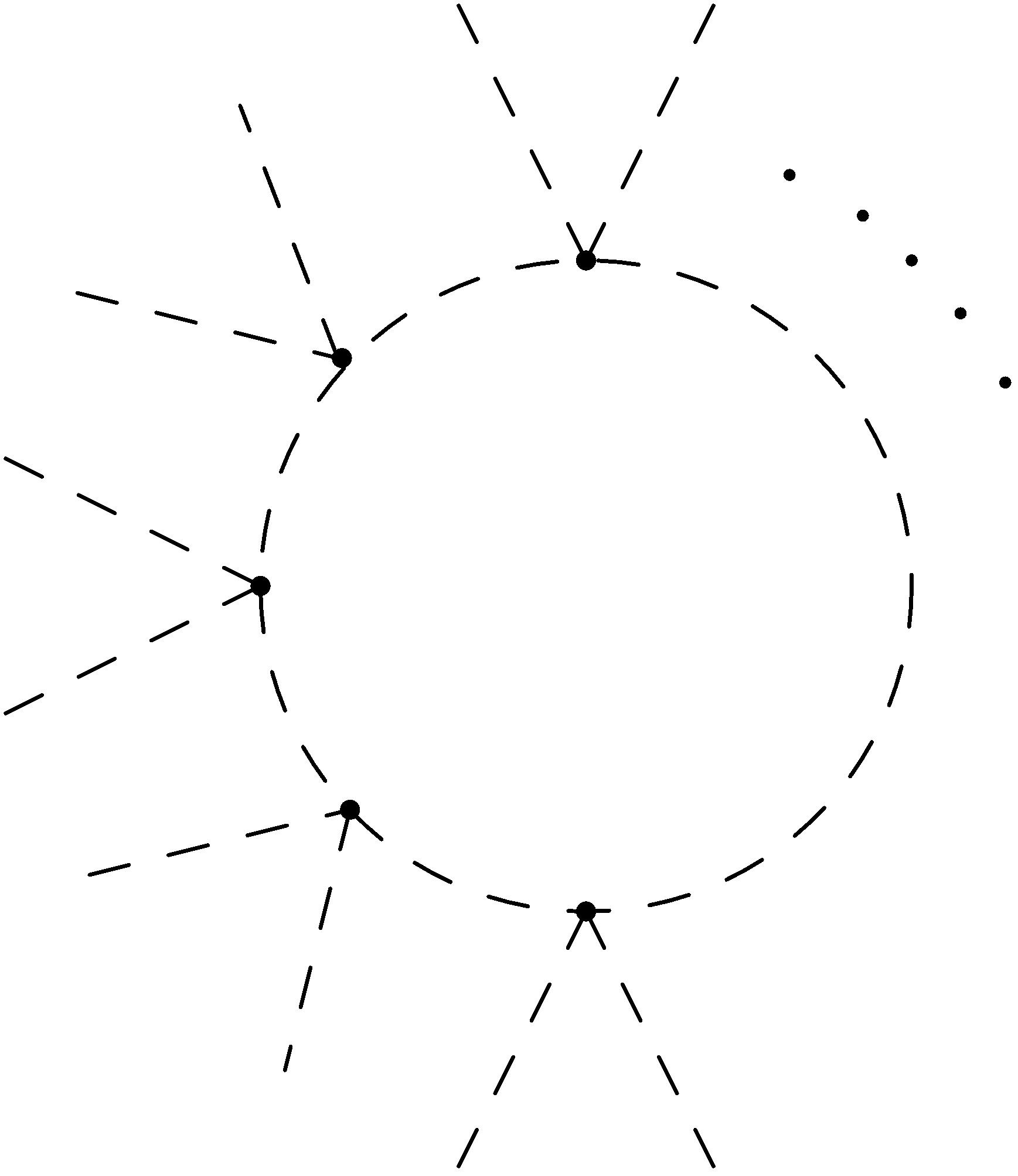
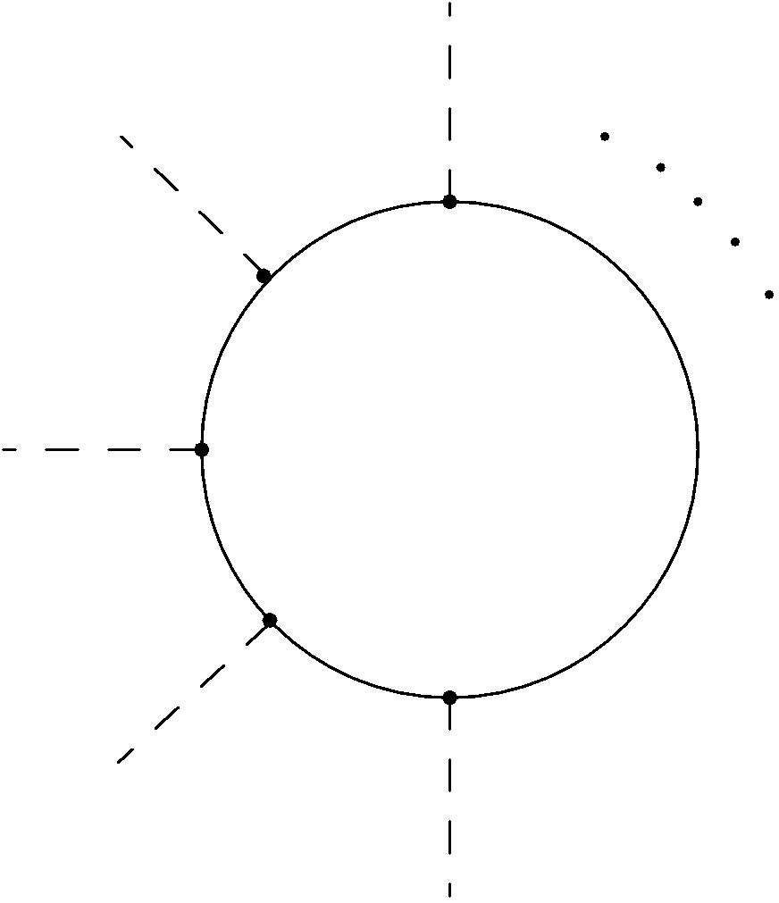
Figure 3: Diagrammatic representation for the two contributions to the RG flow equation (33) of $\hat{\lambda}_{n}$ in the DER and in the UV limit, where the rescaled Higgs quartic coupling $\hat{\lambda}_{2}$ plays a dominant role.

Thanks to Eq. (32), it is possible to encode all the rescalings from $\lambda_{n}$ for $n>2$ to $\hat{\lambda}_{n}$ in a suitable redefinition of the field invariant $\rho$. This can be achieved by defining

$$z =h^{2}\rho,$$ (36)

$$d_{z} =2+\eta_{\phi}+\eta_{h^{2}}\equiv 2+\eta_{z}.$$ (37)

By projecting the left-hand side of the above RG flow for $u(\rho)$, where Eq. (35) is substituted inside Eq. (23), onto the ansatz in Eq. (30) with $\kappa=0$ and $N_{\mathrm{p}}\to\infty$, it is possible to solve the QFP condition for all $\hat{\lambda}_{n}$. The solution is indeed

$$\hat{\lambda}_{2} =\hat{\lambda}_{2}^{\pm},$$ (38)

$$\hat{\lambda}_{n>2} =\frac{(-1)^{n}n!}{32\pi^{2}}\,\frac{(3\hat{\lambda}_{2})^{n}-12}{4-n(2+\eta_{z})},$$ (39)

and the resummation of the series has an analytic expression in terms of the hypergeometric function ${}_{2}F_{1}(a,b,c,z)$. In fact the effective potential reads

$$u(\rho) =\Bigg{[}\hat{\lambda}_{2}\frac{z^{2}}{2h^{2}}$$

$$\quad+\frac{1}{32\pi^{2}}\frac{(3\hat{\lambda}_{2}z)^{3}}{2+3\eta_{z}}\,_{2}F_{1}\left(1,\frac{2+3\eta_{z}}{2+\eta_{z}},\frac{4+4\eta_{z}}{2+\eta_{z}},-3\hat{\lambda}_{2}z\right)$$

$$\quad-\frac{3}{8\pi^{2}}\frac{z^{3}}{2+3\eta_{z}}\times$$

$$\quad\times_{2}F_{1}\left(1,\frac{2+3\eta_{z}}{2+\eta_{z}},\frac{4+4\eta_{z}}{2+\eta_{z}},-z\right)\Bigg{]}_{z=h^{2}\rho}$$ (40)

which has the property

$$\lim_{z\to 0}u^{\prime\prime}(z)=\frac{\hat{\lambda}_{2}}{h^{2}},$$ (41)

as it is clear from the chosen polynomial ansatz.

Since this solution is constructed by resummation of a local expansion for small field amplitudes, it might depart from the actual fixed-point potential at large values of $\rho$ due to nonanalytic terms. We are interested mainly in the asymptotic region $\rho\to\infty$ in the UV where $h^{2}\to 0$. However, because the QFP solution $u(\rho)$ is a function of both variables $\rho$ and $h^{2}$, there might be several such asymptotic regions, corresponding to different ways of taking the combined limit $\rho\to\infty$ and $h^{2}\to 0$. To classify these possible limits, we address the dependence of loop effects on $h^{2}$ and $\rho$. By inputting the asymptotic UV scaling of $\lambda_{2}$, the threshold functions for the bosonic and fermionic loops in Eq. (23) are functions of $\omega=3\hat{\lambda}_{2}z$ and $\omega_{1}=z$ respectively. Thus, the variable entering the threshold functions is $z$ as defined in Eq. (36). Therefore we can identify an outer region where $z\gg 1$ and an inner region where $z\ll 1$. In App. B we address in more detail this combined limit and show that it exists and is the same in both asymptotic regions, such that Eq. (40) does give a definite answer concerning the stability of the potential $u(\rho)$ for an arbitrarily small value of $h^{2}$. In fact

$$u(\rho)\mathrel{\underset{\rho\to\infty}{\scalebox{2.0}[1.0]{$\sim$}}}\frac{1}{2}\hat{\lambda}_{2}\frac{z^{2}}{h^{2}}.$$ (42)

This proves that the CEL solution corresponds to a bounded potential in the DER.

V Effective field theory analysis including thresholds

In this section we relax the restriction adopted in Sec. IV to the DER, and we account for the running of the scalar mass term. In other words, we include the possibility for a nontrivial minimum, by choosing a polynomial expansion of the scalar potential around $\rho=\kappa\neq 0$ as in Eq. (30). By projecting the left-hand side of the Eq. (23) onto this ansatz, we can derive the flow equations for the rescaled couplings $\hat{\lambda}_{n}$ as defined in Eq. (11) and Eq. (31). Similarly, also the coupling $\kappa$ may scale asymptotically as a definite power of $h^{2}$. We define

$$\hat{\kappa}=h^{2Q}\kappa,$$ (43)

where the real power $Q$ is a priori arbitrary.

Let us denote by $\beta_{n}$ the beta function of $\hat{\lambda}_{n}$, $\beta_{n}=\partial_{t}\hat{\lambda}_{n}$. In order to construct polynomial solutions of the QFP equations for the couplings $\hat{\lambda}_{n}$ and $\hat{\kappa}$, we set up the following recursive problem: we solve the equation $\beta_{\hat{\kappa}}=0$ for $\hat{\lambda}_{2}$, and $\beta_{n}=0$ for $\hat{\lambda}_{n+1}$. Upon truncating the series of equations at some $\beta_{N_{\mathrm{p}}}$, this can be achieved only if one more coupling $\hat{\lambda}_{N_{\mathrm{p}}+1}$ is retained. The result of this construction is a set of QFPs for $\hat{\lambda}_{n}$ as functions of the couplings $h^{2}$ and $\hat{\kappa}$. Also, some of the parameters $P$, $P_{n}$ and $Q$ might remain unconstrained. A defining requirement for a viable QFP solution to represent an AF trajectory is that the couplings $\hat{\lambda}_{n}$ and $\hat{\kappa}$ approach constants for $h^{2}\to 0$.

Clearly, there is some freedom in the search for scaling solutions and particularly in the recursive procedure we have described. Of course, it is likewise possible to treat another scalar coupling as a “free” parameter and to solve for $\hat{\kappa}$ in terms of some $\hat{\lambda}_{n}$. The question which coupling should meaningfully be treated as free parameter cannot be answered a priori and depends again on the precise details of the model. We choose $\hat{\lambda}_{N_{\mathrm{p}}+1}$ here to start with. For definiteness, we concentrate in this work on solutions exhibiting the property that $\hat{\lambda}_{2}\neq 0$ at the QFP (though this might be a scheme-dependent statement).

We now illustrate this process by considering $N_{\mathrm{p}}=2$; the analysis can straightforwardly be extended to any higher order. Again we adopt the approximation of setting the anomalous dimension inside the threshold functions in Eqs. (23)-(27) to zero.

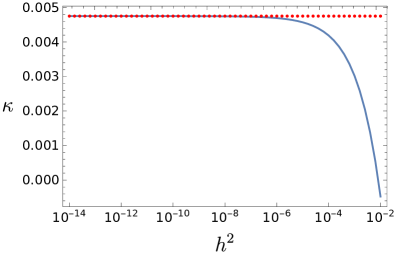
Figure 4: Effective field theory analysis including thresholds for the case $P=1/4$. We plot the full numerical solutions $\kappa\left(h^{2}\right)$ (upper panel) and $\hat{\lambda}_{2}\left(h^{2}\right)$ (lower panel) as a function of $h^{2}$ for the fixed value $\hat{\lambda}_{3}=1$ as blue solid line. The red dashed lines correspond to the leading-order constant solutions highlighted in Eq. (46) and Eq. (47).

V.1 $P\in\left(0,1/2\right)$

Because of the qualitative similarity between the flow equations of the present model and those analyzed in Refs. Gies and Zambelli (2015, 2017), we know that the finite ratio $\hat{\kappa}$ defined in Eq. (43) is actually $\kappa$ itself for $P$ being equal or smaller then $1/2$. Thus, we immediately make the ansatz $Q=0$, which turns out to be the correct solution. Indeed the leading orders in $h^{2}$ in the flow equations of the rescaled couplings are

$$\partial_{t}\hat{\lambda}_{2} =-\frac{\hat{\lambda}_{3}\,h^{2P_{3}-4P}}{16\pi^{2}}+\frac{9\hat{\lambda}_{2}^{2}\,h^{4P}}{16\pi^{2}}+\frac{\kappa\hat{\lambda}_{3}^{2}\,h^{4P_{3}-8P}}{16\pi^{2}\hat{\lambda}_{2}},$$ (44)

$$\partial_{t}\kappa =-2\kappa+\frac{3}{32\pi^{2}}+\frac{\kappa\hat{\lambda}_{3}\,h^{2P_{3}-4P}}{16\pi^{2}\hat{\lambda}_{2}}.$$ (45)

The QFP condition admits two solutions, each of them is a one parameter family of solutions. One solution corresponds to the case where the contribution coming from $\hat{\lambda}_{3}$ is subleading in Eq. (45), i.e., $P_{3}>2P$, and it reads

$$\kappa =\frac{3}{64\pi^{2}},\quad\quad\quad Q =0,$$ (46)

$$\hat{\lambda}_{2}^{2} =\frac{\hat{\lambda}_{3}}{9},\quad\quad\quad P_{3} =4P,$$ (47)

thus $\hat{\lambda}_{3}$ must be positive, but is otherwise arbitrary. In Fig. 4 it is shown how the numerical solutions for the full $h^{2}$-dependent flow equations (in the approximation detailed at the beginning of the present section) are in agreement with the leading order approximation and approach the constant values in Eq. (46) and Eq. (47) in the $h^{2}\to 0$ limit.

By contrast, the second solution corresponds to the case where the $\hat{\lambda}_{3}$ term contributes to the flow equation for $\kappa$ in the UV limit, i.e., $P_{3}=2P$. Indeed, we have that

$$\kappa =\frac{5}{64\pi^{2}},\qquad Q =0,$$ (48)

$$\hat{\lambda}_{2} =\frac{5\hat{\lambda}_{3}}{64\pi^{2}},\qquad P_{3} =2P,$$ (49)

where again the rescaled cubic scalar coupling remains a free parameter.

While the first class of solutions in Eqs. (46) and (47) had already been discovered in Refs. Gies and Zambelli (2015, 2017), the second one given by Eqs. (48) and (49) is new. These solutions were not observed in Refs. Gies and Zambelli (2015, 2017) because of simplifying approximations in the analysis of the RG equations. In particular, only linear insertions of the coupling $\lambda_{3}$ into the beta functions of lower-dimensional parameters were considered.

V.2 $P=1/2$

For the following $P\geq 1/2$ cases we confine the discussion to analytical approximations to leading order in the $h^{2}\to 0$ limit. Plots analogous to Fig. 4 with the numerical solutions capturing the full $h^{2}$ dependence of the QFP solutions would show a similar agreement between the two descriptions.

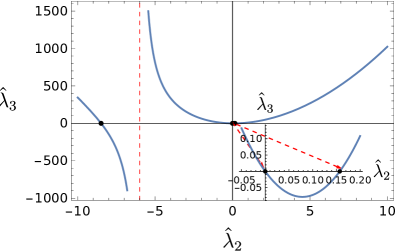
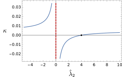
Figure 5: Effective field theory analysis including thresholds for $P=1/2$. We show the QFP solutions $\hat{\lambda}_{3}(\hat{\lambda}_{2})$ (left) and $\kappa(\hat{\lambda}_{2})$ (right) for the case $P_{3}=2$ to leading order in the $h^{2}\to 0$ limit, as expressed in Eq. (55) and Eq. (54). The left panel illustrates that for every $\hat{\lambda}_{2}\neq-6$ there is only one associated value for the free parameter $\hat{\lambda}_{3}$; the magnified inset near the origin highlights the CEL solution $\hat{\lambda}_{2}=\hat{\lambda}_{2}^{+}$ as in Eq. (16). The right panel shows that there are solutions with a positive nontrivial minimum and scalar quartic coupling only for $\hat{\lambda}_{2}>4$.

For $P=1/2$, the analysis is less straightforward and there are several possibilities. The leading $h^{2}$-contributions to the RG flow of $\hat{\lambda}_{2}$ and $\kappa$ are

$$\partial_{t}\hat{\lambda}_{2} =h^{2}\left(\frac{9\hat{\lambda}_{2}^{2}}{16\pi^{2}}+\frac{75\hat{\lambda}_{2}}{16\pi^{2}}-\frac{3}{4\pi^{2}}\right)+\frac{\kappa\hat{\lambda}_{3}^{2}\,h^{4P_{3}-4}}{16\pi^{2}\hat{\lambda}_{2}}$$

$$\quad-h^{2P_{3}-2}\left(\frac{\hat{\lambda}_{3}}{16\pi^{2}}-\frac{3\hat{\lambda}_{3}}{8\pi^{2}\hat{\lambda}_{2}}\right),$$ (50)

$$\partial_{t}\kappa =-2\kappa+\frac{3}{32\pi^{2}}-\frac{3}{8\pi^{2}\hat{\lambda}_{2}}+\frac{\kappa\hat{\lambda}_{3}\,h^{2P_{3}-2}}{16\pi^{2}\hat{\lambda}_{2}}.$$ (51)

If $P_{3}>2$ the contributions due to $\hat{\lambda}_{3}$ are negligible in the $h^{2}\to 0$ limit and we recover the CEL solution of Eq. (16). Moreover a positive (negative) solution for $\hat{\lambda}_{2}$ leads to a negative (positive) solution for $\kappa$, suggesting that the stable CEL potential possesses only the trivial minimum.

If $1<P_{3}<2$, the contribution coming from $\hat{\lambda}_{3}$ plays the dominant role in the RG flow of $\hat{\lambda}_{2}$ but is subleading for $\kappa$. The solution of the corresponding QFP equations is $\kappa=5/(64\pi^{2})$ and $\hat{\lambda}_{2}=-6$, implying that the expansion point is a nontrivial maximum. As we have assumed in our analysis that the expansion point of the Taylor series is a minimum of the potential, we reject this solution albeit it might lead to further interesting solutions if an appropriate expansion scheme is used. Thus, the only two new solutions correspond to $P_{3}=1$ and $P_{3}=2$.

In the first case, $P_{3}=1$, the solution of $\partial_{t}\hat{\lambda}_{2}=0$ is determined only by the $h^{0}$-terms. Together with Eq. (51), this leads to a $\hat{\lambda}_{2}$ which depends linearly on $\hat{\lambda}_{3}$. The solution is indeed

$$\kappa =\frac{5}{64\pi^{2}},\qquad Q =0,$$ (52)

$$\hat{\lambda}_{2} =\frac{5\hat{\lambda}_{3}}{64\pi^{2}}-6,\qquad P_{3} =1.$$ (53)

In the second case where $P_{3}=2$, the contribution given by $\hat{\lambda}_{3}$ in Eq. (51) is subleading and the corresponding QFP equation provides us $\kappa(\hat{\lambda}_{2})$. This solution can be substituted into Eq. (50) and the latter one can be solved in term of $\hat{\lambda}_{3}(\hat{\lambda}_{2})$. The corresponding solution reads

$$\kappa =\frac{3}{64\pi^{2}}\frac{\hat{\lambda}_{2}-4}{\hat{\lambda}_{2}},\qquad Q =0,$$ (54)

$$\hat{\lambda}_{3} =3\hat{\lambda}_{2}\frac{3\hat{\lambda}_{2}^{2}+25\hat{\lambda}_{2}-4}{\hat{\lambda}_{2}+6},\qquad P_{3} =2.$$ (55)

We plot this solution for $P_{3}=2$ in Fig. 5. The three black dots in the left panel highlight the three roots corresponding to $\hat{\lambda}_{3}=0$. For one of these roots, we find $\hat{\lambda}_{2}=0$ which can be discarded as the QFP value for $\kappa$ is singular in this case. The other two roots are the $\hat{\lambda}_{2}^{\pm}$ of Eq. (16). Moreover, it is clear from Eq. (54) that the condition $\hat{\lambda}_{2}>4$ has to hold to obtain a positive nontrivial minimum and at the same time a positive quadratic scalar coupling. This can also be seen in the right panel of Fig. 5.

V.3 $P\in\left(1/2,1\right)$

By following again the gauged-Higgs model discussed in Refs. Gies and Zambelli (2015, 2017) we can assume that for $P>1/2$ the nontrivial minimum goes to infinity according to some power of $h^{2}$ such that its scaling $Q$ is positive. Choosing $Q=2P-1$ as in the gauged-Higgs model turns out to be the correct scaling also for the present system. However, we prefer to be more general and consider $Q$ as an undetermined positive power in the first place. It is possible to verify that, under the assumptions that $Q>0$, $P_{3}>0$, and $P>1/2$, the only terms that can contribute to the leading parts in the RG flow for $\hat{\lambda}_{2}$ and $\hat{\kappa}$ are

$$\partial_{t}\hat{\lambda}_{2} =\frac{\hat{\lambda}_{3}^{2}\hat{\kappa}\,h^{4P_{3}-8P-2Q}}{16\pi^{2}\hat{\lambda}_{2}(1+2\hat{\lambda}_{2}\hat{\kappa}h^{4P-2Q})^{2}}-\frac{3\,h^{4-4P}}{4\pi^{2}(1+h^{2-2Q}\hat{\kappa})^{3}}$$

$$\quad-\frac{3\hat{\lambda}_{3}h^{2-8P+2\gamma}}{8\pi^{2}\xi_{2}(1+h^{2-2Q}\hat{\kappa})^{2}}+\frac{\hat{\kappa}^{2}\hat{\lambda}_{3}^{2}\,h^{4P_{3}-4Q-4P}}{4\pi^{2}(1+2h^{4P-2Q}\hat{\lambda}_{2}\hat{\kappa})^{3}}$$

$$\quad+\frac{\hat{\kappa}^{3}\hat{\lambda}_{3}^{2}\,h^{4P_{3}-6Q}}{2\pi^{2}(1+2h^{4P-2Q}\hat{\lambda}_{2}\hat{\kappa})^{4}}\hat{\lambda}_{2}(1-P),$$ (56)

$$\partial_{t}\hat{\kappa} =-2\hat{\kappa}+(Q-1)\frac{\hat{\kappa}^{4}\hat{\lambda}_{3}^{2}\,h^{4P_{3}-6Q}}{4\pi^{2}(1+2h^{4P-2Q}\hat{\lambda}_{2}\hat{\kappa})^{4}}$$

$$\quad-\frac{3\,h^{2-4P+2Q}}{8\pi^{2}\hat{\lambda}_{2}(1+h^{2-2Q}\hat{\kappa})^{2}}.$$ (57)

By analyzing all the possible combinations among the three powers $Q$, $P_{3}$ and $P$, one has to take care that the two powers of $h^{2}$ in the denominators, i.e., $2P-Q$ and $1-Q$, give different contributions to the $\beta$ functions depending on whether they are positive or negative. Moreover, we have to keep in mind that – by definition of the finite ratios – $\hat{\lambda}_{2}$ and $\hat{\kappa}$ have to approach their QFP values in the UV limit up to subleading corrections in some positive power of $h^{2}$. Among the set of all possible configurations there are only two QFP solutions. One of these corresponds to the case where the contribution arising from $\hat{\lambda}_{3}$ is subleading in Eq. (57):

$$\hat{\kappa} =\frac{3}{8\pi^{2}\hat{\lambda}_{3}},\qquad Q =2P-1,$$ (58)

$$\hat{\lambda}_{2} =-\frac{\hat{\lambda}_{3}}{2},\qquad P_{3} =2P+1,$$ (59)

where $\hat{\lambda}_{3}$ is a free parameter.

By contrast, the second solution is the one where $\hat{\lambda}_{3}$ provides a leading contribution to the flow equation for $\hat{\kappa}$. By solving the QFP condition in terms of the nontrivial minimum this solution reads

$$\hat{\lambda}_{2} =\frac{-2\pm\sqrt{2P-1}}{2(5-2P)\hat{\kappa}},\qquad Q =2P,$$ (60)

$$\hat{\lambda}_{3}^{2} =\frac{8\pi^{2}(1+2\hat{\kappa}\hat{\lambda}_{2})^{4}}{(2P-1)\hat{\kappa}^{3}},\quad P_{3} =3P.$$ (61)

We can therefore deduce that there are no reliable solutions that fulfill our assumptions for $P\in(1/2,1)$ because it is not possible to simultaneously satisfy the condition that both the Higgs quartic coupling and the nontrivial expansion point $\kappa$ are positive.

V.4 $P=1$

Starting from Eq. (56) and Eq. (57), it is possible to prove that for $P=1$ there are again two QFP solutions corresponding to different combinations for the two left powers $P_{3}$ and $Q$. One solution is

$$\hat{\lambda}_{3} =\frac{3}{8\pi^{2}\hat{\kappa}(1+\hat{\kappa})^{3}},\qquad P_{3} =3,$$ (62)

$$\hat{\lambda}_{2} =-\frac{3}{16\pi^{2}\hat{\kappa}(1+\hat{\kappa})^{2}},\qquad Q =1,$$ (63)

whereas the second one reads

$$\hat{\lambda}_{3}^{2} =\frac{128\pi^{2}}{81\hat{\kappa}^{3}},\qquad P_{3} =3,$$ (64)

$$\hat{\lambda}_{2} =-\frac{1}{6\hat{\kappa}},\qquad Q =2.$$ (65)

We observe once more that there are no solutions with positive $\kappa$ and a positive scalar quartic coupling such that we expand the potential around a nonvanishing vacuum expectation value of the scalar field.

In App. C we complete the EFT analysis of the present section, by discussing $P>1$. Also in this case we conclude that all the QFP solutions we observe have either $\hat{\lambda}_{2}$ or $\hat{\kappa}$ negative.

VI Full effective potential in the $\phi^{4}$-dominance approximation

So far, we have projected the RG flow of the potential onto a polynomial basis and studied only the running of the various coefficients. Now, we investigate the functional RG flow of an arbitrary scalar potential which also includes nonpolynomial structures Coleman and Weinberg (1973); Jackiw (1974). The latter is obtained by performing a one-loop computation with field-dependent thresholds. The loop integrals are evaluated by using the piece-wise linear regulator Litim (2000, 2001). To simplify the discussion, we neglect the possible appearance of higher-dimensional couplings in the other $\beta$ functions and anomalous dimensions, and ignore contributions which would be present only in the SSB regime. Thus in the following, we use Eq. (23) together with Eqs. (2), (3), and the one-loop value for the anomalous dimension of the scalar field given in Eq. (10).

We pursue the identification of AF trajectories in the space of all flows described by integration of Eq. (23) for generic boundary conditions. We already know from the previous sections that AF solutions can in fact be constructed by simply looking for QFPs of the flow of $h^{2}$-rescaled interactions. To implement this condition in a functional set-up, we define a new field variable and its potential

$$\begin{split}x&=h^{2P}\rho,\quad\quad f(x)=u(\rho).\end{split}$$ (66)

We denote the minimum by $x_{0}$ and the couplings by $\xi_{n}$,

$$\begin{split}f^{\prime}(x_{0})&=0,\qquad f^{(n)}(x_{0})=\xi_{n}.\end{split}$$ (67)

The arbitrary rescaling power $P$ is chosen to be that of Eq. (11) so that $\xi_{2}=\hat{\lambda}_{2}$, because we specifically look for QFPs where $\hat{\lambda}_{2}\neq 0$. It might happen that at a QFP $x_{0}\neq\hat{\kappa}$, and $\xi_{n}\neq\hat{\lambda}_{n}$ for $n>2$, such that solutions of the equation $\partial_{t}f(x)=0$ might differ from the actual scaling solutions. Thus, the rescaling of Eq. (66) is expected to be useful as long as the quartic scalar coupling is the leading term in the approach of the scalar potential towards flatness.

As a first-level approximation, we consider an intermediate step between the polynomial and the functional approaches, which is based on the expectation that the marginal quartic coupling plays a dominant role in the UV. Therefore, we assume that the contribution coming from the scalar fluctuations is dominated by a plain quartic interaction. More precisely, we use $\omega=3\lambda_{2}\rho$ on the right-hand side of Eq. (23), but we consider the scalar potential as an unknown arbitrary function in the scaling term and on the left-hand side of the flow equation itself. This leads to the following flow equation

$$\partial_{t}f(x) =-4f(x)+d_{x}xf^{\prime}(x)+\frac{1}{32\pi^{2}}\,\frac{1}{1+3\xi_{2}h^{2P}x}$$

$$\quad-\frac{3}{8\pi^{2}}\,\frac{1}{1+h^{2-2P}x}.$$ (68)

where

$$d_{x}=2+\eta_{\phi}+P\eta_{h^{2}}\equiv 2+\eta_{x}\ .$$ (69)

The anomalous dimension $\eta_{x}$ of the rescaled field invariant $x$ includes also the introduced anomalous dimension of the Yukawa coupling $\eta_{h^{2}}$ defined in Eq. (12).

By setting the left-hand side to zero, we get a first-order linear ordinary differential equation that can be solved analytically for generic $P$ and its QFP solution is

$$f(x) =\frac{1}{128\pi^{2}}\,_{2}F_{1}\left(1,-\frac{4}{2+\eta_{x}},\frac{-2+\eta_{x}}{2+\eta_{x}},-3\xi_{2}h^{2P}x\right)$$

$$\quad-\frac{3}{32\pi^{2}}\,_{2}F_{1}\left(1,-\frac{4}{2+\eta_{x}},\frac{-2+\eta_{x}}{2+\eta_{x}},-h^{2-2P}x\right)$$

$$\quad+C_{\mathrm{f}}\,x^{\frac{4}{2+\eta_{x}}},$$ (70)

where the term proportional to the free integration constant $C_{\mathrm{f}}$ is the homogeneous solution of Eq. (68) while the Gauß hypergeometric functions are particular solutions obtained by integrating the non-homogeneous part.

For $C_{\mathrm{f}}=0$ we can straightforwardly impose the consistency condition $f^{\prime\prime}(0)=\xi_{2}$. Instead, for any nonvanishing $C_{\mathrm{f}}$, the QFP potential behaves as a nonrational power of $x$ at the origin. Its second order derivative is not defined at the origin as long as $\eta_{x}>0$ which is generically the case for a potential in the symmetric regime. This problem might be avoided if there is at least one nontrivial minimum $x_{0}$, in the spirit of the Coleman-Weinberg mechanism Coleman and Weinberg (1973). In fact, we can impose $f^{\prime\prime}(x_{0})=\xi_{2}$ for this xcase.

As a first analysis, we want to understand the asymptotic properties of the full $h^{2}$-dependent solution $f(x)$. Specifically, we want to identify parameter ranges for $C_{\mathrm{f}}$ and $\xi_{2}$ for which the potential is bounded from below. To this end, we focus on the asymptotic behavior of the solution, $x\to+\infty$. In particular, we are interested in the UV regime where $h^{2}\to 0$. Since the QFP potential $f(x)$ for given $C_{\mathrm{f}}$, which might also depend on $h^{2}$, is a function of the two variables $x$ and $h^{2}$, we have to take the limit process with care to investigate the asymptotic behavior of $f$ in the deep UV.

In order to address the asymptotic behavior of the QFP potential in a systematic way, we analyze the flow for fixed arguments,

$$z_{\mathrm{B}} =3\xi_{2}h^{2P}x,\qquad z_{\mathrm{F}}=h^{2(1-P)}x,$$ (71)

of the hypergeometric functions. For small enough $h^{2}$ and $P\gtrless 1/2$, we have $z_{\mathrm{F}}\gtrless z_{\mathrm{B}}$. Thus, one can divide the interval $x\in[0,\infty)$ into three distinct domains. Suppose $z_{\mathrm{F}}<z_{\mathrm{B}}$, then we define the $h$-dependent boundary $x_{1}(h)$ of an inner interval $x\in[0,x_{1})$ by requiring $z_{\mathrm{B}}=1$ and the boundary $x_{2}(h)$ of an outer interval $(x_{2},\infty)$ by $z_{\mathrm{F}}=1$ for fixed $P$ and $\xi_{2}$. For $z_{\mathrm{F}}>z_{\mathrm{B}}$, the requirement $z_{\mathrm{B}}=1$ and $z_{\mathrm{F}}=1$ will define $x_{2}$ and $x_{1}$, respectively. In case $P<1$, the two boundaries $x_{1}$ and $x_{2}$ grow towards larger values and always fulfill $x_{2}>x_{1}$ when we send $h\to 0$.

Approximating the hypergeometric functions for small but fixed arguments $z_{\mathrm{B}/\mathrm{F}}\ll 1$, we obtain a valid approximation of the potential in the first interval as this also implies $x\ll x_{1}$. Thus, we are able to reliably check the asymptotic behavior by first performing the limit $h\to 0$ and afterwards $x\to\infty$ in this region. In case the hypergeometric functions shall be investigated for large arguments, we have to perform first the limit $x\to\infty$ before sending $h\to 0$ to investigate the asymptotic behavior such that one stays in the outer interval as only there the results can be trusted for the used approximations. Further details can be found in App. B.2. The rescaled potential $f(x)$ turns out to be stable in the deep UV for both regimes, and the two asymptotic behaviors are in agreement.

VI.1 Large-field behavior

For finite values of $h^{2}$, we can investigate the asymptotic behavior in the interval $(x_{2},\infty)$ by expanding the QFP potential in Eq. (70) around $x=\infty$. The analytic expansion yields

$$f(x)=C_{\mathrm{f},\infty}\,x^{\frac{4}{2+\eta_{x}}}+\mathcal{O}(x^{-1}),$$ (72)

where the asymptotic coefficient in front of the scaling term depends on the different parameters characterizing the RG trajectory $C_{\mathrm{f},\infty}(C_{\mathrm{f}},\xi_{2},h^{2},P)$. The full expression is given in App. B.2, cf. Eq. (127). We investigate its $h^{2}$ dependence in the deep UV by an expansion at vanishing Yukawa coupling. This yields a scaling $C_{\mathrm{f},\infty}\,{\sim}\,h^{-2(1-2P)}$ for $P\in(0,1/2)$ and $C_{\mathrm{f},\infty}\,{\sim}\,h^{-2(2P-1)}$ for $P\in(1/2,1)$ for fixed $C_{\mathrm{f}}$. We call $\hat{C}_{\mathrm{f},\infty}$ the corresponding finite ratio. For the sake of clarity, it is therefore useful to define a new variable

$$\hat{C}_{\mathrm{f}}=\left\{\begin{aligned} &h^{2(1-2P)}C_{\mathrm{f}}&&\text{if}\quad P\in(0,1/2),\\ &C_{\mathrm{f}}&&\text{if}\quad P=1/2,\\ &h^{2(2P-1)}C_{\mathrm{f}}&&\text{if}\quad P\in(1/2,1).\end{aligned}\right.$$ (73)

From this rescaling we obtain that the asymptotic coefficient has to be

$$\hat{C}_{\mathrm{f},\infty}=\left\{\begin{aligned} &\hat{C}_{\mathrm{f}}-\frac{9}{64\pi^{2}\hat{\eta}_{x}}\xi_{2}^{2}&&\text{if}\quad P\in(0,1/2),\\ &C_{\mathrm{f}}-\frac{9\xi_{2}^{2}-12}{64\pi^{2}\hat{\eta}_{x}}&&\text{if}\quad P=1/2,\\ &\hat{C}_{\mathrm{f}}+\frac{3}{16\pi^{2}\hat{\eta}_{x}}&&\text{if}\quad P\in(1/2,1),\end{aligned}\right.$$ (74)

in leading order in $h^{2}$ where $\hat{\eta}_{x}=\eta_{x}/h^{2}$. The locus of points that satisfies the condition $\hat{C}_{\mathrm{f},\infty}=0$ for $P\leq 1/2$ are plotted in Fig. 6 by black lines. They characterize the transition from the region in the $(\hat{C}_{\mathrm{f}},\xi_{2})$ plane where the potential is bounded from below (right side) to the region where the potential is unbounded (left side).

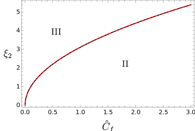
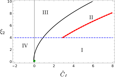
I            II            III            IV  

Figure 6: Stability properties of the effective potential $f(x)$, see Eq. (70), for $P\in(0,1/2)$ (upper left) and $P=1/2$ (upper right). The two black lines separate the left-hand side regions where the potential is unbounded from below from the right-hand side regions where it is bounded, and in the $h^{2}\to 0$ limit. Their equations are obtained imposing the condition $\hat{C}_{\mathrm{f},\infty}=0$ in Eq. (74). Sketches of the potential shapes in the different regions are given in the lower panels. Upper right: the blue dashed line $\xi_{2}=4$ identifies the locus of points where $f^{\prime}(0)=0$. For $\xi_{2}<4$, the potential has an unstable minimum in region IV. It is monotonically increasing to $+\infty$ in region I. For $\xi_{2}>4$, $f(x)$ has a stable minimum in region II. It is monotonically decreasing to $-\infty$ in region III. The green point $\{0,\hat{\lambda}_{2}^{+}\}$ highlights the CEL solution, see Eq. (16), being regular at $x=0$. The red dashed line in region II shows the one parameter family of new solutions satisfying the consistency condition $f^{\prime\prime}(x_{0})=\xi_{2}$, as expressed in Eq. (85). Upper left: only the regions of type II and III are present.

VI.2 Small-field behavior and the CEL solution

Next, we study the properties of the solution $f(x)$ for small arguments $x\ll 1$. This is relevant to address both the $x\to 0$ limit at fixed $h^{2}$, and also to inspect the large field asymptotics for $P<1$ in the limit where $h^{2}\to 0$ and $x\to+\infty$ at $z_{\mathrm{B}/\mathrm{F}}\ll 1$. For this purpose, we start from the expansion of the QFP potential $f(x)$ for small $x$, which can be found in App. B.2, cf. Eq. (131). The Gauß  hypergeometric functions are analytical for small $x$, but the scaling term is not, due to the nonrational power of $x$. The first derivative at the origin is

$$f^{\prime}(0)=\frac{12-3h^{2(2P-1)}\xi_{2}}{32\pi^{2}(2-\eta_{x})}h^{2(1-P)},$$ (75)

thus by keeping the leading order in $h^{2}$ we have

$$f^{\prime}(0)=\left\{\begin{aligned} &-\frac{3\,\xi_{2}}{64\pi^{2}}h^{2P}&&\text{if}\quad P\in(0,1/2),\\ &\frac{12-3\xi_{2}}{64\pi^{2}}\,h&&\text{if}\quad P=1/2,\\ &\frac{3}{16\pi^{2}}\,h^{2(1-P)}&&\text{if}\quad P\in(1/2,1).\end{aligned}\right.$$ (76)

Thus, we observe that $f^{\prime}(0)$ is negative for $P<1/2$ and $\xi_{2}>0$ while it is always positive for $P>1/2$.

For $P=1/2$, the first derivative at the origin changes sign at $\xi_{2}=4$. In this case, we find that the two lines $C_{\mathrm{f},\infty}=0$ and $\xi_{2}=4$ divide the ($C_{\mathrm{f},\infty},\xi_{2}$) plane in four regions with different qualitative behavior for $f(x)$, as represented in the right panel of Fig. 6 with solid black line and dashed blue line respectively. In region II the QFP potential is bounded from below and has a nontrivial stable minimum. In region IV the potential has a nontrivial maximum but is unbounded from below. Instead in regions I and III the function $f(x)$ is monotonically increasing towards $+\infty$ and decreasing to $-\infty$, respectively. For $P<1/2$, there are only regions of type II and III.

In region I, where the potential is bounded from below and its minimum is located at the origin, we have to check as to whether it is possible to impose the consistency condition $f^{\prime\prime}(0)=\xi_{2}$. The answer is positive if we remove the log-type singularity in the second derivative at the origin by requiring $C_{\mathrm{f}}=0$. With this choice, we obtain

$$\xi_{2}=3h^{2(1-2P)}\,\frac{4-3h^{4(2P-1)}\xi_{2}^{2}}{32\pi^{2}\hat{\eta}_{x}} \text{if}\quad C_{\mathrm{f}}=0$$ (77)

where the rescaled quartic scalar coupling $\xi_{2}$, by definition, must be finite in the $h^{2}\to 0$ limit. Therefore the only possible solution is

$$\xi_{2}=\hat{\lambda}_{2}^{\pm},\quad P=\frac{1}{2},$$ (78)

that is precisely the CEL solution described in Sec. II. The positive root $\hat{\lambda}_{2}^{+}$ is highlighted by a a green dot in the right panel of Fig. 6.

Having constructed a full effective potential for the CEL solution, we can ask whether this is stable for large field amplitudes and how it is related to the $u(\rho)$ of Eq. (40). As shown in App. B.3, we have

$$\lim_{d_{x}\to d_{z}}f(x)=u(\rho)+\frac{12-3\xi_{2}}{32\pi^{2}(2-\eta_{z})}hx,$$ (79)

where an irrelevant additive constant has been neglected. Therefore the full solution $f(x)$ includes all the information about $u(\rho)$ plus a linear term that was discarded in Sec. IV by the definition of the DER. Furthermore, Eq. (72) and Eq. (74) apply to all values of $C_{\mathrm{f}}$, thus by choosing $P=1/2$ and $C_{\mathrm{f}}=0$ in these equations, and specifying the QFP value of $\xi_{2}$, we deduce that the asymptotic behavior for the CEL potential is

$$f(x)\mathrel{\underset{x\to\infty}{\scalebox{2.0}[1.0]{$\sim$}}}\frac{\xi_{2}}{2}x^{2}.$$ (80)

Thus, we conclude that the CEL solution is stable for arbitrary small values of the Yukawa coupling.

VI.3 New solutions with a nontrivial minimum

Within region II, the potential is stable and has a nontrivial minimum. Here, we demand the consistency condition to hold at the minimum, $f^{\prime\prime}(x_{0})=\xi_{2}$. To simplify the discussion we adopt the same small-field expansion discussed above, which corresponds to neglecting subleading powers of $x_{0}$, for small values of the vacuum expectation value. The defining condition for the minimum, $f^{\prime}(x_{0})=0$, gprovides an expression for $C_{\mathrm{f}}$ as a function of $x_{0}$, $h^{2}$ and $\xi_{2}$ which is

$$C_{\mathrm{f}}=x_{0}^{\frac{\eta_{x}-2}{2+\eta_{x}}}\frac{h^{2(1-P)}(2+\eta_{x})}{128\pi^{2}(2-\eta_{x})}\left[3\xi_{2}h^{2(2P-1)}-12\right].$$ (81)

The second derivative of the potential in $x_{0}$ is thus

$$f^{\prime\prime}(x_{0})=\frac{3\xi_{2}h^{2(2P-1)}-12}{32\pi^{2}(2+\eta_{x})x_{0}}h^{2(1-P)},$$ (82)

which, together with $f^{\prime\prime}(x_{0})=\xi_{2}$, provides us with an expression for the nontrivial minimum as a function of $h^{2}$ and $\xi_{2}$

$$x_{0}=\frac{3\xi_{2}h^{2(2P-1)}-12}{32\pi^{2}\xi_{2}(2+\eta_{x})}h^{2(1-P)}.$$ (83)

Different powers of $P$ lead to different leading behaviors in $h^{2}$ for the latter expression. These can be summarized in the following way

$$x_{0}=\left\{\begin{aligned} &\frac{3}{64\pi^{2}}h^{2P}&&\text{if}\quad P\in(0,1/2),\\ &\frac{3\xi_{2}-12}{64\pi^{2}\xi_{2}}h&&\text{if}\quad P=1/2,\\ &-\frac{3}{16\pi^{2}\xi_{2}}h^{2(1-P)}&&\text{if}\quad P\in(1/2,1).\end{aligned}\right.$$ (84)

These results are in agreement with the EFT analysis including thresholds presented in Sec. V. In fact Eqs. (46), (54), and (58) are identical to those in Eq. (84), recalling that $x_{0}=h^{2P}\kappa$.

Moreover, we can substitute the expression for the minimum $x_{0}(\xi_{2},h^{2})$ inside the parametrization for $C_{\mathrm{f}}$ in Eq. (81) for $P=1/2$. Considering the leading order in $h^{2}$, we find

$$C_{\mathrm{f}} =\frac{9\xi_{2}^{2}-12}{64\pi^{2}\hat{\eta}_{x}}+\frac{\xi_{2}}{2}\quad\text{for}\quad P=\frac{1}{2},$$ (85)

that describes a one-parameter family of QFP solutions satisfying the consistency condition at the nontrivial minimum, i.e., $f^{\prime\prime}(x_{0})=\xi_{2}$. These solutions are represented in the right panel of Fig. 6 as a red dashed line laying in Reg. II. The asymptotic behavior for the latter solutions is obtained by plugging Eq. (85) into Eq. (74). It turns out that these solutions obey the same asymptotic behavior as the CEL solution which is given by a quadratic function in $x$,

$$f(x)\mathrel{\underset{x\to\infty}{\scalebox{2.0}[1.0]{$\sim$}}}\frac{\xi_{2}}{2}x^{2}\quad\text{for}\quad P=\frac{1}{2}.$$ (86)

Also for $P<1/2$ it is possible to find a parametrization $C_{\mathrm{f}}(\xi_{2})$ for the QFP solutions with a nontrivial minimum satisfying the consistency condition in $x_{0}$. Its leading order contribution in $h^{2}$ reads

$$\hat{C}_{\mathrm{f}}=\frac{9\,\xi_{2}^{2}}{64\pi^{2}\,\hat{\eta}_{x}}\quad\text{for}\quad P\in(0,1/2),$$ (87)

and coincides exactly with the solution to the condition $\hat{C}_{\mathrm{f},\infty}=0$. Thus, we find the asymptotic behavior

$$f(x)\mathrel{\underset{x\to\infty}{\scalebox{2.0}[1.0]{$\sim$}}}0\quad\text{for}\quad P\in(0,1/2).$$ (88)

Therefore, the QFP solutions for $P<1/2$ are asymptotically flat.

Along these two families of QFP solutions for $P\leq 1/2$, it is interesting to evaluate the rescaled cubic coupling at $x_{0}$. It is given by the third derivative of the homogenous scaling part with respect to $x$ which reads

$$f^{\prime\prime\prime}(x_{0})=-C_{\mathrm{f}}\frac{8\eta_{x}(2-\eta_{x})}{(2+\eta_{x})^{3}}x_{0}^{-\frac{2+3\eta_{x}}{2+\eta_{x}}}.$$ (89)

By inserting $x_{0}(\xi_{2},h^{2})$ and $C_{\mathrm{f}}(\xi_{2})$, the leading contribution in $h^{2}$ is given by

$$\xi_{3}=\left\{\begin{aligned} &-6\xi_{2}^{2}h^{2P}&&\text{if}\quad P\in(0,1/2),\\ &-2\xi_{2}h\,\frac{9\xi_{2}^{2}+32\pi^{2}\hat{\eta}_{x}\xi_{2}-12}{3\xi_{2}-12}&&\text{if}\quad P=1/2.\end{aligned}\right.$$ (90)

From the definitions (31) and (67), we deduce that the transformation between the rescaled cubic coupling for $f(x)$ and the finite ratio $\hat{\lambda}_{3}$ is

$$\xi_{3}=\hat{\lambda}_{3}h^{2(P_{3}-3P)}.$$ (91)

From Eq. (90) we can conclude that $P_{3}=2$ for $P=1/2$ and $P_{3}=4P$ for $P\in(0,1/2)$. This $h^{2}$-dependent behavior is in agreement with the EFT analysis including thresholds described in Sec. V. However, the expression for the finite ratio $\hat{\lambda}_{3}$ is different, since we are treating the threshold functions in the $\phi^{4}$-dominance approximation in this section.

Finally, let us summarize once more the results of the fixed-point potential analysis for $f(x)$ and for general $P<1$. Starting from a pure quartic scalar interaction for the potential given by $\lambda_{2}\rho^{2}/2=\xi_{2}x^{2}/{2}$ with a trivial minimum at the origin, we obtain a QFP potential of the same type and with the required property $f^{\prime\prime}(0)=\xi_{2}$ only for the particular choice for the parameters $\{P,C_{\mathrm{f}},\xi_{2}\}=\{1/2,0,\hat{\lambda}_{2}^{\pm}\}$. This is the CEL solution. We argued that it is stable with a well defined asymptotic behavior in the combined limit $x\to\infty$ and $h^{2}\to 0$. In addition for $P\leq 1/2$, we discovered in the $(\hat{C}_{\mathrm{f}},\xi_{2})$ plane the existence of a one-parameter family of new solutions. Despite the presence of a log-type singularity at the origin, these solutions have a nontrivial minimum $x_{0}$ which satisfies the consistency condition $f^{\prime\prime}(x_{0})=\xi_{2}$. For $P=1/2$ these new solutions are stable and present the same quadratic asymptotic behavior as for the CEL solution. For $P<1/2$, the QFP potential becomes asymptotically flat in the combined limit $x\to\infty$ and $h^{2}\to 0$, because $\hat{C}_{\mathrm{f},\infty}=0$.

VII Full effective potential in the weak-coupling expansion

Let us discuss yet another analytic functional approximation, obtained by expanding the full functional equation for the rescaled potential $f(x)$ in powers of $h^{2}$. The one-loop flow equation for $f(x)$ takes the form

$$\partial_{t}f=-4f+d_{x}xf^{\prime}+\frac{1}{32\pi^{2}}\frac{1}{1+\omega_{f}}-\frac{N_{\mathrm{c}}d_{\gamma}}{32\pi^{2}}\frac{1}{1+\omega_{1f}},\qquad$$ (92)

where we have chosen again the piecewise linear regulator for the evaluation of the threshold functions $l_{0}^{(\mathrm{B}/\mathrm{F})}$, as in Eq. (23), which parametrize the result of the boson/fermion loop integrals. Here, $d_{x}$ is the same as in Eq. (69) and represents the quantum dimension of $x$. The arguments $\omega_{f}$ and $\omega_{1f}$, defined as

$$\begin{split}\omega_{f}&=h^{2P}\left(f^{\prime}+2xf^{\prime\prime}\right),\qquad\omega_{1f}&=h^{2-2P}x,\end{split}$$ (93)

are related to the scalar and Yukawa vertices, respectively.

The dimension of the rescaled field $d_{x}$ depends on $\eta_{\phi}$ and $\eta_{h^{2}}$ and thus is of order $h^{2}$, cf. Eq. (10) and Eq. (13). Therefore, they can be neglected for $P<1$ and at leading order in $h^{2}$ the flow equation can be written as

$$\beta_{f}=\left[\beta_{f}\right]_{h^{2}\to 0}+\delta\beta_{f},$$ (94)

where the first term is just the $\beta$-function in the limit $h^{2}\to 0$ and the second one can be derived from the expansion of the bosonic and fermionic loops. An $h^{2}$-independent contribution from the quantum fluctuations is present only for $P=1$, and equals the fermion loop. Therefore in $d=4$ one has

$$\left[\beta_{f}\right]_{h^{2}\to 0}=\begin{cases}-4f+2xf^{\prime},\quad&\text{$P<1$,}\\ -4f+2xf^{\prime}-\frac{N_{\mathrm{c}}d_{\gamma}}{32\pi^{2}}\frac{1}{1+x},\quad&\text{$P=1$.}\end{cases}\qquad$$ (95)

For $P<1$ the zeroth order in $h^{2}$ is trivial since no quantum fluctuations are retained. On the other hand for $P=1$, the properties of the QFP solutions depend on the current choice of the regulator. Let us now discuss all interesting cases, for $P\leq 1$. For the case $P>1$, we demonstrate in App. C that no reliable solution can be constructed which is compatible with our assumptions and approximations.

VII.1 $P\in(0,1/2)$

In this case only the scalar loop contributes to the first order correction to $\beta_{f}$. The scalar vertices scale like $h^{2P}$. Therefore $\delta\beta_{f}$ can be approximated by the linear term of a Taylor expansion of the scalar threshold function at vanishing argument, reading

$$\delta\beta_{f}=-\frac{1}{32\pi^{2}}\,h^{2P}(f^{\prime}+2xf^{\prime\prime}).$$ (96)

Upon inclusion of this leading order correction, the flow equation now becomes a second order ODE that can be solved analytically. We find two linearly independent solutions. The first is given by the following polynomial

$$f(x)=c\left(x^{2}-\frac{3}{32\pi^{2}}h^{2P}x\right).$$ (97)

where $c$ is an integration constant. The second solution grows exponentially for large field amplitudes. However, we are only interested in solutions that obey power-like scaling for $x\to\infty$, since in this case a scalar product can be defined on the space of eigenperturbations of these solutions Morris (1996); O’Dwyer and Osborn (2008); Bridle and Morris (2016). Thus, we set the second integration constant to zero.

Clearly, the solution in Eq. (97) is easily translated into the polynomial language of Sec. V, by identifying

$$\begin{aligned} \xi_{2}&=2c,\\ x_{0}&=\frac{3}{64\pi^{2}}h^{2P}.\end{aligned}$$ (98)

which agrees with Eq. (46) and Eq. (47).

VII.2 $P=1/2$

For $P=1/2$, both the scalar and the fermion loops contribute to the first correction of $\beta_{f}$ that is

$$\delta\beta_{f}=-\frac{1}{32\pi^{2}}h(f^{\prime}+2xf^{\prime\prime})+\frac{1}{32\pi^{2}}N_{\mathrm{c}}d_{\gamma}hx.$$ (99)

The QFP equation is again a second order ODE whose analytic solution will have two integration constants. Again, we discard the solution which scales exponentially for large $x$ by setting the corresponding integration constant to zero. The remaining solution is a quadratic polynomial that has a free quartic coupling $\xi_{2}$ and a minimum at

$$x_{0}=h\frac{3\xi_{2}-N_{\mathrm{c}}d_{\gamma}}{64\pi^{2}\xi_{2}}.$$ (100)

By setting $N_{\mathrm{c}}=3$ and working with an irreducible representation of the Clifford algebra in $d=4$, i.e., $d_{\gamma}=4$, one recovers the result of Sec. V.2 for $P_{3}>1$. As in that case, the nontrivial minimum only exists if $\xi_{2}>4$. The straightforward generalization of this requirement reads

$$\xi_{2}>\frac{N_{\mathrm{c}}d_{\gamma}}{3}$$ (101)

for a generic field content.

VII.3 $P\in(1/2,1)$

In this case only the fermion loop contributes to the first correction of $\beta_{f}$ and is given by

$$\delta\beta_{f}=\frac{1}{32\pi^{2}}N_{\mathrm{c}}d_{\gamma}h^{2(1-P)}x.$$ (102)

The differential equation remains a first order ODE and its analytical solution is

$$f(x)=\frac{\xi_{2}}{2}x^{2}+\frac{1}{64\pi^{2}}N_{\mathrm{c}}d_{\gamma}h^{2(1-P)}x,$$ (103)

where $\xi_{2}$ is an arbitrary integration constant. For any color number or representation of the Clifford algebra, the potential exhibits only the trivial minimum at vanishing field amplitude and thus the QFP solution is in the symmetric regime. In fact the corresponding nontrivial minimum

$$x_{0}=-\frac{N_{\mathrm{c}}d_{\gamma}}{64\pi^{2}\xi_{2}}h^{2(1-P)},$$ (104)

would be negative for any positive $\xi_{2}$. This is again in agreement with the EFT analysis, cf. Eq. (58) and Eq. (59).

For all values of $P<1$ in the present approximation, we have obtained QFP solutions which are analytic in $x$. In Sec. V, this was implemented by construction, since we have projected the functional flow equation onto a polynomial ansatz. In the present analysis, this happens because the contributions to $\beta_{f}$ producing non-analyticities are accompanied by subleading powers of $h^{2}$ for $P<1$. Indeed, both the anomalous dimension of $x$ and contributions from the loops proportional to $x^{2}$ would produce a logarithmic singularity of $f^{\prime\prime}(x)$ at $x=0$ for any $h^{2}\neq 0$, as discussed in Sec. VI.2, see also below. Knowing about the presence of this singularity for any $P$ for $h^{2}\neq 0$, we can accept the previous solutions only if $x_{0}>0$, which appears to be impossible for $P\in(1/2,1)$.

VII.4 $P=1$

As shown in Eq. (95), already the zeroth order in $h^{2}$ accounts for nontrivial dynamical effects for $P=1$. The corresponding QFP solution for the piecewise linear regulator is

$$f(x)=c\,x^{2}+\frac{N_{\mathrm{c}}d_{\gamma}}{64\pi^{2}}\left(x+x^{2}\log\frac{x}{1+x}\right).$$ (105)

The second derivative of this potential has a log-type singularity at the origin. We expect that this feature survives also in the full $h^{2}$-dependent solution, as addressed in the next section.

The freedom in the choice of the parameter $c$ allows to construct physical QFP solutions, that avoid the divergence at small fields by developing a nontrivial minimum. The defining equation $f^{\prime}(x_{0})=0$ for this minimum, where $f$ is given by Eq. (105), can straightforwardly be solved for $c$ in terms of $x_{0}$. From the point of view where the latter is the free parameter labeling the QFP solutions, the natural question then is as to whether it can be chosen such that $f^{\prime\prime}(x_{0})=\xi_{2}$ is positive and finite for $h^{2}\to 0$. The answer is negative, since the piecewise linear regulator gives

$$\xi_{2}=-\frac{N_{\mathrm{c}}d_{\gamma}}{64\pi^{2}x_{0}(1+x_{0})^{2}},$$ (106)

which is in agreement with Eq. (63).

VIII Numerical solutions

In this section, we test our previous analytical results by integrating numerically the full one-loop nonlinear flow equation for $f(x)$ as in Eq. (92), where we have computed the threshold functions $l_{0}^{\mathrm{B}/\mathrm{F}}$ in Eq. (23) by choosing the piece-wise linear regulator. We make a further approximation evaluating the anomalous dimensions $\eta_{\phi}$, $\eta_{\psi}$ and $\eta_{h^{2}}$ in the DER, leading to the expressions in Eqs. (10) , (13) and (28). We are moreover interested in the $P=1/2$ case characterized by the existence of the CEL solution, regular at the origin, and a family of new QFP potentials, singular in $x=0$ but featuring a nontrivial minimum $x_{0}\neq 0$. To address this numerical issue we exploit two different methods. First, we study the global behavior of the CEL solution using pseudo-spectral methods. And second, we corroborate the existence of the new QFP family of solutions using the shooting method. s

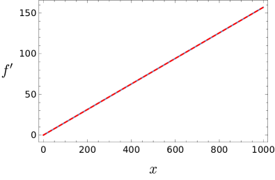
Figure 7: CEL solution: first derivative of the potential $f^{\prime}(x)$ for $h^{2}=10^{-4}$, $P=1/2$ and $\xi_{2}=\hat{\lambda}_{2}^{+}$ as in Eq. (16). The numerical solution of the full one-loop flow equation obtained from the pseudo-spectral method (solid blue line) lies exactly on top of the analytic solution in Eq. (70) for $C_{\mathrm{f}}=0$ (red dashed line).

VIII.1 Pseudo-spectral methods

Pesudo-spectral methods provide for a powerful tool to numerically solve functional RG equations, provided the desired solution can be spanned by a suitable set of basis functions. Here, we are interested in a numerical construction of global properties of the QFP function $f(x)$. We follow the method presented in Borchardt and Knorr (2015), as this approach has proven to be suited for this purpose, see Borchardt et al. (2016); Borchardt and Knorr (2016); Borchardt and Eichhorn (2016); Heilmann et al. (2015) for a variety of applications, and Fischer and Gies (2004) for earlier FRG implementations; a more general account of pseudo-spectral methods can be found in Boyd (2000); Robson and Prytz (1993); Ansorg et al. (2003); Macedo and Ansorg (2014).

In order to solve the differential equation given by Eq. (92) globally on $\mathbb{R}_{+}$, the strategy is to decompose the potential $f(x)$ into two series of Chebyshev polynomials. The first series is defined over some domain $[0,x_{\mathrm{M}}]$ and is spanned in terms of Chebyshev polynomials of the first kind $T_{i}(z)$. The second series is defined over the remaining infinite domain $[x_{\mathrm{M}},+\infty)$ and expressed in terms of rational Chebyshev polynomials $R_{i}(z)$. Moreover, to capture the correct asymptotic behavior of $f(x)$, the latter series is multiplied by the leading asymptotic term $x^{d/d_{x}}$, which is in fact the solution of the homogeneous scaling part of Eq. (92). Finally the ansatz reads

$$f(x)=\left\{\begin{aligned} &\sum_{i=0}^{N_{a}}\,a_{i}\,T_{i}\left(\frac{2x}{x_{\mathrm{M}}}-1\right),&\quad x\leq x_{\mathrm{M}},\\ &x^{\frac{d}{d_{x}}}\,\sum_{i=0}^{N_{b}}\,b_{i}\,R_{i}\bigl{(}x-x_{\mathrm{M}}),&\quad x\geq x_{\mathrm{M}}.\end{aligned}\right.$$ (107)

We thus convert the initial equation into an algebraic set of $N_{a}+N_{b}+2$ equations that can be solved applying the collocation method, for example by choosing the roots of $T_{N_{a}+1}$ and $R_{N_{b}+1}$. At the matching point $x_{\mathrm{M}}$, the continuity of $f(x)$ and $f^{\prime}(x)$ must be taken into account. The solutions presented in the following are obtained by choosing $x_{\mathrm{M}}=2$. We have further examined that the results do not change once $x_{\mathrm{M}}$ is varied.

In Fig. 7, we compare the first derivative $f^{\prime}(x)$ obtained from this pseudo-spectral method and the analytical solution derived from the $\phi^{4}$-dominance EFT approximation, see Eq. (70), for a fixed value of $h^{2}=10^{-4}$ and $\xi_{2}=\hat{\lambda}_{2}^{+}$. The two solutions lie perfectly on top of each other within the numerical error. Moreover, the coefficients $a_{i}$ and $b_{i}$ exhibit an exponential decay with increasing $N_{a}$ and $N_{b}$ – and thus indicate an exponentially small error of the numerical solution – until the algorithm hits machine precision.

The pseudo-spectral method thus allows us to provide clear numerical evidence for the global existence of the CEL solution within the full non-linear flow equation in the one-loop approximation. To our knowledge, this is the first time that results about global stability have been obtained for the scalar potential of this model.

We emphasize that the expansion around the origin in Chebyshev polynomials is an expansion over a set of basis functions that are in $C^{\infty}$. Unfortunately, they do not form a suitable basis for the new QFP solutions parametrized by $C_{\mathrm{f}}(\xi_{2})$ as in Eq. (85), because of the presence of the log-type singularity at the origin. Naively applying the same pseudo-spectral methods to this case does, in fact, not lead to numerically stable results.

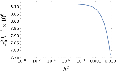
Figure 8: The ratio $x_{0}^{2}/h^{2}$ as a function of $h^{2}$ for $P=1/2$ and $\xi_{2}=10$. The solid line represents the numerical solution from the shooting from the minimum whereas the dashed line represents the analytic solution, which can be found in Eq. (84).

VIII.2 Shooting method

Let us therefore use the shooting method that allows to deal with the presence of the log-singularity to some extent. For this, we integrate Eq. (92) starting from the minimum $x_{0}$ towards both the origin and infinity. The boundary conditions that have to be fulfilled are

$$f^{\prime}(x_{0})=0,\quad f^{\prime\prime}(x_{0})=\xi_{2},$$ (108)

which are just the definitions of the minimum and the quartic coupling. The set of parameters is $x_{0}$, $\xi_{2}$, and $h^{2}$. For the present type of equations, it is well known that the integration outwards $x\to+\infty$ is spoiled by the presence of a movable singularity $x_{s+}$ Morris (1998, 1996, 1994b); Codello (2012); Codello and D’Odorico (2013); Vacca and Zambelli (2015). Here, the solutions from shooting develop a peak of maximum value of $x_{s+}$ only for a particular choice of initial parameters. In the latter 3-dimemsional space, we therefore have a surface that can be parametrized, for example, by $x_{0}(\xi_{2},h^{2})$. In the $\phi^{4}$-dominance EFT, we have seen that the leading contribution in $h^{2}$ to the nontrivial minimum $x_{0}$ is given by Eq. (84) for $P=1/2$. Fig. 8 shows how the full numerical solution converges to the analytical one in the limit $h^{2}\to 0$ for the fixed value of $\xi_{2}=10$. Repeating the numerical analysis for different values of $\xi_{2}>4$, we find a similar agreement with the analytic solution in all studied cases.

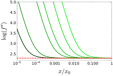
Figure 9: $\text{Log}\,(f^{\prime\prime})$ as a function of $x/x_{0}$ for $P=1/2$ and fixed value of $\xi_{2}=10$. Comparison between the numerical solutions from the shooting from the minimum (solid lines) and the analytic ones (dashed lines) for different values of the Yukawa coupling: $h^{2}\in\{10^{-8},10^{-7},10^{-6},3\cdot 10^{-5},10^{-4},6\cdot 10^{-4},3\cdot 10^{-3}\}$ from the darker (left) to the lighter (right) curve.

Additionally, we have also seen in the $\phi^{4}$-dominance EFT approximation that the family of solutions with a nontrivial minimum are singular at the origin from the second derivative on. Very close to the origin this fixed singularity in $f^{\prime\prime}(x)$ may spoil standard integration algorithms and the numerical integration stops at some $x_{s-}$ value. This kind of feature has been studied also in the non-abelian Higgs model Gies and Zambelli (2017). In principle, these singularities in higher derivatives could contradict asymptotic freedom if they persisted in the $h^{2}\to 0$ limit. To verify that this is not the case, we first analyze the behavior of $f^{\prime\prime}(x)$ close to the origin and compare it to the analytic one. From Eq. (70), we know that the term responsible for the fixed singularity is the scaling term $C_{\mathrm{f}}x^{d/d_{x}}=C_{\mathrm{f}}x^{4/(2+\eta_{x})}$. Indeed, taking the log of the second derivative gives

$$\log f^{\prime\prime}(x)\sim-\frac{2\eta_{x}}{2+\eta_{x}}\log x\quad\text{for $x\to 0$}.$$ (109)

In Fig. 9, we depict how the numerical solutions (green lines) deviate from this analytic one (dashed line) close to the origin and for different values of $h^{2}$ at fixed $\xi_{2}=10$. This plot shows that the region of discrepancy progressively shrinks as $h^{2}$ gets smaller and smaller: indeed for smaller values of $h^{2}$ the point where the numerical solution deviates from the analytic one moves towards smaller values. To measure this region, we have determined the onset of the singularity close to the origin as a function of $h^{2}$. Following the same idea as in Gies and Zambelli (2017), the criteria is to compute the position of $x_{s-}$ where $f^{\prime\prime}(x_{s-})$ assumes a sufficiently large value, let us say $\log f^{\prime\prime}(x_{s-})=4$. An estimate of $x_{s-}$ is shown in Fig. 10 where a fit of the data confirms that the singular region shrinks to zero for $h^{2}\to 0$. In fact we have found numerically a power law $x_{s-}\sim h^{2a}$ with $a\simeq 1.084$ for the present model.

We conclude that the existence of the new solutions is confirmed with the shooting method. We find satisfactory qualitative agreement with the solutions identified in the $\phi^{4}$-dominance effective field theory approximation, which are singular at the origin and show a nontrivial minimum.

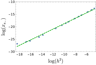
Figure 10: Measure of the singular region due to the presence of the fixed singularity in $x=0$ as a function of $h^{2}$. The with is estimated by the criteria $f^{\prime\prime}(x_{s-})=4$. For fixed $\xi_{2}=10$ we have found that the numerical points are well approximated by the power law (dashed line) $x_{s-}\sim h^{2a}$ where $a\simeq 1.084$.

IX Conclusions

Models that feature the existence of asymptotically free RG trajectories represent “perfect” quantum field theories in the sense that they could be valid and consistent models at any energy and distance scale. Identifying such RG trajectories hence provides information that can be crucial for our attempt at constructing fundamental models of particle physics. Based on the observation that part of the standard model including the Higgs-top sector exhibits a behavior reminiscent to an asymptotically free trajectory, we have taken a fresh look at asymptotic freedom in a gauged-Yukawa model from a perspective that supersedes conventional studies within standard perturbation theory.

Gauged-Yukawa models form the backbone not only of the standard model, but also of many models of new physics. Our study concentrates on the simplest model, a $\mathbbm{Z}_{2}$-Yukawa-QCD model, that features asymptotically free trajectories already in standard perturbation theory as first found in Ref. Cheng et al. (1974). Using effective-field-theory methods as well as various approximations based on the functional RG, we discover additional asymptotically free trajectories. One key ingredient for this discovery is a careful analysis of boundary conditions on the correlation functions of the theory, manifested by the asymptotic behavior of the Higgs potential in field space in our study. Whereas standard perturbation theory corresponds to an implicit choice of these boundary conditions, generalizing this choice explicitly yields a further two-parameter family of asymptotically free trajectories.

Our findings in this work generalize the strategy developed in Refs. Gies and Zambelli (2015, 2017) for gauged-Higgs models to systems including a fermionic matter sector. The new solutions also share the property that the quasi-fixed-point potentials, i.e., the solution to the fixed-point equation for a given small value of the gauge coupling, exhibit a logarithmic singularity at the origin in field space. Nevertheless, standard criteria (polynomial boundedness of perturbations, finiteness of the potential and its first derivative, global stability) are still satisfied. Moreover, since the quasi-fixed-point potential exhibits a nonzero minimum at any scale, correlation functions defined in terms of derivatives at this minimum remain well-defined to any order. Hence, we conclude that our solutions satisfy all standard criteria that are known to be crucial for selecting physical solutions in statistical-physics models Morris (1996); O’Dwyer and Osborn (2008); Bridle and Morris (2016).

The occurrence of a nontrivial minimum in the quasi-fixed-point solutions also indicates that standard arguments based on asymptotic symmetry Lee and Weisberger (1974) are sidestepped: conventional perturbation theory often focuses on the deep Euclidean region (DER), thereby implicitly assuming the irrelevance of nonzero minima or running masses for the RG analysis. In fact, all our new solutions demonstrate that the inclusion of a nonzero minimum is mandatory to reveal their existence. In this sense, the CEL solution found in standard perturbation theory is just a special case that features the additional property of asymptotic symmetry.

Our analysis is capable of extracting information about the global shape of the quasi-fixed-point potential. In fact, the requirement of global stability leads to constraints in the two-parameter family of solutions. The scaling exponent is confined to the values $P\leq 1/2$. This constraint is new in the present model in comparison with gauged-Higgs models Gies and Zambelli (2015, 2017), and may be indicative for the fact that further structures in the matter sector may lead to further constraints. The CEL solution is a special solution with $P=1/2$, such that our results provide direct evidence for the first time that the CEL solution indeed features a globally stable potential.

In our work, we so far concentrated on the flow of the effective potential $u(\rho)$ (or $f(x)$). This does, of course, not exhaust all possible structures that may be relevant for identifying asymptotically free trajectories. A natural further step would be a study of a full Yukawa coupling potential $h(\rho)$. This would generalize the single Yukawa coupling $h$ which corresponds to the coupling defined at the minimum $h(\rho=\kappa)$. In fact, the functional RG methods are readily available to also deal with this additional layer of complexity Zanusso et al. (2010); Vacca and Zanusso (2010); Pawlowski and Rennecke (2014); Braun et al. (2014); Vacca and Zambelli (2015); Jakovac et al. (2016b); Knorr (2016); Gies et al. (2017). As further boundary conditions have to be specified, it is an interesting open question as to whether the set of asymptotically free trajectories becomes more diverse or even more constrained.

In view of the standard model with its triviality problem arising from the U(1) hypercharge sector, it also remains to be seen if our construction principle can be applied to this U(1) sector. We believe that the construction of UV complete quantum field theories with a U(1) factor as part of the fundamental gauge-group structure should be a valuable ingredient in contemporary model building.

Appendix A More perturbatively renormalizable asymptotically free solutions

In this Appendix, we complete the review of perturbatively renormalizable AF solutions allowed at one loop for the $\mathbbm{Z}_{2}$-Yukawa-QCD model defined in Eq. (1). Our analysis is partly similar to that of Ref. Giudice et al. (2015), but generalizes it with the notion of QFPs. The flow in the $(g_{\mathrm{s}}^{2},h^{2})$ plane, provided by Eq. (2) and Eq. (3), is best understood by direct analytic integration of the RG equations, and adopting $g_{\mathrm{s}}^{2}$ as an (inverse) RG time. The solution of the flow reads

$$h^{2}(g_{\mathrm{s}}^{2})=\frac{g_{\mathrm{s}}^{2}}{c\,g_{\mathrm{s}}^{2(1-\gamma)}+1/\hat{h}_{*}^{2}},$$ (110)

where

$$\gamma=\frac{9}{11N_{\mathrm{c}}-2N_{\mathrm{f}}}\frac{N_{\mathrm{c}}^{2}-1}{N_{\mathrm{c}}}.$$ (111)

The QFP $\hat{h}_{*}^{2}$ is defined in Eq. (5) and $c$ is an integration constant. Notice that $\gamma$ as defined in Eq. (111) is positive as long as $g_{\mathrm{s}}^{2}$ is AF, according to Eq. (2). Also, the condition $\hat{h}_{*}^{2}>0$, which further restricts the viable field content as in Eq. (7), is equivalent to $\gamma>1$, as follows from Eq. (111). In fact, the standard-model case, $N_{\mathrm{c}}=3$ and $N_{\mathrm{f}}=6$, leads to $\gamma=8/7$. If one initializes the flow at some arbitrary RG scale $\Lambda$, with a gauge coupling $g_{\mathrm{s}\Lambda}^{2}$ and a Yukawa coupling $h_{\Lambda}^{2}$, then $c$ is given by

$$c\,g_{\mathrm{s}\Lambda}^{2(1-\gamma)}=\left(\frac{g_{\mathrm{s}}^{2}}{h^{2}}\right)_{\!\!\Lambda}-1/\hat{h}_{*}^{2}.$$ (112)

There is only one trajectory along which $h^{2}$ exhibits an asymptotic scaling proportional to $g_{\mathrm{s}}^{2}$, and it corresponds to $h^{2}_{\Lambda}=g^{2}_{\text{s}\Lambda}\,\hat{h}_{*}^{2}$ and $c=0$. If the initial condition is chosen in this way, the strong coupling drives the Yukawa coupling to zero in the UV. If instead the initial condition is different, then $c\neq 0$ in Eq. (110) and the fate of the system depends on the sign of $c$. For $c<0$, which corresponds to $\hat{h}_{\Lambda}^{2}>\hat{h}_{*}^{2}$ according to Eq. (112), either $h^{2}<0$ for all $g_{\mathrm{s}}^{2}<1$, or $h_{\Lambda}^{2}>0$ and the Yukawa coupling hits a Landau pole in the UV, i.e., it diverges at a finite RG time. For $c>0$, namely $\hat{h}_{\Lambda}^{2}<\hat{h}_{*}^{2}$, there is no Landau pole and the trajectories are also AF, but with an asymptotic scaling that differs from the one defined by Eq. (4) and Eq. (5). In fact, in this case

$$h^{2}(g_{\mathrm{s}}^{2})\mathrel{\underset{g_{\mathrm{s}}\to 0}{\scalebox{2.0}[1.0]{$\sim$}}}\frac{1}{c}\,g_{\mathrm{s}}^{2\gamma},$$ (113)

for any $c\neq 0$, thanks to the assumption that Eq. (7) holds, such that $\gamma>1$. Also this scaling solution should be amenable to an interpretation as a QFP for the flow of a suitable ratio. Indeed, we could define

$$\hat{h}^{\prime\,2}=\frac{h^{2}}{g_{\mathrm{s}}^{2\gamma}}.$$ (114)

For this ratio we would find the following $\beta$ function

$$\partial_{t}\hat{h}^{\prime\,2}=\frac{9g_{\mathrm{s}}^{2\gamma}}{16\pi^{2}}\hat{h}^{\prime\,4}.$$ (115)

Here the second term in Eq. (3) has been canceled by the contribution $-\gamma\eta_{A}\hat{h}^{\prime\,2}$ coming from the rescaling, due to the value of $\gamma$ given in Eq. (111). While Eq. (115) does not vanish for any finite value of the strong coupling constant $g_{\mathrm{s}}^{2}\neq 0$, the fact that the would-be-leading contribution proportional to $g_{\mathrm{s}}^{2}$ vanishes for any $\hat{h}^{\prime\,2}$ signals the presence of a QFP with arbitrary value of $\hat{h}^{\prime\,2}$. This is only approximately realized at finite $g_{\mathrm{s}}^{2}\neq 0$ and becomes exact in the $g_{\mathrm{s}}^{2}\to 0$ limit.

Let us now address the stability properties of the AF trajectories plotted in Fig. 1. From the previous discussion it is clear that an infinitesimal perturbation of a trajectory characterized by $c\neq 0$, along a direction which changes the value of the Yukawa coupling, i.e., $c$ itself, results in a new trajectory which is still a scaling solution. Thus, one moves from a given $\hat{h}^{\prime\,2}$ to another $\hat{h}^{\prime\,2}+\delta\hat{h}^{\prime\,2}$, and the distance between the two trajectories stays constant in RG time in the UV limit if measured in terms of the rescaled coupling $\hat{h}^{\prime\,2}$. Hence, we can call this a marginal perturbation. These QFP solutions are neither stable nor unstable. Yet, as it is clear from the left panel of Fig. 1, quantification of the distance between trajectories in terms of the unrescaled $h^{2}$ would lead to a different conclusion, since such a distance would decrease as $g^{2}\to 0$. The unique trajectory with $c=0$ has a rather different behavior, as already discussed in Sec. II.

The AF solutions of Eq. (113) in the Yukawa sector, translate into corresponding AF trajectories in the Higgs sector. As we did for the CEL solution, we inspect the running of the finite ratio $\hat{\lambda}_{2}$ defined in Eq. (11), and $P$ still to be determined. We restrict $h^{2}$ such that the ratio in Eq. (114) attains an arbitrary finite value in the UV. In this case, the reduced anomalous dimension enters the $\beta$ function of $\hat{\lambda}_{2}$ of Eq. (15),

$$\eta_{h^{2}}^{\prime}=\left[-\frac{\partial_{t}h^{2}}{h^{2}}\right]_{h^{2}=g_{\mathrm{s}}^{2\gamma}\hat{h}^{\prime\,2}}\mathrel{\underset{g_{\mathrm{s}}\to 0}{\scalebox{2.0}[1.0]{$\sim$}}}\frac{3}{8\pi^{2}}\frac{N_{\mathrm{c}}^{2}-1}{N_{\mathrm{c}}}g_{\mathrm{s}}^{2},$$ (116)

where we have neglected a second contribution which is proportional to $g_{\mathrm{s}}^{2\gamma}$, since $\gamma>1$. Inserting this into the flow equation for $\hat{\lambda}_{2}$ and replacing $g_{\mathrm{s}}^{2}=(c\,h^{2})^{1/\gamma}$, where $c^{-1}>0$ is the QFP value of $\hat{h}^{\prime\,2}$, one gets four terms. Each of these terms scales with a different power of $h^{2}$. In order to have a QFP solution with a positive $\hat{\lambda}_{2}$, it is necessary that the contributions from the fermions be the leading ones, which requires

$$P=1-\frac{1}{2\gamma},$$ (117)

and results in

$$\hat{\lambda}_{2}=\frac{N_{\mathrm{c}}^{2}}{3(N_{\mathrm{c}}^{2}-1)}\frac{1}{\big{(}1-\frac{1}{2\gamma}\big{)}c^{1/\gamma}}.$$ (118)

Notice that these QFPs do not correspond to any trajectory plotted in Fig. 2, because they lie on a different hypersurface in the $\{g_{\mathrm{s}}^{2},h^{2},\lambda\}$ space, with a scaling defined by Eq. (114) rather then Eq. (4). Still, one can produce similar plots on the hypersurface corresponding to Eq. (114), and they would look very similar to those shown in Fig. 2. In fact, due to the positive sign of $\eta_{h^{2}}$, also the QFP in Eq. (118) is UV repulsive, meaning that for a chosen initialization value of $h^{2}$, i.e., one $c$, there is only one AF trajectory for $\lambda_{2}$ approaching the Gaußian fixed point from positive values, and it corresponds to Eq. (118). Larger values of $\hat{\lambda}_{2}$ would result in a Landau pole, while smaller values would lead to negative $\lambda_{2}$ at high energy.

Appendix B Large field behavior of the asymptotically free potentials

B.1 EFT resummation of the effective potential in the DER

For a study of the stability of the potential $u(\rho)$ (see Eq. (40)) in the UV, it is necessary to address the combined limit $\rho\to\infty$ and $h^{2}\to 0$. However, a meaningful and consistent result requires to take these limites in an appropriate order while remaining in the outer or inner asymptotic region, defined respectively as the region where the variable $z=h^{2}\rho$ appearing in the bosonic and fermionic threshold functions is $z\gg 1$ or $z\ll 1$ as introduced in Sec. VI.

Let us start with the outer region. If $h^{2}$ is small and finite we can address the asymptotic behavior by expanding the potential of Eq. (40) for $z\to\infty$. This gives the following result

$$u(\rho) =\frac{\hat{\lambda}_{2}z^{2}}{2h^{2}}+\Gamma\left(\frac{4+4\eta_{z}}{2+\eta_{z}}\right)\frac{1}{32\pi^{2}(2+3\eta_{z})}\times$$

$$\quad\times\Bigg{\{}\frac{\Gamma\left(\frac{2\eta_{z}}{2+\eta_{z}}\right)}{\Gamma\left(\frac{2+3\eta_{z}}{2+\eta_{z}}\right)^{2}}3z^{2}(3\hat{\lambda}_{2}^{2}-4)$$

$$\quad+\Gamma\left(\frac{-2\eta_{z}}{2+\eta_{z}}\right)z^{\frac{4}{2+\eta_{z}}}\bigl{[}(3\hat{\lambda}_{2})^{\frac{4}{2+\eta_{z}}}-12\bigr{]}\Bigg{\}}$$

$$\quad+\mathcal{O}(z)\Big{|}_{z=h^{2}\rho}$$

$$\equiv\left[\frac{\hat{\lambda}_{2}}{2h^{2}}+c_{1}(h^{2})\right]z^{2}+c_{2}(h^{2})\,z^{\frac{4}{2+\eta_{z}}}+\mathcal{O}(z)\Big{|}_{z=h^{2}\rho}$$ (119)

where $\eta_{z}$ is the anomalous dimension of $z$ as given in Eq. (37). Now we can safely perform the limit $h^{2}\to 0$ in the outer asymptotic region where $z\gg 1$. We find that the leading order behavior is given only by the first term, as in Eq. (42). Indeed the noninteger power scaling $z^{4/(2+\eta_{z})}$ behaves as $z^{2}$ for $h^{2}\to 0$ and the two coefficients $c_{1}$ and $c_{2}$ have simple poles in $h^{2}$ that cancel each other in the limit $h^{2}\to 0$.

Let us further consider the inner interval. Expanding the potential of Eq. (40) for small $h^{2}$, we obtain the following expression:

$$u(\rho) =\frac{\hat{\lambda}_{2}}{h^{2}}\frac{z^{2}}{h^{2}}+\frac{3z^{2}}{32\pi^{2}(2+3\eta_{z})}\Bigl{[}3\hat{\lambda}_{2}^{2}\log(1+3\hat{\lambda}_{2}z)$$

$$\quad-4\log(1+z)\Bigr{]}+b_{2}(z)\frac{\eta_{z}z^{2}}{2+3\eta_{z}}+\mathcal{O}(h^{4}z^{2}).$$ (120)

The function $b_{2}(z)$ goes to zero with $z$, as is also true for the second term. This expansion is valid only for those values of $\rho$ such that $h^{2}\rho\ll 1$. Therefore for addressing the limit $\rho\to\infty$, it is necessary to take the limit $h^{2}\to 0$ while keeping $z\ll 1$, in such a way that the expansion in Eq. (120) still holds. Doing so, we find that the leading term for the potential is again the one in Eq. (42) also in the inner asymptotic region. The same conclusion can be deduced by expanding the potential for small $z$ and keeping $h^{2}$ fixed. Indeed the function $u(\rho)$ is analytic in $z$ and its expansion reads

$$u(\rho)=\frac{\hat{\lambda}_{2}}{2}\frac{z^{2}}{h^{2}}+\frac{27\hat{\lambda}_{2}^{3}-12}{32\pi^{2}(2+3\eta_{z})}z^{3}+\mathcal{O}(z^{4}),$$ (121)

where again the $h^{2}\to 0$ limit with fixed $z\ll 1$ gives us the result in Eq. (42).

Let us emphasize once more that a consistent answer about the full stability of the potential $u(\rho)$ requires to take the two limits $\rho\to\infty$ and $h^{2}\to 0$ in such a way that the variable $z=h^{2}\rho$ entering the bosonic and fermionic loops controllably satisfies $z\gg 1$ (outer region) or $z\ll 1$ (inner region). In these two asymptotic regions, the potential has the same positive asymptotic coefficient in front of the leading quadratic term. Therefore, we conclude that it is stable for arbitrarily small values of the Yukawa coupling.

B.2 $f(x)$ in the $\phi^{4}$-dominance approximation

In Sec. VI, the same reasoning for taking the asymptotic limits as in the preceding section applies to the two loop-variables $z_{\mathrm{B}}$ and $z_{\mathrm{F}}$, defined in Eq. (71). Let us start by inspecting the potential $f(x)$ in the $\phi^{4}$-dominance approximation first in the outer region. For finite values of $h^{2}$, we can assume that the loop contributions are negligible for large field amplitudes and therefore expand the scalar and fermionic loops in powers of $x^{-1}$. Setting the left-hand side of Eq. (68) to zero, the QFP potential can then be expressed in terms of an infinite series

$$f_{\text{as}}(x) =-\frac{1}{32\pi^{2}}\sum_{n=1}^{\infty}(-)^{n}\frac{1-12\,(3h^{2(2P-1)}\xi_{2})^{n}}{\left(3\xi_{2}h^{2P}x\right)^{n}(4+2n+n\eta_{x})}$$

$$\quad+C_{\text{as}}\,x^{\frac{4}{2+\eta_{x}}},$$ (122)

which can be resummed analytically

$$f_{\text{as}}(x)=C_{\text{as}}x^{\frac{4}{2+\eta_{x}}}+\frac{1}{32\pi^{2}(6+\eta_{x})}\times$$

$$\times\Biggl{[}\frac{1}{3\xi_{2}h^{2P}x}\,_{2}F_{1}\left(1,\frac{6+\eta_{x}}{2+\eta_{x}},\frac{8+2\eta_{x}}{2+\eta_{x}},-\frac{1}{3\xi_{2}h^{2P}x}\right)$$

$$-\frac{12}{h^{2(1-P)}x}\,_{2}F_{1}\left(1,\frac{6+\eta_{x}}{2+\eta_{x}},\frac{8+2\eta_{x}}{2+\eta_{x}},-\frac{1}{h^{2(1-P)}x}\right)\Biggr{]}.$$ (123)

Using the following linear transformation among the hypergeometric functions

$$\frac{\sin\left(\pi(b-a)\right)}{\pi\Gamma(c)}\,_{2}F_{1}(a,b,c,z)=$$

$$=\frac{1}{(-z)^{a}}\frac{{}_{2}F_{1}\left(a,a-c+1,a-b+1,z^{-1}\right)}{\Gamma(b)\Gamma(c-a)\Gamma(a-b+1)}$$

$$-\frac{1}{(-z)^{b}}\frac{{}_{2}F_{1}\left(b,b-c+1,b-a+1,z^{-1}\right)}{\Gamma(a)\Gamma(c-b)\Gamma(b-a+1)},$$ (124)

it is possible to rewrite the solution $f(x)$ into $f_{\text{as}}(x)$. Indeed, this becomes clear from the relation between the two integration constants $C_{\mathrm{f}}$ and $C_{\text{as}}$ which is

$$C_{\text{as}} =C_{\mathrm{f}}+\frac{\pi}{2+\eta_{x}}\left[\sin\left(\frac{4\pi}{2+\eta_{x}}\right)\right]^{-1}h^{\frac{8(1-P)}{2+\eta_{x}}}\times$$

$$\times\frac{1}{32\pi^{2}}\left[\left(3\xi_{2}h^{2(2P-1)}\right)^{\frac{4}{2+\eta_{x}}}-12\right].$$ (125)

This mapping from $f_{\text{as}}(x)$ to $f(x)$ tells us that the asymptotic behavior of the QFP solution is determined in the outer asymptotic region, where $z_{\mathrm{B}/\mathrm{F}}\gg 1$, only by the scaling terms in $\partial_{t}f(x)=0$. In fact, this property can be inferred also by expanding the solution $f(x)$, instead of its beta function, for large $z_{\mathrm{B}/\mathrm{F}}$

$$f(x) =C_{\mathrm{f},\infty}\,x^{\frac{4}{2+\eta_{x}}}+\frac{\Gamma\left(-\frac{6+\eta_{x}}{2+\eta_{x}}\right)\Gamma\left(\frac{-2+\eta_{x}}{2+\eta_{x}}\right)}{128\pi^{2}\,\Gamma\left(-\frac{4}{2+\eta_{x}}\right)^{2}}\times$$

$$\quad\times\Biggl{[}-\frac{12}{z_{\mathrm{F}}}+\frac{1}{z_{\mathrm{B}}}+\mathcal{O}\left(z_{\mathrm{B}}^{-2}\right)+\mathcal{O}\left(z_{\mathrm{F}}^{-2}\right)\Biggr{]}.$$ (126)

The coefficient in front of the scaling term is a function of $C_{\mathrm{f}}$, $\xi_{2}$, $h^{2}$, and $P$

$$C_{\mathrm{f},\infty} =C_{\mathrm{f}}+\frac{1}{128\pi^{2}}\Gamma\left(\frac{-2+\eta_{x}}{2+\eta_{x}}\right)\Gamma\left(\frac{6+\eta_{x}}{2+\eta_{x}}\right)\times$$

$$\quad\times\left[\left(3\xi_{2}h^{2P}\right)^{\frac{4}{2+\eta_{x}}}-12\,h^{\frac{8(1-P)}{2+\eta_{x}}}\right].$$ (127)

It is not surprising that this scaling factor is exactly the asymptotic coefficient $C_{\text{as}}$. By using one of the defining properties of the Gamma function, $\Gamma(1+z)=z\Gamma(z)$ as well as the following identity

$$\Gamma(z)\Gamma(1-z)=\frac{\pi}{\sin(\pi z)},$$ (128)

we recover precisely the expression in Eq. (125), therefore

$$C_{\mathrm{f},\infty}=C_{\text{as}}.$$ (129)

As we are interested in the asymptotic behavior in the UV, it is convenient to expand Eq. (127) for small $h^{2}$ and keep only the leading terms,

$$C_{\mathrm{f},\infty}\mathrel{\underset{h^{2}\to 0}{\scalebox{2.0}[1.0]{$\sim$}}}C_{\mathrm{f}}-\frac{9\xi_{2}^{2}h^{2(2P-1)}-12\,h^{2(1-2P)}}{64\pi^{2}\hat{\eta}_{x}}.$$ (130)

Moreover, all the subleading terms in Eq. (126) of order $\mathcal{O}(z_{\mathrm{B}}^{-1})$ and $\mathcal{O}(z_{\mathrm{F}}^{-1})$ are regular in the $h^{2}\to 0$ limit. We can thus conclude that the asymptotic property of the QFP potential is correctly described by Eq. (130) both in the outer region, i.e., for large field amplitudes, and in the UV limit.

Let us address now the situation in the inner region, where we can expand the potential $f(x)$ either for $z_{\mathrm{B}/\mathrm{F}}\ll 1$ or for $x\ll 1$ while keeping $h^{2}$ finite. In both cases the result is the same, and reads

$$f(x) =-\frac{11}{128\pi^{2}}+C_{\mathrm{f}}x^{\frac{4}{2+\eta_{x}}}-\frac{z_{\mathrm{B}}-12z_{\mathrm{F}}}{32\pi^{2}(2-\eta_{x})}$$

$$\quad-\frac{z_{\mathrm{B}}^{2}-12z_{\mathrm{F}}^{2}}{64\pi^{2}h^{2}\hat{\eta}_{x}}+\mathcal{O}(z_{\mathrm{B}}^{3})+\mathcal{O}(z_{\mathrm{F}}^{3}).$$ (131)

In the UV limit, the inner region increases and thus allows to address the asymptotic behavior of the potential. Indeed this combined limit can be taken as long as $z_{\mathrm{B}/\mathrm{F}}\ll 1$ holds. From Eq. (131), we can deduce that

$$f(x)\mathrel{\underset{x\to\infty}{\scalebox{2.0}[1.0]{$\sim$}}}\left[C_{\mathrm{f}}-\frac{9\xi_{2}^{2}h^{2(2P-1)}-12h^{2(1-2P)}}{64\pi^{2}\hat{\eta}_{x}}\right]x^{2},$$ (132)

where the coefficient in front of the quadratic term coincides with Eq. (130). The same information is obtained by expanding the hypergeometric functions in Eq. (70) for small Yukawa coupling,

$$f(x)=C_{\mathrm{f}}x^{\frac{4}{2+\eta_{x}}}-\frac{z_{\mathrm{B}}^{2}-12\,z_{\mathrm{F}}^{2}}{64\pi^{2}h^{2}\hat{\eta}_{x}}+\mathcal{O}(h^{0}).$$ (133)

This is in agreement with Eq. (132) for the asymptotic behavior within the inner region.

We finally conclude that it is possible to simultaneously take the $x\to\infty$ limit and the $h^{2}\to 0$ limit in both the inner and outer asymptotic regions. This combined limit gives the same result in both regions, and can be summarized as

$$f(x)\mathrel{\underset{\begin{subarray}{c}x\to\infty\\ h^{2}\to 0\end{subarray}}{\scalebox{3.0}[1.0]{$\sim$}}}h^{\pm 2(2P-1)}\,\,\hat{C}_{\mathrm{f},\infty}\,x^{2},$$ (134)

where the $\pm$ sign is for $P\lessgtr 1/2$. The expression for $\hat{C}_{\mathrm{f},\infty}$ can be found in the main text in Eq. (74).

B.3 Comparison between $u(\rho)$ and $f(x)$

The potential $u(\rho)$ in Eq. (40), obtained within the DER, and the effective potential $f(x)$ in Eq. (70), derived in the $\phi^{4}$-dominance approximation, can be related to each other by exploiting a general identity among the Gauß  hypergeometric functions

$$\frac{zb}{c}\,_{2}F_{1}(a+1,b+1,c+1,z)$$

$$=\,_{2}F_{1}(a+1,b,c,z)-\,_{2}F_{1}(a,b,c,z).$$ (135)

By setting $a=0$ in the latter expression, we get the following relationship

$${}_{2}F_{1}(1,b,c,z)=1+\frac{zb}{c}\,_{2}F_{1}(1,b+1,c+1,z).$$ (136)

Iterating this twice, we can rewrite the solution $f(x)$ as

$$f(x) =\frac{1}{32\pi^{2}}\Biggl{[}-\frac{11}{4}+\frac{4-\xi_{2}}{2-\eta_{x}}3hx+\frac{4-\xi_{2}^{2}}{2\eta_{x}}3h^{2}x^{2}$$

$$\quad+\frac{(3\xi_{2}hx)^{3}}{2+3\eta_{x}}\,_{2}F_{1}\left(1,\frac{2+3\eta_{x}}{2+\eta_{x}},\frac{4+4\eta_{x}}{2+\eta_{x}},-3\xi_{2}hx\right)$$

$$\quad-\frac{12(hx)^{3}}{2+3\eta_{x}}\,_{2}F_{1}\left(1,\frac{2+3\eta_{x}}{2+\eta_{x}},\frac{4+4\eta_{x}}{2+\eta_{x}},-hx\right)\Biggr{]}$$

$$\quad+C_{\mathrm{f}}\,x^{\frac{4}{2+\eta_{x}}}.$$ (137)

Let us consider the CEL potential corresponding to $P=1/2$, $C_{\mathrm{f}}=0$, and $\xi_{2}=\hat{\lambda}_{2}^{+}$. Working in the limit $h^{2}\to 0$ where we can take $\eta_{x}\to\eta_{z}$, cf. Eq. (69) and Eq. (37), Eq. (137) becomes

$$\lim_{\eta_{x}\to\eta_{z}}f(x)=u(\rho)\Big{|}_{x=h\rho}-\frac{11}{128\pi^{2}}+\frac{3hx(4-\xi_{2})}{32\pi^{2}(2-\eta_{z})}.$$ (138)

We conclude that the solution $f(x)$ becomes the solution $u(\rho)$ in the UV limit – apart from a linear term in the field variable that is, in fact, discarded by the definition of the deep euclidean approximation.

Appendix C The unphysical $P>1$ case

C.1 Effective-field-theory analysis

In Sec. V, we have encountered an example in the RG equations for $\hat{\lambda}_{2}$ and $\hat{\kappa}$ (cf. Eq. (56) and Eq. (57)) that for $P>1/2$ there are only few terms which may contribute to the leading part in the $h^{2}\to 0$ limit. This is a consequence of the remaining legitimate configuration for the scaling powers $P$, $Q$, and $P_{3}$. The situation is very similar also for $P>1$, where there are only two consistent solutions,

$$\hat{\kappa} =\mp\left(\frac{3}{8\pi^{2}\hat{\lambda}_{3}}\right)^{\frac{1}{4}},\quad\quad\quad Q =\frac{2P+1}{3},$$ (139)

$$\hat{\lambda}_{2} =\pm\frac{1}{2}\left(\frac{3\hat{\lambda}_{3}^{3}}{8\pi^{2}}\right)^{\frac{1}{4}},\quad\quad\quad P_{3} =\frac{8P+1}{3},$$ (140)

and

$$\hat{\lambda}_{2} =\frac{-2\pm\sqrt{2P-1}}{2(5-2P)\hat{\kappa}},\quad\quad\quad Q =2P,$$ (141)

$$\hat{\lambda}_{3}^{2} =\frac{8\pi^{2}(1+2\hat{\kappa}\hat{\lambda}_{2})^{4}}{(2P-1)\hat{\kappa}^{3}},\quad\quad\quad P_{3} =3P,$$ (142)

where $\hat{\lambda}_{3}$ is a free parameter. Moreover we notice that the scaling powers $Q$ and $P_{3}$ in Eq. (139) and Eq. (140) are the same as in the model discussed in Refs. Gies and Zambelli (2015, 2017). These analytical solutions are however unphysical due to the fact that positive $\hat{\kappa}$ correspond to negative $\hat{\lambda}_{2}$ and vice versa.

C.2 Weak-$h^{2}$ expansion

For $P>1$ the argument of the fermionic loop $\omega_{1f}$, defined in Eq. (93), diverges in the limit $h^{2}\to 0$ at fixed $x$. Therefore, in order to capture the correct UV behavior, one has to Taylor expand the threshold function $l_{0}^{(\mathrm{F})}(\omega_{1f})$ in powers of $\omega_{1f}^{-1}$. Let us start the investigation for $1<P<2$. In this case the leading $h^{2}$-dependent contribution to $\beta_{f}$ is

$$\delta\beta_{f} =-\frac{N_{\mathrm{c}}d_{\gamma}}{32\pi^{2}x}h^{2(P-1)} \text{for $1<P<2$},$$ (143)

and the integration of the QFP condition $\beta_{f}=0$ gives us the potential

$$f(x)=c\,x^{2}-\frac{N_{\mathrm{c}}d_{\gamma}}{192\pi^{2}x}h^{2(P-1)},$$ (144)

where $c$ is the integration constant of the first order ODE. The defining equation $f^{\prime}(x_{0})=0$ for the minimum fixes an expression for this integration constant $c(h^{2},x_{0})$, while the consistency condition $f^{\prime\prime}(x_{0})=\xi_{2}$ provides how $x_{0}$ is related to the parameters $\xi_{2}$ and $h^{2}$. Indeed

$$x_{0}^{3}=-\frac{N_{\mathrm{c}}d_{\gamma}}{64\pi^{2}\xi_{2}}h^{2(P-1)}.$$ (145)

By setting $N_{\mathrm{c}}=3$ and $d_{\gamma}=4$, the latter equation becomes

$$x_{0}^{3}=-\frac{3}{16\pi^{2}\xi_{2}}h^{2(P-1)},$$ (146)

showing an agreement with the EFT analysis including thresholds. Indeed, by taking Eqs. (139),(140) and recalling that $x_{0}=h^{2P}\kappa=h^{2(P-1)/3}\hat{\kappa}$, one gets exactly Eq. (146). Thus, there are no solutions with a nontrivial minimum for $\xi_{2}>0$.

It is worth to point out that the potential and all its derivatives are singular at the origin due to the Taylor expansion of $l_{0}^{(\mathrm{F})}(\omega_{1f})$ for small $\omega_{1f}^{-1}$, producing a term in $\delta\beta_{f}$ proportional to $x^{-1}$. This expansion is valid only for $x\gg h^{2(P-1)}$, a condition which is not fulfilled in the $x\to 0$ limit at fixed $h^{2}$. Yet, the fermionic loop is finite at the origin and this suggests to retain its whole $x$-dependence.

Accounting for the full fermionic loop still allows for an analytic solution of the QFP, which leads, for the piecewise linear cutoff regulator, to a Coleman-Weinberg-like potential

$$f(x) =c\,x^{2}+\frac{N_{\mathrm{c}}d_{\gamma}}{64\pi^{2}}\Biggl{[}\frac{x}{h^{2(P-1)}}$$

$$\quad+\frac{x^{2}}{h^{4(P-1)}}\log\Bigl{(}\frac{x}{x+h^{2(P-1)}}\Bigr{)}\Biggr{]}.$$ (147)

The corresponding quadratic rescaled scalar coupling, as a function of $h^{2}$ and $x_{0}$, reads

$$\xi_{2}=-\frac{N_{\mathrm{c}}d_{\gamma}}{64\pi^{2}}\frac{h^{2(P-1)}}{x_{0}\left(x_{0}+h^{2(P-1)}\right)^{2}},$$ (148)

which yields Eq. (146) in the $h^{2}\to 0$ limit for $N_{\mathrm{c}}=3$ and $d_{\gamma}=4$.

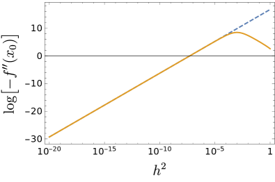
Figure 11: The rescaled quadratic coupling $\xi_{2}$ as a function of $h^{2}$ for $P=2$ and fixed value for the nontrivial minimum $x_{0}=10^{-3}$. Dashed line: EFT approximation including thresholds, see Eqs. (139),(140). Solid line: weak-$h^{2}$ expansion, see Eq. (153).

The situation is slightly different for $P\geq 2$ due to the contribution coming from the anomalous dimensions $\eta_{x}$ in the scaling part of $\beta_{f}$. Let us first expand the threshold function $l_{0}^{(\mathrm{F})}(\omega_{1f})$ in powers of $\omega_{1f}^{-1}$ such that the leading correction to the beta function is

$$\delta\beta_{f} =\hat{\eta}_{x}h^{2}xf^{\prime}-\frac{N_{\mathrm{c}}d_{\gamma}}{32\pi^{2}x}h^{2(P-1)}, \text{for $P\geq 2$}.$$ (149)

Due to the presence of a singular term at the origin, we expect that this pole survives also in the corresponding QFP solution which is in fact

$$f(x)=c\,x^{\frac{4}{2+\eta_{x}}}-\frac{N_{\mathrm{c}}d_{\gamma}}{(6+\eta_{x})}\frac{h^{2(P-1)}}{32\pi^{2}x}.$$ (150)

Additionally there is also a log-type singularity in the second derivative. Indeed by Taylor expanding the scaling term for small $h^{2}$, we get a term proportional to $x^{2}\log x$. This potential has a nontrivial minimum $x_{0}$ whose analytical expression in terms of $h^{2}$ and $\xi_{2}$ is

$$x_{0}^{3}=-\frac{N_{\mathrm{c}}d_{\gamma}}{32\pi^{2}\xi_{2}(2+\eta_{x})}h^{2(P-1)}.$$ (151)

If we instead consider the full fermionic loop, the general QFP solution reads

$$f(x) =-\frac{N_{\mathrm{c}}d_{\gamma}}{128\pi^{2}}\,_{2}F_{1}\left(1,-\frac{4}{2+\eta_{x}},\frac{-2+\eta_{x}}{2+\eta_{x}},-\frac{x}{h^{2(P-1)}}\right)$$

$$\quad+c\,x^{\frac{4}{2+\eta_{x}}}$$ (152)

where the Gauß hypergeometric function comes from the integration of the fermionic threshold function and it is analytic around the origin. The corresponding quadratic rescaled scalar coupling reads

$$\xi_{2}=-\frac{N_{\mathrm{c}}d_{\gamma}}{32\pi^{2}(2+\eta_{x})}\frac{h^{2(P-1)}}{x_{0}\left(x_{0}+h^{2(P-1)}\right)^{2}},$$ (153)

which is a generalization of Eq. (148) due to the anomalous dimension.

For all of these cases computed within the piecewise linear regulator, we can thus conclude that the weak-$h^{2}$ expansion for $P>1$ agrees with the EFT approximation including thresholds analyzed in Sec. C.1. In fact Eqs. (146), (148), (151), and (153) are all in agreement with Eqs. (139) and (140) in the $h^{2}\to 0$ limit and by fixing $N_{\mathrm{c}}=3$ and $d_{\gamma}=4$. In Fig. 11 we show indeed the rescaled quartic coupling $\xi_{2}$, i.e., the curvature of the potential at the nontrivial minimum $x_{0}$, as a function of the Yukawa coupling for fixed value of $x_{0}=10^{-3}$. The dashed line represents the EFT analysis, see Eqs. (139) and (140), whereas the solid line represents the weak-$h^{2}$ approximation in the case where the anomalous dimension $\eta_{x}$ and the full fermionic loop are taken into account, see Eq. (153).

So we summarize this section by emphasizing once more that for $P>1$ it is not possible to have a solution with a nontrivial minimum and at the same time a positive $\xi_{2}$.

References

- Gross and Wilczek (1973a) D. J. Gross and F. Wilczek, Phys. Rev. Lett. 30, 1343 (1973a).
- Politzer (1973) H. D. Politzer, Phys. Rev. Lett. 30, 1346 (1973).
- Gross and Wilczek (1973b) D. J. Gross and F. Wilczek, Phys. Rev. D8, 3633 (1973b).
- Cheng et al. (1974) T. P. Cheng, E. Eichten, and L.-F. Li, Phys. Rev. D9, 2259 (1974).
- Gross and Wilczek (1974) D. J. Gross and F. Wilczek, Phys. Rev. D9, 980 (1974).
- Politzer (1974) H. D. Politzer, Phys. Rept. 14, 129 (1974).
- Chang (1974) N.-P. Chang, Phys. Rev. D10, 2706 (1974).
- Chang and Perez-Mercader (1978) N.-P. Chang and J. Perez-Mercader, Phys. Rev. D18, 4721 (1978), [Erratum: Phys. Rev.D19,2515(1979)].
- Fradkin and Kalashnikov (1975) E. S. Fradkin and O. K. Kalashnikov, J. Phys. A8, 1814 (1975).
- Salam and Strathdee (1978) A. Salam and J. A. Strathdee, Phys. Rev. D18, 4713 (1978).
- Bais and Weldon (1978) F. A. Bais and H. A. Weldon, Phys. Rev. D18, 1199 (1978).
- Salam and Elias (1980) A. Salam and V. Elias, Phys. Rev. D22, 1469 (1980).
- Callaway (1988) D. J. E. Callaway, Phys. Rept. 167, 241 (1988).
- Giudice et al. (2015) G. F. Giudice, G. Isidori, A. Salvio, and A. Strumia, JHEP 02, 137 (2015), arXiv:1412.2769 [hep-ph] .
- Holdom et al. (2015) B. Holdom, J. Ren, and C. Zhang, JHEP 03, 028 (2015), arXiv:1412.5540 [hep-ph] .
- Hansen et al. (2017) F. F. Hansen, T. Janowski, K. Langaeble, R. B. Mann, F. Sannino, T. G. Steele, and Z.-W. Wang, (2017), arXiv:1706.06402 [hep-ph] .
- Hetzel and Stech (2015) J. Hetzel and B. Stech, Phys. Rev. D91, 055026 (2015), arXiv:1502.00919 [hep-ph] .
- Pelaggi et al. (2015) G. M. Pelaggi, A. Strumia, and S. Vignali, JHEP 08, 130 (2015), arXiv:1507.06848 [hep-ph] .
- Pica et al. (2016) C. Pica, T. A. Ryttov, and F. Sannino, (2016), arXiv:1605.04712 [hep-th] .
- Molgaard and Sannino (2016) E. Molgaard and F. Sannino, (2016), arXiv:1610.03130 [hep-ph] .
- Heikinheimo et al. (2017) M. Heikinheimo, K. Kannike, F. Lyonnet, M. Raidal, K. Tuominen, and H. Veermäe, JHEP 10, 014 (2017), arXiv:1707.08980 [hep-ph] .
- Buttazzo et al. (2013) D. Buttazzo, G. Degrassi, P. P. Giardino, G. F. Giudice, F. Sala, A. Salvio, and A. Strumia, JHEP 12, 089 (2013), arXiv:1307.3536 [hep-ph] .
- Bednyakov et al. (2015) A. V. Bednyakov, B. A. Kniehl, A. F. Pikelner, and O. L. Veretin, Phys. Rev. Lett. 115, 201802 (2015), arXiv:1507.08833 [hep-ph] .
- Di Luzio et al. (2015) L. Di Luzio, G. Isidori, and G. Ridolfi, (2015), arXiv:1509.05028 [hep-ph] .
- Andreassen et al. (2017) A. Andreassen, W. Frost, and M. D. Schwartz, (2017), arXiv:1707.08124 [hep-ph] .
- Alekhin et al. (2012) S. Alekhin, A. Djouadi, and S. Moch, Phys. Lett. B716, 214 (2012), arXiv:1207.0980 [hep-ph] .
- Bezrukov and Shaposhnikov (2015) F. Bezrukov and M. Shaposhnikov, J. Exp. Theor. Phys. 120, 335 (2015), arXiv:1411.1923 [hep-ph] .
- Gies et al. (2014) H. Gies, C. Gneiting, and R. Sondenheimer, Phys. Rev. D89, 045012 (2014), arXiv:1308.5075 [hep-ph] .
- Branchina and Messina (2013) V. Branchina and E. Messina, Phys. Rev. Lett. 111, 241801 (2013), arXiv:1307.5193 [hep-ph] .
- Hegde et al. (2014) P. Hegde, K. Jansen, C. J. D. Lin, and A. Nagy, Proceedings, 31st International Symposium on Lattice Field Theory (Lattice 2013), PoS LATTICE2013, 058 (2014), arXiv:1310.6260 [hep-lat] .
- Gies and Sondenheimer (2015) H. Gies and R. Sondenheimer, Eur. Phys. J. C75, 68 (2015), arXiv:1407.8124 [hep-ph] .
- Eichhorn et al. (2015) A. Eichhorn, H. Gies, J. Jaeckel, T. Plehn, M. M. Scherer, and R. Sondenheimer, JHEP 04, 022 (2015), arXiv:1501.02812 [hep-ph] .
- Chu et al. (2015) D. Y. J. Chu, K. Jansen, B. Knippschild, C. J. D. Lin, and A. Nagy, Phys. Lett. B744, 146 (2015), arXiv:1501.05440 [hep-lat] .
- Chu et al. (2014) D. Y. J. Chu, K. Jansen, B. Knippschild, C. J. D. Lin, K.-I. Nagai, and A. Nagy, Proceedings, 32nd International Symposium on Lattice Field Theory (Lattice 2014), PoS LATTICE2014, 278 (2014), arXiv:1501.00306 [hep-lat] .
- Akerlund and de Forcrand (2016) O. Akerlund and P. de Forcrand, Phys. Rev. D93, 035015 (2016), arXiv:1508.07959 [hep-lat] .
- Sondenheimer (2017) R. Sondenheimer, (2017), arXiv:1711.00065 [hep-ph] .
- Holthausen et al. (2013) M. Holthausen, J. Kubo, K. S. Lim, and M. Lindner, JHEP 12, 076 (2013), arXiv:1310.4423 [hep-ph] .
- Helmboldt et al. (2016) A. J. Helmboldt, P. Humbert, M. Lindner, and J. Smirnov, (2016), arXiv:1603.03603 [hep-ph] .
- Ahriche et al. (2016) A. Ahriche, A. Manning, K. L. McDonald, and S. Nasri, Phys. Rev. D94, 053005 (2016), arXiv:1604.05995 [hep-ph] .
- Shaposhnikov and Shkerin (2018) M. Shaposhnikov and A. Shkerin, (2018), arXiv:1803.08907 [hep-th] .
- Gies and Zambelli (2015) H. Gies and L. Zambelli, Phys. Rev. D92, 025016 (2015), arXiv:1502.05907 [hep-ph] .
- Gies and Zambelli (2017) H. Gies and L. Zambelli, Phys. Rev. D96, 025003 (2017), arXiv:1611.09147 [hep-ph] .
- Reichert et al. (2018) M. Reichert, A. Eichhorn, H. Gies, J. M. Pawlowski, T. Plehn, and M. M. Scherer, Phys. Rev. D97, 075008 (2018), arXiv:1711.00019 [hep-ph] .
- Ellwanger et al. (1996) U. Ellwanger, M. Hirsch, and A. Weber, Z. Phys. C69, 687 (1996), arXiv:hep-th/9506019 [hep-th] .
- Litim and Pawlowski (1998) D. F. Litim and J. M. Pawlowski, Phys.Lett. B435, 181 (1998), arXiv:hep-th/9802064 [hep-th] .
- Litim and Sannino (2014) D. F. Litim and F. Sannino, JHEP 12, 178 (2014), arXiv:1406.2337 [hep-th] .
- Bond and Litim (2016) A. D. Bond and D. F. Litim, (2016), arXiv:1608.00519 [hep-th] .
- Codello et al. (2016) A. Codello, K. Langæble, D. F. Litim, and F. Sannino, JHEP 07, 118 (2016), arXiv:1603.03462 [hep-th] .
- Bajc and Sannino (2016) B. Bajc and F. Sannino, (2016), arXiv:1610.09681 [hep-th] .
- Pendleton and Ross (1981) B. Pendleton and G. G. Ross, Phys. Lett. 98B, 291 (1981).
- Maas (2013) A. Maas, Mod. Phys. Lett. A28, 1350103 (2013), arXiv:1205.6625 [hep-lat] .
- Maas and Mufti (2015) A. Maas and T. Mufti, Phys. Rev. D91, 113011 (2015), arXiv:1412.6440 [hep-lat] .
- Maas et al. (2017) A. Maas, R. Sondenheimer, and P. Törek, (2017), arXiv:1709.07477 [hep-ph] .
- Maas (2017) A. Maas, (2017), arXiv:1712.04721 [hep-ph] .
- Wilson and Kogut (1974) K. G. Wilson and J. B. Kogut, Phys. Rept. 12, 75 (1974).
- Wegner and Houghton (1973) F. J. Wegner and A. Houghton, Phys. Rev. A8, 401 (1973).
- Wetterich (1993) C. Wetterich, Phys. Lett. B301, 90 (1993).
- Ellwanger (1994) U. Ellwanger, Proceedings, Workshop on Quantum field theoretical aspects of high energy physics: Bad Frankenhausen, Germany, September 20-24, 1993, Z. Phys. C62, 503 (1994), [,206(1993)], arXiv:hep-ph/9308260 [hep-ph] .
- Morris (1994a) T. R. Morris, Int. J. Mod. Phys. A9, 2411 (1994a), arXiv:hep-ph/9308265 [hep-ph] .
- Bonini et al. (1993) M. Bonini, M. D’Attanasio, and G. Marchesini, Nucl. Phys. B409, 441 (1993), arXiv:hep-th/9301114 [hep-th] .
- Berges et al. (2002) J. Berges, N. Tetradis, and C. Wetterich, Phys. Rept. 363, 223 (2002), arXiv:hep-ph/0005122 [hep-ph] .
- Pawlowski (2007) J. M. Pawlowski, Annals Phys. 322, 2831 (2007), arXiv:hep-th/0512261 [hep-th] .
- Gies (2012) H. Gies, ECT* School on Renormalization Group and Effective Field Theory Approaches to Many-Body Systems Trento, Italy, February 27-March 10, 2006, Lect. Notes Phys. 852, 287 (2012), arXiv:hep-ph/0611146 [hep-ph] .
- Delamotte (2012) B. Delamotte, Lect. Notes Phys. 852, 49 (2012), arXiv:cond-mat/0702365 [cond-mat.stat-mech] .
- Braun (2012) J. Braun, J. Phys. G39, 033001 (2012), arXiv:1108.4449 [hep-ph] .
- Gies et al. (2013) H. Gies, S. Rechenberger, M. M. Scherer, and L. Zambelli, Eur. Phys. J. C73, 2652 (2013), arXiv:1306.6508 [hep-th] .
- Eichhorn and Scherer (2014) A. Eichhorn and M. M. Scherer, Phys. Rev. D90, 025023 (2014), arXiv:1404.5962 [hep-ph] .
- Jakovac et al. (2016a) A. Jakovac, I. Kaposvari, and A. Patkos, Proceedings, Gribov-85 Memorial Workshop on Theoretical Physics of XXI Century: Chernogolovka, Russia, June 7-20, 2015, Int. J. Mod. Phys. A31, 1645042 (2016a), arXiv:1510.05782 [hep-th] .
- Jakovac et al. (2016b) A. Jakovac, I. Kaposvari, and A. Patkos, Mod. Phys. Lett. A32, 1750011 (2016b), arXiv:1508.06774 [hep-th] .
- Vacca and Zambelli (2015) G. P. Vacca and L. Zambelli, Phys. Rev. D91, 125003 (2015), arXiv:1503.09136 [hep-th] .
- Borchardt et al. (2016) J. Borchardt, H. Gies, and R. Sondenheimer, Eur. Phys. J. C76, 472 (2016), arXiv:1603.05861 [hep-ph] .
- Jakovác et al. (2017) A. Jakovác, I. Kaposvári, and A. Patkós, Phys. Rev. D96, 076018 (2017), arXiv:1703.00831 [hep-ph] .
- Gies et al. (2017) H. Gies, R. Sondenheimer, and M. Warschinke, Eur. Phys. J. C77, 743 (2017), arXiv:1707.04394 [hep-ph] .
- Gies and Sondenheimer (2017) H. Gies and R. Sondenheimer, in Higgs cosmology Newport Pagnell, Buckinghamshire, UK, March 27-28, 2017 (2017) arXiv:1708.04305 [hep-ph] .
- Litim (2000) D. F. Litim, Phys. Lett. B486, 92 (2000), arXiv:hep-th/0005245 [hep-th] .
- Litim (2001) D. F. Litim, Phys. Rev. D64, 105007 (2001), arXiv:hep-th/0103195 [hep-th] .
- Pawlowski and Rennecke (2014) J. M. Pawlowski and F. Rennecke, Phys. Rev. D90, 076002 (2014), arXiv:1403.1179 [hep-ph] .
- Coleman and Weinberg (1973) S. R. Coleman and E. J. Weinberg, Phys. Rev. D7, 1888 (1973).
- Jackiw (1974) R. Jackiw, Phys. Rev. D9, 1686 (1974).
- Morris (1996) T. R. Morris, Phys. Rev. Lett. 77, 1658 (1996), arXiv:hep-th/9601128 [hep-th] .
- O’Dwyer and Osborn (2008) J. O’Dwyer and H. Osborn, Annals Phys. 323, 1859 (2008), arXiv:0708.2697 [hep-th] .
- Bridle and Morris (2016) I. H. Bridle and T. R. Morris, (2016), arXiv:1605.06075 [hep-th] .
- Borchardt and Knorr (2015) J. Borchardt and B. Knorr, Phys. Rev. D91, 105011 (2015), arXiv:1502.07511 [hep-th] .
- Borchardt and Knorr (2016) J. Borchardt and B. Knorr, Phys. Rev. D94, 025027 (2016), arXiv:1603.06726 [hep-th] .
- Borchardt and Eichhorn (2016) J. Borchardt and A. Eichhorn, Phys. Rev. E94, 042105 (2016), arXiv:1606.07449 [cond-mat.stat-mech] .
- Heilmann et al. (2015) M. Heilmann, T. Hellwig, B. Knorr, M. Ansorg, and A. Wipf, JHEP 02, 109 (2015), arXiv:1409.5650 [hep-th] .
- Fischer and Gies (2004) C. S. Fischer and H. Gies, JHEP 10, 048 (2004), arXiv:hep-ph/0408089 [hep-ph] .
- Boyd (2000) J. P. Boyd, Chebyshev and Fourier Spectral Methods, 2nd ed. (Dover Publications, 2000).
- Robson and Prytz (1993) R. Robson and A. Prytz, Australian Journal of Physics 46 (1993).
- Ansorg et al. (2003) M. Ansorg, A. Kleinwachter, and R. Meinel, Astron. Astrophys. 405, 711 (2003), arXiv:astro-ph/0301173 [astro-ph] .
- Macedo and Ansorg (2014) R. P. Macedo and M. Ansorg, J. Comput. Phys. 276, 357 (2014), arXiv:1402.7343 [physics.comp-ph] .
- Morris (1998) T. R. Morris, Nonperturbative QCD: Structure of the QCD vacuum, Prog. Theor. Phys. Suppl. 131, 395 (1998), arXiv:hep-th/9802039 [hep-th] .
- Morris (1994b) T. R. Morris, Phys. Lett. B334, 355 (1994b), arXiv:hep-th/9405190 [hep-th] .
- Codello (2012) A. Codello, J. Phys. A45, 465006 (2012), arXiv:1204.3877 [hep-th] .
- Codello and D’Odorico (2013) A. Codello and G. D’Odorico, Phys. Rev. Lett. 110, 141601 (2013), arXiv:1210.4037 [hep-th] .
- Lee and Weisberger (1974) B. W. Lee and W. I. Weisberger, Phys. Rev. D10, 2530 (1974).
- Zanusso et al. (2010) O. Zanusso, L. Zambelli, G. P. Vacca, and R. Percacci, Phys. Lett. B689, 90 (2010), arXiv:0904.0938 [hep-th] .
- Vacca and Zanusso (2010) G. P. Vacca and O. Zanusso, Phys. Rev. Lett. 105, 231601 (2010), arXiv:1009.1735 [hep-th] .
- Braun et al. (2014) J. Braun, L. Fister, J. M. Pawlowski, and F. Rennecke, (2014), arXiv:1412.1045 [hep-ph] .
- Knorr (2016) B. Knorr, Phys. Rev. B94, 245102 (2016), arXiv:1609.03824 [cond-mat.str-el] .