Genesis of magnetic fields in isolated white dwarfs

Abstract

A dynamo mechanism driven by differential rotation when stars merge has been proposed to explain the presence of strong fields in certain classes of magnetic stars. In the case of the high field magnetic white dwarfs (HFMWDs), the site of the differential rotation has been variously thought to be the common envelope, the hot outer regions of a merged degenerate core or an accretion disc formed by a tidally disrupted companion that is subsequently accreted by a degenerate core. We have shown previously that the observed incidence of magnetism and the mass distribution in HFMWDs are consistent with the hypothesis that they are the result of merging binaries during common envelope evolution. Here we calculate the magnetic field strengths generated by common envelope interactions for synthetic populations using a simple prescription for the generation of fields and find that the observed magnetic field distribution is also consistent with the stellar merging hypothesis. We use the Kolmogorov-Smirnov test to study the correlation between the calculated and the observed field strengths and find that it is consistent for low envelope ejection efficiency. We also suggest that field generation by the plunging of a giant gaseous planet on to a white dwarf may explain why magnetism among cool white dwarfs (including DZ white dwarfs) is higher than among hot white dwarfs. In this picture a super-Jupiter residing in the outer regions of the white dwarf’s planetary system is perturbed into a highly eccentric orbit by a close stellar encounter and is later accreted by the white dwarf.

1 Introduction

The existence of strong magnetic fields in stars at any phase of their evolution is still largely unexplained and very puzzling (see Ferrario et al., 2015; Wickramasinghe & Ferrario, 2000). High field magnetic white dwarfs (HFMWDs) have dipolar magnetic field strengths of up to $10^{9}$ G. There are no observed HFMWDs with late-type companions found in wide binary systems. Liebert et al. (2005, 2015) pointed out that this contrasts with non-magnetic white dwarfs, a large fraction of which are found in such systems. This led Tout et al. (2008) to hypothesise that the entire class of HFMWDs with fields $10^{6}<B/{\rm G}<10^{9}$ owe their magnetic fields to binary systems which have merged while in a common envelope stage of evolution. In this scenario, when one of the two stars in a binary evolves to become a giant or a super-giant its expanded outer layers fill its Roche lobe. At this point unstable mass transfer leads to a state in which the giant’s envelope engulfs the companion star as well as its own core. This merging idea to explain the origin of fields in white dwarfs is now favoured over the fossil field hypothesis first suggested by Angel et al. (1981) whereby the magnetic main-sequence Ap and Bp stars are the ancestors of the HFMWDs if magnetic flux is conserved all the way to the compact star phase (see also Tout et al., 2004; Wickramasinghe & Ferrario, 2005, and references therein).

During common envelope evolution, frictional drag forces acting on the cores and the envelope cause the orbit to decay. The two cores spiral together losing energy and angular momentum which are transferred to the differentially revolving common envelope, part of which at least, is ejected from the system. This process is thought to proceed on a dynamical time scale of less than a few thousand years and hence has never been observed. The original model of Tout et al. (2008) suggested that high fields were generated by a dynamo between the common envelope and the outer layers of the proto-white dwarf before the common envelope is ejected. If the cores merge the resulting giant star eventually loses its envelope to reveal a single HFMWD. If the envelope is ejected when the cores are close but have not merged a magnetic CV is formed. Potter & Tout (2010) found problems with this scenario in that the time-scale for diffusion of the field into the white dwarf is significantly longer than the expected common envelope lifetime. Instead Wickramasinghe, Tout & Ferrario (2014) suggested that a weak seed field is intensified by the action of a dynamo arising from the differential rotation in the merged object as it forms. This dynamo predicts a poloidal magnetic flux that depends only on the initial differential rotation and is independent of the initial field. Nordhaus et al. (2011) suggested another model where magnetic fields generated in an accretion disc formed from a tidally disrupted low-mass companion are advected on to the surface of the proto-white dwarf. However, this would once again depend on the time-scale for diffusion of the field into the surface layers of the white dwarf. García-Berro et al. (2012) found that a field of about $3\times 10^{10}$ G could be created from a massive, hot and differentially rotating corona forming around a merged DD. They also carried out a population synthesis study of merging DDs with a common envelope efficiency factor $\alpha=0.25$. They achieved good agreement in the observed properties between high-mass white dwarfs ($M_{\textrm{WD}}\geq$ 0.8${\rm M}_{\odot}$) and HFMWDs but their studies did not include degenerate cores merging with non-degenerate companions as did Briggs et al. (2015, hereinafter paper I).

The stellar merging hypothesis may only apply to HFMWDs. Landstreet et al. (2012) point out that weak fields of $B\leq 1$ kG may exist in most white dwarfs and so probably arise in the course of normal stellar evolution from a dynamo action between the core and envelope.

With population synthesis we showed, in paper I, that the origin of HFMWDs is consistent with the stellar merging hypothesis. The calculations presented in paper I could explain the observed incidence of magnetism among white dwarfs and showed that the computed mass distribution fits the observed mass distribution of the HFMWDs more closely than it fits the mass distribution of non-magnetic white dwarfs. This demonstrated that magnetic and non-magnetic white dwarfs belong to two populations with different progenitors. We now present the results of calculations of the magnetic field strength expected from merging binary star systems.

2 Population synthesis calculations

As described in paper I, we create a population of binary systems by evolving them from the zero-age main sequence (ZAMS) to 9.5 Gyr, the age of the Galactic disc (Kilic et al., 2017). Often an age of 12 Gyr is assumed when population synthesis studies are carried out but an integration age of 12 Gyr, that encompasses not only the thin and thick disc but also the inner halo, would be far too large for our studies of the origin of HFMWDs. The HFMWDs belong to the thin disc population, according to the kinematic studies of HFMWDs by Sion et al. (1988) and Anselowitz et al. (1999), who found that HFMWDs come from a young stellar disc population characterised by small motions with respect to the Sun and a dearth of genuine old disc and halo space velocities. The more recent studies of the white dwarfs within 20 pc of the Sun by Sion et al. (2009) also support the earlier findings and show that the HFMWDs in the local sample have significantly lower space velocities than non-magnetic white dwarfs.

We use the rapid binary stellar evolution algorithm bse developed by Hurley, Tout & Pols (2002) that allows modelling of the most intricate binary evolution. This algorithm includes not only all those features that characterise the evolution of single stars (Hurley, Pols & Tout, 2000) but also all major phenomena pertinent to binary evolution. These comprise Roche lobe overflow, common envelope evolution (Paczyński, 1976), tidal interaction, collisions, gravitational radiation and magnetic braking.

As in paper I, we have three initial parameters. The mass of the primary star $0.8\leq M_{1}/{{\rm M}_{\odot}}\leq 12.0$, the mass of its companion $0.1\leq M_{2}/{{\rm M}_{\odot}}\leq 12.0$ and the orbital period $0.1\leq P_{0}/{\rm d}\leq 10\,000$. These initial parameters are on a logarithmic scale of 200 divisions. We then compute the real number of binaries assuming that the initial mass of the primary star is distributed according to Salpeter’s (1955) mass function and the companion’s mass according to a flat mass ratio distribution with $q\leq 1$ (e.g. Hurley, Tout & Pols, 2002; Ferrario, 2012). The period distribution is taken to be uniform in its logarithm. We use the efficiency parameter $\alpha$ (energy) formalism for the common envelope phases with $\alpha$ taken as a free parameter between $0.1$ and $0.9$. In our calculations we have used $\eta=1.0$ for the Reimers’ mass-loss parameter and a stellar metallicity $Z=0.02$. We select a sub-population consisting of single white dwarfs that formed by merging during common envelope evolution. Conditions of the selection are that (i) at the beginning of common envelope evolution the primary has a degenerate core to ensure that any magnetic field formed or amplified during common envelope persists in a frozen-in state and (ii) from the end of common envelope to the final white dwarf stage there is no further nuclear burning in the core of the pre-white dwarf star which would otherwise induce convection that would destroy any frozen-in magnetic field. In addition to stellar merging during common envelope, we also select double white dwarf binaries whose components merge to form a single white dwarf at any time after the last common envelope evolution up to the age of the Galactic disc. This forms our DD merging channel for the formation of HFMWDs.

2.1 Theoretical magnetic field strength

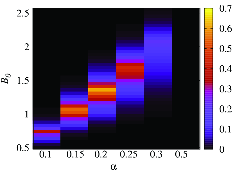
Figure 1: Density plot of the probability given by the K–S test that the CDFs of the theoretical and observed magnetic field distributions are drawn from the same population. This was generated for a range of $\alpha$ and $B_{0}$ (see text). The probability is colour-coded according to the palette shown on the right hand side of the figure. The sub-structures in this plot are caused by the discretisation of $\alpha$ and $B_{0}$.

The goal of this paper is to construct the magnetic field distribution of our synthetic sample of HFMWDs using, as a basis, the results and ideas set out by Tout et al. (2008) and Wickramasinghe et al. (2014) . If the cores of the two stars do not merge during common envelope, our assumption is that a fraction of the maximum angular momentum available at the point of the ejection of the envelope causes the shear necessary to generate the magnetic field. The non-merging case, leading to the formation of MCVs, is presented by Briggs et al. (2018, paper III). In the case of coalescing cores, a fraction of the break-up angular momentum of the resulting degenerate core provides the shear required to give rise to the strongest fields. In the following sections and in paper III we show that our models indeed show that the highest fields are generated when two stars merge and give rise to a HFMWD.

Having obtained the actual number of white dwarfs we then assign a magnetic field $B$ to each. Our prescription is that the field, generated and acquired by the white dwarf during common envelope evolution or DD merging, is proportional to the orbital angular velocity $\Omega=\displaystyle{\frac{2\pi}{P_{\rm orb}}}$ of the binary at the point the envelope is ejected and write

$$B=B_{0}\left(\frac{\Omega}{\Omega_{\rm crit}}\right)\,\mbox{G}.$$ (1)

where

$$\Omega_{\rm crit}=\sqrt{\frac{GM_{\rm WD}}{R_{\rm WD}^{3}}}=0.9\left(\frac{M_{\rm WD}}{{{\rm M}_{\odot}}}\right)^{1/2}\left(\frac{5.4\times 10^{8}}{R_{\rm WD}}\right)^{-3/2}$$ (2)

is the break-up angular velocity of a white dwarf of mass $M_{\rm WD}$ and radius $R_{\rm WD}$.

This model encapsulates the dynamo model of Wickramasinghe et al. (2014) where a seed poloidal field is amplified to a maximum that depends linearly on the initial differential rotation imparted to the white dwarf. In view of these results, here we simply assume a linear relationship between the poloidal field and the initial rotation and recalibrate the Wickramasinghe’s et al. (2014) relation between differential rotation and field using (i) a more recent set of data and (ii) results from our population synthesis calculations that provide $\Omega$ in equation (1). The quantity $B_{0}$ in equation (1) is also a parameter to be determined empirically. Different $B_{0}$’s simply shift the field distribution to lower or higher fields with no changes to the shape of the field distribution which is solely determined by the common envelope efficiency parameter $\alpha$.

For the radius of the white dwarf we use Nauenberg’s (1972) mass-radius formula

$$R_{\rm WD}=0.0112R_{\odot}\,\left[\left(\frac{M_{\rm Ch}}{M_{\rm WD}}\right)^{2/3}-\,\,\,\left(\frac{M_{\rm WD}}{M_{\rm Ch}}\right)^{2/3}\right]^{1/2},$$ (3)

where $M_{\rm{Ch}}=1.44$ M_⊙ is the Chandrasekhar limiting mass.

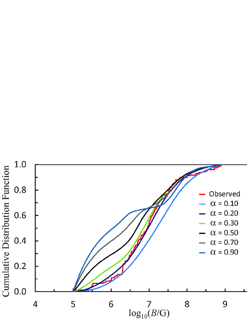
Figure 2: CDFs of observed (red) and BSE theoretical magnetic field distributions for a Galactic disc age of 9.5 Gyr and various $\alpha$.

2.2 Parameters calibration

The data set of HFMWDs is affected by many biases, even though some of the surveys that discovered them were magnitude-limited. This is because HFMWDs tend to be more massive than their non-magnetic counterparts, as first noticed by Liebert (1988), and therefore their smaller radii, as expected by equation (3), make them dimmer and so less likely to be detected. Volume-limited samples are far better, given that our synthetic population mimics a volume-limited sample, but do not include enough HFMWDs to allow us to conduct any statistically meaningful study. In this section we establish the parameter space of relevance to the observations of HFMWDs by comparing the predictions of the magnetic field distribution derived from our population synthesis calculations to the fields of HFMWDs listed in Ferrario et al. (2015). In order to achieve this goal we have employed the Kolmogorov–Smirnov (K–S) test (Press et al., 1992) to establish which combination of $B_{0}$ and $\alpha$ yield the best fit to the observed field distribution of HFMWDs. The K–S test compares the cumulative distribution functions (CDFs) of two data samples (in this case the theoretical and observed field distributions) and gives the probability $P$ that they are drawn randomly from the same population. We have calculated CDFs for seven different $\alpha$ and 44 different $B_{0}$s for each $\alpha$. If we discard all combinations of $\alpha$ and $B_{0}$ for which $P\leq 0.01$, we find $0.5\times 10^{10}\leq B_{0}/{\rm G}\leq 2.5\times 10^{10}$ and $\alpha<0.5$. We have depicted in Fig. 1 a density plot of our results. The highest probability is for $B_{0}=1.35\times 10^{10}$ G and $\alpha=0.2$. We show in Fig. 2 the theoretical CDFs for $B_{0}=1.35\times 10^{10}$ G and various $\alpha$s and the CDF of the observations of the magnetic field strengths of HFMWDs.

In the following sections we will discuss models with $B_{0}=1.35\times 10^{10}$ G and a range of $\alpha$ again noting that a different $B_{0}$ would simply move the field distribution to lower or higher fields with no change of shape. Therefore our discussion in the following sections will focus on the effects of varying $\alpha$.

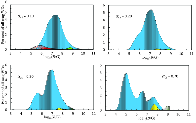
Figure 3: Theoretical magnetic field strength for a Galactic disc age of 9.5 Gyr and various $\alpha$. The histograms are superimposed, not stacked, to highlight the contribution made by each type of white dwarf to the overall distribution. The blue, red and yellow histograms represent, respectively, CO, ONe, He white dwarfs. The green histograms depict the merged DD systems.

3 Discussion of results

Fig. 3 shows the calculated magnetic field distribution and the breakdown of the WD types for $\alpha=0.1$ to $0.7$. The maximum field strength is a few $10^{9}$ G and is found mostly in systems in which the HFMWD forms either via the merging of two very compact stars on a tight orbit or through the merging of two white dwarfs after common envelope evolution (DD path). The reason for this is that these systems have very short periods and when they merge produce very strongly magnetic WDs, as expected from equation (1).

We show in Fig. 4 the theoretical magnetic field distribution of HFMWDs for $\alpha=0.1$ to $\alpha=0.7$ with the breakdown of their main formation channels, that is, their pre-common envelope progenitors. The overwhelming contributors to the HFMWD population are asymptotic giant branch (AGB) stars merging with main-sequence (MS) or deeply convective stars (CS). At low $\alpha$, systems with initially short orbital periods merge as soon as their primaries evolve off the main sequence, either whilst in the Hetzsprung’s gap or during their ascent along the red giant branch (RGB). Usually such merging events produce single stars that continue their evolution burning helium in their cores and later on, depending on the total mass of the merged star, heavier elements. Because of core nuclear burning these stars continue their evolution to eventually become single non-magnetic white dwarfs. The only observational characteristic that may distinguish them from other non-magnetic white dwarfs could be an unusual mass that does not fit any reasonable initial to final mass function associated to the stellar cluster to which they belong. On the other hand, if the RGB star has a degenerate core, as for stars with $M_{1}\leq 2.2$ M_⊙ on the ZAMS, and merges with a low-mass CS, then the resulting object is a strongly magnetic He WD. These RGB/CS merging events do occur at all $\alpha$ but their fraction is higher at large $\alpha$ owing to fewer overall merging occurrences at high envelope clearance efficiencies.

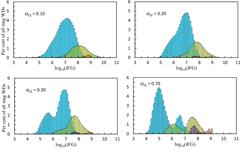
Figure 4: Theoretical magnetic field distribution of HFMWDs showing the pre-common envelope progenitors for various $\alpha$. The light blue, yellow and purple histograms represent, respectively, the AGB/MS, AGB/CS and RGB/CS merging pairs. The red histograms depict the merged DD systems.

When systems do not merge when the primary evolves on the RGB, they may merge when they undergo common envelope evolution on the AGB. In this case those binaries with the shortest orbital periods at the beginning of the common envelope evolution are those that form the highest magnetic field tail of the distribution. There are two main types of merging pairs, AGB stars merging with MS stars ($M\geq 0.7$ M_⊙) and AGB stars merging with CS ($M<0.7$ M_⊙). Each of these combinations exhibits two peaks as seen in Fig. 4 for $\alpha>0.2$, although the second peak at lower fields of the merging AGB/CS pair becomes well defined only when $\alpha=0.7$. Because AGB/MS systems have larger orbital periods at the onset of common envelope evolution, their merging gives rise to generally more massive but less magnetic white dwarfs as expected from equation (1). This is why the bulk of AGB/MS merging pairs occupy the lowest and most prominent peak near $B=10^{5.5}$ G with the secondary maximum at $B=10^{6.8}$ G. The AGB/CS merging pairs form another two peaks, one at $B=10^{6}$ G and the other at $B=10^{7.75}$ G. RGB stars merging with CS stars also form a maximum at $B=10^{7.75}$ G. The reason for the double peaks in AGB/MS and AGB/CS merging pairs is because high envelope clearance efficiencies (high $\alpha$) require more massive primaries to bring the two stars close enough together to merge during common envelope evolution. Thus, these double peaks are caused by a dearth of AGB/MS merging pairs near $B=10^{6}$ G and of AGB/CS pairs near $B=10^{7}$ G. Those systems whose orbital periods would give rise to magnetic fields in these gaps fail to merge because their initial periods are large and their primary stars are not massive enough to bring the two components close enough to merge. These double peaks are not present at low $\alpha$ because low envelope clearance efficiency always leads to tighter orbits and merging is more likely for a much wider range of initial masses and orbital periods, more effectively smearing the contributions made by specific merging pairs.

4 Comparison to observations

A prediction of our merging hypothesis for the origin of HFMWDs is that low-mass HFMWDs, mostly arising from AGB/CS merging pairs, should display fields on average stronger than those of massive HFMWDs which predominantly result from the merging of AGB/MS pairs. The HFMWDs formed through the merging of two white dwarfs (DD channel) are excluded from this prediction. These are expected to produce objects that are on average more massive, more strongly magnetic, and may be spinning much faster than most HFMWDs (e.g. RE J0317-853, Barstow et al., 1995; Ferrario et al., 1997; Vennes et al., 2003). Given the very small number of HFMWDs for which both mass and field are known, it is not possible to verify whether this trend is present in observed in HFMWDs. The problem is that it is very difficult to measure masses of HFMWDs when their field is above a few $10^{6}$ G. In the low field regime one can assume that each Zeeman component is broadened as in the zero field case. That is, the field does not influence the structure of the white dwarf’s atmosphere. Thus, the modelling of Zeeman spectra has allowed us the determination of masses and temperatures of lower field white dwarfs such as 1RXS J0823.6−2525 ($B=2.8-3.5$ MG and M=1.2 ${\rm M}_{\odot}$; Ferrario, Vennes & Wickramasinghe, 1998), PG 1658+441 ($B=3.5$ MG and M=1.31 ${\rm M}_{\odot}$; Schmidt et al., 1992; Ferrario, Vennes & Wickramasinghe, 1998) and the magnetic component of the double degenerate system NLTT 12758 ($B=3.1$ MG and $M=0.69$ ${\rm M}_{\odot}$; Kawka et al., 2017). The masses of high field objects can only be determined when their trigonometric parallax is known (e.g. Grw +70^∘8247 with $B=320\pm 20$ MG and $M=0.95\pm 0.02$ M_⊙, Greenstein, Henry & O’Connell, 1985; Wickramasinghe & Ferrario, 1988). Nevertheless, it is encouraging to see that all the most massive (near the Chandrasekhar’s limit) currently known HFMWDs do indeed possess low field strengths and that the merged DD RE J0317-853 is a strongly magnetic white dwarf. A test of our prediction of an inverse relation between field strength and mass will become possible with the release of the accurate astrometric data of a billion stars by the ESA satellite Gaia. This new set of high quality data will not only allow us to test the (non-magnetic) white dwarf mass–radius relation but will also provide us with precise mass and luminosity measurements of most of the currently known white dwarfs, including the HFMWDs (Jordan, 2007).

The theoretical distribution for $\alpha=0.2$ overlapped to the observations of HFMWDs is displayed in Fig. 5. This figure shows that the maxima of the theoretical and observed distributions occur near the same field strength with the theoretical distribution extending from $10^{5}$ G to $10^{9}$ G, as observed. The overwhelming contribution to the theoretical field distribution is from CO WDs (see Fig. 3). ONe WDs are the next most common but at much lower frequency and with field strengths $4\leq\log_{10}B/{\rm G}\leq 8$. Merged DD white dwarfs present field strengths $8\leq\log_{10}B/{\rm G}\leq 9$ at an even lower frequency than the ONe WDs. Finally, He WDs are present in very small numbers with field strengths centred at $B=10^{7.75}$ G. This is in contrast to observations of HFMWDs that show the presence of very low-mass objects (see table 1 of Ferrario et al., 2015) that the bse formalism is unable to form. This mismatch between theory and observations may be corrected through the use of, e.g., different superwind assumptions (see Han et al., 1994; Meng et al., 2008, and references therein).

We note that the models shown in Fig. 3 with $\alpha>0.2$ predict the existence of a large fraction of low-field magnetic white dwarfs with a bump appearing near $B=10^{5.5}$ G for $\alpha=0.3$. This bump shifts toward lower fields and becomes increasingly more prominent as $\alpha$ increases. For $\alpha=0.7$ this low-field hump is the most prominent feature of the magnetic field distribution. In the past suggestions were made that the incidence of magnetism in white dwarfs may be bimodal, sharply rising below $10^{5}$ G with an incidence that was predicted to be similar to or exceeding that of HFMWDs (Wickramasinghe & Ferrario, 2000). However, recent low-field spectropolarimetric surveys of white dwarfs have not found anywhere near the number of objects that had been forecast to exist in this low-field regime (Landstreet et al., 2012). Therefore, there is enough observational evidence to allow us to exclude the bimodality of the magnetic field distribution that is theoretically predicted for large $\alpha$’s.

5 Incidence of magnetism among cool white dwarfs

Because white dwarfs have very high gravities, all chemical elements heavier than hydrogen, helium and dredged-up carbon or oxygen, quickly sink to the bottom of their atmosphere. Nonetheless, up to 30 per cent of white dwarfs exhibit traces of Ca, Si, Mg, Fe, Na and other metals (DZ white dwarfs, Zuckerman et al., 2003). This metal pollution has been attributed to the steady accretion of debris from the tidal disruption of large asteroids and rocky planets (Jura, 2003) making these white dwarfs important tools for the study of the chemical composition of exosolar planets. Interestingly, the incidence of magnetism among cool ($T_{\rm eff}<8\,000$ K) DZ white dwarfs is about 13 per cent (Kawka & Vennes, 2014; Hollands et al., 2015) which is much higher than between 2 and 5 per cent in the general white dwarf population (Ferrario et al., 2015). Although our modelling does not include the merging of sub-stellar companions, we speculate that the moderately strong magnetic fields observed in metal-polluted white dwarfs ($0.5\leq B/10^{7}{\rm G}\leq 1.1$, Hollands et al., 2017) may be caused by giant gaseous planets plunging into the star. The accretion of other minor rocky bodies would then produce the observed atmospheric pollution. This mechanism could be applicable to all white dwarfs, although it is not clear what the fraction of HFMWDs that may have undergone this process is. Currently only 10 (Hollands et al., 2017) out of about 240 HFMWDs are metal-polluted. Such merging events may occur during the latest stages of AGB evolution when the outer envelope of the star engulfs the innermost planets and the drag forces exerted on them as they move through the stellar envelope cause them to drift toward the degenerate stellar core (Li et al., 1998). Whilst this mechanism is plausible, it does not explain why the incidence of magnetism is much higher among cool DZ white dwarfs. Another possibility involves close stellar encounters able to significantly disturb the orbits of outer planets and asteroid belts. Such encounters can trigger dynamical instabilities that cause the inward migration, and accretion by the white dwarf, of a massive gaseous planet and other rocky planets and asteroids. Because it takes hydrogen-rich white dwarfs with $0.5\leq M/{{\rm M}_{\odot}}\leq 1.0$ about $1.5-9$ billion years to reach effective temperatures between 5 000 and 8 000 K (Tremblay et al., 2011; Kowalski & Saumon, 2006), such stellar encounters are possible, as discussed in detail by Farihi et al. (2011) to explain the origin of the very cool ($T_{\rm eff}=5310$ K) and polluted magnetic white dwarf G77–50.

A similar explanation may be invoked to explain the high incidence of magnetism among cool white dwarfs of all types, as first reported by Liebert (1979). The study of Fabrika & Valyavin (1999) showed that whilst the incidence of magnetism among hot white dwarfs is only around 3.5 per cent, it increases above 20 per cent among cool white dwarfs. The volume-limited sample of Kawka et al. (2007) also shows a high incidence of magnetism (greater than 10 per cent) which is consistent with the fact that volume-limited samples are dominated by cooler objects. Even the Palomar-Green magnitude-limited sample study of Liebert & Bergeron (2003) shows a higher incidence of magnetism among cooler white dwarfs than hotter ones. Over the years this topic has been a cause of concern. It is difficult to think of how fields could be generated once the star has already evolved into a white dwarf because, if anything, fields decay over time. Alternatively, one could argue that the formation rate of HFMWDs was higher when the Galactic disc was younger, another hypothesis that is difficult to justify. Wickramasinghe & Ferrario (2000) and Ferrario et al. (2015) have shown that the field strength is independent of effective temperature as expected by the very long ohmic decay time scales of white dwarfs. The cumulative distribution function of the effective temperatures of the sample of HFMWDs of Ferrario et al. (2015, see their Figure 5) appears to be smooth over the full range of effective temperatures ($4\,000\leq T_{\rm eff}/{\rm K}\leq 45\,000$ K) suggesting that the birthrate of HMWDs has not altered over the age of the Galactic disc. However, the sample of HFMWDs at our disposition is neither volume nor magnitude-limited and biases easily come into play.

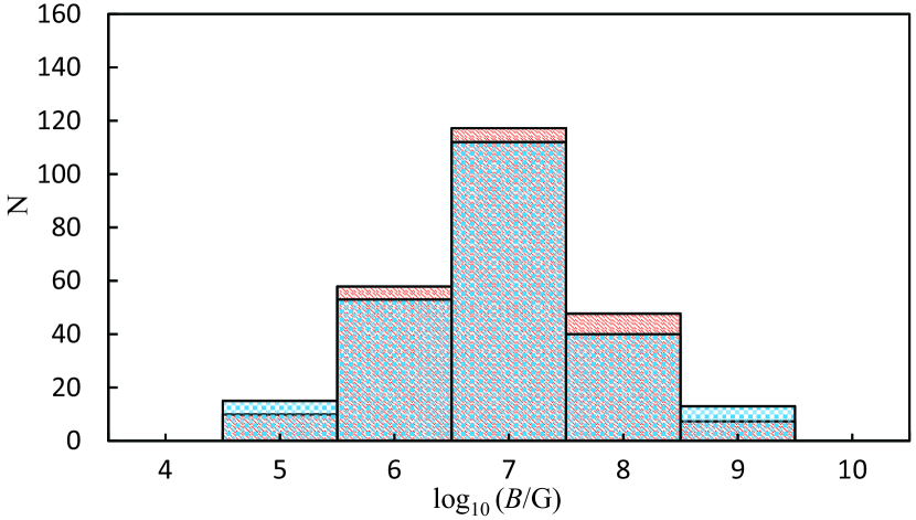
Figure 5: Theoretical field distribution for $\alpha=0.2$ of the total of the four types of HFMWDs (pink histogram) compared to the field distribution of the observed HFMWDs (blue histogram).

Thus, should a future enlarged and less biased sample of HFMWDs confirm that the incidence of magnetism among cool white dwarfs is indeed substantially higher than among hot white dwarfs, then the possibility of field generation by accretion of giant gaseous planets on to an originally non-magnetic white dwarf may provide a solution to this puzzle. Nordhaus et al. (2011) found that discs formed from tidally disrupted companions with masses in the range $0.1-500$ Jupiter masses can explain the presence of high fields in white dwarfs. Thus, the central issue is, once again, how the magnetic field can diffuse into the core of a white dwarf over an appropriate timescale. This is a key question that still needs to be quantitatively answered.

The other question concerns the likelihood for an old and presumably stable planetary system to be sufficiently perturbed to send planets inward to plunge into the white dwarf. Farihi et al. (2011) have shown that the number of close stellar encounters that can have an appreciable effect on the outer regions of a planetary system by sending objects into highly eccentric orbits is around 0.5 Gyr^-1. That is, the probability is about 50 per cent every 0.5 Gyr^-1. Considering typical cooling times between 1.5 and 9 Gyr, these close encounters become likely during the life of a white dwarf. If this hypothesis is correct, we should expect all white dwarfs hosting a large gaseous planet to develop a magnetic field at some point in their lifetime.

6 Conclusions

In paper I we discussed the evolution of HFMWDs resulting from two stellar cores (one of which is degenerate) that merge during a phase of common envelope evolution. We fitted the observed mass distribution of the HFMWDs and the incidence of magnetism among Galactic field white dwarfs and found that the HFMWDs are well reproduced by the merging hypothesis for the origin of magnetic fields if $0.1\leq\alpha\leq 0.3$. However in paper I we did not propose a prescription that would allow us to assign a magnetic field strength to each white dwarf. This task has been carried out and the results presented in this paper. We have assumed that the magnetic field attained by the core of the single coalesced star emerging from common envelope evolution is proportional to the orbital angular velocity of the binary at the point the envelope is ejected. The break-up angular velocity is the maximum that can be achieved by a compact core during a merging process and this can only be reached if the merging stars are in a very compact binary, such as a merging DD system.

In our model there are two parameters that must be empirically estimated. These are $B_{0}$, that is linked to the efficiency with which the poloidal field is regenerated by the decaying toroidal field (see Wickramasinghe et al. 2014) and the common efficiency parameter $\alpha$. A K–S test was carried out on the CDFs of the observed and theoretical field distributions for a wide range of $B_{0}$ and $\alpha$ and we found that the observed field distribution is best represented by models characterised by $B_{0}=1.35\times 10^{10}$ G and $\alpha=0.2$. Population synthesis studies of MCVs that make use of the results obtained in this paper and paper I is forthcoming and we shall show that the same $B_{0}$ can also explain observations of magnetic binaries.

We have also speculated that close stellar encounters can send a giant gaseous planet from the outer regions of a white dwarf’s planetary system into a highly eccentric orbit. The plunging of this super-Jupiter into the white dwarf can generate a magnetic field and thus provide an answer to why magnetism among cool white dwarfs, and particularly among cool DZ  white dwarfs, is higher than among hot white dwarfs.

References

- Angel et al. (1981) Angel J. R. P., Borra E. F., Landstreet J. D., 1981, ApJS, 45, 457
- Anselowitz et al. (1999) Anselowitz T., Wasatonic R., Matthews K., Sion E. M., McCook G. P., 1999, PASP, 111, 702
- Barstow et al. (1995) Barstow M.A., Jordan S., O’Donoghue D., Burleigh M. R., Napiwotzki R., Harrop-Allin M.K., 1995, MNRAS, 277, 971
- Briggs et al. (2015) Briggs G.P., Ferrario L., Tout C.A., Wickramasinghe D.T., Hurley J.R. 2015, MNRAS, 447, 1713-1723 (paper I)
- Briggs et al. (2018) Briggs G. P., Ferrario L., Tout C. A., Wickramasinghe D. T. 2018, MNRAS, submitted (paper III)
- Fabrika & Valyavin (1999) Fabrika S., Valyavin G. 1999, in ASP Conf. Ser. 169, 11th European Workshop on White Dwarfs, ed. J. E. Solheim & E. G. Meistas (San Francisco: ASP), 214
- Farihi et al. (2010) Farihi J., Barstow M. A., Redfield S., Dufour P., Hambly N. C., 2010, MNRAS, 404, 2123
- Farihi et al. (2011) Farihi J., Dufour P., Napiwotzki R., Koester D., 2011, MNRAS, 413, 2559
- Ferrario et al. (1997) Ferrario L., Vennes S., Wickramasinghe D. T., Bailey J., Christian D. J., 1997, MNRAS, 292, 205
- Ferrario (2012) Ferrario L. 2012, MNRAS, 426, 2500
- Ferrario, Vennes & Wickramasinghe (1998) Ferrario L., Vennes S. Wickramasinghe D. T. 1998, MNRASL, 299, 1
- Ferrario et al. (2015) Ferrario L., Melatos A., Zrake J. 2015a, Space Science Review, 191, 77
- Ferrario et al. (2015) Ferrario L., de Martino D., Gänsicke, B. T. 2015b, Space Science Review, 191, 111
- García-Berro et al. (2012) García-Berro E. et al., 2012, ApJ, 749, 25
- Greenstein, Henry & O’Connell (1985) Greenstein J.L., Henry R.J.W., O’Connell R.F. 1985, ApJL, 289, 25
- Han et al. (1994) Han, Z.; Podsiadlowski, P.; Eggleton, P. P., MNRAS, 270,121
- Hollands et al. (2015) Hollands M. A., Gänsicke B. T., Koester D., 2015, MNRAS, 450, 681
- Hollands et al. (2017) Hollands M. A., Koester D., Alekseev V., Herbert E. L., Gänsicke B. T., 2017, MNRAS, 467, 4970
- Hurley, Pols & Tout (2000) Hurley J. R., Pols O. R., Tout C. A., 2000, MNRAS, 315, 543
- Hurley, Tout & Pols (2002) Hurley J. R., Tout C. A., Pols O. R., 2002, MNRAS, 329, 897
- Jordan (2007) Jordan S. 2007, “15th European Workshop on White Dwarfs”, ASP Conf. Series, Vol. 372, Ed: Ralf Napiwotzki and Matthew R. Burleigh. San Francisco: ASP, 2007, p.139
- Jura (2003) Jura M., 2003, ApJ, 584, L91
- Kawka et al. (2007) Kawka A., Vennes S., Schmidt G. D., Wickramasinghe D. T., Koch R., 2007, ApJ, 654, 499
- Kawka & Vennes (2014) Kawka A., Vennes S., 2014, MNRAS, 439, L90
- Kawka et al. (2017) Kawka A. Briggs G. P., Vennes S. Ferrario L., Paunzen E., Wickramasinghe D. T. 2017, MNRAS, 466, 1127
- Kilic et al. (2017) Kilic, M., Munn, J.A., Harris, H.C., von Hippel, T., Liebert, J., Williams, K.A., Jeffery, E., DeGennaro, S., 2017, ApJ, 837, 2
- Kowalski & Saumon (2006) Kowalski P. M., Saumon D., 2006, ApJ, 651, L137
- Landstreet et al. (2012) Landstreet J. D., Bagnulo S., Valyavin G. G., Fossati L., Jordan S., Monin D., Wade G. A., 2012, A&A, 545, 30L
- Li et al. (1998) Li J., Ferrario L., Wickramasinghe D. T., 1998, ApJ, 503, L151
- Liebert (1979) Liebert J., Sion E. M., 1979, ApJ, 20, 53L
- Liebert (1988) Liebert J., 1988, PASP, 100, 1302
- Liebert & Bergeron (2003) Liebert J., Bergeron P., 2003, ApJ, 125, 348
- Liebert et al. (2005) Liebert J. et al., 2005, AJ, 129, 2376
- Liebert et al. (2015) Liebert J., Ferrario L., Wickramasinghe D. T., Smith P. S. 2015, ApJ, 804, 93L
- Meng et al. (2008) Meng X., Chen X., Han Z. 2008, A&A, 487,625
- Nauenberg (1972) Nauenberg M., 1972, ApJ 175, 417
- Nordhaus et al. (2011) Nordhaus J., Wellons S., Spiegel D. S., Metzger B. D., Blackman E. G., 2011, PNAS, 108, 3135
- Paczyński (1976) Paczyński B., 1976, in Eggleton P. P., Mitton S., Whelan J., eds, Proc. IAU Symp. 73, Structure and Evolution of Close Binary Systems, Reidel, Dordrecht, p. 75
- Potter & Tout (2010) Potter A. T., Tout C. A., 2010, MNRAS, 402,1072
- Press et al. (1992) Press W. H., Teukolsky S. A., Vetterling W. T., Flannery B. P., 1992, Numerical Recipes in Fortran 77. The Art of Scientific Computing, Cambridge Univ. Press, Cambridge
- Salpeter (1955) Salpeter E. E., 1955, ApJ, 121, 161
- Schmidt et al. (1992) Schmidt G. D., Bergeron P., Liebert J., Saffer R. A. 1992, ApJ, 394, 603
- Schmidt et al. (2001) Schmidt G. D., Vennes S., Wickramasinghe D. T., Ferrario L., 2001, MNRAS, 328, 203
- Sion et al. (1988) Sion E. M., Fritz M., McMullin J. P., Lallo M. D., 1988, AJ, 96, 251
- Sion et al. (2009) Sion E. M., Holberg J. B., Oswalt T. D., McCook G. P., Wasatonic R., 2009, AJ, 138, 1681S
- Tout et al. (2004) Tout C. A., Wickramasinghe D. T., Ferrario L., 2004, MNRAS, 355, L13
- Tout et al. (2008) Tout C. A., Wickramasinghe D. T., Liebert J., Ferrario L., Pringle J. E., 2008, MNRAS, 387, 897
- Tremblay et al. (2011) Tremblay P.-E., Bergeron P., Gianninas A., 2011, ApJ, 730, 128
- Vennes et al. (2003) Vennes S., Schmidt G. D., Ferrario L., Christian D. J., Wickramasinghe D. T., Kawka A. 2003,ApJ, 593, 1040
- Wickramasinghe & Ferrario (1988) Wickramasinghe D.T., Ferrario L. 1988, ApJ, 327, 222
- Wickramasinghe & Ferrario (2000) Wickramasinghe D. T., Ferrario L., 2000, PASP, 112, 873
- Wickramasinghe & Ferrario (2005) Wickramasinghe D. T., Ferrario L., 2005, MNRAS, 356, 615
- Wickramasinghe, Tout & Ferrario (2014) Wickramasinghe D. T., Tout C. A., Ferrario L., 2014, MNRAS, 437, 675
- Zuckerman et al. (2003) Zuckerman B., Koester D., Reid I. N., H¨unsch M., 2003, ApJ, 596, 477