Near-Lossless Deep Feature Compression for Collaborative Intelligence

Abstract

Collaborative intelligence is a new paradigm for efficient deployment of deep neural networks across the mobile-cloud infrastructure. By dividing the network between the mobile and the cloud, it is possible to distribute the computational workload such that the overall energy and/or latency of the system is minimized. However, this necessitates sending deep feature data from the mobile to the cloud in order to perform inference. In this work, we examine the differences between the deep feature data and natural image data, and propose a simple and effective near-lossless deep feature compressor. The proposed method achieves up to 5% bit rate reduction compared to HEVC-Intra and even more against other popular image codecs. Finally, we suggest an approach for reconstructing the input image from compressed deep features that could serve to supplement the inference performed by the deep model.

I Introduction

Recent advances in deep neural networks (DNNs) are making various artificial intelligence (AI)-enabled applications feasible: intelligent surveillance cameras, automated personal assistants, self-driving cars, unmanned aerial vehicles, and so on [1]. A common deployment strategy for AI-based applications on mobile devices is to have the AI model running in the cloud while the terminus device sends its data to it for inference, and receives the results back. In certain cases, small models may run on the terminus device, but the large models that form the backbone of most AI-enabled systems are too power hungry to run on a mobile device.

A recent study [2] proposed a new deployment paradigm called collaborative intelligence, whereby a deep model is split between the mobile and the cloud. Extensive experiments under various hardware configurations and wireless connectivity modes revealed that the optimal operating point in terms of energy consumption and/or computational latency involves splitting the model, usually at a point deep in the network. Today’s common solutions, where the model sits fully in the cloud or fully at the mobile, were found to be rarely (if ever) optimal. Another recent study [3] extended the notion of collaborative intelligence to model training as well. In this case, data flows both ways: from the cloud to the mobile during back-propagation in training, and from the mobile to the cloud during forward passes in training, as well as inference.

In these early studies, the issue of compression for the purpose of data transfer between the mobile and the cloud was not studied in detail. In fact, [2] assumed the transfer of raw 32-bit floating point feature values, which is rather wasteful. The work in [3] included 8-bit quantization followed by PNG coding of quantized feature maps. The work in [4] was the first to study lossy compression of deep feature data based on HEVC intra coding, in the context of a recent deep model for object detection [5]. They noted the degradation of detection performance with increased compression levels and proposed compression-augmented training to minimize this loss by producing a model that is more robust to quantization noise in feature values. However, this is still a sub-optimal solution, because the codec employed is highly complex [6] and optimized for natural scene compression rather than deep feature compression.

A related work [7] presented semantic image compression by encoding deep features and then reconstructing the input image from them. The compression was based on uniform quantization followed by context-based adaptive arithmetic coding (CABAC) from H.264 [8]. This work was positioned as an image codec that preserves semantic information for image classification, rather than a tool for collaborative intelligence, but the similarities are evident. Although the overall compression efficiency of this approach was somewhat lower than JPEG and JPEG2000, the authors argued that the benefits lie in better preservation of semantic information.

With a view towards collaborative intelligence, in this work we propose a simple and effective near-lossless compression method tailored to deep feature data. We focus on deep models for object detection [5] and image classification [9], but the approach is applicable to other deep models as well. In Section II we analyze feature data from the two models under study, and note some of the statistical differences between deep feature data and input image data. This analysis informs the design of the proposed compression scheme in Section III. Furthermore, we demonstrate the capability of reconstructing the input image from compressed deep features in Section IV by constructing and training a mirror model of front-end layers. Experimental results and conclusions are presented in Sections V and VI, respectively.

II Deep feature data analysis

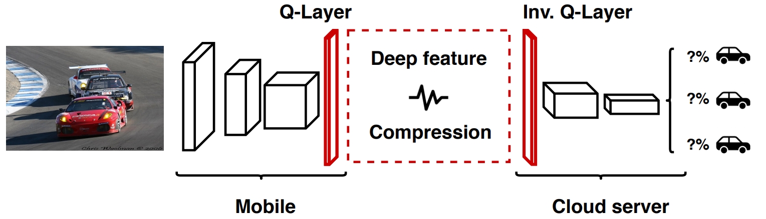
Figure 1: Collaborative intelligence approach with deep feature compression

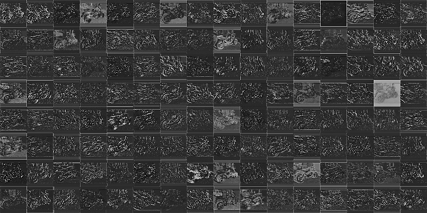
(a)

(b)

(c)

(d)

(e)

(f)

Figure 2: Quantized deep features (enhanced for visualization purposes) from YOLOv2 [5] and VGG16 [9] at various points in the network. Top row: (a) seventh (b) eleventh and (c) seventeenth layer in YOLOv2. Bottom row: (d) sixth (e) tenth and (f) fourteenth layer in VGG16.

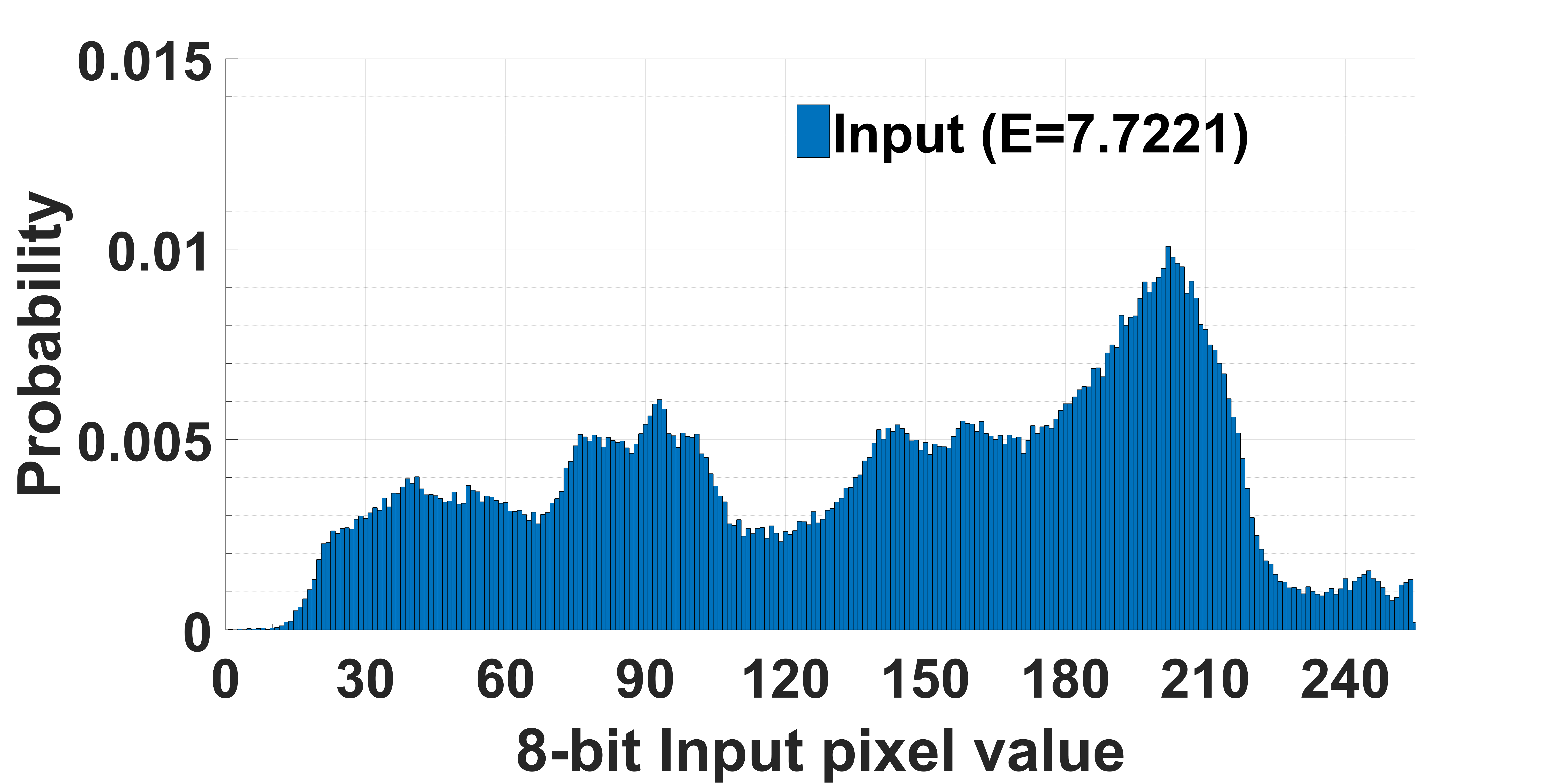
(a)

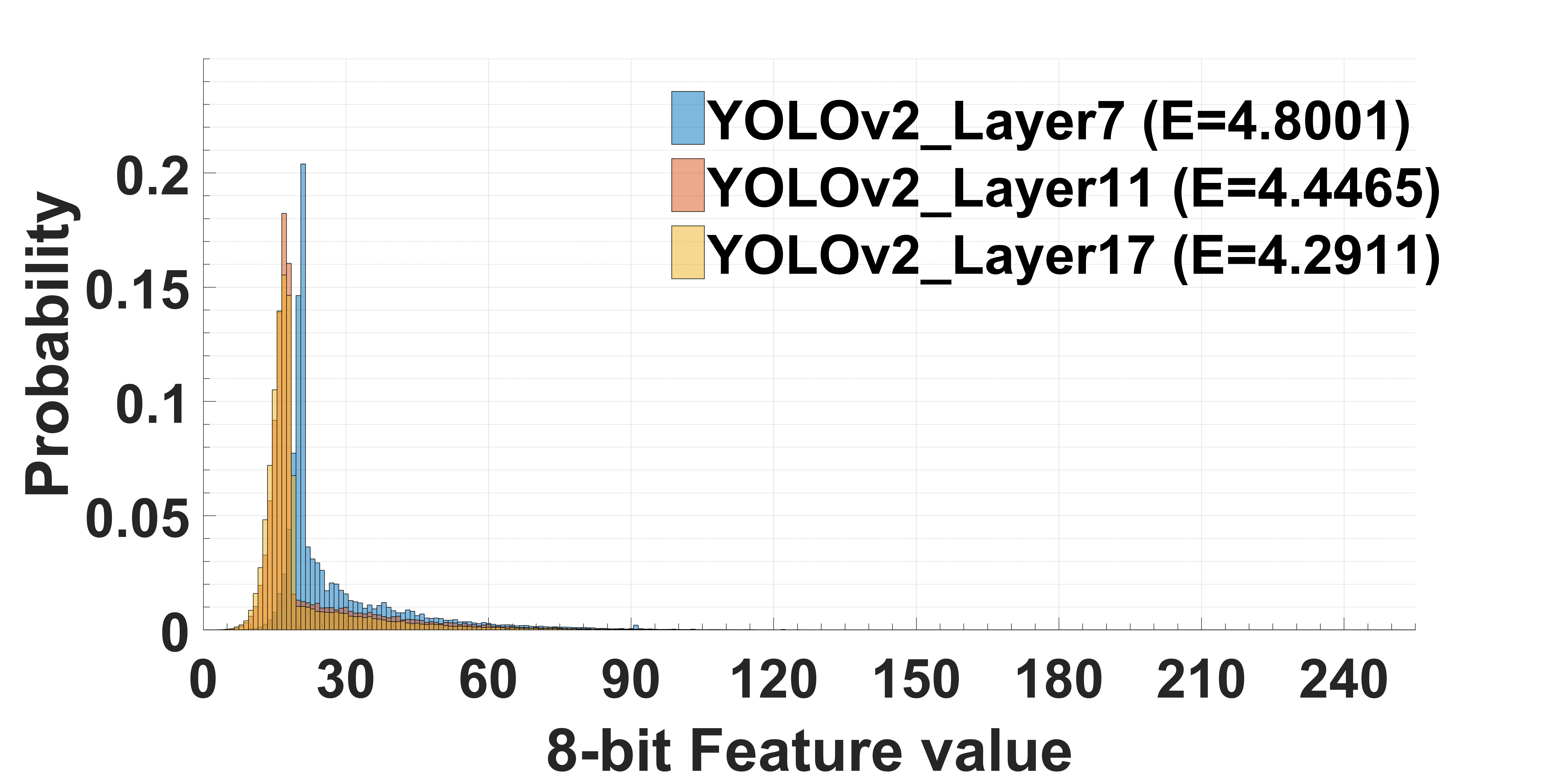
(b)

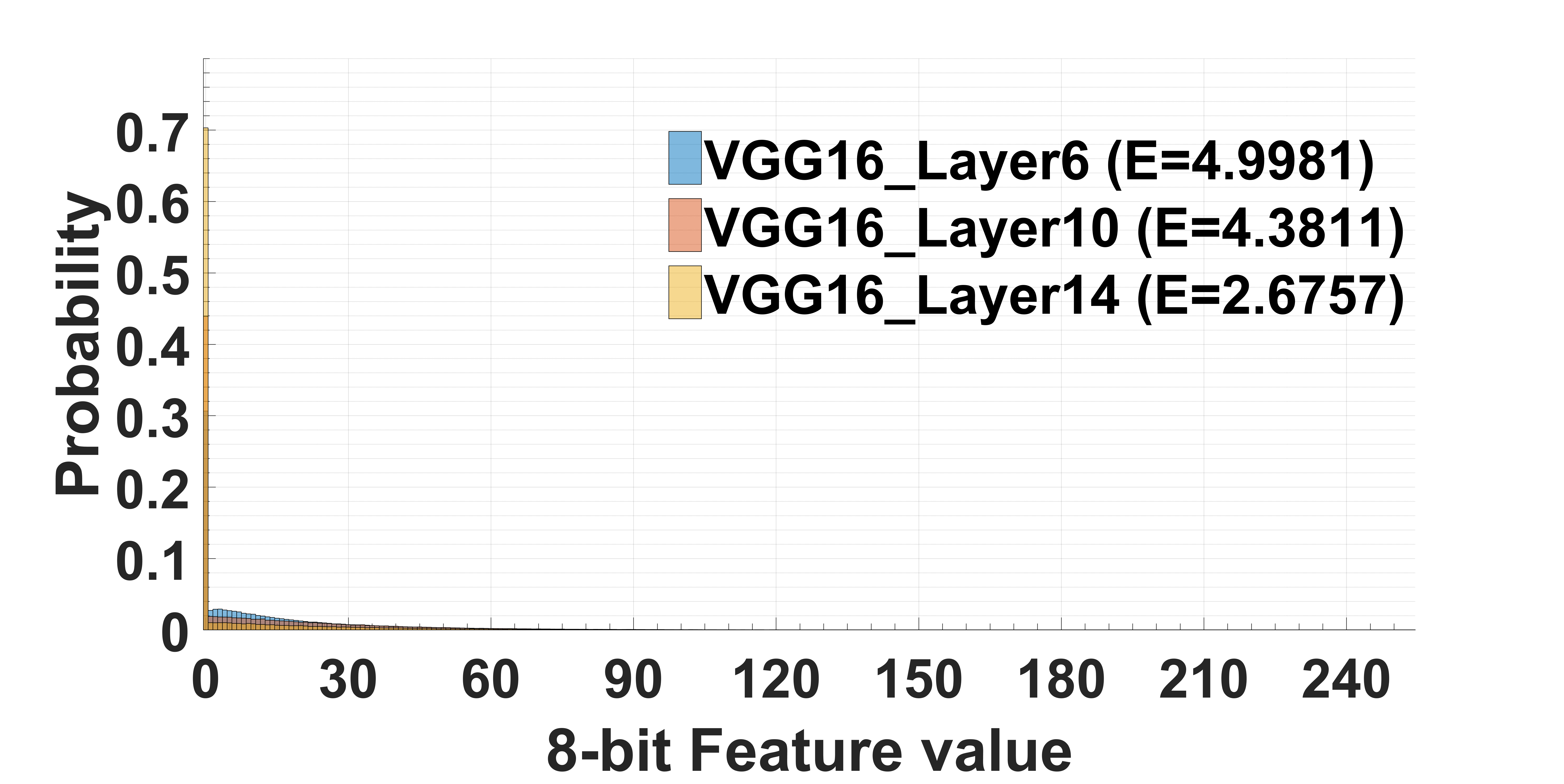
(c)

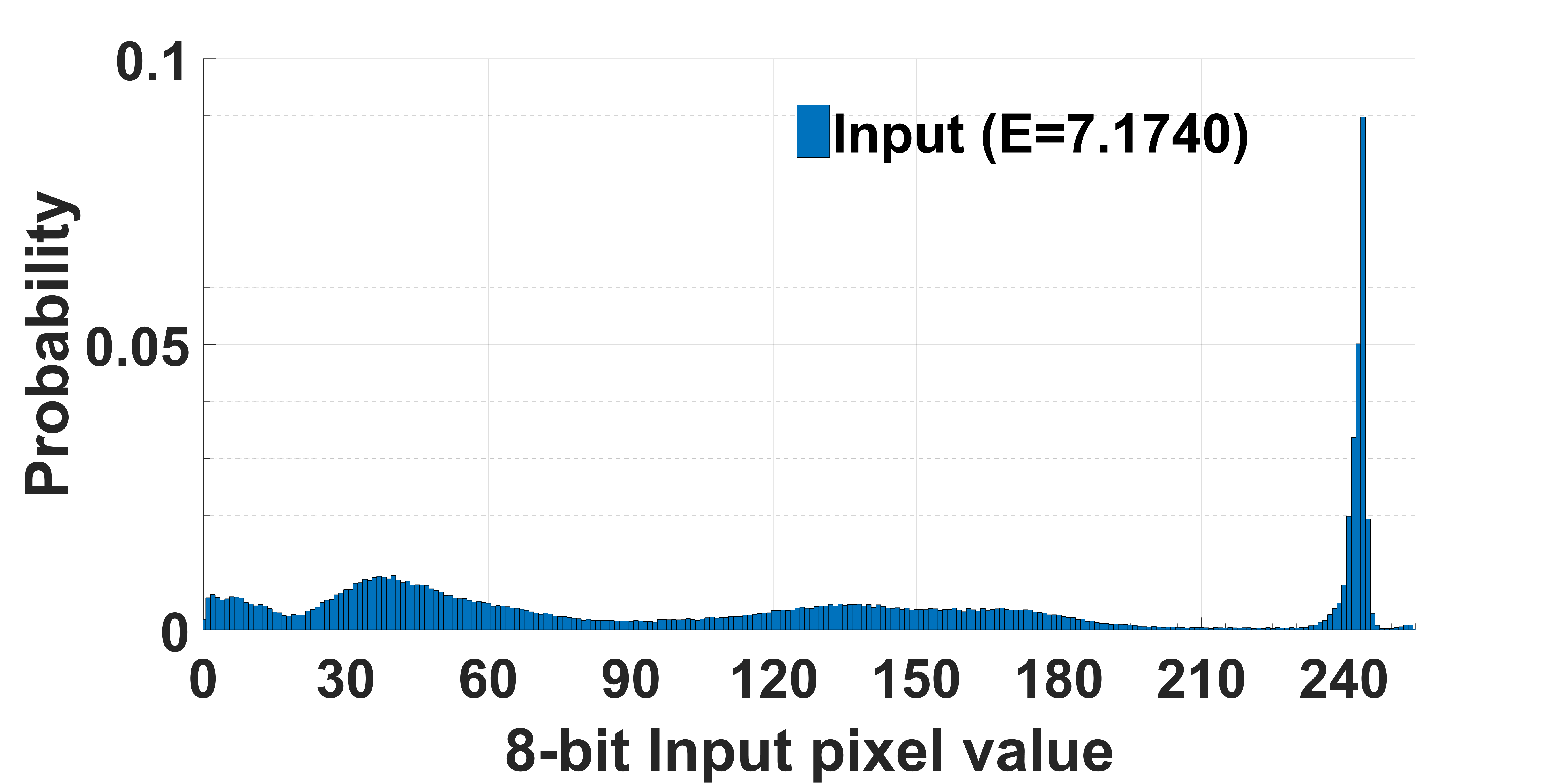
(d)

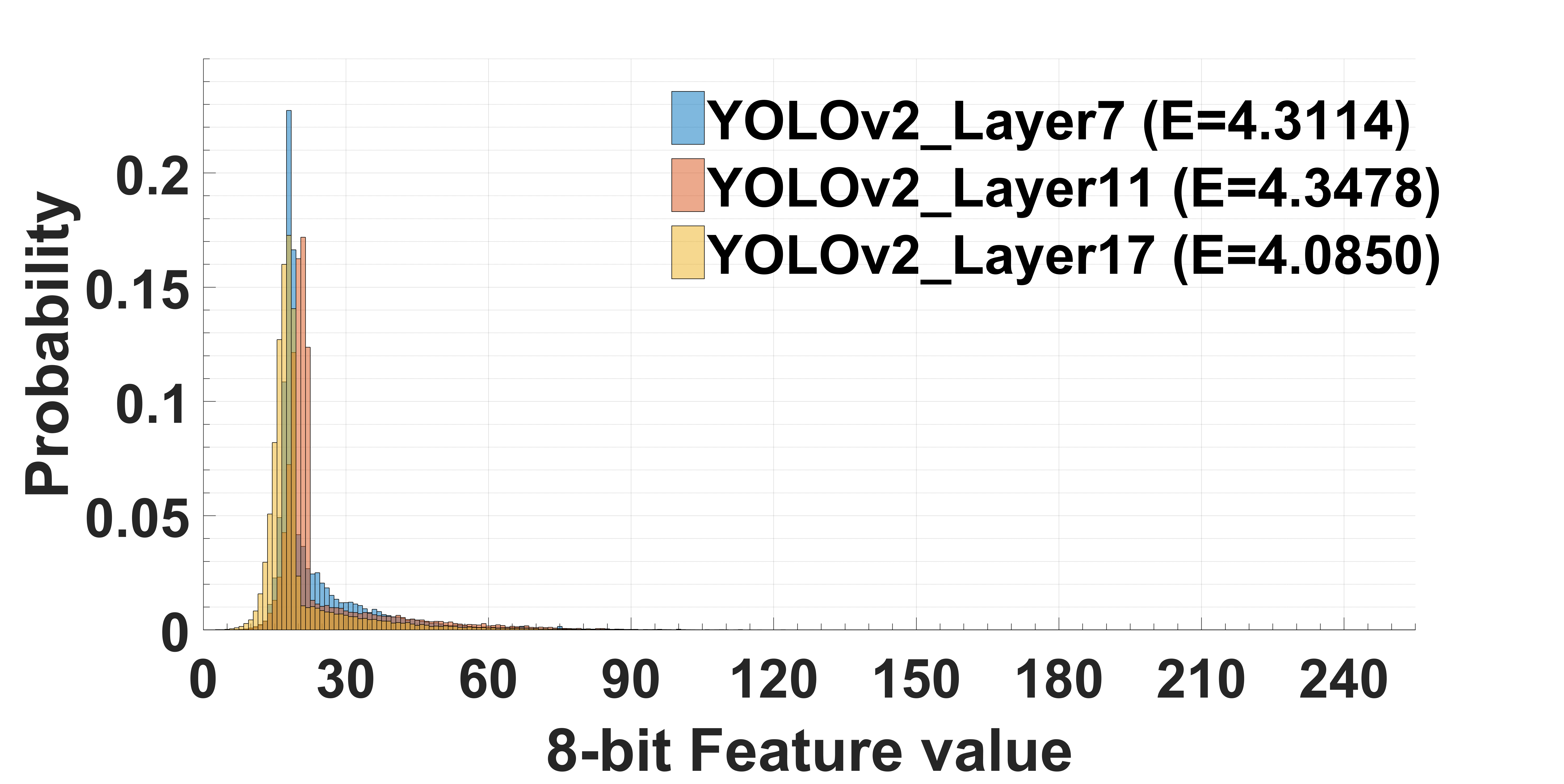
(e)

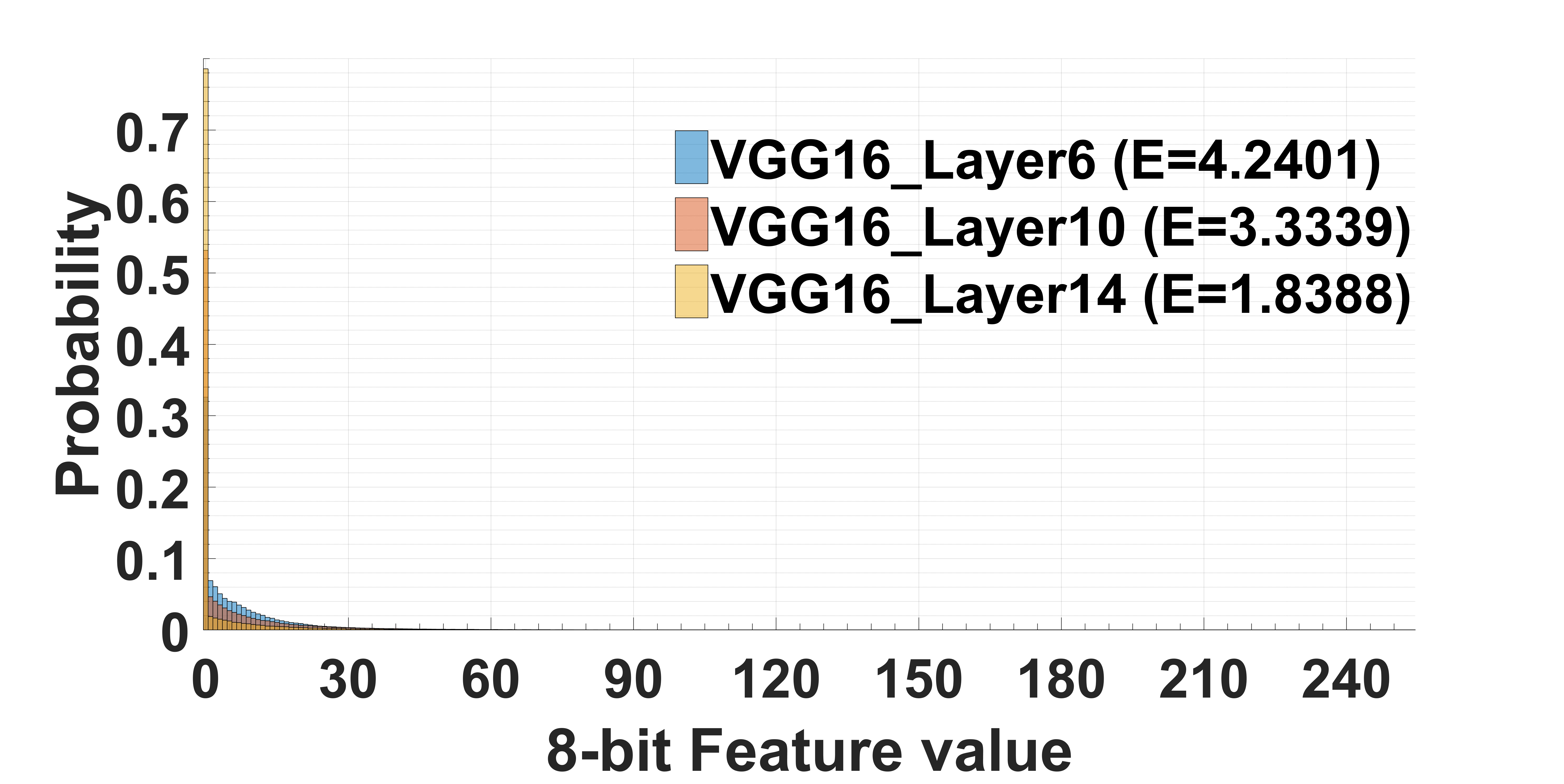
(f)

Figure 3: (a) and (d) are histograms of pixel values of two input images, (b) and (e) are histograms of the quantized output of the seventh, eleventh and seventeenth layer of YOLOv2, while (c) and (f) are histograms of the quantized output of the sixth, tenth and fourteenth layer of VGG16. Corresponding entropies (E, in bits) are indicated in the plots.

Fig. 1 shows the basic setup for collaborative intelligence, where the feature data produced by the initial layers of the deep model are compressed and sent to the cloud for further processing. The efficiency of this approach lies in the fact that for many deep models based on convolutional neural networks (CNNs), the feature data volume (i.e., the total number of feature values) decreases as we move deeper into the network [2, 3, 4]. Feature values are typically quantized using an $n$-bit uniform quantizer (Q-layer in Fig. 1) prior to lossless [3] or lossy [4] compression.

$$\widetilde{\mathbf{V}}=\textup{round}\left(\frac{\mathbf{V}-\min(\mathbf{V})}{\max(\mathbf{V})-\min(\mathbf{V})}\cdot(2^{n}-1)\right)$$ (1)

where $\mathbf{V}\in\mathbb{R}^{N\times M\times C}$ is the feature tensor with $N$ rows, $M$ columns, and $C$ channels at the point of split, $\widetilde{\mathbf{V}}$ is the quantized feature tensor, and $\min(\mathbf{V})$ and $\max(\mathbf{V})$ are the minimum and maximum value in $\mathbf{V}$, respectively. In the studies performed so far [3, 4, 7], this uniform $n$-bit quantization was shown to have negligible effect on image classification and object detection accuracy, for $n\geq 6$. For this reason, when such uniform quantizer is followed up by a lossless encoder, we refer to the resulting approach as near-lossless compression. In this work, the Q-layer performs uniform $8$-bit quantization. Note that $\min(\mathbf{V})$ and $\max(\mathbf{V})$ need to be transferred to the cloud for the inverse Q process.

The quantized features $\widetilde{\mathbf{V}}$ are rearranged in a tiled image, as shown in Fig. 2. With $C$ channels, we place

$$2^{\textup{ceil}\left(\frac{1}{2}\log_{2}C\right)}\qquad\text{and}\qquad 2^{\textup{floor}\left(\frac{1}{2}\log_{2}C\right)}$$ (2)

feature channels (tiles) width-wise and height-wise, respectively. Here, ceil$(\cdot)$ and floor$(\cdot)$ represent ceiling and flooring to the nearest integer, respectively.

Fig. 2 shows the tiled quantized features obtained from YOLOv2 [5] and VGG16 [9] with default weights for the same input image. For each model, three layers are selected (max-pooling layers in all cases) where the resulting feature volume is of comparable size between the two models. We see that, qualitatively, the features are different between the two models, which is not surprising considering that they were trained for different purposes. There are several tiles that still contain somewhat interpretable structures in Fig. 2(a) and (d), but the features become more abstract as we move towards deeper layers (b), (c), (e) and (f). Both sets of features also differ significantly from natural images.

Fig. 3 shows pixel and feature histograms for two different input images. As shown in Fig. 3(a) and (d), which present the luma histograms of input images, pixel intensities in natural images tend to be distributed over the entire range 0-255. In these two input images, no pixel value has a probability above $0.1$. Meanwhile, histograms of quantized feature values from all channels in Fig. 3(b), (c), (e), and (f) are much more concentrated, and they tend to become more concentrated as we move deeper into the network. Entropy values indicated in figure legends confirm this quantitatively.

While feature value concentration occurs in both YOLOv2 and VGG16, it is interesting that the concentration points in these two models are different. VGG16 uses Rectified Linear Unit (ReLU) activations [10], which are lower-bounded by zero, and the resulting features values concentrate near zero. On the other hand, YOLOv2 uses leaky ReLU activations [10], which admit negative values. Hence, prior to quantization, feature values concentrate near zero, but negative feature values exist (i.e., $\min(\mathbf{V})<0$). After quantization (1), zero gets mapped to a small positive value (usually 15-25), so the concentration point of quantized features is away from zero.

TABLE I: Similarity of pixel/feature values with spatial neighbors and most frequent values

		$\textup{AD}_{m}^{2}$	$\textup{AD}_{l}^{2}$	$\textup{AD}_{t}^{2}$	$\textup{AD}_{tl}^{2}$	$\textup{AD}_{bl}^{2}$	$\textup{AD}_{tr}^{2}$	none
Input image		22.06%	26.19%	10.77%	4.83%	4.23%	3.27%	28.65%
YOLOv2	L7	67.59%	9.75%	3.65%	1.27%	1.20%	1.02%	15.52%
	L11	73.81%	5.80%	2.34%	0.81%	0.80%	0.71%	15.73%
	L17	83.63%	1.12%	0.30%	0.28%	0.28%	0.25%	14.14%
VGG16	L6	64.49%	6.69%	4.30%	1.86%	1.82%	1.56%	19.28%
	L10	69.62%	3.75%	2.72%	1.42%	1.41%	1.26%	19.82%
	L14	83.68%	1.12%	0.84%	0.45%	0.46%	0.43%	13.02%

Next we examine spatial statistics. Specifically, we look at the similarity between the current pixel and its neighbors: left ($l$), top ($t$), top-left ($tl$), bottom-left ($bl$), and top-right ($tr$). We also look at the similarity with the 8 most frequent values in a given histogram: $m_{i},i=0,1,...7$. To capture the similarity, we consider indicators $\textup{AD}_{k}^{T}$ for a given threshold $T$, where $k\in\left\{m,l,t,tl,bl,tr\right\}$. $\textup{AD}_{m}^{T}$ is incremented if the absolute difference between the current pixel/feature value $x$ and any (one or more) of the $m_{i}$ values is less than $T$: $|x-m_{i}|<T$ for any $i$. If $|x-m_{i}|\geq T$ for all $i$, then we test the similarity with $k\in\left\{l,t,tl,bl,tr\right\}$, in that order. If $|x-k|<T$, $\textup{AD}_{k}^{T}$ is incremented and we move to the next pixel/feature value. Table I shows $\textup{AD}_{k}^{T}$ for $T=2$, expressed as percentages. The results were obtained on the 2510 images from the VOC2007 dataset [11]. Compared to the natural image statistics (second row in the table), we note that feature values exhibit much more similarity with the most frequent values ($\textup{AD}_{m}^{2}$), and much less similarity with spatial neighbors ($\textup{AD}_{k}^{2}$, for $k\in\left\{l,t,tl,bl,tr\right\}$). This trend increases as we move deeper into the network. Hence, one cannot expect that natural image codecs, which place strong emphasis on spatial redundancy, would be optimal for encoding deep feature data – new approaches are needed for this purpose.

III Deep feature compression

Fig. 4 shows the proposed compression framework for deep features in collaborative intelligence applications. In the cloud, deep features are decoded and used for inference. They can also optionally be used for input reconstruction, as discussed in Section IV.

Before coding the quantized feature data, the following parameters are encoded directly using fixed-length coding: dimensions of the feature tensor, $\min(\mathbf{V})$ and $\max(\mathbf{V})$ (32-bit each) and the eight most frequent feature values, $m_{i}$ for $i=0,1,...7$. The set of $\{m_{i}\}$ is obtained over the entire quantized feature tensor. A vector of these values, $\mathbf{p}=(p_{0},p_{1},...,p_{7})$, is referred to as the palette vector.

Initially, the palette vector is sorted according to the frequency of these values in the first tile, so that $p_{0}$ is the most frequent of the $m_{i}$’s in the first tile, $p_{1}$ is the next most frequent, etc. As we move to other tiles, the palette vector $\mathbf{p}=(p_{0},p_{1},...,p_{7})$ is re-sorted according to the frequency of occurrence of $m_{i}$’s up to the previously coded tile, so that $p_{0}$ is the most frequent $m_{i}$ up to that point, and so on. At the tile boundary, once $\mathbf{p}$ is updated, one element of $\mathbf{p}$ is chosen to minimize the mean absolute difference (MAD) from the feature values in the to-be-coded tile. Its index is found as

$$j^{*}=\operatorname*{arg\,min}_{0\leq j\leq 7}\sum_{i}{|x_{i}-p_{j}|}$$ (3)

where $i$ goes over all locations in the tile. Once $j^{*}$ is found, it is encoded using the truncated 8-symbol unary code [12] shown in Table II.

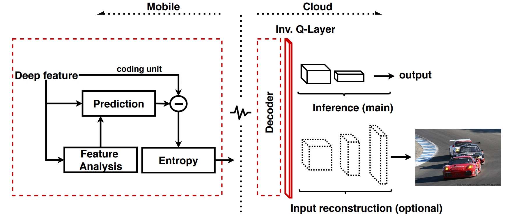
Figure 4: Proposed deep feature compression for collaborative intelligence

TABLE II: Unary code for the palette index

Index $j^{*}$	Codeword	Index $j^{*}$	Codeword
$0$	1	$4$	11110
$1$	10	$5$	111110
$2$	110	$6$	1111110
$3$	1110	$7$	1111111

Every 4$\times$4 block of feature values is predicted using one of five modes: palette (Pal), horizontal (Hor), vertical (Ver), and two filter modes (Fil). In the Pal mode, all values in the block are predicted using $p_{j^{*}}$. In Hor/Ver modes, the immediate left/top value is used as a predictor, as indicated in Fig. 5. If the block is at the left (top) boundary, $p_{j^{*}}$ is used as the left (top) value. The two Fil modes are based on 3-tap filters with coefficients $[3,7,22]/32$ or $[14,0,18]/32$ [13], and use the top-left, top, and left feature values to predict the current value. Again, at the boundaries, the unavailable values are replaced by $p_{j^{*}}$.

Prediction mode decision is based on the number of bits required for coding the residual, with the best mode being the one that requires least bits. In order to minimize the bits needed to specify the prediction mode, we exploit the most probable mode (mpm) method [14], where mpm is derived from the previously-coded left, top-left and top blocks’ prediction modes. The most frequently used mode among them is considered the mpm. If the current block’s mode is the same as mpm, bit 1 is coded by CABAC [15] to indicate it. Otherwise, bit 0 is coded, followed by two bits to indicate the mode.

Prediction residuals for each $4\times 4$ block are coded by CABAC. The first bit is the SKIP indicator. If the residual is all-zero, the SKIP indicator is set to 1 and the encoder moves to the next block. Otherwise, the SKIP indicator is set to 0 and residuals are coded using one of three scan orders: horizontal, vertical, and zig-zag. For the Ver (Hor) prediction mode, vertical (horizontal) scan order is used. Other modes use the zig-zag scan order. Locations of non-zero residuals are first indicated by binarizing the scanned block, with 1’s placed at the locations of non-zero residuals and 0’s placed elsewhere. This binary vector is coded using CABAC. Finally, the non-zero residual values are coded in a manner similar to HEVC [15]: values larger than 1 or 2 are flagged, the flags are CABAC-coded, and the non-flagged values are binarized using exponential Golomb-Rice coding, then coded by CABAC.

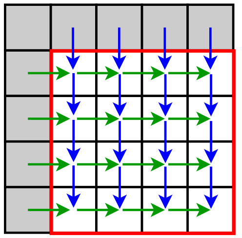
Figure 5: Illustration of Hor (green) and Ver (blue) prediction modes for the 4$\times$4 block (red). Shaded regions are neighbouring feature values.

IV Input reconstruction

Although the primary goal of collaborative intelligence is efficient inference, in some cases it may be desirable to also have the input image available in the cloud. For example, if the model detects an object of interest based on the features that were transmitted to the cloud, it might be useful to have the whole input image, which can then be stored or further processed in the cloud. The straightforward way is to simply send the whole input image from the mobile to the cloud, but this is not necessary, since a good approximation to the input image can be reconstructed from the transmitted features.

To demonstrate this, we construct a mirror model, indicated in the bottom right of Fig. 4, based on the the network in the mobile. Specifically, given the network in the mobile, the mirror model consists of the same number of layers, but in reverse order: convolutional layers from the mobile network are mapped to the convolutional layers with the same kernel size in the mirror model, while max-pooling layers from mobile network are mapped to up-sampling layers.

The goal of the mirror model is to reconstruct the input image from the deep features transmitted to the cloud. We train the mirror model using a loss function that combines structural similarity (SSIM) [16] and mean square error (MSE) between the input and the reconstructed image, as

$$L=\lambda_{1}\cdot(1-\textup{SSIM})+\lambda_{2}\cdot\textup{MSE}$$ (4)

We used $\lambda_{1}=0.6$ and $\lambda_{2}=1$. The mirror model is trained from scratch using the Adam optimizer [17] with the initial learning rate of $10^{-4}$. A total of 16,551 images from [11] and [18] are employed for training the model, with 20% randomly selected as validation data and the remaining 80% used for training. The test set consists of another 4,952 images from [11]. The maximum number of epochs is set to 50 and batch size to 32. The training stops when the validation loss starts increasing.

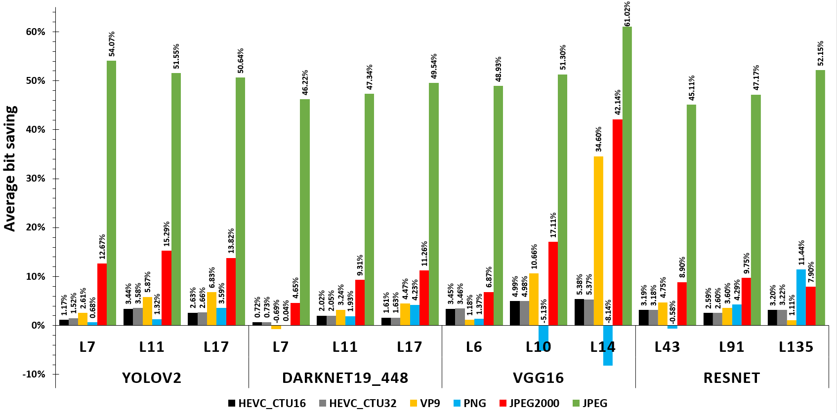
Figure 6: Comparison of average bits saving for the three different deep features from each network against conventional compression algorithms

V Experiments

The proposed deep feature compression was tested on four deep models: YOLOv2 [5], Darknet19_448 [19], VGG16 [9] and ResNet [20]. YOLOv2 is a state-of-the-art object detector, while other models are used for image classification. Table III shows the size of the feature tensor at the output of three layers from each of the models, along with the dimensions of the feature matrix after tiling. For testing compression of YOLOv2 features we used 4,952 images from VOC2007 [11], and for other models we used 50,000 images from ImageNet [21].

Deep features produced by the various models were compressed using the proposed method, as well as the lossless versions of HEVC [22], VP9, PNG, JPEG2000 and JPEG. For HEVC, we followed common test conditions [23] associated with lossless coding, while changing the largest coding unit size, also known as CTU, to 32$\times$32 and 16$\times$16.

As usual, evaluation of lossless coding is based on the number of bits used. Fig. 6 shows the average bit difference between the proposed method and each of the five competing methods, on the image datasets described above. Positive values mean that the competing method uses more bits than the proposed one. As seen in the figure, HEVC (with both CTU sizes) needs 0.7-3.0% more bits than the proposed method in most cases, and up to 5% more for the tenth and fourteenth layer of VGG16. VP9 also uses more bits than the proposed method (up to 34% more in the fourtenth layer of VGG16), except for the seventh layer of the Darkent19_448 where it uses 0.96% fewer bits. PNG turns out to be a very good codec for deep feature data. While it uses more bits than the proposed method in most cases, it needs up to 9% fewer bits in the fourteenth layer of VGG16. Both JPEG2000 and JPEG require considerably more bits than other codecs. Compared to the proposed method, JPEG2000 needs up to 45% more bits and JPEG needs up to 61% more bits. Also, Table IV shows the average mode selection percentage for each model in the study. As observed in Table IV, Pal is the most frequently used prediction mode in each of the four models, accounting for 35-58% of predictions.

TABLE III: Dimensions of feature tensors and feature matrices at three different layers of each of the models in the study.

Model	Layer	Feature tensor	Feature matrix
YOLOv2	L7	128$\times$52$\times$52	832$\times$416
	L11	256$\times$26$\times$26	416$\times$416
	L17	512$\times$13$\times$13	416$\times$208
Darknet19_448	L7	128$\times$56$\times$56	896$\times$448
	L11	256$\times$28$\times$28	448$\times$448
	L17	512$\times$14$\times$14	448$\times$224
VGG16	L6	128$\times$56$\times$56	896$\times$448
	L10	256$\times$28$\times$28	448$\times$448
	L14	512$\times$14$\times$14	448$\times$224
ResNet	L43	128$\times$32$\times$32	512$\times$256
	L91	256$\times$16$\times$16	256$\times$256
	L135	256$\times$16$\times$16	256$\times$256

TABLE IV: Average mode selection percentage for each model

Model	Hor	Ver	Pal	Fil1	Fil2
YOLOv2	31.67	18.10	35.02	9.95	5.26
Darknet19_448	13.56	13.91	58.06	9.21	5.26
VGG16	25.14	19.92	42.93	7.83	4.18
ResNet	17.25	12.80	51.42	14.13	4.40

Finally, we demonstrate input reconstruction from the features generated at the seventh, eleventh and seventeenth layer of YOLOv2. Hence, three mirror models are trained for reconstruction, one for each set of features. Table V shows the average Peak Signal to Noise Ratio (PSNR, in dB) and SSIM, along with standard deviations, over the test set. As seen in the table, the deeper the layer from which features are extracted, the more difficult is the input reconstruction, since more information gets lost in max-pooling layers. Visual results, shown in Fig. 7, look somewhat better than what is suggested by quantitative results in Table V. The first row shows the original input images, while the remaining rows show reconstructed images from the seventh, eleventh and seventeenth layer, in that order. Reconstructions from the seventh layer look reasonably good compared to the original images. However, reconstructions from deeper layers start to lose important details.

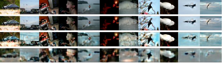
Figure 7: Top row: original input images. Other rows: reconstructed images from the seventh, eleventh, and seventeenth layer of YOLOv2.

TABLE V: Comparison of PSNR & SSIM index for the reconstructed input images compared to original inputs.

		PSNR		SSIM
		Avg.	Std.	Avg.	Std.
L7	Y	23.8633	2.8674	0.7042	0.1107
	U	35.8363	3.8942	0.9411	0.0344
	V	33.0488	4.1624	0.9160	0.0452
L11	Y	17.5348	1.7231	0.4743	0.1319
	U	30.7260	2.6935	0.9106	0.0466
	V	27.6556	3.1462	0.8645	0.0613
L17	Y	14.2898	1.7578	0.4044	0.1367
	U	28.6288	3.5730	0.9072	0.0505
	V	25.8074	3.9733	0.8560	0.0648

VI Conclusion

In this study, we examined the characteristics of deep feature data and proposed a simple and effective method for near-lossless deep feature compression. The proposed method outperforms state-of-the-art image codec in this regard. We also demonstrated input image reconstruction from deep feature data by constructing and training a mirror model. Future work will involve the development of lossy compression schemes for deep feature data.

References

- [1] A. Poniszewska-Maranda, D. Kaczmarek, N. Kryvinska, and F. Xhafa, “Endowing iot devices with intelligent services,” in Proc. Int. Conf. Emerging Internetworking, Data & Web Technol., 2018, pp. 359–370.
- [2] Y. Kang, J. Hauswald, C. Gao, A. Rovinski, T. Mudge, J. Mars, and L. Tang, “Neurosurgeon: Collaborative intelligence between the cloud and mobile edge,” in Proc. 22nd ACM Int. Conf. Arch. Support Programming Languages and Operating Syst., 2017, pp. 615–629.
- [3] A. E. Eshratifar, M. S. Abrishami, and M. Pedram, “JointDNN: an efficient training and inference engine for intelligent mobile cloud computing services,” arXiv preprint arXiv:1801.08618, 2018.
- [4] H. Choi and I. V. Bajić, “Deep feature compression for collaborative object detection,” in Proc. IEEE ICIP’18, 2018, to appear.
- [5] J. Redmon and A. Farhadi, “YOLO9000: better, faster, stronger,” in Proc. IEEE CVPR’17, Jul. 2017, pp. 6517–6525.
- [6] F. Bossen, B. Bross, K. Suhring, and D. Flynn, “HEVC complexity and implementation analysis,” IEEE Trans. Circuits Syst. Video Technol., vol. 22, pp. 1685–1696, Dec. 2012.
- [7] S. Luo, Y. Yang, and M. Song, “DeepSIC: Deep semantic image compression,” arXiv preprint arXiv:1801.09468, 2018.
- [8] D. Marpe, H. Schwarz, and T. Wiegand, “Context-based adaptive binary arithmetic coding in the H.264/AVC video compression standard,” IEEE Trans. Circuits Syst. Video Technol., vol. 13, pp. 620–636, July 2003.
- [9] A. Zisserman K. Simonyan, “Very deep convolutional networks for large-scale image recognition,” arXiv preprint arXiv:1409.1556, 2014.
- [10] G. Ian, B. Yoshua, and C. Aaron, Deep Learning, MIT Press, 2016.
- [11] M. Everingham, L. Van Gool, C. K. I. Williams, J. Winn, and A. Zisserman, “The PASCAL Visual Object Classes Challenge 2007 (VOC2007) Results,” http://host.robots.ox.ac.uk/pascal/VOC/voc2007/.
- [12] V. Sze and D. Marpe, “Entropy coding in HEVC,” in High Efficiency Video Coding (HEVC), pp. 209–274. Springer, 2014.
- [13] S. R. Alvar and F. Kamisli, “On lossless intra coding in hevc with 3-tap filters,” Signal Processing: Image Comm., vol. 47, pp. 252–262, 2016.
- [14] T. Wiegand, G. J. Sullivan, G. Bjontegaard, and A. Luthra, “Overview of the H.264/AVC video coding standard,” IEEE Trans. Circuits Syst. Video Technol., vol. 13, pp. 560–576, Jul. 2003.
- [15] V. Sze and M. Budagavi, High Efficiency Video Coding (Algorithms and Architectures), Springer, 2014.
- [16] Z. Wang, L. Lu, and A. C. Bovik, “Video quality assessment based on structural distortion measurement,” Signal processing: Image Comm., vol. 19, no. 2, pp. 121–132, 2004.
- [17] D. P. Kingma and J. Ba, “Adam: A method for stochastic optimization,” in Proc. ICLR’15, 2015.
- [18] M. Everingham, L. Van Gool, C. K. I. Williams, J. Winn, and A. Zisserman, “The PASCAL Visual Object Classes Challenge 2012 (VOC2012) Results,” http://host.robots.ox.ac.uk/pascal/VOC/voc2012/.
- [19] J. Redmon, “Darknet: Open source neural networks in C.,” http://pjreddie.com/darknet/, 2013-2017, Accessed: 2017-10-19.
- [20] K. He, X. Zhang, S. Ren, and J. Sun, “Deep residual learning for image recognition,” in Proc. IEEE CVPR’16, 2016, pp. 770–778.
- [21] O. Russakovsky, J. Deng, H. Su, J. Krause, S. Satheesh, S. Ma, Z. Huang, A. Karpathy, A. Khosla, M. Bernstein, A. C. Berg, and Li F, “ImageNet Large Scale Visual Recognition Challenge,” Int. Journal of Computer Vision, vol. 115, no. 3, pp. 211–252, 2015.
- [22] G. J. Sullivan, J.-R. Ohm, W.-J. Han, and T. Wiegand, “Overview of the high efficiency video coding (HEVC) standard,” IEEE Trans. Circuits Syst. Video Technol., vol. 22, no. 12, pp. 1649–1668, 2012.
- [23] F. Bossen, “Common HM test conditions and software reference configurations,” in ISO/IEC JTC1/SC29 WG11, JCTVC-L1100, Jan. 2013.