Higgs boson $ZZ$ couplings in Higgs-strahlung at the ILC

Abstract

We derive the fully differential cross section of the Higgs-strahlung process $f\bar{f}\to Z\to Z(\to f_{Z}\bar{f}_{Z})X(\to f_{X}\bar{f}_{X})$, where $f$, $f_{Z}$, and $f_{X}$ are arbitrary fermions and $X$ is a spin-zero particle with arbitrary couplings to $Z$ bosons and fermions. This process with $f=e$ and $X=h$ ($h$ denotes the Higgs boson) is planned to be measured at the ILC to put constraints on the couplings $g_{1}$, $g_{2}$, $g_{3}$ of the Higgs boson to $Z$ bosons. Using the obtained fully differential cross section, we define observables measurement of which yields the tightest constraints on the couplings. Explicit dependences of these observables on $g_{i}$ are derived.

I Introduction

Since the discovery Aad:2012 ; Chatrchyan:2012 of the Higgs boson (denoted by $h$ in this paper) in 2012, it has been important to measure its couplings and CP properties. These measurements can prove or disprove the Higgs mechanism the_Higgs_mechanism and can let us describe processes involving the Higgs boson more precisely.

The couplings of the Higgs boson are measured at the LHC by the CMS and ATLAS collaborations (see, for example, the_hZZ_couplings_CMS ; the_hZZ_hWW_and_hgg_couplings_ATLAS ; the_Higgs_boson_couplings_CMS_and_ATLAS ). These couplings are also plannedthe_Linear_Collider_Collaboration_strategy_on_measuring_the_Higgs_boson_properties to be measured at the ILC. The latter measurements are expected to have lower backgrounds and to yield stricter constraints on a number of the Higgs boson parameters. Many papers have addressed the prospects of measurements at the ILC the_prospects_of_measurements_at_the_ILC_1 ; the_prospects_of_measurements_at_the_ILC_2 ; the_prospects_of_measurements_at_the_ILC_3 ; the_prospects_of_measurements_at_the_ILC_4 ; the_prospects_of_measurements_at_the_ILC_5 ; the_prospects_of_measurements_at_the_ILC_6 ; the_prospects_of_measurements_at_the_ILC_7 ; the_prospects_of_measurements_at_the_ILC_8 ; the_prospects_of_measurements_at_the_ILC_9 ; the_prospects_of_measurements_at_the_ILC_10 .

At the ILC, the Higgs couplings to a pair of $Z$ bosons ($hZZ$ couplings) will be measured in the Higgs-strahlung process $e^{-}e^{+}\to Z\to Z(\to f_{Z}\bar{f}_{Z})h(\to f_{h}\bar{f}_{h})$, where $f_{Z}=e,\mu,u,d,s,c,b$ and $f_{h}=\tau,b$. A lof of papers (see, for example, Refs. paper_1_on_ee–>Z–>Z(–>ff)h ; paper_2_on_ee–>Z–>Z(–>ff)h ; paper_3_on_ee–>Z–>Z(–>ff)h ; paper_4_on_ee–>Z–>Z(–>ff)h ) concern the process $e^{-}e^{+}\to Z\to Z(\to f_{Z}\bar{f}_{Z})h$, not considering a decay of the Higgs boson. Consideration of such a decay allows for the fact that the Higgs boson is off-shell, thereby allowing us to obtain more precise total and differential cross sections and observables of the Higgs-strahlung. Moreover, the Higgs-strahlung with a decay of the Higgs boson is studied in Ref. the_Higgs-strahlung_without_the_positron_beam_polarization (see Eq. (A2) there). We generalize Eq. (A2) to the case of an arbitrary polarization of the positron beam.

In Section II we derive the fully differential cross section of this process for a spin-zero Higgs boson, accounting for the beyond the Standard Model (SM) $hZZ$ and $hff$ couplings and for arbitrary electron and positron polarizations. In Section III we use the obtained formula and Refs. optimal_observables_—_a_one-dimensional_case ; optimal_observables_—_a_multidimensional_case to define observables yielding the tightest constraints on the $hZZ$ couplings. The dependence of these observables on the couplings is derived and analyzed.

II Fully differential cross section

We consider the process

$$f\bar{f}\to Z\to ZX\to f_{Z}\bar{f}_{Z}f_{X}\bar{f}_{X}$$ (1)

(see Fig. 1), where $f$, $f_{Z}$, and $f_{X}$ are some fermions, $f_{Z}\neq f_{X}$, and $X$ is a particle with zero spin, arbitrary couplings to a pair of $Z$ bosons and arbitrary couplings to a fermion-antifermion pair. This scattering is going to be measured at the ILC in the case $f=e$, $X=h$, $f_{Z}=e,\mu,u,d,s,c,b$, and $f_{h}=\tau,b$.

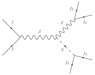
Figure 1: A Feynman diagram of the Higgs-strahlung.

Due to the energy-momentum conservation in process (1),

$$a_{1}=s,\qquad a_{2}\in(4m_{f_{Z}}^{2},(\sqrt{a_{1}}-\sqrt{a_{X}})^{2}),\qquad a_{X}\in(4m_{f_{X}}^{2},(\sqrt{a_{1}}-2m_{f_{Z}})^{2}),$$ (2)

where $a_{1}$, $a_{2}$, and $a_{X}$ are the squared invariant masses of the $Z$ boson (called $Z_{1}$) produced by the fermion-antifermion pair $f\bar{f}$, of the $Z$ boson (called $Z_{2}$) produced together with the boson $X$, and of the boson $X$ itself, respectively, $s$ is the squared invariant energy of $f\bar{f}$, $m_{f_{Z}}$ and $m_{f_{X}}$ are the masses of the fermions $f_{Z}$ and $f_{X}$ respectively.

The amplitude $A(\lambda_{1},\lambda_{2})$ of the transition $Z\to ZX$ is analogous to the $HVV$ amplitude in Ref. the_hZZ_couplings_CMS (see Eq. (1) there) and to the $XZZ$ amplitude in Ref. the_XZZ_amplitude_1 (Eq. (7)) and in the_XZZ_amplitude_2 (Eq. (3)):

$$A(\lambda_{1},\lambda_{2})= 2\sqrt{\sqrt{2}G_{F}}m_{Z}^{2}\Biggl{(}\left(g_{1}(a_{1},a_{2})-\frac{a_{1}+a_{2}-a_{X}}{m_{Z}^{2}}g_{2}(a_{1},a_{2})\right)(e_{1}\cdot e_{2}^{*})$$

$$+2\frac{g_{2}(a_{1},a_{2})}{m_{Z}^{2}}(e_{1}\cdot q_{2})(e_{2}^{*}\cdot q_{1})+2\frac{g_{3}(a_{1},a_{2})}{m_{Z}^{2}}\varepsilon_{\mu\nu\rho\sigma}q_{1}^{\mu}q_{2}^{\nu}e_{1}^{\rho}(e_{2}^{\sigma})^{*}\Biggr{)},$$ (3)

where $\lambda_{j}$, $e_{j}$, and $q_{j}$ are the helicity, polarization 4-vector, and 4-momentum of the boson $Z_{j}$ respectively ($j=1,2$), $G_{F}$ is the Fermi constant, $m_{Z}$ is the pole mass of the $Z$ boson, $g_{1}(a_{1},a_{2})$, $g_{2}(a_{1},a_{2})$, and $g_{3}(a_{1},a_{2})$ are some complex-valued functions on $a_{1}$ and $a_{2}$ — we call these functions $XZZ$ couplings, $\varepsilon_{\mu\nu\rho\sigma}$ is the Levi-Civita symbol ($\varepsilon_{0123}=1$). In Ref. the_hZZ_couplings_CMS the $XZZ$ couplings are denoted as $a_{1}$, $a_{2}$, and $a_{3}$ — we denote them as $g_{1}$, $g_{2}$, and $g_{3}$ respectively to avoid confusion.

At the tree level, the $XZZ$ couplings are connected with the CP parity of the boson $X$, as shown in Table 1. In the SM $g_{1}=1$ and $g_{2}=g_{3}=0$.

Table 1: The $CP$ parity of the particle $X$ for various values of $g_{1}$, $g_{2}$, and $g_{3}$.

$g_{1}$	$g_{2}$	$g_{3}$	$CP_{X}$
any	any	0	1
0	0	$\neq$ 0	$-1$
$\neq$ 0	any	$\neq$ 0	indefinite
any	$\neq 0$	$\neq 0$

In the $Z_{1}$ rest frame, or the center-of-mass frame of process (1), the polarization vectors read:

$$e_{1}^{\mu}|_{\lambda_{1}=0}=(0,0,0,1),\qquad e_{1}^{\mu}|_{\lambda_{1}=\pm 1}=(0,\mp\frac{1}{\sqrt{2}},\frac{i}{\sqrt{2}},0),$$ (4)

$$e_{2}^{\mu}|_{\lambda_{2}=0}=(\frac{|\mathbf{q_{2}}|}{\sqrt{a_{2}}},0,0,-\frac{\sqrt{|\mathbf{q_{2}}|^{2}+a_{2}}}{\sqrt{a_{2}}}),\qquad e_{2}^{\mu}|_{\lambda_{2}=\pm 1}=(0,\pm\frac{1}{\sqrt{2}},\frac{i}{\sqrt{2}},0).$$ (5)

Using Eqs. (II), (4) and (5), we derive that

$$A(-1,1)=-g_{1}-\frac{a_{X}-a_{1}-a_{2}}{m_{Z}^{2}}g_{2}+2i\frac{\sqrt{a_{1}}|\mathbf{q_{2}}|}{m_{Z}^{2}}g_{3},$$

$$A(1,-1)=-g_{1}-\frac{a_{X}-a_{1}-a_{2}}{m_{Z}^{2}}g_{2}-2i\frac{\sqrt{a_{1}}|\mathbf{q_{2}}|}{m_{Z}^{2}}g_{3},$$

$$A(0,0)=(g_{1}+\frac{a_{X}-a_{1}-a_{2}}{m_{Z}^{2}}g_{2})\frac{\sqrt{|\mathbf{q_{2}}|^{2}+a_{2}}}{\sqrt{a_{2}}}+2\frac{\sqrt{a_{1}}|\mathbf{q_{2}}|^{2}}{m_{Z}^{2}\sqrt{a_{2}}}g_{2},$$

$$A(\lambda_{1},\lambda_{2})=0\quad{\rm for}\quad\lambda_{1}\neq-\lambda_{2}.$$ (6)

The amplitude of the decay $X\to f_{X}\bar{f}_{X}$ is the_amplitude_of_the_X_to_f_antif_transition

$$A_{X\to f_{X}\bar{f}_{X}}(\lambda_{f_{X}},\lambda_{\bar{f}_{X}})=-\sqrt{\sqrt{2}G_{F}}m_{f_{X}}\bar{u}_{f_{X}}(\rho_{1}+\rho_{2}\gamma^{5})v_{\bar{f}_{X}},$$ (7)

where $u$ and $v$ are the Dirac spinors, $\lambda_{f_{X}}$ ($\lambda_{\bar{f}_{X}}$) is the helicity of the fermion (antifermion), $\rho_{1}$ and $\rho_{2}$ are some complex numbers which we call the $Xff$ couplings. In the SM $\rho_{1}=1$ and $\rho_{2}=0$.

Calculation of $A_{X\to f_{X}\bar{f}_{X}}(\lambda_{f_{X}},\lambda_{\bar{f}_{X}})$ in the $X$ rest frame yields

$$A_{X\to f_{X}\bar{f}_{X}}(-\frac{1}{2},-\frac{1}{2})=\sqrt{\sqrt{2}G_{F}}m_{f_{X}}(\rho_{1}+\rho_{2})\sqrt{a_{X}},$$

$$A_{X\to f_{X}\bar{f}_{X}}(\frac{1}{2},\frac{1}{2})=\sqrt{\sqrt{2}G_{F}}m_{f_{X}}(\rho_{1}-\rho_{2})\sqrt{a_{X}},$$

$$A_{X\to f_{X}\bar{f}_{X}}(-\frac{1}{2},\frac{1}{2})=A_{X\to f_{X}\bar{f}_{X}}(\frac{1}{2},-\frac{1}{2})=0.$$ (8)

Using the helicity formalism and neglecting $m_{f}$, $m_{f_{Z}}$, and $m_{f_{X}}$ everywhere save the $m_{f_{X}}$ factor in Eq. (II), we derive the fully differential cross section of process (1):

$$\frac{d^{7}\sigma}{da_{2}da_{X}d\theta_{Z}d\theta_{f_{Z}}d\phi d\theta_{f_{X}}d\phi_{f_{X}}}=\frac{G_{F}^{4}m_{Z}^{8}m_{f_{X}}^{2}}{(4\pi)^{7}}\cdot\frac{a_{2}a_{X}\lambda^{1/2}(s,a_{2},a_{X})}{sD(s)D(a_{2})D_{X}(a_{X})}(a_{f}^{2}+v_{f}^{2})(a_{f_{Z}}^{2}+v_{f_{Z}}^{2})$$

$$\times(|\rho_{1}|^{2}+|\rho_{2}|^{2})\sin\theta_{Z}\sin\theta_{f_{Z}}\sin\theta_{f_{X}}\Biggl{[}(|A_{\parallel}|^{2}+|A_{\perp}|^{2})\Bigl{(}P_{1}(1+\cos^{2}\theta_{Z})(1+\cos^{2}\theta_{f_{Z}})$$

$$+4P_{2}A_{f_{Z}}\cos\theta_{Z}\cos\theta_{f_{Z}}\Bigr{)}+{\rm Re}(A_{\parallel}^{*}A_{\perp})\cdot 4\Bigl{(}P_{1}A_{f_{Z}}\cos\theta_{f_{Z}}(1+\cos^{2}\theta_{Z})$$

$$+P_{2}\cos\theta_{Z}(1+\cos^{2}\theta_{f_{Z}})\Bigr{)}+|A_{0}|^{2}\cdot 4P_{1}\sin^{2}\theta_{Z}\sin^{2}\theta_{f_{Z}}-4\sqrt{2}\sin\theta_{Z}\sin\theta_{f_{Z}}$$

$$\times\Bigl{(}({\rm Re}(A_{0}^{*}A_{\parallel})\cos\phi+{\rm Im}(A_{0}^{*}A_{\perp})\sin\phi)(P_{2}A_{f_{Z}}+P_{1}\cos\theta_{Z}\cos\theta_{f_{Z}})$$

$$+({\rm Im}(A_{0}^{*}A_{\parallel})\sin\phi+{\rm Re}(A_{0}^{*}A_{\perp})\cos\phi)(P_{1}A_{f_{Z}}\cos\theta_{Z}+P_{2}\cos\theta_{f_{Z}})\Bigr{)}+P_{1}\sin^{2}\theta_{Z}\sin^{2}\theta_{f_{Z}}$$

$$\times\Bigl{(}(|A_{\parallel}|^{2}-|A_{\perp}|^{2})\cos 2\phi+{\rm Im}(A_{\parallel}^{*}A_{\perp})\cdot 2\sin 2\phi\Bigr{)}\Biggr{]},$$ (9)

where (see Fig. 2)

• $\theta_{Z}$ is the angle between the momentum $\mathbf{p}_{f}$ of the fermion $f$ in the $f\bar{f}$ rest frame and the momentum $\mathbf{q}_{2}$ of the $Z$ boson $Z_{2}$ in the same frame;

• $\theta_{f_{Z}}$ is the angle between $\mathbf{q}_{2}$ and the $f_{Z}$ momentum $\mathbf{p}_{f_{Z}}$ in the $Z_{2}$ rest frame;

• $\phi$ is the azimuthal angle between the plane spanned by the vectors $\mathbf{p}_{f}$ and $\mathbf{q}_{2}$ and the plane spanned by $\mathbf{q}_{2}$ and $\mathbf{p}_{f_{Z}}$;

• $\theta_{f_{X}}$ is the angle between the $X$ momentum in the $f\bar{f}$ rest frame and the $f_{X}$ momentum in the $X$ rest frame;

• $\phi_{f_{X}}$ is the azimuthal angle of the fermion $f_{X}$;

• $\lambda(x,y,z)\equiv x^{2}+y^{2}+z^{2}-2(xy+xz+yz)$;

• $D(x)\equiv(x-m_{Z}^{2})^{2}+(m_{Z}\Gamma_{Z})^{2}$,  $D_{X}(x)\equiv(x-m_{X}^{2})^{2}+(m_{X}\Gamma_{X})^{2}$;

• $\Gamma_{Z}$ ($\Gamma_{X}$) is the total width of the $Z$ ($X$) boson;

• $m_{X}$ is the pole mass of the $X$ boson;

• $a_{f}$ is the projection of the weak isospin of a fermion $f$, $v_{f}\equiv a_{f}-2\frac{q_{f}}{e}\sin^{2}\theta_{W}$, $q_{f}$ is the electric charge of the fermion $f$, $e$ is the electric charge of the positron, $\theta_{W}$ is the weak mixing angle, $A_{f}\equiv\frac{2a_{f}v_{f}}{a_{f}^{2}+v_{f}^{2}}$;

• $A_{0}\equiv\frac{s+a_{2}-a_{X}}{2\sqrt{sa_{2}}}g_{1}-\frac{2\sqrt{sa_{2}}}{m_{Z}^{2}}g_{2}$, $A_{\parallel}\equiv-\frac{A(-1,1)+A(1,-1)}{\sqrt{2}}=\sqrt{2}\left(g_{1}-\frac{s+a_{2}-a_{X}}{m_{Z}^{2}}g_{2}\right)$, $A_{\perp}\equiv-\frac{A(-1,1)-A(1,-1)}{\sqrt{2}}=i\sqrt{2}\frac{\lambda^{1/2}(s,a_{2},a_{X})}{m_{Z}^{2}}g_{3}$;

• $P_{1}\equiv 1-P_{f}P_{\bar{f}}-(P_{f}-P_{\bar{f}})A_{f}$,   $P_{2}\equiv(1-P_{f}P_{\bar{f}})A_{f}-P_{f}+P_{\bar{f}}$, where $P_{f}$ ($P_{\bar{f}}$) is the fermion (antifermion) beam longitudinal polarization.

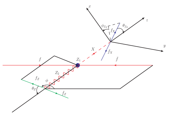
Figure 2: Kinematics of process (1). The momenta of $f$, $\bar{f}$, $Z_{1}$, $X$, and $Z_{2}$ are shown in the $f\bar{f}$ rest frame, the momenta of $f_{Z}$ and $\bar{f}_{Z}$ are displayed in the $Z_{2}$ rest frame, the momenta of $f_{X}$ and $\bar{f}_{X}$ are described in the $X$ rest frame. The $z$ axis is co-directional with the $X$ momentum while the $x$ and $y$ axes are arbitrary axes forming a right-handed system with the $z$ axis.

According to Eq. (II), all the possible directions of the $f_{X}$ momentum in the $X$ rest frame are equiprobable. Having measured an observable describing Higgs-strahlung (1), one will be able to use Eq. (II) and to put some constraints on the functions $A_{0}$, $A_{\parallel}$, and $A_{\perp}$, thus getting possible intervals for the $XZZ$ couplings $g_{1}$, $g_{2}$, and $g_{3}$.

The differential cross section of the process $e^{-}e^{+}\to f\bar{f}h$ is obtained in Ref. the_Higgs_strahlung_fully_differential_cross_section_without_consideration_of_the_Higgs_boson_decay . However, considering process (1), we take into account that the boson $X$ decays, which happens in reality. Moreover, integration of Eq. (II) yields more precise total and differential cross sections and observables than those which can be derived by integration of the fully differential cross section of $e^{-}e^{+}\to f\bar{f}h$. The reason is that we can integrate (II) with respect to $a_{X}$ without the narrow-width approximation and with any desired accuracy.

Integration of Eq. (II) with the narrow-width approximation for both $Z$ and $X$ boson yields the total cross section of the Higgs-strahlung:

$$\sigma= \frac{G_{F}^{4}m_{Z}^{9}m_{X}m_{f_{X}}^{2}}{288\pi^{3}\Gamma_{Z}\Gamma_{X}}\cdot\frac{\lambda^{1/2}(s,m_{Z}^{2},m_{X}^{2})}{sD(s)}(a_{f}^{2}+v_{f}^{2})(a_{f_{Z}}^{2}+v_{f_{Z}}^{2})(|\rho_{1}|^{2}+|\rho_{2}|^{2})P_{1}$$

$$\times\sum_{p=0,\parallel,\perp}|A_{p}|^{2}\Bigl{|}_{a_{2}=m_{Z}^{2},\,a_{X}=m_{X}^{2}}.$$ (10)

Since $\sigma\sim P_{1}$, the total cross section has its largest value at $P_{f}=-1$ and $P_{\bar{f}}=1$ if $A_{f}>0$.

III Optimal observables

In this section we demonstrate how differential cross section (II) can be used to determine the couplings $g_{1},g_{2},g_{3}$ after kinematic information on a number of events (1) is obtained. For this purpose, the method of Refs. optimal_observables_—_a_one-dimensional_case ; optimal_observables_—_a_multidimensional_case is applied. According to optimal_observables_—_a_one-dimensional_case ; optimal_observables_—_a_multidimensional_case , if the fully differential cross section of a process can be presented in the form

$$\frac{d\sigma}{dk}=S_{0}(k)+\sum\limits_{i=1}^{n}h_{i}S_{i}(k),$$ (11)

where $k$ denotes all the kinematic variables of this process, $S_{0}(k),S_{1}(k),\ldots,S_{n}(k)$ are functions of $k$,  $h_{i}$ ($i=1,\ldots,n$) are real-valued small (i.e. $h_{i}\to 0$) dimensionless parameters independent of $k$, then measurement of an observable

$$O_{i}\equiv\frac{1}{\sigma}\int dk\frac{d\sigma}{dk}\cdot\frac{S_{i}(k)}{S_{0}(k)}$$ (12)

yields the tightest constraint on the parameter $h_{i}$. “The tightest constraint on a parameter” means an experimental value of the parameter with the least standard deviation which is possible for measured data for the studied process. In (12) $\sigma$ is the total cross section of the process:

$$\sigma\equiv\int dk\frac{d\sigma}{dk}.$$ (13)

The integration in Eqs. (12) and (13) is performed over all the possible values of the variables $k$. In Ref. optimal_observables_—_a_multidimensional_case observables (12) are called optimal.

In our case, differential cross section (II) can be rewritten as

$$\frac{d\sigma}{dk}= (|\rho_{1}|^{2}+|\rho_{2}|^{2})\Bigr{[}f_{SM}(k)+(|g_{1}|^{2}-1)f_{1}(k)+|g_{2}|^{2}f_{2}(k)+|g_{3}|^{2}f_{3}(k)$$

$$+{\rm Re}(g_{1}^{*}g_{2})f_{4}(k)+{\rm Re}(g_{1}^{*}g_{3})f_{5}(k)+{\rm Re}(g_{2}^{*}g_{3})f_{6}(k)$$

$$+{\rm Im}(g_{1}^{*}g_{2})f_{7}(k)+{\rm Im}(g_{1}^{*}g_{3})f_{8}(k)+{\rm Im}(g_{2}^{*}g_{3})f_{9}(k)\Bigl{]},$$ (14)

where $dk\equiv da_{2}da_{X}d\theta_{Z}d\theta_{f_{Z}}d\phi d\theta_{f_{X}}d\phi_{f_{X}}$ and $f_{SM}(k),f_{1}(k)=f_{SM}(k),f_{2}(k),f_{3}(k),\ldots,f_{9}(k)$ are some particular functions of the invariant masses squared $a_{2}$, $a_{X}$, of the angular variables $\theta_{Z}$, $\theta_{f_{Z}}$, $\phi$, $\theta_{f_{X}}$, of the polarizations $P_{f}$, $P_{\bar{f}}$, and of the squared invariant energy $s$.

In the SM

$$\frac{d\sigma}{dk}=(|\rho_{1}|^{2}+|\rho_{2}|^{2})f_{SM}(k).$$ (15)

We suppose that the couplings $g_{1}$, $g_{2}$, and $g_{3}$ in (II) are close to their SM values and do not depend on $a_{1}$ or $a_{2}$, i.e., $g_{1}(a_{1},a_{2})\approx 1$, $g_{2}(a_{1},a_{2})\approx 0$, $g_{3}(a_{1},a_{2})\approx 0$. Then Eq. (III) has the form of Eq. (11) with $n=9$ and

$$S_{0}(k)=S_{1}(k)=(|\rho_{1}|^{2}+|\rho_{2}|^{2})f_{SM}(k),$$

$$S_{2}(k)=(|\rho_{1}|^{2}+|\rho_{2}|^{2})\,f_{2}(k),$$

$$\ldots$$

$$S_{9}(k)=(|\rho_{1}|^{2}+|\rho_{2}|^{2})\,f_{9}(k),$$

$$h_{1}=|g_{1}|^{2}-1,\;h_{2}=|g_{2}|^{2},\;h_{3}=|g_{3}|^{2},$$

$$h_{4}={\rm Re}(g_{1}^{*}g_{2}),\;\ldots,\;h_{9}={\rm Im}(g_{2}^{*}g_{3}).$$ (16)

Therefore, the observable $O_{1}$ for the Higgs-strahlung is

$$O_{1}\equiv\frac{1}{\sigma}\int dk\frac{d\sigma}{dk}=1.$$ (17)

Thus this observable provides no information on the quantity $|g_{1}|^{2}-1$, i.e. no constraint on $|g_{1}|$. If we measure the fully differential distribution $\frac{1}{\sigma}\frac{d\sigma}{dk}$ of the Higgs-strahlung, we will gain no constraint on $|g_{1}|$ as well. The reason is that according to Eq. (III), the dependence of $\frac{1}{\sigma}\frac{d\sigma}{dk}$ on the couplings $g_{1}$, $g_{2}$, and $g_{3}$ reduces only to a dependence on the fractions $\frac{g_{2}}{g_{1}}$ and $\frac{g_{3}}{g_{1}}$. Thus, measurement of the fully differential distribution yields constraints only on the latter fractions. To constrain $|g_{1}|$, one can measure $\sigma$.

We calculate numerically the observables

$$O_{i}\equiv\frac{1}{\sigma}\int dk\frac{d\sigma}{dk}\frac{f_{i}(k)}{f_{SM}(k)},\qquad i=2,3,\ldots,9$$ (18)

for process (1) with $f=e$, using the values listed in Table 2. In this table we show the $\sqrt{s}$, $P_{e^{-}}$, and $P_{e^{+}}$ values planned for the first stage of the ILC (see the_Linear_Collider_Collaboration_strategy_on_measuring_the_Higgs_boson_properties ).

Table 2: The parameters used to calculate optimal observables (18) for the Higgs-strahlung. These parameters are taken from Refs. the_Linear_Collider_Collaboration_strategy_on_measuring_the_Higgs_boson_properties ; the_2016_review_of_particle_physics_by_the_Particle_Data_Group . For $\Gamma_{h}$ we use its SM value.

$P_{e^{-}}=-0.8$,  $P_{e^{+}}=0.3$,  $\sqrt{s}=250$ GeV
$A_{e}=0.1515$
$m_{h}=125.09$ GeV,  $\Gamma_{h}=4.15$ MeV
$m_{Z}=91.1876$ GeV,  $\Gamma_{Z}=2.4952$ GeV

Observables (18) calculated for process (1) with $f=f_{Z}=e$ and $f_{X}=e,\mu,\tau,u,d,s,c,b$ are

$$O_{2}= \,G^{-1}\Bigl{(}{34.1+1281.8\,|\frac{g_{2}}{g_{1}}|^{2}+311.2\,|\frac{g_{3}}{g_{1}}|^{2}-395.4\,{\rm Re}(\frac{g_{2}}{g_{1}})}\Bigr{)},$$

$$O_{3}= \,G^{-1}\Bigl{(}{8.0+311.2\,|\frac{g_{2}}{g_{1}}|^{2}+82.7\,|\frac{g_{3}}{g_{1}}|^{2}-94.0\,{\rm Re}(\frac{g_{2}}{g_{1}})}\Bigr{)},$$

$$O_{4}= \,G^{-1}\Bigl{(}{-11.5-395.4\,|\frac{g_{2}}{g_{1}}|^{2}-94.0|\frac{g_{3}}{g_{1}}|^{2}+132.9\,{\rm Re}(\frac{g_{2}}{g_{1}})}\Bigr{)},$$

$$O_{5}= \,G^{-1}\Bigl{(}{1.1\,{\rm Re}(\frac{g_{3}}{g_{1}})-6.6\,{\rm Re}((\frac{g_{2}}{g_{1}})^{*}\frac{g_{3}}{g_{1}})}\Bigr{)},$$

$$O_{6}= \,G^{-1}\Bigl{(}{-6.6\,{\rm Re}(\frac{g_{3}}{g_{1}})+40.1\,{\rm Re}((\frac{g_{2}}{g_{1}})^{*}\frac{g_{3}}{g_{1}})}\Bigr{)},$$

$$O_{7}= \,G^{-1}\cdot{0.24\,{\rm Im}(\frac{g_{2}}{g_{1}})},$$

$$O_{8}= \,G^{-1}\Bigl{(}{13.6\,{\rm Im}(\frac{g_{3}}{g_{1}})-88.7\,{\rm Im}((\frac{g_{2}}{g_{1}})^{*}\frac{g_{3}}{g_{1}})}\Bigr{)},$$

$$O_{9}= \,G^{-1}\Bigl{(}{-88.7\,{\rm Im}(\frac{g_{3}}{g_{1}})+583.4\,{\rm Im}((\frac{g_{2}}{g_{1}})^{*}\frac{g_{3}}{g_{1}})}\Bigr{)},$$ (19)

where

$$G\equiv 1+34.1\left|\frac{g_{2}}{g_{1}}\right|^{2}+8.0\left|\frac{g_{3}}{g_{1}}\right|^{2}-11.5\,{\rm Re}\left(\frac{g_{2}}{g_{1}}\right).$$ (20)

Observables (III) depend only on the ratios $\frac{g_{2}}{g_{1}}$ and $\frac{g_{3}}{g_{1}}$. Thus their measurement gives constraints only on the real quantities ${\rm Re}(\frac{g_{2}}{g_{1}})$, ${\rm Im}(\frac{g_{2}}{g_{1}})$, ${\rm Re}(\frac{g_{3}}{g_{1}})$, and ${\rm Im}(\frac{g_{3}}{g_{1}})$.

If the couplings $g_{1}$, $g_{2}$, and $g_{3}$ are real, the Lagrangian describing the interaction of the Higgs boson with two $Z$ bosons is Hermitian. Considering only real values of $\frac{g_{2}}{g_{1}}$ and $\frac{g_{3}}{g_{1}}$, we present plots of the observables $O_{2},\ldots,O_{6}$ in Fig. 3. The observables $O_{7}$, $O_{8}$, and $O_{9}$ are all zero if $\frac{g_{2}}{g_{1}}$ and $\frac{g_{3}}{g_{1}}$ are real (see Eqs. (III)).

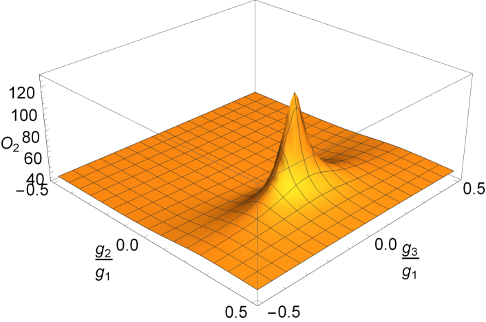
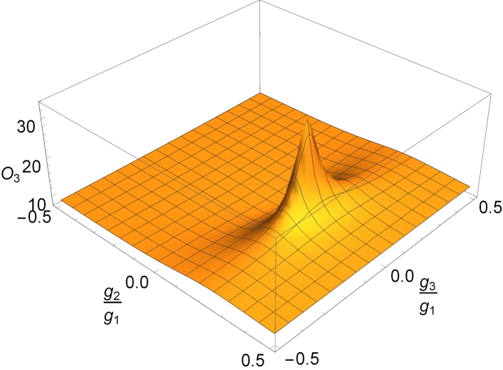
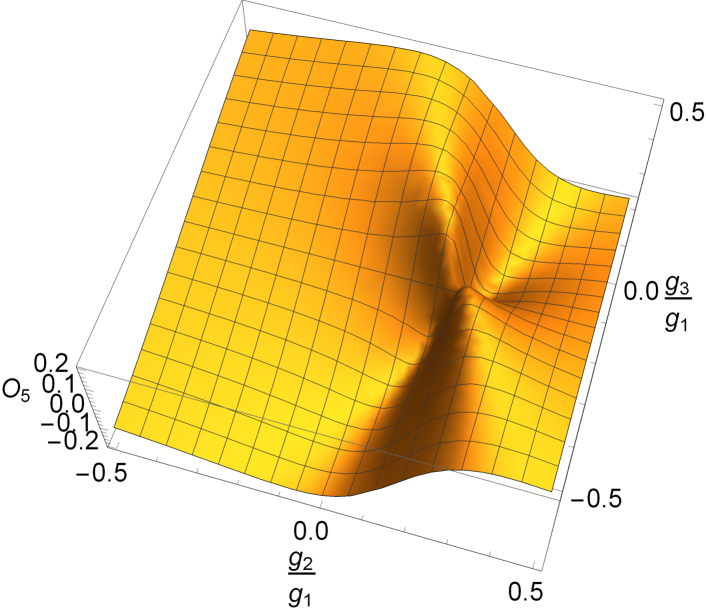
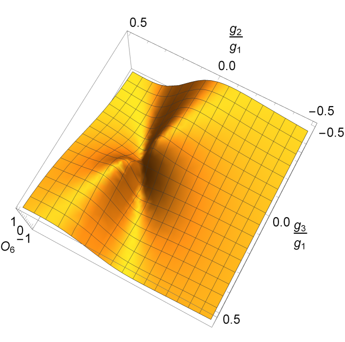
Figure 3: Plots of the observables $O_{2},\ldots,O_{6}$ for $\frac{g_{2}}{g_{1}},\frac{g_{3}}{g_{1}}\in[-0.5,0.5]$.

The observables $O_{2}$, $O_{3}$, and $O_{4}$ are approximately proportional to each other. Moreover, we have analytically investigated the critical points of $O_{2},\ldots,O_{6}$. Our calculation shows that each of $O_{2}$, $O_{3}$, and $O_{4}$ has a local maximum at $\frac{g_{2}}{g_{1}}\approx 0.17$ and $\frac{g_{3}}{g_{1}}=0$. Both $O_{5}$ and $O_{6}$ have a saddle point at the same point $\frac{g_{2}}{g_{1}}\approx 0.17$, $\frac{g_{3}}{g_{1}}=0$. The closer the values of $O_{2},\ldots,O_{6}$ are to their values at the maximum or saddle points, the faster these observables change and the tighter constraints on $\frac{g_{2}}{g_{1}}$ and $\frac{g_{3}}{g_{1}}$ these observables provide.

If one calculates observables (18) for process (1) with $f=e$, $f_{Z}=e,\mu$ and $f_{X}=e,\mu,\tau,u,d,s,c,b$, then in the approximation $A_{e}=A_{\mu}$ the result still will be Eqs. (III). If you want to take into account the difference between $A_{e}$ and $A_{\mu}$ ($A_{e}=0.1515$ and $A_{\mu}=0.142$ the_2016_review_of_particle_physics_by_the_Particle_Data_Group ), you can edit Supplemental Material a_Mathematica_notebook . Moreover, in an experiment events (1) cannot be measured with all the possible values of the kinematic variables $k$. To account for that, one can change the limits of integration for observables (18) in a_Mathematica_notebook .

IV Conclusions

We have derived the fully differential cross section of the Higgs-strahlung process $f\bar{f}\to Z\to ZX\to f_{Z}\bar{f}_{Z}f_{X}\bar{f}_{X}$, where $f$, $f_{Z}$, and $f_{X}$ are arbitrary fermions, $X$ is a particle with zero spin and arbitrary $ZZ$ and $ff$ couplings. This process with $f=e$, $X=h$, $f_{Z}=e,\mu,u,d,s,c,b$, and $f_{h}=\tau,b$ is going to be measured at the ILC.

We have defined observables measurement of which gives the tightest constraints on the Higgs boson couplings $g_{1}$, $g_{2}$, $g_{3}$ to $Z$ bosons. These observables are called optimal. Their explicit dependences on $g_{i}$ are presented. The sensitivity of the observables to the couplings is analyzed. Therefore, after the optimal observables are measured at the ILC, one can constrain the Higgs boson couplings $g_{i}$. Using a_Mathematica_notebook , one can account for experimental constraints on the kinematic variables or derive explicit expressions of optimal observables for other similar processes.

References

(1)
G. Aad et al. (ATLAS Collaboration),
Phys. Lett. B 716, 1 (2012).
(2)
S. Chatrchyan et al. (CMS Collaboration),
Phys. Lett. B 716, 30 (2012).
(3)
P. W. Higgs,
Phys. Rev. Lett. 13, 508 (1964).
(4)
A. M. Sirunyan et al. (CMS Collaboration),
Phys. Lett. B 775, 1 (2017).
(5)
M. Aaboud et al. (ATLAS Collaboration),
arXiv:1712.02304 [hep-ex].
(6)
G. Aad et al. (ATLAS and CMS Collaborations),
JHEP 1608 (2016) 045.
(7)
D. M. Asner et al.,
arXiv:1310.0763 [hep-ph].
(8)
I. Anderson et al.,
Phys. Rev. D 89, no. 3, 035007 (2014).
(9)
M. Hashemi,
arXiv:1805.10513 [hep-ph].
(10)
P. Drechsel, G. Moortgat-Pick, and G. Weiglein,
arXiv:1801.09662 [hep-ph].
(11)
D. Barducci and A. J. Helmboldt,
JHEP 1712, 105 (2017).
(12)
T. Kamon, P. Ko, and J. Li,
Eur. Phys. J. C 77, no. 9, 652 (2017).
(13)
A. Angelescu, G. Moreau, and F. Richard,
Phys. Rev. D 96, no. 1, 015019 (2017).
(14)
G. L. Liu, F. Wang, K. Xie and X. F. Guo,
Phys. Rev. D 96, no. 3, 035005 (2017).
(15)
M. Frank, K. Huitu, U. Maitra, and M. Patra,
Phys. Rev. D 94, no. 5, 055016 (2016).
(16)
I. Chakraborty, A. Datta and A. Kundu,
J. Phys. G 43, no. 12, 125001 (2016).
(17)
S. Banerjee, B. Bhattacherjee, M. Mitra and M. Spannowsky,
JHEP 1607, 059 (2016).
(18)
J. P. Ma and B. H. J. McKellar,
Phys. Rev. D 52, 22 (1995).
(19)
T. Han and J. Jiang,
Phys. Rev. D 63, 096007 (2001).
(20)
D. Chang, W. Y. Keung and I. Phillips,
Phys. Rev. D 48, 3225 (1993).
(21)
K. Rao and S. D. Rindani,
Phys. Lett. B 642, 85 (2006).
(22)
I. Anderson et al.,
Phys. Rev. D 89, no. 3, 035007 (2014).
(23)
D. Atwood and A. Soni,
Phys. Rev. D 45, 2405 (1992).
(24)
M. Diehl, O. Nachtmann, and F. Nagel,
Eur. Phys. J. C 27, 375 (2003).
(25)
T. V. Zagoskin and A. Y. Korchin,
Int. J. Mod. Phys. A 32, no. 27, 1750166 (2017).
(26)
T. V. Zagoskin and A. Y. Korchin,
J. Exp. Theor. Phys. 122, no. 4, 663 (2016).
(27)
Y. Gao, A. V. Gritsan, Z. Guo, K. Melnikov, M. Schulze, and N. V. Tran,
Phys. Rev. D 81, 075022 (2010).
(28)
K. Hagiwara and M. L. Stong,
Z. Phys. C 62, 99 (1994)
(29)
C. Patrignani et al. (Particle Data Group),
Chin. Phys. C 40, 100001 (2016) and 2017 update.
(30)
A Mathematica notebook where the optimal observables for the Higgs-strahlung are worked out is available from the authors upon request.