Joint Deformable Registration of Large EM Image Volumes: A Matrix Solver Approach

Abstract

Large electron microscopy image datasets for connectomics are typically composed of thousands to millions of partially overlapping two-dimensional images (tiles), which must be registered into a coherent volume prior to further analysis. A common registration strategy is to find matching features between neighboring and overlapping image pairs, followed by a numerical estimation of optimal image deformation using a so-called solver program.

Existing solvers are inadequate for large data volumes, and inefficient for small-scale image registration.

In this work, an efficient and accurate matrix-based solver method is presented. A linear system is constructed that combines minimization of feature-pair square distances with explicit constraints in a regularization term. In absence of reliable priors for regularization, we show how to construct a rigid-model approximation to use as prior. The linear system is solved using available computer programs, whose performance on typical registration tasks we briefly compare, and to which future scale-up is delegated. Our method is applied to the joint alignment of 2.67 million images, with more than 200 million point-pairs and has been used for successfully aligning the first full adult fruit fly brain.

1 Introduction

Electron microscopy (EM) images contain anatomical information relevant for detailed reconstruction of neuronal circuits. Modern EM acquisition systems produce increasingly large sample volumes, with millions of images (Zheng et al., 2017). Due to the limited field-of-view of current imaging hardware, and the desire to image large volumes, partially overlapping images (tiles) are acquired, to be registered into a seamless three-dimensional volume in a post-acquisition processing step. Analysis is performed on such fully registered image volumes (Takemura et al., 2015; ya Takemura et al., 2013; Bock et al., 2011; Saalfeld et al., 2010, 2012; Scheffer et al., 2013; Cardona et al., 2012).

A major challenge for EM volume registration is the large dataset size. For example, to image a whole fruit-fly brain (approximately 500 µm in its largest dimension) at voxel dimensions of 4×4×40 nm³ with serial section transmission EM (ssTEM), with 10% overlap of adjacent tiles, approximately 21 million images ($\approx$380 tera voxels) are generated (Zheng et al., 2017). There is a need for robust, efficient and scalable methods for registering such volumes.

This manuscript addresses three stages of EM volume registration:

Montage registration

The process by which partially overlapping images within the same section are registered to form a seamless mosaic (Figure 1b),

Rough alignment

Scaled-down snapshots of whole montages produced by the previous step are roughly registered to each other across $z$, and finally,

Fine alignment

In which point-matches obtained from step 1, together with point-matches across sections are used to jointly register the whole volume.

Each of the above steps is itself a two-step process. First: Matching point-pairs are found between pairs of images identified as potential neighbors (Figure 1a and b (left panel)), based on matching image features (Lowe, 2004; Saalfeld et al., 2010, 2012). Second: Using that set of point matches, and after deciding on a transformation model, image transformation parameters are estimated by a solver algorithm. The algorithm minimizes the sum of squared distances between all point matches (Figure 1). Deforming tiles according to these estimated transformations ideally results in a seamless registration of the whole volume (Figure 1e).

Available solver algorithms for EM use point-match information local to each tile to find a local solution, move a step towards that solution, iterate similarly over all tiles and repeat the process until a convergence criterion is satisfied. The solver by Karsh (2016), although scalable to large problem sizes, is based on the local iterative scheme described above, regularizes against stage coordinates which are often unreliable, and is not guaranteed to converge to a global optimum. The strategy by Saalfeld et al. (2010, 2012) is limited to smaller volumes than described in this work. Restriction to iterative techniques necessitates additional solver parameterization (maximum step size, number of iterations and other empirical termination criteria) and, at the least-squares level, limits accuracy. Other techniques, for example that by Tasdizen et al. (2010), compose pairwise transformations sequentially and are therefore prone to additive error.

Main contributions of this work:

(a) We provide a formulation of model-based registration in linear algebra terms, to perform joint optimization of all images with explicit regularization. We thereby delegate both scalability and convergence of the solver to efficient established linear algebra computer programs that may or may not be iterative (and are generally more efficient even when iterative). For small to moderate problem sizes, our method thus uses reliable fast direct methods, which are parameter free at the least-squares level, and outperform all iterative approaches. For large problem sizes, known iterative techniques can be used. Moreover, nonlinear models, such as higher order polynomials, and arbitrary spatial dimensions are permitted in our matrix framework.

(b) We show how, in the absence of reliable starting guesses for tile transformations, a rigid model approximation can be estimated and used for explicit regularization. The presented method therefore assumes no prior knowledge of image orientation or relative scale, but can take full advantage of priors when provided.

In practice, tiles must be corrected for non-affine lens-distortion prior to montaging for which we used the method by Kaynig et al. (2010) followed by affine normalization. We further converted the final solution of the method described in this manuscript to a thin-plate spline (Bookstein, 1989) warp-field that we applied to the seamlessly stitched montages. This way, we retain the overall shape of the deformable registration approximated by an affine transformation for each tile while avoiding discontinuous seams between tiles in the montage.

2 Methods

2.1 The least-squares system

For a system of partially overlapping image tiles (number of tiles = $n_{\mathrm{tiles}}$), we assume that we are given a full set of point-matches between all neighboring tiles. We set up and solve a regularized (Tikhonov-like) least-squares system for finding the set of transformations $\mathbf{x}$ that optimally and jointly minimizes the square distances between all point-matches

$$\min_{\mathbf{x}}\lVert\mathbf{D}(\mathbf{A}\mathbf{x}-\mathbf{b})\rVert_{2}^{2}+\lambda\lVert\mathbf{B}\mathbf{x}-\mathbf{d}\rVert^{2}$$ (1)

The first term is the primary objective function. $\mathbf{A}$ is a large $m\times n$ matrix of point-pair correspondences. $\mathbf{x}$ is a column vector of transformation coefficients of length $n$, and $\mathbf{b}$ is a column vector of length $m$ ($\mathbf{A}$ and $\mathbf{b}$ are generally sparse). $n$ is a product of the total number of transformations ($n_{\mathrm{tiles}}$) and the number of coefficients ($n_{\mathrm{c}}$) for the type of transformation considered (e.g. $n_{\mathrm{c}}=6$ for two-dimensional affine). $m$ is the total number of point-pairs and $\mathbf{D}$ is the individual point-match confidence estimate. The second term is a regularization term in which $\mathbf{B}$ is a matrix with dimensions $n\times n$ and $d$ is a column vector of length $n$ with values that the solution $\mathbf{x}$ is expected to stay close to, i.e. it is an explicit regularization. $\mathbf{B}$ only has elements on the diagonal. $\lambda$ is a regularization parameter that controls the relative importance of fidelity of $\mathbf{x}$ to point-match data vs. adherence to values in $\mathbf{d}$. In practice, we generalize $\lambda$ to be a diagonal matrix which provides the ability to constrain individual parameters differently if desired.

2.2 Constructing $\mathbf{A}$: “No regularization” case

Let us first consider solving the first term of Equation 1 without regularization, i.e. without the second term in Equation 1. First, we construct $\mathbf{A}$ and $\mathbf{b}$. Matching point-pairs between overlapping tile pair $j$ are given by ${}^{j}_{i}{}p$ and ${}^{j}_{i}{}q$, with $j$ indicating the pair (e.g.: $j=(1,2)$ or $j=(5,8)$) and point index $i$. For reference see Figure 1. ${}^{j}_{i}{}p$ and ${}^{j}_{i}{}q$ are each 2-vectors (with columns ${}^{j}_{i}{}p_{x},^{j}_{i}{}p_{y}$ and ${}^{j}_{i}{}q_{x},^{j}_{i}{}q_{y}$). The length of ${}^{j}p$ and ${}^{j}q$ is $n_{j}$, and varies with the number of point-matches found between tiles in the pair $j$. $m$ is twice the sum of all $n_{j}$.

For example, we want to find two-dimensional transformations to register three overlapping image tiles jointly ($n_{\mathrm{tiles}}=3$), where each tile overlaps with the other two tiles

$$\tilde{\mathbf{A}}\mathbf{x}-\tilde{\mathbf{b}}=\begin{bmatrix}{}^{1,2}\mathrm{P}&-^{1,2}\mathrm{Q}&0\\ {}^{1,3}\mathrm{P}&0&-^{1,3}\mathrm{Q}\\ 0&{}^{2,3}\mathrm{P}&-^{2,3}\mathrm{Q}\end{bmatrix}\mathbf{x}-\begin{bmatrix}0\\ 0\\ 0\end{bmatrix}$$

where ${}^{j}\mathrm{P}$ and ${}^{j}\mathrm{Q}$ represent point-match matrix blocks for two connected tiles. ${}^{j}\mathrm{P}$ lists point coordinates in the first tile’s coordinate system and ${}^{j}\mathrm{Q}$ those in the second tile’s. The structure of these blocks depends on the transformation model chosen and reflects the basis functions considered.

For example, in case of an affine model, each point $(x,y)$ in tile coordinates is transformed to the common coordinate system $(u,v)$ such that

$$u =a_{1}x+a_{2}y+a_{0}$$

$$v =a_{4}x+a_{5}y+a_{3}$$

The parameters $a_{0},a_{1},\dots,a_{6}$ are the transformation parameters sought. The number of columns of $\mathbf{A}$ is $n=(n_{\mathrm{parameters}})\times(n_{\mathrm{tiles}})=18$, and the point-match blocks are given by

$${}^{j}\mathrm{P}=\begin{bmatrix}{}^{j}_{1}p_{x}&{}^{j}_{1}p_{y}&1&\dots&&\\ \vdots&\vdots&\vdots&\dots&&\\ {}^{j}_{n_{j}}p_{x}&{}^{j}_{n_{j}}p_{y}&1&\dots&&\\ &&&{}^{j}_{1}p_{x}&{}^{j}_{1}p_{y}&1\\ &&&\vdots&\vdots&\vdots\\ &&&{}^{j}_{n_{j}}p_{x}&{}^{j}_{n_{j}}p_{y}&1\end{bmatrix},~{}^{j}\mathrm{Q}=\begin{bmatrix}{}^{j}_{1}q_{x}&{}^{j}_{1}q_{y}&1&\dots&&\\ \vdots&\vdots&\vdots&\dots&&\\ {}^{j}_{n_{j}}q_{x}&{}^{j}_{n_{j}}q_{y}&1&\dots&&\\ &&&{}^{j}_{1}q_{x}&{}^{j}_{1}q_{y}&1\\ &&&\vdots&\vdots&\vdots\\ &&&{}^{j}_{n_{j}}q_{x}&{}^{j}_{n_{j}}q_{y}&1\end{bmatrix},~{}^{j}\mathrm{P}_{\mathrm{c}}=\begin{bmatrix}{}^{j}_{1}p_{x}\\ \vdots\\ {}^{j}_{n_{j}}p_{x}\\ {}^{j}_{1}p_{y}\\ \vdots\\ {}^{j}_{n_{j}}p_{y}\end{bmatrix},$$

in which $[^{j}_{n_{j}}p_{x},^{j}_{n_{j}}p_{y}]$ and $[^{j}_{n_{j}}q_{x},^{j}_{n_{j}}q_{y}]$ are two $x,y$ coordinates corresponding to images 1 and 2, in a coordinate system local to each image. It is instructive to keep the above non-reduced system in mind, even though it does not have a solution. To solve it, one image tile (in the above case we choose tile 1) must be fixed. This sets the frame of reference for all other transformations, such that

$$\mathbf{A}\mathbf{x}-\mathbf{b}=\begin{bmatrix}{}^{1,2}\mathrm{Q}&0\\ 0&-^{1,3}\mathrm{Q}\\ {}^{2,3}\mathrm{P}&-^{2,3}\mathrm{Q}\end{bmatrix}\mathbf{x}-\begin{bmatrix}{}^{1,2}\mathrm{P}_{\textrm{c}}\\ {}^{1,3}\mathrm{P}_{\textrm{c}}\\ 0\end{bmatrix}.$$ (2)

To fix a tile (done only for demonstration purposes here), the column range corresponding to its transformation parameters is eliminated. Vector $\mathbf{b}$ is modified as shown in Equation 2.

For small numbers of tiles, solving Equation 2 will yield the required transformations using standard linear solvers (see Figure 1 for an example with six tiles).

2.3 Regularization

The strategy of fixing one tile is not sufficient in the general case. With increasing numbers of tiles, and when tiles are further removed from the fixed reference tile, distortions are observed at the scale of the whole layer being stitched (Figures 2 and 2c left panel). To solve this problem, we include explicit constraints, by adding a regularization term (term 2 in Equation 1).

Stage-reported tile coordinates may be accurate enough to be used as an explicit constraint in special cases. However, in the general case, these numbers are not reliable. We now describe a strategy to obtain a rough guess ($\mathbf{d}$ in term 2 in Equation 1) to serve as regularizer. ${}^{j}_{i}{}p$ and ${}^{j}_{i}{}q$ are translated to their respective centers of mass, producing ${}^{j}_{i}\hat{p}$ and ${}^{j}_{i}\hat{q}$ . A two dimensional affine transformation can be constrained to a similarity deformation by considering, in addition to the point-match data ${}^{j}_{i}\hat{p}$ and ${}^{j}_{i}\hat{q}$, the point-match data subjected to an operator that transforms $(x,y)$ into $(-y,x)$ (Schaefer et al., 2006). We generalize this idea to the full set of point-matches among all tiles. The system is thereby implicitly similarity-deformation-constrained by the data; both original and artificially generated. To accomplish this, we write an equation similar to Equation 2 for the joint system

$$\mathbf{D}\mathbf{m}-\mathbf{f}=\begin{bmatrix}-^{1,2}\hat{\mathrm{Q}}&0\\ 0&-^{1,3}\hat{\mathrm{Q}}\\ {}^{2,3}\hat{\mathrm{P}}&-^{2,3}\hat{\mathrm{Q}}\end{bmatrix}\mathbf{m}-\begin{bmatrix}{}^{1,2}\hat{\mathrm{P}}_{\textrm{c}}\\ {}^{1,3}\hat{\mathrm{P}}_{\textrm{c}}\\ 0\end{bmatrix},$$ (3)

where $\mathbf{m}$ is a column vector of coefficients (missing translation terms). The key difference is that blocks of $\mathbf{D}$ and $\mathbf{f}$ are now given by

$${}^{j}\hat{\mathbf{P}}=\begin{bmatrix}{}^{j}_{1}\hat{p}_{x}&{}^{j}_{1}\hat{p}_{y}&&\\ \vdots&\vdots&&\\ {}^{j}_{n_{j}}\hat{p}_{x}&{}^{j}_{n_{j}}\hat{p}_{y}&&\\ {}^{j}_{1}\hat{p}_{y}&-^{j}_{1}\hat{p}_{x}&&\\ \vdots&\vdots&&\\ {}^{j}_{n_{j}}\hat{p}_{y}&-^{j}_{n_{j}}\hat{p}_{x}&&\\ &&{}^{j}_{1}\hat{p}_{x}&{}^{j}_{1}\hat{p}_{y}\\ &&\vdots&\vdots\\ &&{}^{j}_{n_{j}}\hat{p}_{x}&{}^{j}_{n_{j}}\hat{p}_{y}\\ &&{}^{j}_{1}\hat{p}_{y}&-^{j}_{1}\hat{p}_{x}\\ &&\vdots&\vdots\\ &&{}^{j}_{n_{j}}\hat{p}_{y}&-^{j}_{n_{j}}\hat{p}_{x}\end{bmatrix},~{}^{j}\hat{\mathbf{Q}}=\begin{bmatrix}{}^{j}_{1}\hat{q}_{x}&{}^{j}_{1}\hat{q}_{y}&&\\ \vdots&\vdots&&\\ {}^{j}_{n_{j}}\hat{q}_{x}&{}^{j}_{n_{j}}\hat{q}_{y}&&\\ {}^{j}_{1}\hat{q}_{y}&-^{j}_{1}\hat{q}_{x}&&\\ \vdots&\vdots&&\\ {}^{j}_{n_{j}}\hat{q}_{y}&-^{j}_{n_{j}}\hat{q}_{x}&&\\ &&{}^{j}_{1}\hat{q}_{x}&{}^{j}_{1}\hat{q}_{y}\\ &&\vdots&\vdots\\ &&{}^{j}_{n_{j}}\hat{q}_{x}&{}^{j}_{n_{j}}\hat{q}_{y}\\ &&{}^{j}_{1}\hat{q}_{y}&-^{j}_{1}\hat{q}_{x}\\ &&\vdots&\vdots\\ &&{}^{j}_{n_{j}}\hat{q}_{y}&-^{j}_{n_{j}}\hat{q}_{x}\end{bmatrix},~{}^{j}\hat{\mathbf{P}}_{\textrm{c}}=\begin{bmatrix}{}^{j}_{1}\hat{p}_{x}\\ \vdots^{j}_{n_{j}}\hat{p}_{x}\\ {}^{j}_{1}\hat{p}_{y}\\ \vdots^{j}_{n_{j}}\hat{p}_{y}\\ {}^{j}_{1}\hat{p}_{y}\\ \vdots^{j}_{n_{j}}\hat{p}_{y}\\ -^{j}_{1}\hat{p}_{x}\\ \vdots-^{j}_{n_{j}}\hat{p}_{x}\end{bmatrix}.$$

When restricted to two images, this resembles the problem constructed by Schaefer et al. (2006).

We solve Equation 3 to obtain values $\mathbf{m}$ for all transformation coefficients. Due to the requirement of fixing one tile as reference to be able to solve the matrix system, tiles that are far away from the reference tile suffer excessive reduction in scale. This is because in the limit of infinite overlapping tiles, and the fact that our deformation model is never fully accurate, error accumulates to a degree that drives the optimization to reduce this error by reducing overall scale of the tile collection.Therefore, all tiles must be subsequently rescaled to their original area to yield the desired rotation approximation $m_{i}$. To obtain translation parameters $\mathbf{t}$, we solve a translation-only least-squares system separately. The combined parameters $m_{i}$ and $t_{i}$ are used to populate column vector $\mathbf{d}$ in Equation 1. So we write term 2 of Equation 1 as

$$\mathbf{B}\mathbf{x}-\mathbf{d}=\begin{bmatrix}\beta_{1}&&&&&&\\ &\beta_{2}&&&&&\\ &&\beta_{3}&&&&\\ &&&\beta_{4}&&&\\ &&&&\beta_{5}&&\\ &&&&&\beta_{6}&\\ &&&&&&\ddots\end{bmatrix}\mathbf{x}-\begin{bmatrix}m_{1}\\ m_{2}\\ t_{1}\\ m_{3}\\ m_{4}\\ t_{2}\\ \vdots\end{bmatrix},$$ (4)

where $\mathbf{B}$ has dimensions $n\times n$, with diagonal elements determining relative importance of regularization for a specific parameter. $\mathbf{B}$ is the identity matrix in most applications. $\mathbf{d}$ is a column vector of length $n$ and represents the approximate solution to the rigid-model problem.

Using Equations 2 and 4, and choosing a suitable value for the regularization term $\lambda$, we solve the full regularized system (Equation 1). In normal equation form

$$\mathbf{x}=(\mathbf{A}^{\mathsf{T}}\cdot\mathbf{D}\cdot\mathbf{A}+\lambda\mathbf{B}\mathsf{T}\cdot\mathbf{B})^{-1}\cdot(\mathbf{A}^{\mathsf{T}}\cdot\mathbf{D}\cdot\mathbf{b}+\lambda\mathbf{B}^{\mathsf{T}}\cdot\mathbf{d}),$$

and assuming vector $\mathbf{b}$ to generally be all zeros, $\mathbf{B}$ the identity matrix and $\lambda$ a diagonal matrix (in the general case, each parameter can be constrained independently)

$$\mathbf{x}=(\mathbf{A}^{\mathsf{T}}\cdot\mathbf{D}\cdot\mathbf{A}+\lambda\mathbf{I})^{-1}\cdot(\lambda\mathbf{B}^{\mathsf{T}}\cdot\mathbf{d}),$$

so we are solving a system

$$\tilde{\mathbf{A}}\mathbf{x}=\tilde{\mathbf{b}}=0,~{}\text{where}~{}\tilde{\mathbf{A}}=\mathbf{A}^{\mathsf{T}}\cdot\mathbf{D}\cdot\mathbf{A}+\lambda\mathbf{I},~{}\text{and}~{}\tilde{\mathbf{b}}=\lambda\cdot\mathbf{d}.$$ (5)

2.4 Choice of regularization parameters

For problem sizes at the scale of several thousand tiles, solution of Equation 5 is fast ($<1$ s) and a parameter sweep for determining $\lambda$ is practical. We calculate tile transformations and plot log $\lambda$ vs. a measure of deformation, which is taken to be the ratio of average area of deformed tile relative to area of the undeformed tile (Figure 2a).

2.5 Generalization to nonlinear transformations

The matrix expressions above extend to nonlinear models in a straightforward manner solely by modification of matrix blocks ${}^{j}\mathrm{P}$ and ${}^{j}\mathrm{Q}$.

2.6 Explicit constraints

Equation 5 includes the regularization parameter $\lambda$, which in the general case is a diagonal matrix with diagonal elements corresponding to the degree of regularization desired for each individual parameter. For example, the user might want to decrease constraints on translation parameters of each tile (leave $x$ and $y$ relatively free), and strongly constrain all parameters (including translation) for one or more sections that should not be modified by the solution. Such strategies come in handy when performing local improvements on alignment of especially problematic sections, while preventing any perturbation of neighboring sections.

3 Results

We performed a series of registrations of ssTEM image data with increasing numbers of tiles for both single section slices (montage registration) and multiple-section volumes.

In all cases, tile metadata was first ingested into a dedicated database. Point-matches between potential tile-pairs were then calculated as by Saalfeld et al. (2012) and subsequently ingested into the database for retrieval by the solver process to build a linear system (Equation 5). Different linear solvers were used to solve Equation 5. All experiments were conducted on a 32 CPU Broadwell computer with 256 GB RAM using Matlab version 2017a. A parallel pool with all 32 CPUs was used with parfor (parallel for loops) for constructing the linear system. An explicit parallel solution in Matlab was not used. In the case of PaStiX (Hénon et al., 2002), we used a setup of 8 CPUs on a dedicated Broadwell node. Results are summarized in Tables 1 and 2. The purpose here is to provide a general idea of CPU performance obtainable for such systems with current hardware, and to compare direct vs. iterative linear solvers.

We observe that direct methods outperform iterative ones both in CPU time requirements, per-tile point-match residual error and linear system precision as expected. For large systems with more than 1M tiles, PaStiX outperformed other approaches significantly. PaStiX is the only massively parallel linear solver that we tested. It is likely that other parallel direct solvers are also suitable for this type of problem.

The efficiency of generating montage solutions makes a regularization parameter-sweep practical. Equation 5 was solved for a range of $\lambda$ values for a 536-tile section dataset (Figure 2). A tile-deformation measure was determined as the mean deviation of tile areas post-registration from starting undeformed tile areas.

4 Discussion

The presented method enables joint deformable registration of millions of images using known linear algebra techniques. Least-squares systems resembling Equation 1 are known in the literature (Golub and Loan, 2013). The main contribution of this work is enabling linear algebra solvers for the large EM registration problem by providing an explicit matrix-based formulation for joint estimation of a rigid-model approximation. Without such a model, it is not possible to use Equation 1 for any but the most trivial problems. Importantly, parallel direct solvers can be used.

If the problem size (or hardware restriction) necessitates the use of iterative methods over direct ones, then established iterative strategies such as GMRES or stabilized biconjugate gradients may be used. In this way, image registration efforts for EM are decoupled from solver strategies and automatically benefit from existing general scalable linear solvers and future work to improve them.

4.1 Code

The computer code accompanying this work estimates transformation parameters for translation, rigid approximation, affine and higher order polynomials up to third degree. It is written in the Matlab (The Mathworks Inc.) programming language. The main solver functions are summarized in Table 3 and corresponding code can be obtained freely (Khairy, 2018).

5 Acknowledgements

We thank Davi Bock, Zhihao Zheng, Camenzind Robinson, Eric Perlman, Rick Fetter and Nirmala Iyer for generating and providing us with the full adult fly brain (FAFB) dataset. We thank Bill Karsh and Lou Scheffer for discussions about solver strategies. We thank Eric Trautman, Tom Dolafi, Philipp Hanslovsky, John Bogovic, Eric Perlman, Cristian Goina and Tom Kazimiers for building computational tools to enable data management, retrieval, z-correction and inspection. We thank Goran Ceric, Rob Lines and Ken Carlile for help with enabling PaSTiX computations on Janelia’s compute cluster.

Section ID	#tiles	Solver Method	Solver strategy	solve $\mathbf{A}\times\mathbf{b}$ time [s]	Mean residual error per tile [px]	Precision*	non-zeros $\mathbf{A}$	matrix $\mathbf{A}$ generation time [s]	#point-matches
200 (FAFB)	158	MB	direct	0.001244	0.16122	6.96E-12	21840	0.2156	3640
2000 (FAFB)	1824	MB	direct	0.009751	0.11166	6.86E-12	2.62E+05	0.34587	43620
3000 (FAFB)	2764	MB	direct	0.021364	0.18095	8.81E-12	4.80E+05	0.50232	79940
4500 (FAFB)	3100	MB	direct	0.022424	0.12806	7.02E-12	4.46E+05	0.46282	74380
(Dataset2)	6013	MB	direct	0.094284	0.4568	1.88E-11	1.84E+06	1.4129	3.06E+05
200 (FAFB)	158	PaStiX	direct/parallel	0.16033	0.16277	6.22E-12	21840	0.2183	3640
2000 (FAFB)	1824	PaStiX	direct/parallel	0.05585	0.11291	6.64E-12	2.62E+05	0.34861	43620
3000 (FAFB)	2764	PaStiX	direct/parallel	0.065824	0.18074	8.50E-12	4.80E+05	0.48846	79940
4500 (FAFB)	3100	PaStiX	direct/parallel	0.09502	0.12727	6.78E-12	4.46E+05	0.49057	74380
(Dataset2)	6013	PaStiX	direct/parallel	0.16285	0.45634	1.73E-11	1.84E+06	1.2931	3.06E+05
200 (FAFB)	158	MBCG	iterative	1.0337	0.16263	4.00E-07	21840	0.22202	3640
2000 (FAFB)	1824	MBCG	iterative	7.8858	0.11412	1.34E-06	2.62E+05	0.35856	43620
3000 (FAFB)	2764	MBCG	iterative	11.082	0.18075	1.08E-07	4.80E+05	0.49591	79940
4500 (FAFB)	3100	MBCG	iterative	11.598	0.12971	1.80E-06	4.46E+05	0.4871	74380
(Dataset2)	6013	MBCG	iterative	28.979	0.46127	0.00033331	1.84E+06	1.2815	3.06E+05
200 (FAFB)	158	MGMRES	iterative	11.255	0.17344	2.57E-05	21840	0.20753	3640
2000 (FAFB)	1824	MGMRES	iterative	123.98	0.13031	8.56E-06	2.62E+05	0.34978	43620
3000 (FAFB)	2764	MGMRES	iterative	154.12	0.25182	2.44E-05	4.80E+05	0.50051	79940
4500 (FAFB)	3100	MGMRES	iterative	159.14	0.14295	5.39E-06	4.46E+05	0.57044	74380
(Dataset2)	6013	MGMRES	iterative	317.55	0.4889	0.0030296	1.84E+06	1.291	3.06E+05

MB = Matlab backslash operator
PaStiX = Parallel sparse matrix solver
MBCG = Matlab biconjugate gradient solver
MGMRES = Matlab GMRES solver

Table 1: Comparison of solver performance for montage solutions with increasing numbers of tiles, solver codes and solver strategies.

#tiles	Solver Method	Solver strategy	solve $\mathbf{A}\times\mathbf{b}$ time [s]	Mean residual error per tile [px]	Precision*	non-zeros $\mathbf{A}$	matrix $\mathbf{A}$ generation time [s]	#point-matches
99775	MB	direct	11.13	3.11	0.86E-13	22147944	63.88	3691324
499949	MB	direct	295.31	4.08	0.99E-13	138059052	397.39	23009842
999514	MB	direct	1343.53	3.45	0.12E-13	316543020	1002.35	52757170
99775	PaStiX	direct/parallel	2.81	3.10	1.88E-13	22146972	67.83	3691162
499949	PaStiX	direct/parallel	24.29	4.07	2.80E-13	138074232	412.74	23012372
999514	PaStiX	direct/parallel	80.18	3.46	3.89E-13	316523388	947.75	52753898
99775	MBCG	Iterative	2116.64	3.11	0.84E-13	22149816	64.07	3691636

Table 2: Comparison of solver performance for massive data with increasing numbers of tiles.

Model	EM_aligner function name	specify $\lambda$	Adjustable parameters
Translation	system_solve_translation	no	Point-match filtering, Min. and max. number of point matches, Solver type (‘backslash’, ‘pastix’, ‘bicgstab’, ‘gmres’)
Rigid approximation	system_solve_rigid_approximation	no	Same as above
Affine	system_solve	yes	Same as above, specify rough alignment
	system_solve_affine_with_constraints	yes	Same as above, specify section-wise constraints
Higher order polynomial	system_solve_polynomial	yes	Same as Affine, specify polynomial degree

Table 3: Types of solutions available with EM_aligner.

Figure 1: Stitching overlapping image tiles, that constitute a contiguous three- dimensional image volume, by minimizing point-match distances. (a) (Upper left panels) Cartoon of two partially overlapping tiles with point match sets that have been found by matching features. Matching point-pairs constitute correspondences in set $\mathrm{P}$ and $\mathrm{Q}$ for each tile respectively. (Lower left panel) Optimal transformations T1 and T2 when applied to their respective tiles, transform them into a common coordinate system $(u,v)$ in which they are registered seamlessly. Right panel: Matrix $\mathbf{A}$ (of Equation 1) is populated by blocks of $\mathrm{P}$ and $\mathrm{Q}$ corresponding to matching point sets. (b) Example of four individual tiles with overlapping areas (shaded color) and a subset of point matches (connected yellow circles), before and after stitching using Equation 2. (c) Typically, tiles are connected by large numbers of sets of point-matches within (left panel) and across sections (right panel). The full set of point-matches is used to construct a linear least-squares system (Equation 5) the solution of which is an estimate of the joint deformations of all tiles necessary to minimize all point-match distances simultaneously. (d) Large-scale affine-model volume alignment of 2.67 million tiles across $\approx$2500 ssTEM sections of the FAFB dataset. The solver used was PaStiX (Hénon et al., 2002). The system was regularized against rough-aligned data using a rigid-approximation solution. The rough alignment process aligns images of section montages (montage-scapes) obtained using rigid approximation followed by affine refinement.

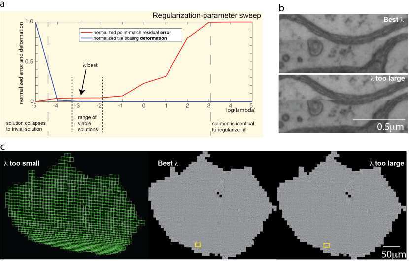
Figure 2: Choice of regularization parameter. (a–b) Parameter sweep (changing $\lambda$) for determining optimal range for regularization parameter value. (c) Examples of solutions for three cases of regularization parameter values ($\lambda$ too small, good, and too large) for a whole adult fruit fly section. (d) and (e) Visual comparison of stitching quality for cases between good regularization and excessive regularization. Images correspond to approximately same region (boxes above).

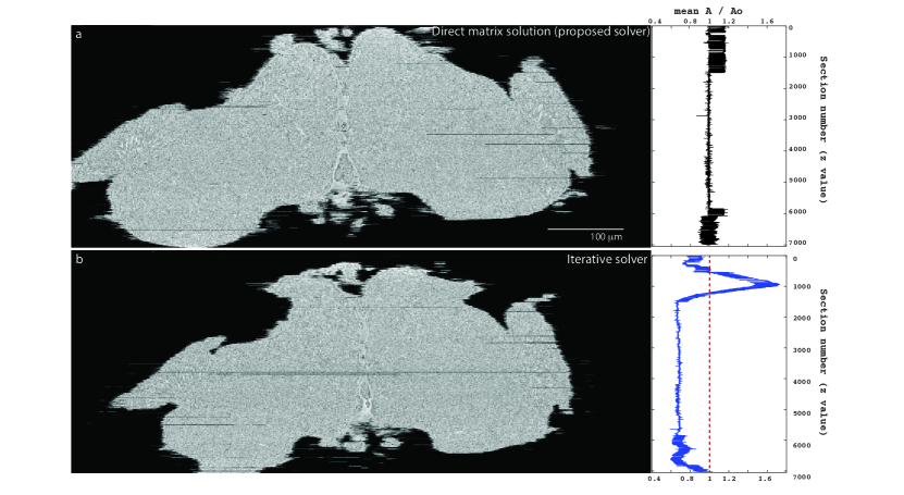
Figure 3: Comparison of direct matrix solver method with iterative solution by Scheffer et al. (2013). (a) The volume was subdivided into 78 contiguous overlapping slabs of approximately 250,000 tiles each. Slab overlap was 100 sections. Each slab was solved using Matlab’s backslash operator. Total matrix solution time $\approx 18$ hours using one Broadwell node with 32 CPUs; 576 CPU hours. Right panel shows deformation measure as ratio between tile area after optimization vs. original tile area for 7062 sections (b) Full system solve by iteratively updating transformations for each tile, solving a small affine system locally using the method in Scheffer et al. (2013). Total solution time 6 hours on 240 CPUs; 1,440 CPU hours. Right panel as in (a).

Figure 4: Nonlinear models are supported by the proposed joint-deformation solution method.

Supplementary Figure 1: Stitching of six tiles without regularization. Only term 1 in Equation 1 was constructed and solved. One tile, labeled “Fixed tile”, was used as reference.

Supplementary Figure 2: Necessity of regularization for large numbers of tiles. (a–c) 536 tiles of an adult fruit-fly section registered without regularization ($\lambda=0$), with insufficient, and with good regularization respectively. (d,e) zoomed-in view of region marked by yellow box in (c) for the initial guess (before stitching) and the regularized stitching result respectively.

Supplementary Figure 3: Typical workflow for serial section montaging and alignment.

References

- Bock et al. (2011) D. D. Bock, W.-C. A. Lee, A. M. Kerlin, M. L. Andermann, G. Hood, A. W. Wetzel, S. Yurgenson, E. R. Soucy, H. S. Kim, and R. C. Reid. Network anatomy and in vivo physiology of visual cortical neurons. Nature, 471:177–182, 2011. doi: doi:10.1038/nature09802.
- Bookstein (1989) F. L. Bookstein. Principal warps: thin-plate splines and the decomposition of deformations. IEEE Transactions on Pattern Analysis and Machine Intelligence, 11(6):567–585, 1989.
- Cardona et al. (2012) A. Cardona, S. Saalfeld, J. Schindelin, I. Arganda-Carreras, S. Preibisch, M. Longair, P. Tomančák, V. Hartenstein, and R. J. Douglas. Trakem2 software for neural circuit reconstruction. PLoS ONE, 7(6):e38011, 2012. doi: 10.1371/journal.pone.0038011.
- Golub and Loan (2013) G. Golub and C. V. Loan. Matrix Computations. The Johns Hopkins University Press, 2013.
- Hénon et al. (2002) P. Hénon, P. Ramet, and J. Roman. PaStiX: A High-Performance Parallel Direct Solver for Sparse Symmetric Definite Systems. Parallel Computing, 28(2):301–321, Jan. 2002.
- Karsh (2016) B. Karsh. Aligner for large scale serial section image data. GitHub repository, https://github.com/billkarsh/Alignment_Projects, 2016.
- Kaynig et al. (2010) V. Kaynig, B. Fischer, E. Müller, and J. M. Buhmann. Fully automatic stitching and distortion correction of transmission electron microscope images. Journal of Structural Biology, 171(2):163–173, 2010.
- Khairy (2018) K. A. Khairy. EM aligner. GitHub repository, https://github.com/khaledkhairy/EM_aligner, 2018.
- Lowe (2004) D. G. Lowe. Distinctive image features from scale-invariant keypoints. International Journal of Computer Vision, 60(2):91–110, 2004.
- Saalfeld et al. (2010) S. Saalfeld, A. Cardona, V. Hartenstein, and P. Tomančák. As-rigid-as-possible mosaicking and serial section registration of large sstem datasets. Bioinformatics, 26(12):i57–i63, 2010. doi: 10.1093/bioinformatics/btq219.
- Saalfeld et al. (2012) S. Saalfeld, R. Fetter, A. Cardona, and P. Tomančák. Elastic volume reconstruction from series of ultra-thin microscopy sections. Nature Methods, 9(7):717–720, 2012. doi: 10.1038/nmeth.2072.
- Schaefer et al. (2006) S. Schaefer, T. McPhail, and J. Warren. Image deformation using moving least squares. ACM Transactions on Graphics, 25(3):533–540, 2006. doi: http://doi.acm.org/10.1145/1141911.1141920.
- Scheffer et al. (2013) L. K. Scheffer, B. Karsh, and S. Vitaladevun. Automated alignment of imperfect em images for neural reconstruction. arXiv:1304.6034 [q-bio.QM], 2013.
- Takemura et al. (2015) S.-y. Takemura, C. S. Xu, Z. Lu, P. K. Rivlin, T. Parag, D. J. Olbris, S. Plaza, T. Zhao, W. T. Katz, L. Umayam, C. Weaver, H. F. Hess, J. A. Horne, J. Nunez-Iglesias, R. Aniceto, L.-A. Chang, S. Lauchie, A. Nasca, O. Ogundeyi, C. Sigmund, S. Takemura, J. Tran, C. Langille, K. Le Lacheur, S. McLin, A. Shinomiya, D. B. Chklovskii, I. A. Meinertzhagen, and L. K. Scheffer. Synaptic circuits and their variations within different columns in the visual system of drosophila. Proceedings of the National Academy of Sciences, 112(44):13711–13716, 2015. ISSN 0027-8424. doi: 10.1073/pnas.1509820112.
- Tasdizen et al. (2010) T. Tasdizen, P. Koshevoy, B. C. Grimm, J. R. Anderson, B. W. Jones, C. B. Watt, R. T. Whitaker, and R. E. Marc. Automatic mosaicking and volume assembly for high-throughput serial-section transmission electron microscopy. Journal of Neuroscience Methods, 193(1):132–144, 2010. doi: 10.1016/j.jneumeth.2010.08.001.
- ya Takemura et al. (2013) S. ya Takemura, A. Bharioke, Z. Lu, A. Nern, S. Vitaladevuni, P. K. Rivlin, W. T. Katz, D. J. Olbris, S. M. Plaza, P. Winston, T. Zhao, J. A. Horne, R. D. Fetter, S. Takemura, K. Blazek, L.-A. Chang, O. Ogundeyi, M. A. Saunders, V. Shapiro, C. Sigmund, G. M. Rubin, L. K. Scheffer, I. A. Meinertzhagen, and D. B. Chklovskii. A visual motion detection circuit suggested by Drosophila connectomics. Nature, 500:175–181, 2013. doi: 10.1038/nature12450.
- Zheng et al. (2017) Z. Zheng, J. S. Lauritzen, E. Perlman, C. G. Robinson, M. Nichols, D. Milkie, O. Torrens, J. Price, C. B. Fisher, N. Sharifi, S. A. Calle-Schuler, L. Kmecova, I. J. Ali, B. Karsh, E. T. Trautman, J. Bogovic, P. Hanslovsky, G. S. X. E. Jefferis, M. Kazhdan, K. Khairy, S. Saalfeld, R. D. Fetter, and D. D. Bock. A complete electron microscopy volume of the brain of adult drosophila melanogaster. bioRxiv, page 140905, 2017.