Smoke and Mirrors: Signal-to-Noise and Time-Reversed Structures
in Gamma-Ray Burst Pulse Light Curves

Abstract

We demonstrate that the ‘smoke’ of limited instrumental sensitivity smears out structure in gamma-ray burst (GRB) pulse light curves, giving each a triple-peaked appearance at moderate signal-to-noise and a simple monotonic appearance at low signal-to-noise. We minimize this effect by studying six very bright GRB pulses (signal-to-noise generally $>100$), discovering surprisingly that each exhibits complex time-reversible wavelike residual structures. These ‘mirrored’ wavelike structures can have large amplitudes, occur on short timescales, begin/end long before/after the onset of the monotonic pulse component, and have pulse spectra that generally evolve hard to soft, re-hardening at the time of each structural peak. Among other insights, these observations help explain the existence of negative pulse spectral lags, and allow us to conclude that GRB pulses are less common, more complex, and have longer durations than previously thought. Because structured emission mechanisms that can operate forwards and backwards in time seem unlikely, we look to kinematic behaviors to explain the time-reversed light curve structures. We conclude that each GRB pulse involves a single impactor interacting with an independent medium. Either the material is distributed in a bilaterally symmetric fashion, the impactor is structured in a bilaterally symmetric fashion, or the impactor’s motion is reversed such that it returns along its original path of motion. The wavelike structure of the time-reversible component suggests that radiation is being both produced and absorbed/deflected dramatically, repeatedly, and abruptly from the monotonic component.

1 Introduction

It has become apparent that pulses are the basic radiative units of gamma-ray burst (GRB) prompt emission (e.g., see Hakkila & Preece (2011); Hakkila et al. (2015, 2018) and references contained therein), containing key information about the physical mechanisms of GRBs and the environments in which they occur. However, GRB pulses do not conform to the standard definition of “single vibrations or short bursts of sound, electric current, light, or other waves” (Oxford English Dictionary).

Instead, a variety of observed properties characterize GRB pulses, including durations ranging from milliseconds to hundreds of seconds (Norris et al., 1996), longer decay times than rise times (pulse asymmetry) (Norris et al., 1996), longer durations at lower energies than at higher energies (Richardson et al., 1996), durations that anti-correlate with their peak fluxes (Hakkila & Preece, 2011), fluences that correlate with their durations (Hakkila & Preece, 2011), emissions that start nearly simultaneously in different energy bands (Hakkila & Nemiroff, 2009), hard-to-soft spectral evolution (Norris et al., 2005; Hakkila et al., 2015), more pronounced hard-to-soft evolution for hard asymmetric pulses than for soft symmetric ones (Hakkila et al., 2015, 2018), similar correlated behaviors regardless of the burst class to which they belong (long, intermediate, or short; Hakkila & Preece (2011); Hakkila et al. (2015, 2018)), and more symmetric, longer duration light curves at lower energies than at higher energies (Hakkila et al., 2015). Additionally, the interpulse separations in short GRBs increase with the durations of both the initial and subsequent pulses (Hakkila et al., 2018). This effect has not been apparent in long GRB pulses (Ramirez-Ruiz & Fenimore, 2000).

GRB pulses are non-monotonic in nature (Hakkila & Preece, 2014; Hakkila et al., 2015, 2018). They undergo brighter intensity fluctuations than are expected from only Poisson noise, and these fluctuations are in phase with the underlying monotonic pulse structure. The fluctuations are thus not indicative of noise, nor of isolated pulses, but rather of pulse components. This non-monotonicity is critically important in characterizing GRB pulses, because otherwise every observed non-stochastic fluctuation in a pulse light curve can be interpreted as being a separate pulse, leading to improper conclusions about the number of pulses, pulse characteristics, and inter-pulse separations. The most basic non-monotonic pulse fluctuations are smoothly-varying, triple-peaked structures that can be viewed by fitting a GRB pulse light curve with a monotonic function, subtracting the fit from the data, and examining the remaining pulse residuals. Although pulses generally exhibit hard-to-soft evolution, those with noticeable triple-peaked structures tend to undergo spectral re-hardening just before or at the time of a peak, and this can give some pulses (particularly those that are softer and more symmetric) the appearance of having intensity-tracking spectral evolution. Although some pulses exhibit smooth monotonic or triple-peaked structures, others exhibit more complex, chaotic structures that are often particularly noticeable at higher energies. Pulses observed in noisy data show little structure and are best described as monotonic.

We use the word structure to describe variations exceeding those commonly expected from a monotonic GRB pulse light curve. This structure definition refers to any intensity variation that results in an inadequate monotonic fit to an otherwise distinct emission episode. As such, it is instrument-dependent, because bright GRB pulses often exhibit structure whereas faint pulses rarely do. We have recently developed a classification scheme for Short GRB pulses (Hakkila et al., 2018) which demonstrates that the amount of structure in GRB pulses increases as the signal-to-noise ($S/N$) increases, and as the temporal bin size decreases. In other words, structure seems to be an inherent feature of GRB pulses that is not always apparent in data because it can get washed out by instrumental effects.

Structure is less pronounced in faint GRB pulses than in bright ones (Hakkila & Preece, 2014; Hakkila et al., 2015, 2018), and $S/N$ plays an important role in this. Signal-to-noise can decrease for a variety of instrumental reasons, including inefficient photon detection, small detector surface area, decreased temporal bin size, decreased spectral range, increased spectral resolution, and detection at lower (noisier) energies. It seems intuitively obvious that structure and noise should become indistinguishable from one another when they have comparable amplitudes. However, structure and an underlying smooth pulse profile are both present in light curves of GRB pulses. As signal-to-noise decreases, does structure disappear before or after the smoothly-varying remainder of the pulse disappears? How does this affect the properties of pulses measured at low signal-to-noise relative to those at high signal-to-noise? Is it possible that other pulse properties might accompany these changes at low signal-to-noise (e.g., duration, asymmetry, and spectral evolution), and what might such changes, if observed, tell us about the influence of instrumental biases on GRB pulse measurements?

We wish to explore these questions further using pulses from bright Long GRBs observed by BATSE (the Burst And Transient Source Experiment; Horack (1991)) on NASA’s Compton Gamma Ray Observatory (CGRO). BATSE had one of the largest surface areas of any GRB experiment and thus was able to observe many GRBs at large $S/N$ ratios.

2 Empirical Pulse and Residual Model

2.1 The Pulse Model

In order to explore structure as a function of $S/N$, we must first define and characterize structureless pulses. We do this by using the monotonic asymmetric intensity function of Norris et al. (2005):

$$I(t)=A\lambda e^{[-\tau_{1}/(t-t_{s})-(t-t_{s})/\tau_{2}]},$$ (1)

where $t$ is time since trigger, $A$ is the pulse amplitude, $t_{s}$ is the pulse start time, $\tau_{1}$ is the pulse rise parameter, $\tau_{2}$ is the pulse decay parameter, and the normalization constant $\lambda$ is $\lambda=\exp{[2(\tau_{1}/\tau_{2})^{1/2}]}$. The intensity is the count rate obtained from the total counts observed in BATSE energy channels 1 ($20-50$ keV), 2 ($50-100$ keV), 3 ($100-300$ keV), and 4 (300 keV $-1$ MeV) at 64 ms temporal resolution. Poisson statistics and a two-parameter background counts model of the form $B=B_{0}+BS\times t$ are assumed (where $B$ is the background counts in each bin and $B_{0}$ and $BS$ are constants denoting the mean background (counts) and the rate of change of the mean background (counts/s)). This model can be used to produce observable pulse parameters such as pulse peak time ($\tau_{\rm peak}=t_{s}+\sqrt{\tau_{1}\tau_{2}}$), pulse duration ($w$) and pulse asymmetry ($\kappa$). As a result of the smooth rapid rise and more gradual fall of the pulse model, $w$ and $\kappa$ are measured relative to some fraction of the peak intensity. Following (Hakkila & Preece, 2011), we measure $w$ and $\kappa$ at $I_{\rm meas}/I_{\rm peak}=e^{-3}$ (corresponding to $0.05I_{\rm peak}$), or

$$w=\tau_{2}[9+12\mu]^{1/2},$$ (2)

where $\mu=\sqrt{\tau_{1}/\tau_{2}}$, and

$$\kappa\equiv[1+4\mu/3]^{-1/2}.$$ (3)

Asymmetries range from symmetric ($\kappa=0$ when $\tau_{1}\gg\tau_{2}$ and $\mu\rightarrow\infty$) to asymmetric ($\kappa=1$ when $\tau_{1}\ll\tau_{2}$ and $\mu\rightarrow 0$) with longer decay than rise times.

2.2 The Residual Model

Residuals to the Norris et al. (2005) model are generated by obtaining the best monotonic pulse fit for the observed pulse light curve and subtracting this fit from the data. Small yet distinct deviations in the residuals are found to be systematically in phase with the monotonic light curve (Hakkila & Preece, 2014), and these deviations are needed to accurately describe GRB pulse shapes. Although the deviations are closely aligned with the pulse duration, they are not always contained within it. Thus we have defined a larger fiducial time interval $w_{\rm f}$ as

$$w_{\rm f}=t_{\rm end}-t_{\rm start}=4.4\tau_{2}(\sqrt{1+\mu/2}+1)+\sqrt{\tau_{1}\tau_{2}},$$ (4)

with the fiducial end time $t_{\rm end}$ given by

$$t_{\rm end}=\frac{w}{2}(1+\kappa)+t_{s}+\tau_{\rm peak}$$ (5)

and the fiducial start time $t_{\rm start}$ given by

$$t_{\rm start}=t_{s}-0.1[\frac{w}{2}(1+\kappa)-\tau_{\rm peak}].$$ (6)

The fiducial time interval is a unitless interval introduced to demonstrate the generic nature of GRB pulse residual structures, regardless of the durations and asymmetries of the underlying pulses containing them. Residuals are obtained using this time interval so that normalized pulse residual structures can be directly compared with one another, and so that goodness-of-fit measurements used in making these comparisons are not based on the amount of background sampled. The residuals exhibit variations that can be fitted with an empirical function (Hakkila & Preece, 2014) in the fiducial time interval f where $0\leq t^{\prime}\leq 1$:

$$\textrm{res($t^{\prime}$)}=\left\{\begin{array}[]{ll}aJ_{0}(\sqrt{\Omega_{\rm f}[t_{\rm 0;f}-t^{\prime}-0.005]})&\textrm{if $t^{\prime}<t_{\rm 0;f}-0.005$}\\ a&\textrm{if $t_{\rm 0;f}-0.005\leq t^{\prime}\leq t_{\rm 0;f}+0.005$}\\ aJ_{0}(\sqrt{s_{\rm f}\Omega_{\rm f}[t^{\prime}-t_{\rm 0;f}-0.005]})&\textrm{if $t^{\prime}>t_{\rm 0;f}+0.005$.}\end{array}\right.$$ (7)

Here, $J_{0}(x)$ is an integer Bessel function of the first kind, $t_{\rm 0;f}$ is the unitless time of the residual peak, $a_{\rm f}$ is the amplitude of the residual peak, $\Omega_{\rm f}$ is the unitless Bessel function’s angular frequency that defines the timescales of the residual wave (a large $\Omega_{\rm f}$ corresponds to a rapid rise and fall), and $s_{\rm f}$ is a dimensionless scaling factor that relates the fraction of time which the function pre-$t_{\rm 0;f}$ has been compressed relative to its time-inverted form post-$t_{\rm 0;f}$. The time during which the pulse intensity is a maximum is required to be a plateau instead of a peak because otherwise the width of the Bessel function’s first lobe would not be broad enough to capture the extent of the central peak. Therefore, a duration of $w_{\rm plateau}\approx 0.010w_{\rm fid}$ is hard-coded into the fitting routine to create a small plateau structure in the function. Without evidence in the pulse shape that the Bessel function continued beyond the third zero (following the second half-wave), Hakkila & Preece (2014) truncated the function at the third zero $J_{0}(x=\pm 8.654)$, giving the fitting function a triple-peaked appearance. Because the central plateau most commonly aligns with the peak of the monotonic pulse, the three residual function peaks were named the precursor peak, the central peak, and the decay peak, respectively (Hakkila & Preece, 2014).

In some pulses the central peak of the residual function does not closely align with the peak of the monotonic pulse (see Hakkila et al. (2018) and Section 4 of this manuscript). The reason for this misalignment is still not well-understood but it appears to signify that the residual function and the monotonic function are separate pulse components.

After fitting, the unitless fiducial values are converted back to the observed time interval using:

$$a=a_{\rm f}$$ (8)

$$s=s_{\rm f},$$ (9)

$$t_{0}=t_{\rm 0;f}(t_{\rm end}-t_{\rm start})+t_{\rm start},$$ (10)

and

$$\Omega=\Omega_{\rm f}/(t_{\rm end}-t_{\rm start}),$$ (11)

where $t_{\rm start}$ and $t_{\rm end}$ are the real time values corresponding to the start and end of the fiducial time interval. The Bessel function frequency $\Omega$ is now given in units of $s^{-1}$ and the residual peak time $t_{0}$ is now given in units of $s$.

The flux contribution that the residual function makes to the combined pulse fit, as well as its relative temporal alignment, is capable of significantly altering a pulse shape from that of monotonicity. Although the precursor peak and the decay peak of the residual function typically fall during the rise and decay portions of the monotonic fitting function, in some cases the precursor peak can occur before the formal rise of the monotonic pulse. When the precursor peak is harder than the central peak, the hard-to-soft pulse evolution is pronounced. When the precursor peak is softer than the central peak, the pulse begins evolving hard-to-soft but then re-hardens to a maximum value around the time of the central peak, and the pulse hardness appears to track with intensity. Additionally, the central residual peak and the peak of the monotonic pulse do not always align with one another, producing an extra smooth pulse structure in some cases.

The 64 ms $S/N$ is a measure of the peak brightness of each GRB, relative to its background count measured with 64 ms temporal resolution. The $S/N$ is

$$S/N=(P_{64}-B)/\sqrt{P}_{64},$$ (12)

where $P_{64}$ is the 64 ms peak counts and $B$ is the mean background count. This signal-to-noise ratio is primarily appropriate when analyzing GRB pulses fit on the 64 ms time scale.

Using the approach of Hakkila et al. (2018), we classify GRB pulses based on the amount of structure they exhibit, as defined relative to the $\chi^{2}_{\nu}$ $p-$values of the pulse fits. This method first fits each pulse with the monotonic Norris et al. (2005) fitting function and analyzes the goodness-of-fit with a $\chi^{2}-$test. We define $\chi^{2}$ over the fiducial timescale and $\nu$ from the Norris et al. (2005) model as the number of temporal bins minus the number of pulse- and background-fit parameters – two for the background and four for a single pulse. The $p-$value associated with $\chi^{2}_{\nu}$ is the probability that a value of $\chi^{2}$ or less having $\nu$ degrees of freedom will be measured in a random distribution. We consider good fits (indicating relatively smooth light curves) to be those having standard best-fit $p-$values of $p_{\rm best}\geq 5\times 10^{-3}$. Next, this monotonic pulse fit is subtracted from the light curve leaving a residual light curve. The residual light curve is then fitted with the Hakkila & Preece (2014) residual fitting model. Finally the residual fit is added to the monotonic pulse fit to produce a total fit, and this is tested to see whether or not adding the residual fitting function significantly improved the overall pulse fit. A $\Delta\chi^{2}$ test is used to indicate whether or not the residual function should be included in the fit: $\Delta\chi^{2}$ is the difference in $\chi^{2}$ obtained from the Norris et al. (2005) model minus that obtained from the Norris et al. (2005) model combined with the Hakkila & Preece (2014) residual model. The difference in the number of degrees of freedom between these fits is four for a single pulse. If adding the residual fit significantly improved the pulse fit, then the combined models act as the pulse fit. But if the addition of the residual fit does not improve the overall pulse fit, then only the original monotonic pulse fit is used to represent the final pulse fit. We require a $\Delta\chi^{2}$ $p-$value of $p_{\Delta}\leq 10^{-3}$ for the model to be considered significantly improved and therefore use the combined pulse models to represent the final pulse fit.

We use this approach to classify GRB pulses into one of four groups. Simple pulses are those best characterized by Equation 1 alone ($p_{\rm best}\geq 5\times 10^{-3}$). Blended pulses are fits improved using Equation 7 ($p_{\Delta}\leq 10^{-3}$ and $p_{\rm best}\geq 5\times 10^{-3}$). Structured pulses have many characteristics that can be explained by the pulse and residual models, but also have significant deviations from these structures ($p_{\Delta}\leq 10^{-3}$ and $10^{-5}\leq p_{\rm best}<5\times 10^{-3}$). Complex pulses have complicated light curves ($p_{\rm best}<10^{-5}$).

3 Analysis

We hypothesize that bright, complex GRB emission episodes are really structured pulses that can be reduced to triple-peaked and monotonic shapes with the loss of $S/N$. We test this hypothesis by analyzing four of BATSE’s brightest GRBs. Specifically, we study BATSE triggers 143 (GRB 910503), 249 (GRB 910601), 5614 (GRB 960924), and 7301 (GRB 990104B) (Paciesas et al., 2000). All four bursts have been observed in BATSE energy channels $1-4$ (20 keV to 1 MeV) with 64 ms temporal resolution. We initially limited our sample to five pulses with $S/N>100$. However, because BATSE 7301 contains two bright pulses, we also chose to analyze the second pulse of BATSE 143 ($S/N=55.9$) for completeness. As we will show in Section 3.1.1, any pulse with $S/N>25$ can be considered to be “bright” for the purposes of this analysis.

BATSE trigger 143 contains two distinct emission episodes peaking at $1.7$ seconds and 48 seconds after the trigger. The brighter first event (143p1) has a $S/N=131.5$, a duration of $w=9.9$ seconds, an asymmetry of $\kappa=0.75$, and has considerable temporal structure, while the smoother and fainter second event (143p2) has $S/N=55.9$, $w=11.2$ seconds, $\kappa=0.59$, and shows clear evidence of the triple-peaked structure.

BATSE trigger 249 is a complex, time-symmetric emission episode with $S/N=108.0$ peaking $21.9$ seconds after the trigger and containing at least 5 separate emission peaks. The entire episode lasts some 38 seconds, although the fitted pulse lasts only $w=20.8$ seconds and has an asymmetry of $\kappa=0.07$.

BATSE trigger 5614 is a bright ($S/N=177.2$) single-peaked asymmetric emission episode ($\kappa=0.69$) peaking $8.4$ seconds after the trigger with a duration of $w=6.7$ seconds. Although the burst has the appearance of a fairly smooth single pulse, the main part of the pulse rise does not occur until roughly 7 seconds after the trigger. Of the six pulses in the sample, this one most clearly exhibits the triple-peaked pulse shape described in previous papers.

BATSE trigger 7301 is a complex burst with what appear to be four separate complex emission episodes. For reasons we will discuss later, we identify only the two brightest episodes as pulses 7301p1 and 7302p2 (these peak $15.8$ seconds and $165.1$ seconds after the trigger, respectively) while excluding the fainter emission episodes starting at the trigger ($t=0$ seconds) and at around $t=32$ seconds. Pulse 7301p1 is a bright, complex episode with $S/N=100.9$, $w=10.7$ seconds and $\kappa=0.51$. Pulse 7301p2 is a bright, complex episode with $S/N=144.3$, $w=29.3$ seconds and $\kappa=0.52$; the pulse contains three bright peaks each lasting a few seconds which occur during fainter emission lasting roughly 50 seconds.

We initially assume that each of the bright, complex emission episodes in BATSE triggers 143, 249, 5614, and 7301 is composed of a single structured pulse. This is completely antithetical to the standard pulse-fitting approach in which each pulse would be treated as a light-curve variation that could not be attributed to noise. Using such an approach, 143p1, 249, 7301p1, and 7301p2 would be best fit by dozens of pulses. Even the apparently smoothly-varying 143p2 and 5614 would consist of at least half a dozen pulses because the burst is so structured at this $S/N$ level.

Fits to the six pulses using the monotonic model described by Equation 1 and the residual model described by Equation 7 are shown in Figures 1 $-$ 6. The left panels of Figures 1 $-$ 6 show the residual structure while the right panels show both the monotonic fit (dotted line) and the combined fit (solid line). Each pulse is classified as complex using the formal criteria described in Section 2.2, indicating that the combination of the monotonic pulse model and the residual model do not adequately describe the pulse light curves. However, in each case it can be seen that the models contribute to only an approximate first-order fit by creating envelopes that contain the most noticeable structures, and that the residual fits are only rough approximations to the actual residual structure.

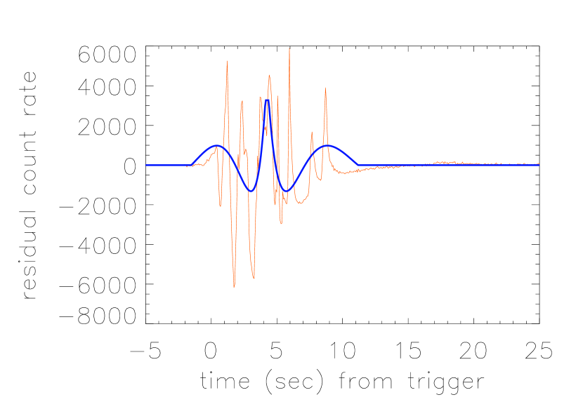
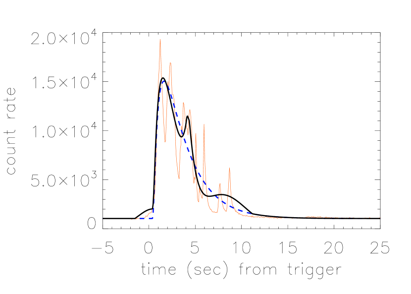
Figure 1: BATSE trigger 143p1 observed at $S/N=131.5$. The left panel shows the Hakkila & Preece (2014) residual structure, while the right panel shows both the Norris et al. (2005) pulse fit (dotted line) and the combined Norris et al. (2005) pulse plus Hakkila & Preece (2014) residual fit (solid line). In this and all subsequent plots, ‘residual count rate’ and ‘count rate’ refer to the number of counts per 64 ms bin.

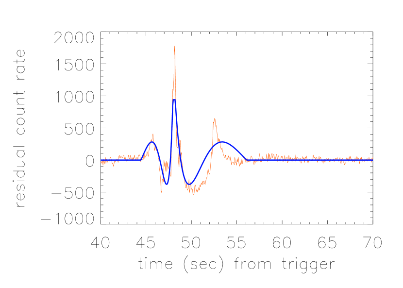
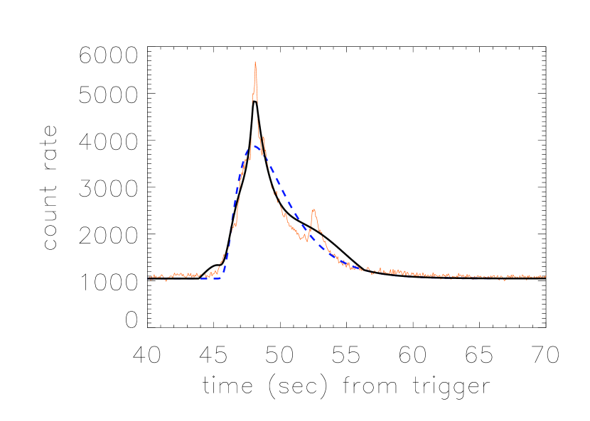
Figure 2: BATSE trigger 143p2 observed at $S/N=55.9$. The left panel shows the Hakkila & Preece (2014) residual structure, while the right panel shows both the Norris et al. (2005) pulse fit (dotted line) and the combined Norris et al. (2005) pulse plus Hakkila & Preece (2014) residual fit (solid line).

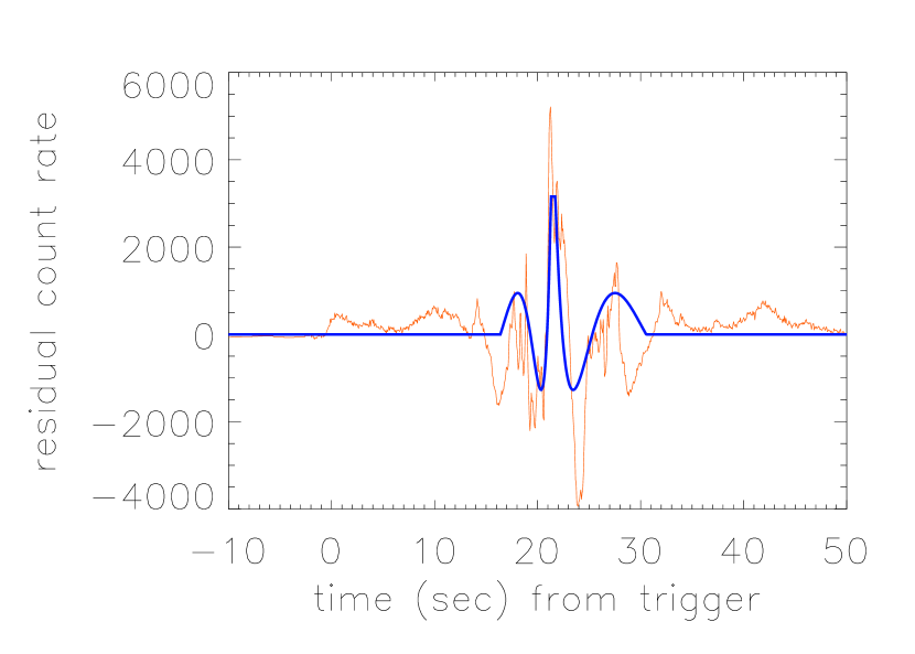
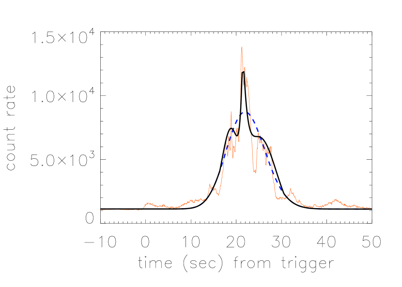
Figure 3: BATSE trigger 249 observed at $S/N=108.0$. The left panel shows the Hakkila & Preece (2014) residual structure, while the right panel shows both the Norris et al. (2005) pulse fit (dotted line) and the combined Norris et al. (2005) pulse plus Hakkila & Preece (2014) residual fit (solid line).

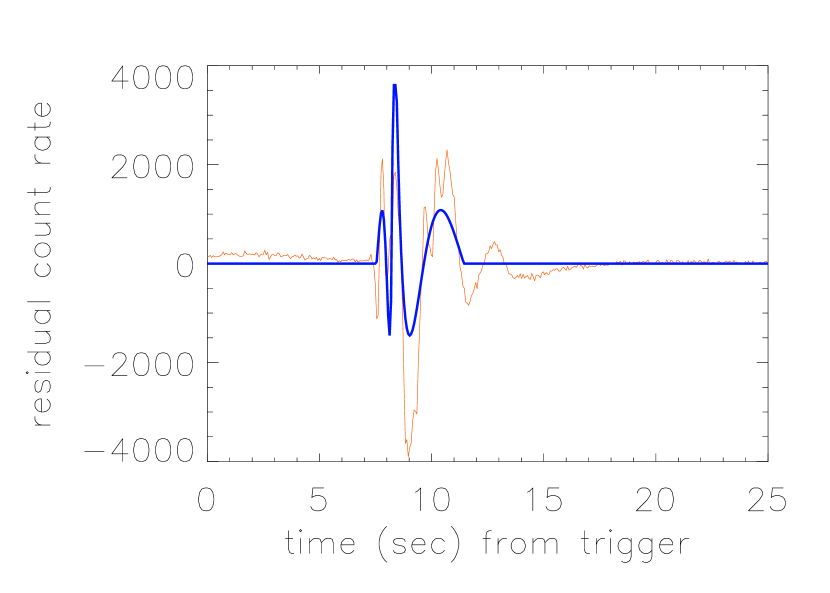
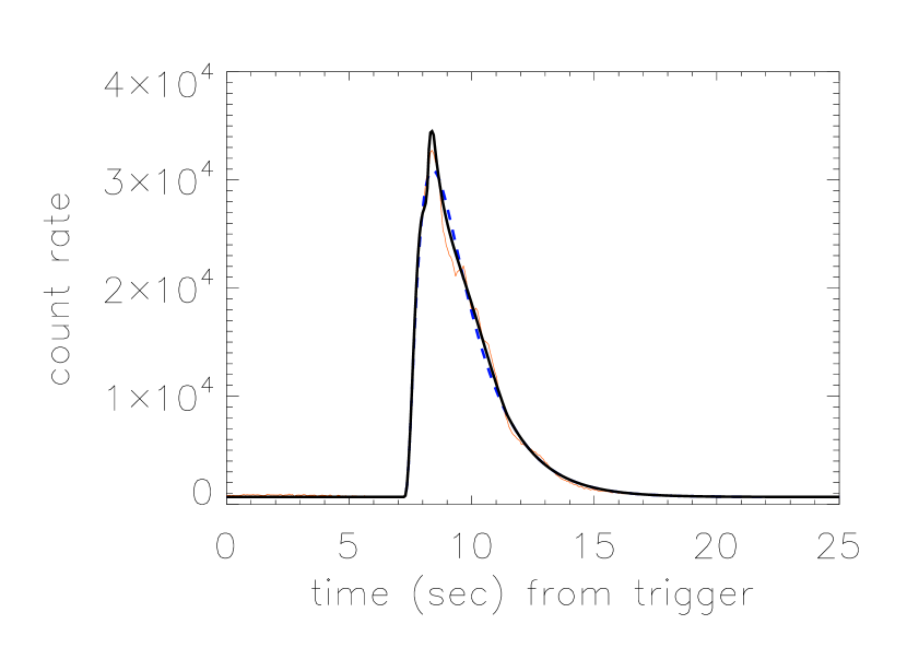
Figure 4: BATSE trigger 5614 observed at $S/N=177.2$. The left panel shows the Hakkila & Preece (2014) residual structure, while the right panel shows both the Norris et al. (2005) pulse fit (dotted line) and the combined Norris et al. (2005) pulse plus Hakkila & Preece (2014) residual fit (solid line).

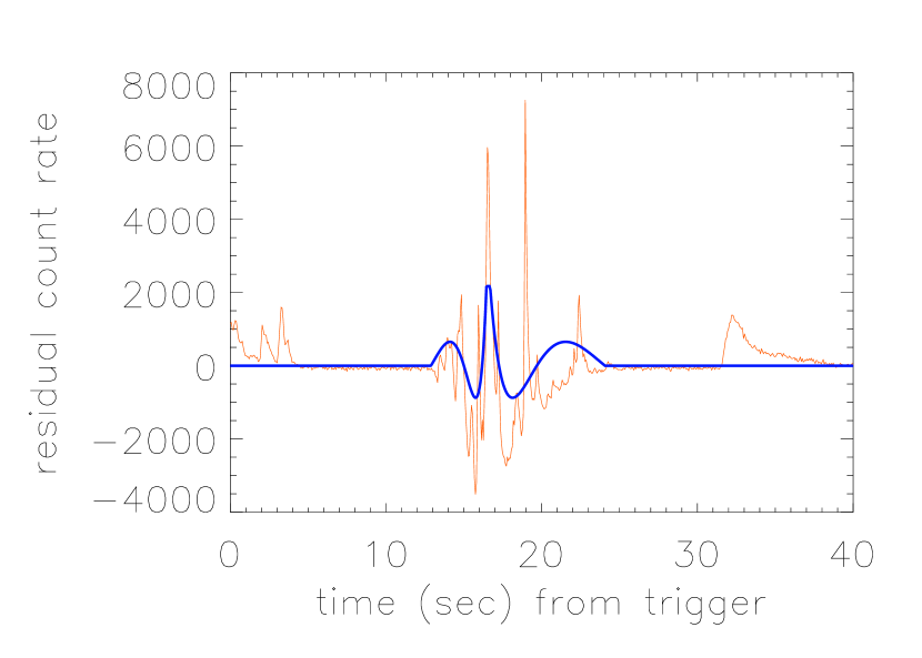
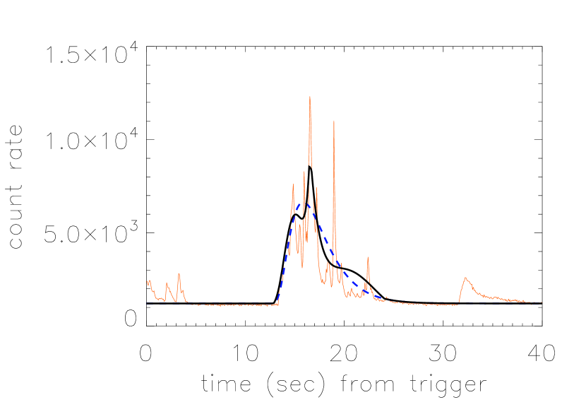
Figure 5: BATSE trigger 7301p1 observed at $S/N=100.9$. The left panel shows the Hakkila & Preece (2014) residual structure, while the right panel shows both the Norris et al. (2005) pulse fit (dotted line) and the combined Norris et al. (2005) pulse plus Hakkila & Preece (2014) residual fit (solid line).

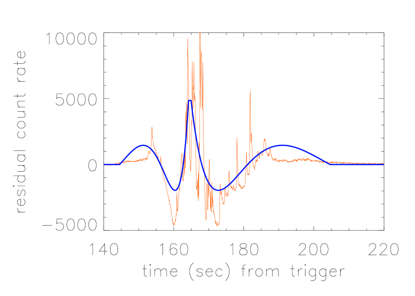
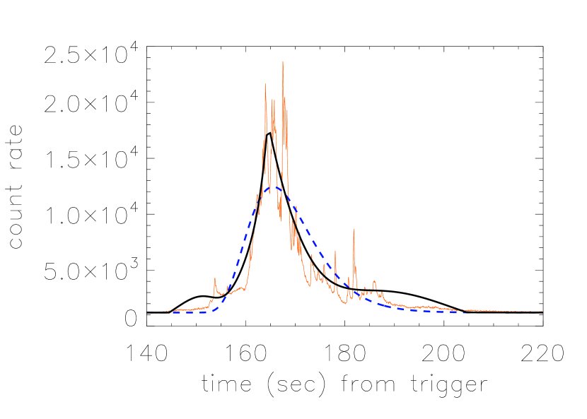
Figure 6: BATSE trigger 7301p2 observed at $S/N=144.3$. The left panel shows the Hakkila & Preece (2014) residual structure, while the right panel shows both the Norris et al. (2005) pulse fit (dotted line) and the combined Norris et al. (2005) pulse plus Hakkila & Preece (2014) residual fit (solid line).

3.1 Smoke: Pulse Properties as Functions of Signal-to-Noise

We estimate the properties of these six BATSE pulses at lower $S/N$ by reducing their assumed “intrinsic” counts distributions and adding stochastic instrumental noise. The pulse plus residual fits described thus far have been based on the summed counts in BATSE’s four energy channels $1+2+3+4$. Since some pertinent pulse properties are energy-dependent (e.g., spectral lags), we use a process that produces reductions in each individual energy channel rather than only in the summed four-channel light curve.

For each of the six BATSE pulses listed, we estimate their properties at lower $S/N$ values by removing the background from each energy channel and assuming that the remaining photon flux distribution is a fair representation of the “intrinsic” flux distribution. When summed together, these channel-dependent counts allow us to reproduce the “intrinsic” summed four-channel counts observed by the instrument. We then define roughly ten equal logarithmic four-channel count intervals between the observed peak count rate and a measure close to background (ostensibly near $S/N\approx 3$). For each energy channel we iteratively decrease the peak counts proportionally through these logarithmic decrements, add energy-dependent Poisson noise to the results, and recombine the energy channel-dependent light curves to obtain a reduced-intensity four-channel light curve.

This process assumes that the reduced pulse would have been detected with a similar background rate if it had been detected at a lower $S/N$, an assumption that is only partially valid because the background rate varied slowly and regularly throughout the Compton Gamma-Ray Observatory’s mission in response to the satellite’s eccentric orbit. The “noisification” process also assumes that there is no systematic coupling between detector energy channels, and that the detector response does not depend significantly on count rate. There are potential problems with both of these assumptions: the non-diagonal energy response of BATSE’s Large Area Detectors (LADs) created a coupling between energy channels, and low $S/N$ observations were affected by spacecraft orientation and relative direction between the Earth and a GRB (e.g., see Pendleton et al. (1996)). However, we believe that both assumptions are valid as first-order approximations.

3.1.1 Pulse Structure

As $S/N$ decreases, pulse structure becomes less noticeable. At high $S/N$, pulse structure is easily distinguishable and separable from Poisson noise. At low $S/N$, structure becomes indistinguishable from noise, while the underlying smooth monotonic pulse remains identifiable and measurable. This becomes an issue when determining the number of pulses potentially present in a GRB light curve: at low $S/N$ the monotonic pulse dominates over structure, and the light curve appears to be that of a single pulse. At moderate and high $S/N$ these structures are clearly not the result of noise, and can even appear to be so pronounced that they can be mistaken for separate pulses. However, confusion in the number of pulses can be reduced by recognizing that the structures are linked in phase with the main body of emission, either sitting atop the monotonic pulse (e.g., 143p1; see Figure 1) or a connected to it as a continuum of episodes like cutout paper doll chains (e.g., 249; see Figure 3). The importance of this relationship will be discussed further in Section 4.

Figure 7 demonstrates two stages in the intensity reduction of BATSE trigger 249. If this pulse had been detected at $S/N=5.2$ (left panel), then it would be classified as blended because both monotonic and residual pulse models are needed to completely account for the pulse light curve variations. If the pulse had been detected at $S/N=4.3$ (right panel), then a fit to the residual function would not be statistically significant (as measured by $p_{\Delta}$) and the pulse would be classified as simple.

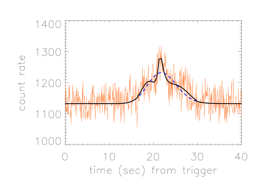
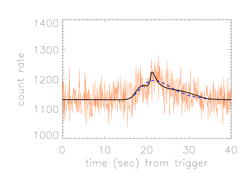
Figure 7: Two stages in the intensity reduction of 249. The left panel shows what the pulse can look like at $S/N=5.2$, where the pulse and residual fits combine to place the pulse in the blended class. The right panel shows what the pulse can look like at $S/N=4.3$, where the residuals do not statistically improve the fit and the pulse is classified as a simple pulse. Although the addition of the residual function does not significantly improve the fit at $S/N=4.3$, the combined pulse and residual fits are shown for visual comparison.

Figure 8 summarizes the effect of $S/N$ on pulse classification for the pulses in this study. All pulses are classified as complex at high $S/N$, and all pulses are classified as simple at low $S/N$. The $S/N$ values at which these transitions occur (complex to structured, structured to blended, and blended to simple) vary from pulse to pulse depending on the intrinsic pulse structure, the background at the time the burst was detected, and the way in which the random background fluctuations have interacted with the reduced pulse.

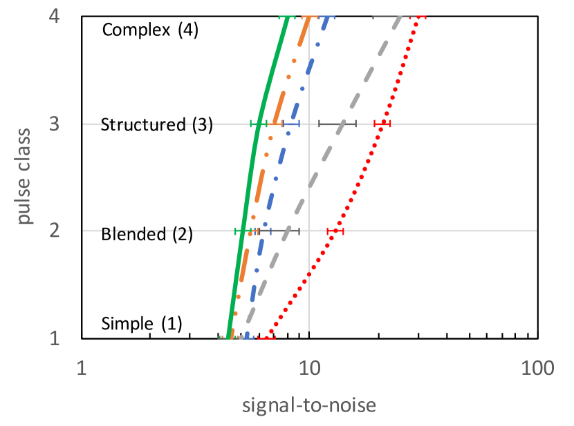
Figure 8: GRB pulse classification as $S/N$ is reduced. Indicated are the general paths taken during $S/N$ reduction by each of the five pulses shown: 5614 (red dotted line), 143p1 (blue dashed-dotted line), 143p2 (gray dashed line), 249 (orange dashed-double-dotted line), and 7301p1 (green solid line). The reduced classification of 7301p2 is not plotted, but is similar to that of 249. Simple pulses (class 1) are best characterized by monotonic pulses, blended pulses (class 2) are best characterized by a monotonic pulse overlaid by a smooth triple-peaked residual function, structured pulses (class 3) are improved but not adequately characterized by a pulse plus the residual function, and complex pulses (class 4) are too structured to be described by these simple pulse models.

It is useful to compare the $S/N$ distributions of pulses populating each class to the overall pulse $S/N$ distribution. To do this we must estimate the numbers of pulses in each class because each pulse must be fitted before it can be classified, and this is a time-consuming procedure. Even estimating the overall pulse $S/N$ distribution must be performed with care because measuring the mean background for each burst first requires us to separate the background from the pulse (and from multiple pulses when the burst contains more than one); this again requires us to fit each pulse before we can characterize its $S/N$.

In order to carry out our estimate we first note that there is a strong correlation between $S/N$ values and published BATSE 1024 ms $C_{\rm max}/C_{\rm min}$ values (the count rate at which a GRB triggers relative to the minimum count rate for a trigger to occur):

$$S/N=4.606(C_{\rm max}/C_{\rm min})^{0.669},$$ (13)

with a correlation coefficient of $R^{2}=0.933$. From this correlation we can estimate the $S/N$ distribution of the brightest pulses in each BATSE burst using $C_{\rm max}/C_{\rm min}$ (again, we cannot identify the $S/N$ distribution of all pulses without going through the time-consuming process of fitting all pulses). Second, we obtain the distribution of BATSE GRB pulses fitted in previous papers (e.g., Hakkila & Preece (2014); Hakkila et al. (2015)). We make sure to exclude GRBs with $T_{90}$ durations less than 2 seconds ($T_{90}$ is the duration spanned by 90% of the flux) because 64 ms binning distorts any structure present; Hakkila et al. (2018)). We overlay the estimated pulse distribution with the observed distributions of simple, blended, structured, and complex pulses in Figure 9. It is apparent that the current fitted pulse distribution favors pulses exhibiting the triple-peaked structure (e.g., blended and structured) because of our bias towards looking for evidence of it.

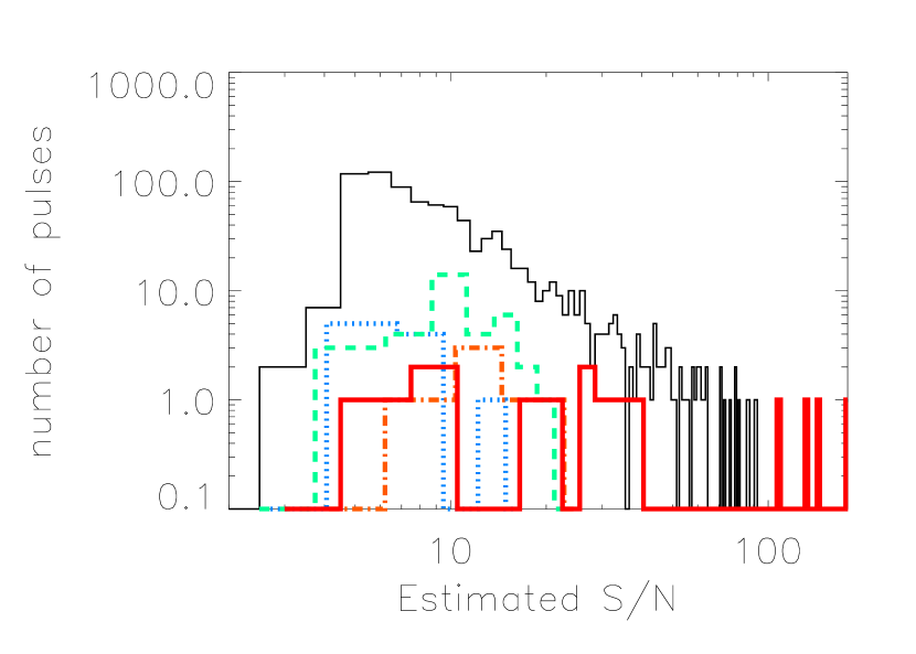
Figure 9: The estimated $S/N$ distribution of the brightest BATSE pulse in each burst (solid black line). The plot is overlaid with the measured $S/N$ values of classified BATSE pulses (primarily from Hakkila & Preece (2014); Hakkila et al. (2015)) Simple pulses (blue dotted line) are found at the lowest $S/N$ ($\langle\log(S/N)\rangle=0.83$ or $S/N=6.7$), blended pulses (dashed green line) have ($\langle\log(S/N)\rangle=1.03$ or $S/N=10.7$), structured pulses (dotted-dashed orange line) have ($\langle\log(S/N)\rangle=1.15$ or $S/N=14.1$), and complex pulses (solid red line) have ($\langle\log(S/N)\rangle=1.51$ or $S/N=32.7$). The large $S/N$ of the pulses in this sample ($S/N>100$) can be contrasted with the rest of the distribution. Note also that all pulses with $S/N\geq 25$ have been classified as complex.

Based on the classification criteria of these pulses and on the distribution of BATSE pulse $S/N$ values, we estimate that at least $50\%$ of pulses from long BATSE GRBs are found at $S/N\leq 8$. Most of these are likely to be classified as either simple or blended, although pulses containing more structure are also found at these $S/N$ values. This result explains both why Hakkila & Preece (2014) were able to establish a simple residual model using low-$S/N$ pulses and why the residual model did not suffice when applied to bright pulses. It is entirely likely that all GRB pulses exhibit complex structures, but only a small fraction of pulses exhibit these structures without having them smoothed by instrumental effects related to $S/N$.

However, caution must be exerted in generalizing and interpreting why GRB pulse structure exists at low $S/N$. Not all faint pulses are simple; some have been classified as blended, structured, and even complex. Smeared-out, complex, intrinsic pulse structures can appear indistinguishable from overlapping pulses at low $S/N$.

3.1.2 Pulse Duration and Asymmetry

Although observing a GRB pulse at reduced $S/N$ smears out its pulse structure, the pulse’s duration ($w$) and asymmetry ($\kappa$) extracted from the monotonic model shown in Equation 1 do not appear to be systematically affected. Figure 10 demonstrates this for the bright pulses in this sample as $S/N$ is reduced. Measured $w$ and $\kappa$ values are, however, affected statistically by large uncertainties at low $S/N$ ($S/N<6$). We also note that the pulses with the largest amounts of structure preceding and following the main monotonic component (249, 7301p1, and 7301p2) have the largest duration and asymmetry uncertainties at all $S/N$ values. Pulses in which structure overlays the monotonic component (143p1, 143p2, and 5614) have smaller uncertainties that actually serve to guide the monotonic pulse fit and decrease uncertainty in measuring the pulse fit parameters ($\tau_{1}$, $\tau_{2}$, $t_{s}$, and $A$).

Figure 10: Fitted durations (left panel) and asymmetries (right panel) of pulses 143p1 (plusses), 143p2 (crosses), 249 (triangles), 5614 (diamonds), 7301p1 (asterisks), and 7301p2 (squares) as their $S/N$ values are reduced. Fitted pulse durations and asymmetries do not change systematically with decreased $S/N$, with the exception of 7301p2 (due to insufficient contributions to the fit from the loss of emission in the pulse’s broad “wings”). Some measurements appear to undergo discontinuous shifts as $S/N$ drops; this happens when pulse structure abruptly disappears into the noise and the fit parameters have to fit a more simply-structured pulse. Uncertainties increase for all pulse measurements when $S/N<6$.

3.1.3 Pulse Spectral Lags

Spectral lags indicate the time difference between the optimal alignment of pulse’s high-energy and low-energy fluxes. Lags are measured using the cross-correlation function (CCF). The CCF is either applied to the data (data lag); e.g., Cheng et al. (1995); Norris et al. (1996); Band (1997)) or to the fitted pulses (fit lag; Norris et al. (2005); Hakkila & Preece (2011)). Spectral lags correlate with GRB luminosity (Norris et al., 1996) and provide a simple measurement of spectral properties. Although there appears to be a general relationship between both types of lag and pulse evolution (e.g., Kocevski et al. (2003); Schaefer (2004); Ryde (2005); Hakkila & Preece (2011); Hakkila et al. (2015, 2018)), some pulses have negative data lags (Ukwatta et al., 2010; Roychoudhury et al., 2014; Chakrabarti et al., 2018) and data lags are often inconsistent with fit lags (e.g., Ukwatta et al. (2010)).

We predict that data lags obtained from structured pulse data will be different than fit lags of the same pulses. Short-duration pulses have shorter lags (of both types) than long-duration pulses (e.g., Norris et al. (2005); Peng et al. (2007); Hakkila et al. (2008)). This is not terribly surprising since a pulse’s lag must be shorter than the pulse’s duration since the flux distributions generally overlap (Hakkila & Preece, 2011). Similarly, structured pulses must have short data lags, since structure often occurs on short timescales, and since structure is generally bright enough to contribute significantly to the CCF peak. Fit lags measured by applying the CCF to multi-channel Norris et al. (2005) pulse fits, however, are not constrained to be short, because the fits effectively smear out any energy-dependent structures by redistributing them. Since the broad CCF distributions made from these smeared light curves smoothly span the entire pulse duration, the extracted fit lags can exceed the timescales of the structures. Additionally, pronounced structure in one energy channel but not another can shift the CCF, and therefore the lag obtained from it.

We calculate the data lags from the CCF for several energy channels for each pulse, and compare these to the lags of the smooth fitted monotonic pulse components (fit lags), the results of which can be found in Table 1. We have chosen to demonstrate lags between channels 3 and 1, channels 3 and 2, and channels 4 and 1 because these are commonly cited energy channels. As discussed above, we find that the greatest similarities between data lags and Norris et al. (2005) fit lags (obtained by cross-correlating the energy-dependent pulse fits) occur in the smoothest, least-structured pulses (143p2 and 5614), while the greatest differences are found in the most-structured pulses (143p1, 249, 7301p1, and 7301p2). The data lags and Norris et al. (2005) fit lags of 143p1 are relatively similar, even though this pulse shows pronounced structure. The reason for this appears to be that the rapidly-varying structure is primarily embedded within the pulse decay and does not markedly change the fit parameters of any of the energy-dependent pulse fits.

Table 1: Pulse Spectral Lags

Pulse	31 data lag	31 fit lag	32 data lag	32 fit lag	41 data lag	41 fit lag
143p1	$0.04\pm 0.03$	$0.11\pm 0.03$	$0.03\pm 0.03$	$0.07\pm 0.03$	$0.10\pm 0.03$	$0.21\pm 0.03$
143p2	$0.02\pm 0.03$	$-0.07\pm 0.03$	$0.01\pm 0.03$	$-0.02\pm 0.03$	$0.10\pm 0.04$	$0.03\pm 0.03$
249	$0.07\pm 0.03$	$0.37\pm 0.03$	$0.02\pm 0.03$	$0.14\pm 0.03$	$0.18\pm 0.04$	$0.38\pm 0.03$
5614	$-0.22\pm 0.03$	$-0.15\pm 0.03$	$-0.06\pm 0.03$	$-0.06\pm 0.03$	$-0.31\pm 0.03$	$-0.13\pm 0.03$
7301p1	$0.03\pm 0.03$	$-0.56\pm 0.05$	$0.01\pm 0.03$	$-0.35\pm 0.04$	$0.03\pm 0.03$	$-1.13\pm 0.09$
7301p2	$0.03\pm 0.03$	$1.84\pm 0.03$	$0.01\pm 0.03$	$1.075\pm 0.03$	$0.03\pm 0.0$	$2.33\pm 0.05$

Note. — Data lag is the time delay between emission in a high-energy channel and a low-energy channel, measured using the CCF from the time at which the maximum value of the cross-correlation function occurs. Fit lag refers to a lag obtained by cross-correlating the Norris et al. (2005) pulse fits in each energy channel, and is thus a smoothed version of the standard CCF lag.

We can also see if the spectral lags of bright pulses change as they are observed closer to the instrumental noise limit. Pulse data lag measurements across a variety of $S/N$ values are shown in Figures 11 $-$ 13. Figure 11 shows the data lags of pulses 143p1 (left panel) and 143p2 (right panel), Figure 12 shows the data lags of pulses 249 (left panel) and 5614 (right panel), and Figure 13 shows the data lags of pulses 7301p1 (left panel) and 7301p2 (right panel). The data lags of most pulses in our sample do not change systematically when viewed at lower $S/N$, although the uncertainties in measuring these values do increase and some lags become unmeasurable due to the loss of signal in a particular energy channel (usually channels 1 or 4). Possible exceptions are the channel 3 vs. 1 and channel 4 vs. 1 lags of pulses 249 and 5614; these exhibit slight systematic increases not measured in their channel 3 vs. 2 lags. These increases are caused by the loss of pulse structure in noisy channel 1 but not in the other channels; without this structure the lag measures a cross-correlation between structured channel 3 or 4 emission and a now smoother channel 1 light curve. The resulting data lags are larger than the data lags of the original unreduced pulses (which are sensitive to structure) and smaller than the fit lags of the unreduced pulses (which are insensitive to structure). With these caveats, the loss of pulse structure at low $S/N$ does not appear to introduce systematic changes in spectral lag measurements.

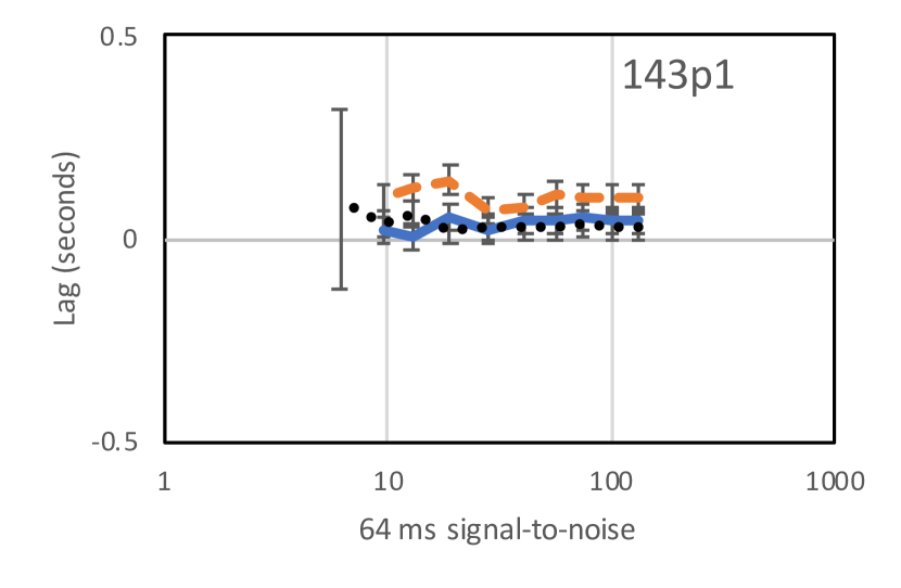
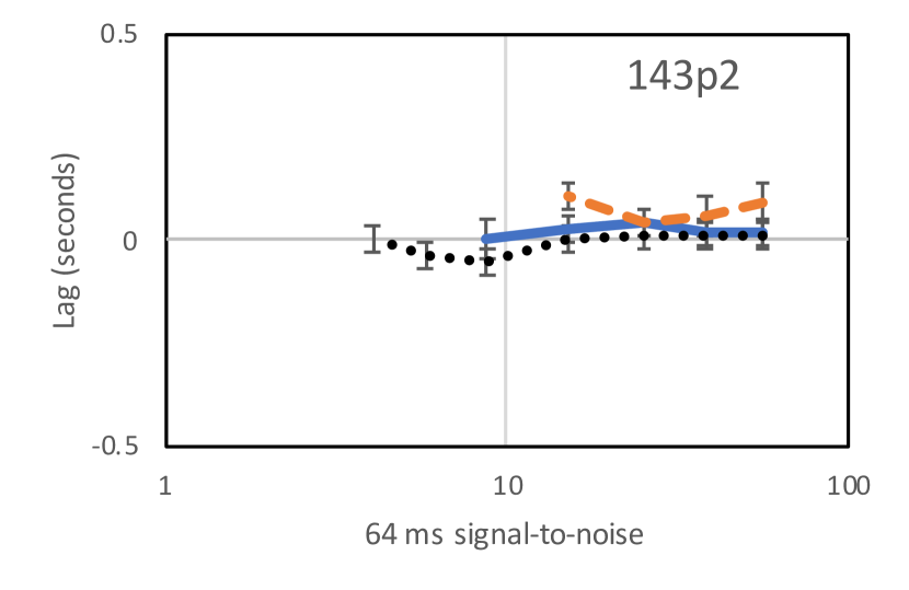
Figure 11: Data lags of pulses 143p1 (left panel) and 143p2 (right panel). Black dotted lines indicate lags between BATSE channels 3 and 2, blue solid lines indicate lags between BATSE channels 3 and 1, and orange dashed lines indicate lags between BATSE channels 4 and 1. Lags in both 143p1 and 143p2 decrease systematically with decreasing $S/N$.

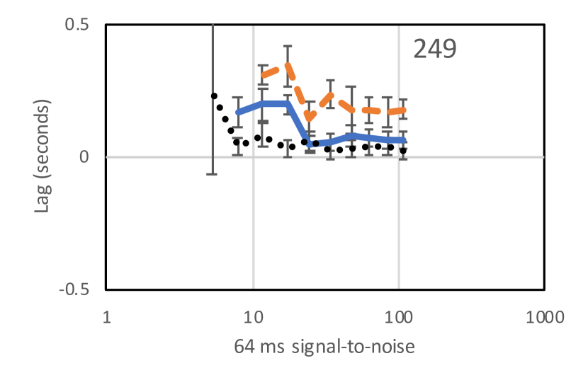
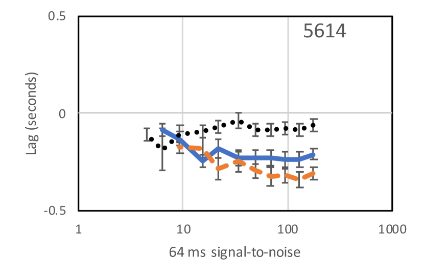
Figure 12: Data lags of pulses 249 (left panel) and 5614 (right panel). Black dotted lines indicate lags between BATSE channels 3 and 2, blue solid lines indicate lags between BATSE channels 3 and 1, and orange dashed lines indicate lags between BATSE channels 4 and 1. Lags in 249 remain constant with decreasing $S/N$ while those of 5614 increase systematically with decreasing $S/N$.

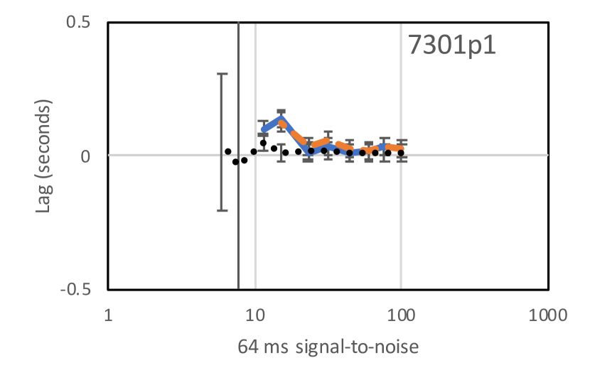
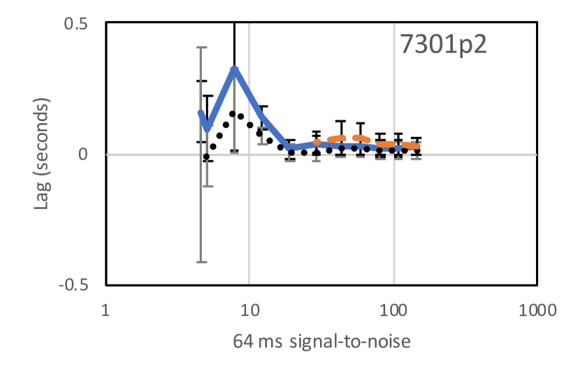
Figure 13: Data lags of pulses 7301p1 (left panel) and 7301p2 (right panel). Black dotted lines indicate lags between BATSE channels 3 and 2, blue solid lines indicate lags between BATSE channels 3 and 1, and orange dashed lines indicate lags between BATSE channels 4 and 1. Lags in 7301p1 do not undergo systematic changes, while lags in 7301p2 increase systematically by large amounts with decreasing $S/N$.

Pulse lag and duration are both luminosity indicators (Hakkila et al., 2008), yet neither seems to be systematically affected by decreased $S/N$, although lag results can be marginally affected when one lag channel is significantly noisier than the other. Thus, measurements of these characteristics at low $S/N$ are generally reliable, with uncertainties mostly produced by small number photon counting statistics.

3.2 Mirrors: Temporally Reflected Residuals

Because instrumental noise has been shown to smear out GRB pulse structure, we are forced to confront the fact that our best chance to learn about GRB pulse structure is to study the spectro-temporal evolutionary properties of bright, complex GRBs. The study of complex GRB pulse characteristics has generally been avoided primarily because authors have disagreed on the number of pulses represented in bursts containing structure if the structure cannot be attributed to noise. However, as a result of our analysis in Section 3.1.1, we are able to approach each bright episode under the assumption that it represents a single structured pulse.

The six pulses in our sample suggest that bright pulse residuals exhibit a wavelike function similar to that described by the residual model, but with a larger number of complete waves than the three used to develop Equation 7. The complex residual structures of these pulses can be seen in the left panels of Figures 1 $-$ 6. Hakkila & Preece (2014) assumed that the wave used in the empirical fitting function did not extend outside the Bessel function’s third zeros at $J_{0}(x=\pm 8.654)$ because the low- to moderate-$S/N$ pulse residuals showed no evidence of this. That assumption is not true at the higher $S/N$ values of pulses in this sample, where 143p1 appears to exhibit nine sets of up-and-down residual fluctuations, 143p2 has five, 249 has at least seven, 5614 has six, 7301p1 has roughly six, and 7391p2 has three. However, since the residual function successfully characterized these structures at lower $S/N$, we suspect that the high-$S/N$ structures are extensions of this phenomenon, and that they have similar origins even though each pulse shows structures that occur on different timescales with differing amplitudes.

We have unsuccessfully attempted to extend the residual model to these pulses beyond the Bessel function’s third zeros. The additional wave features present at high $S/N$ cannot be adequately fitted by simply extending the Bessel function limits and changing the $t_{0}$, $a$, $\Omega$, and $s$ values. The function incorrectly models these additional waves because the residual model was fine-tuned to work with moderate $S/N$ GRB pulse structures; it cannot be extrapolated to the unexpected structures we encounter at high $S/N$.

The wavelike structures at the beginning of each pulse are observed to have similar characteristics to those at the end of the pulse, except that they appear to be temporally inverted. The residual function described in Equation 7 partially explains this, as it was developed with an implicit recognition that GRB pulse residuals were best fit by temporally-inverted structures. The reason why this model worked was not understood. However, closer examination shows that the many maxima and minima of the pulse residual structures occur in a temporally-mirrored order, with near-reversible shapes. The structures at the beginning of each pulse are decent reversed facsimiles of the structures at the end of the pulse. Furthermore, the wavelike features at the beginning of pulses are compressed relative to those at the ends of pulses, apparently coordinated with the pulse’s asymmetry. When an odd number of waves is found, this indicates that the time of reflection occurs near a wave maximum. When an even number of waves is found, this indicates that the time of reflection lies at a wave minimum.

Since the residual function is an incomplete representation of the residual structure, we choose to more accurately characterize the mirrored residual structure in our sample. We do this by folding the residuals over at a pulse’s temporal symmetry point (the time of reflection, which we call $t_{\rm 0;mirror}$), then stretching the folded reversed residuals by an amount $s_{\rm mirror}$ until the folded wave prior to the reflection time (generally on the rising part of the pulse light curve) matches the wave following the reflection time (generally on the decaying part of the light curve). We find these values iteratively, by cycling $t_{\rm 0;mirror}$ through a range of possible values, folding and reversing the residuals at each possible time of reflection, then cycling $s_{\rm mirror}$ through a range of possible values so as to stretch the reversed-residuals to match the forward- and reversed stretched residual light curves. The CCF calculated at each step is used to compare the quality of the matches, with the optimal CCF value identifying the best characterization of $t_{\rm 0;mirror}$ and $s_{\rm mirror}$. We note that $t_{\rm 0;mirror}$ is similar to $t_{0}$ (defined in Equation 7) except that $t_{\rm 0;mirror}$ is no longer necessarily measured from the time when the residual function is a maximum ($t_{0}$ is), and that $s_{\rm mirror}$ is similar to $s$ except that it is measured from $t_{\rm 0;mirror}$ rather than from $t_{0}$. Our folding and stretching approach also uses all residuals rather than just those fitted by Equation 7. In other words, $t_{\rm 0;mirror}$ and $s_{\rm mirror}$ are less model-dependent definitions than $t_{0}$ and $s$, since the former require only a pulse fit to be made prior to their measurement whereas the latter require both a pulse fit and a residual fit.

The results of mirroring and stretching the residuals of our six pulses are shown in Figures 14 $-$ 16. The times given in these figures are referenced to $t_{\rm 0;mirror}$ (seventh column of Table 2) rather than to the trigger time ($t=0$ seconds), and these times only describe the decay portion of the residuals (dotted line), because the rise times (solid line) have been time-inverted and stretched. Despite the bright, non-randomly distributed residual structures, the fits are good. The optimum values of the CCF exceed $0.6$ for these residuals, indicating a strong correlation between the structures preceding the time of reflection and those following it. The CCFs of three of the pulses (143p2, 5614, and 7301p2) exceed 0.8. We note that the fit we chose for 143p1, with a CCF of 0.60, was slightly worse than the optimal fit of 0.64 $-$ we chose this fit because it pairs all but one of the residual peaks whereas the optimal fit misses three peaks in order to pair the two deepest troughs.

The fitted characteristics of the mirrored residual parameters $s_{\rm mirror}$ and $t_{\rm 0;mirror}$ are compared to their counterparts $s$ and $t_{0}$ in Table 2. The pulse asymmetry $\kappa$ is included for comparison with the $s$ value for each pulse, as these parameters have previously been shown to anti-correlate; this anti-correlation is only loosely observed from these six pulses. Also indicated are the best-fit CCF values used to obtain the time-reversible characteristics. The values are generally in good agreement, and differ primarily for the reasons described above.

We estimate the significance of the mirroring by comparing the time-inverted, stretched residuals preceding the time of reflection to those following it. We use the $p-$values obtained from a Spearman Rank-Order test to compare the two distributions, after first interpolating the time-reversed and stretched residuals so that they contain the same number of data points as the better-sampled post-$t_{\rm 0;mirror}$ residuals. This approach gives us a likelihood that the residuals are related, without providing information about how closely the intensities match one another. The $p-$ values found for all pulses are significant ($p<10^{-8}$), indicating that residuals following $t_{\rm 0;mirror}$ are time-reversed and stretched versions of those preceding it.

To ensure that our fitting procedure has not inadvertently biased the results, we repeat the analysis after excluding all intensities less than $3\sigma$ away from the mean background rate (this data truncation eliminates any temporal correlations that might result from incompletely-fitted monotonic pulse components and/or backgrounds). We define $p-$bright to be the Spearman Rank-Order correlation $p-$value obtained from comparing these truncated data. The results of the Spearman Rank-Order test are shown in the final column of Table 2; all six pulses have $p-$bright $<10^{-4}$. The strongest matches are found for 7301p2, 249, and 143p2 (small $p-$bright values indicate support for the stretched temporal inversion hypothesis). The least significant match is found for 5614 due to the small number of bright data points this pulse contains. We conclude that the time-reversed and stretched residuals are not an artifact of our data analysis procedure. Furthermore, we will show in Section 4 that the increased significance of $p-$ relative to $p-$bright, when coupled with hardness evolution, indicates additional evidence for faint time-reversed and stretched structures extending farther from the time of reflection as opposed to inadequate monotonic pulse-fitting.

We note that half the measured $t_{\rm 0;mirror}$ values (143p1, 5614, and 7301p1) occur at times where the residuals are at a minimum rather than at a maximum. Since $t_{0}$ by definition measures reflection from a maximum value of the residuals, $t_{\rm 0;mirror}$ and $t_{0}$ can differ significantly (see Table 2), as can $s$ and $s_{\rm mirror}$. This result demonstrates that Equation 7 is not an accurate characterization of complex residual structures. It also explains why some pulse duration ($w$) and asymmetry ($\kappa$) measurements shown in Figure 10 undergo discontinuous changes as $S/N$ is reduced: residual fit parameters change as structure is incrementally washed out by noise.

Figure 14: The mirrored and stretched residuals of BATSE triggers 143p1 and 143p2 (after removing the Norris et al. (2005) fit). The cross-correlation function yields values of 0.60 (143p1) and 0.84 (143p2) when the residuals from the pulse rise (solid line) are inverted, stretched, and overlaid with the residuals from the decay side (dotted line).

Figure 15: The mirrored and stretched residuals of BATSE triggers 249 and 5614 (after removing the Norris et al. (2005) fit). The cross-correlation function yields values of 0.72 (249) and 0.81 (5614) when the residuals from the pulse rise (solid line) are inverted, stretched, and overlaid with the residuals from the decay side (dotted line).

Figure 16: The mirrored and stretched residuals of BATSE triggers 7301p1 and 7301p2 (after removing the Norris et al. (2005) fit). The cross-correlation function yields values of 0.66 (7301p1) and 0.81 (7301p2) when the residuals from the pulse rise (solid line) are inverted, stretched, and overlaid with the residuals from the decay side (dotted line).

Table 2: Fitted Pulse vs. Time-Reversible Residual Properties

Pulse	$\kappa$	CCF	$s$	$s_{\rm mirror}$	$t_{0}$	$t_{\rm 0;mirror}$	$p-$bright
143p1	$0.75\pm 0.01$	$0.60$	$0.45\pm 0.04$	$0.67$	$4.07\pm 0.05$	$3.15$	$2\times 10^{-6}$
143p2	$0.59\pm 0.02$	$0.84$	$0.50\pm 0.01$	$0.51$	$48.09\pm 0.01$	$48.03$	$2\times 10^{-14}$
249	$0.07\pm 0.02$	$0.72$	$0.56\pm 0.02$	$0.74$	$21.51\pm 0.03$	$21.70$	$3\times 10^{-22}$
5614	$0.69\pm 0.01$	$0.81$	$0.19\pm 0.02$	$0.31$	$8.30\pm 0.01$	$8.92$	$2\times 10^{-4}$
7301p1	$0.51\pm 0.08$	$0.66$	$0.82\pm 0.06$	$0.96$	$16.62\pm 0.03$	$17.8$	$2\times 10^{-7}$
7301p2	$0.52\pm 0.02$	$0.81$	$0.48\pm 0.02$	$0.72$	$165.40\pm 0.07$	$165.60$	$3\times 10^{-45}$

4 Discussion

GRB pulse temporal and spectral behaviors are closely linked, with pulse structure playing an important role in characterizing spectral evolutionary behavior. Pulse spectro-evolution is often characterized in terms of “hard-to-soft” and “intensity tracking” behaviors (e.g., Wheaton et al. (1973); Golenetskii et al. (1983); Norris et al. (1986); Paciesas et al. (1992)); these terms unfortunately suggest two distinct and bimodal characterizations when in fact a large continuous range of behaviors exists (e.g., Kargatis et al. (1994); Bhat et al. (1994); Ford et al. (1995)). We shall demonstrate that much of this variation may not be real, but may instead result from the lack of a consistently-applied pulse definition. We have previously demonstrated that essentially all pulses undergo hard-to-soft spectral evolution in that they are harder at the pulse onset than they are late in the decay phase (Hakkila et al., 2015, 2018). Despite this gradual softening, spectral re-hardening of moderately bright GRB pulses typically occurs around the times that pulse structure occurs, as found from the three residual peaks. Spectral evolution is therefore subject to the relative hardnesses of the residual peaks. Pulses appear to evolve “hard-to-soft” if their central peaks are softer than their precursor peaks, whereas they follow “intensity tracking” behaviors if their central peaks are harder than their precursor peaks. Depending on the relative hardnesses of the peaks, there exist a wide range of intermediary behaviors (Hakkila et al., 2015) that authors often either exclude from their analyses or force-classify into either the “intensity tracking” or “hard-to-soft” categories.

Asymmetry also plays a role in pulse hardness evolution: asymmetric pulses are harder overall and have pronounced hard-to-soft evolution; these contrast with symmetric pulses that are softer and have weak hard-to-soft evolution Hakkila et al. (2015). This weak evolution can result in softer precursor peaks than central peaks, producing intensity tracking behaviors.

Using BATSE’s four energy channels, we define a counts hardness ($hr$) in each time bin $i$ as:

$$hr_{i}=\frac{C_{3i}+C_{4i}}{C_{1i}+C_{2i}}$$ (14)

where $C_{1i},C_{2i},C_{3i}$, and $C_{4i}$ are the counts/bin in channels 1 ($20-50$ keV), 2 ($50-100$ keV), 3 ($100-300$ keV), and 4 (300 keV $-1$ MeV), respectively. This counts hardness has been chosen instead of a standard ratio like $hr_{32}=C_{3}/C_{2}$ in order to increase the number of photon counts in each bin, making the hardness more reliable for use on short timescales and thus in probing spectral evolution.

The pulse hardness evolution of moderately bright BATSE pulses (64 ms resolution), Swift pulses (64 ms resolution), and short BATSE pulses (4 ms resolution) have been studied previously in aggregate samples of pulses (Hakkila et al., 2015, 2018). The technique used was to combine the energy-dependent light curves of many pulses by 1) scaling the durations of the pulse sample to the unitless fiducial timescale, 2) subtracting out the monotonic pulse model of each pulse to obtain residuals, 3) aligning the residuals to the zeros, minima, and maxima of the residual function to account for asymmetry, 4) summing the energy-dependent residual counts from different pulses to obtain composite time-dependent counts in each energy channel, and 5) using these composite counts to obtain time-dependent hardnesses to describe aggregate pulse evolutionary behavior. The fiducial time interval used in these analyses (Equation 4) had the additional benefit of recognizing that residual structures often begin before and end after the monotonic pulse component does.

The six pulses used in this analysis are bright enough that the counts hardness evolution of each can be studied individually, rather than in aggregate. However, the fiducial timescale no longer completely encapsulates the structured components of all sampled pulses because some of the complex residual wave structures extend beyond the three known residual peaks, and therefore beyond the boundaries of the fiducial timescale. It thus makes more sense to bound each pulse’s hardness evolution by its mirrored residual timespan rather than by its fiducial timescale.

4.1 BATSE Trigger 143

Both of BATSE trigger 143’s asymmetric pulses exhibit hard-to-soft spectral evolution. However, 143p1 is characterized by a complex residual structure whereas 143p2 is triple-peaked; the added structure in 143p1’s light curve causes it to undergo more frequent hardness fluctuations.

Pulse 143p1’s rapid intensity variations are accompanied by spectral re-hardening (Figure 17, left panel); these are difficult to temporally resolve given the small numbers of counts available per bin during the short variable intervals. We demonstrate these variations using a combination of the hardness evolution plot (Figure 17, left panel), the fitted pulse and residual light curves (Figure 1), and the time-reversible and stretched structures (Figure 14; left panel).

Links between the triple-peaked pulse structure and hardness evolution are shown using the approach of Hakkila et al. (2015, 2018). Figure 17 (left panel) shows the hardness evolution relative to the times of the precursor peak (downward-facing red arrow), the valley between the precursor and central peaks (upward-facing red arrow), the central peak (downward-facing black arrow), the valley between the central and decay peaks (upward-facing blue arrow), and the decay peak (downward-facing blue arrow). The precursor peak and the decay peak provide rough estimates of the fiducial timescale, and therefore of the monotonic pulse duration.

Pulse 143p1 is odd in that the peak of the monotonic pulse ($\tau_{\rm peak}=1.7$ seconds) does not align well with the peak of the residuals ($t_{0}=4.1$ seconds; see Table 2). The central residuals peak of 143p1 roughly aligns with a series of fluctuations occurring on the downslope of the light curve. The time of reflection found from the time-reversed and stretched residuals is identified in Figure 17 (left panel) by a vertical dotted line.

The three peaks of the residual function are smoothed representations of a more complex residual structure that can be seen by comparing 143 p1’s hardness evolution to both the fitted residual structure (Figure 1, left panel) and the time-reversible residual structure (Figure 14; left panel). The time of reflection at $t_{\rm 0;mirror}=3.15$ takes place almost a full second before the fitted residual peak; this corresponds to a deep residual valley (left panel of Figure 14). The pulse undergoes hardening immediately prior to and following $t_{\rm 0;mirror}$; this hardness bump encompasses a set of unresolved peaks occurring at around $t=2$ seconds that are mirrored with three closely-spaced peaks occurring around $t=6$ seconds. These mirrored structures are seen in the left panel of Figure 14 occurring between 1 and 2 seconds after the time of reflection. Two bright peaks at $t=1$ and $t=6$ seconds are also mirrored, as is the hard bump at the trigger ($t=0$ seconds) with two peaks at $t=8$ and $t=9$ seconds. The spectrally hardest part of the pulse occurs at this trigger bump. The bump shows up on the time-reversed light curve (Figure 14; left panel) roughly 4 seconds after $t_{\rm 0;mirror}$, where it coincides with two spikes at $t=8$ and $t=9$ seconds (Figure 1; left panel).

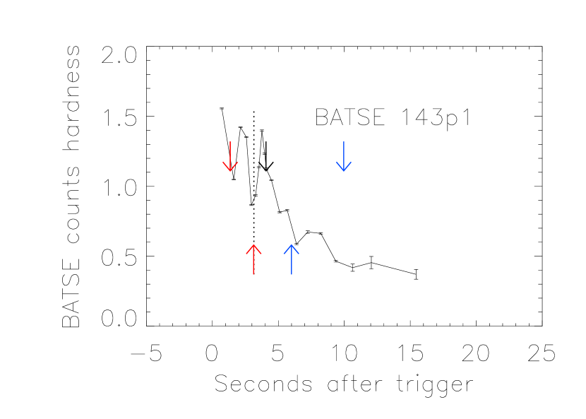
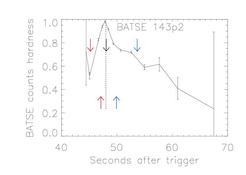
Figure 17: Counts hardness ($hr$) evolution of BATSE pulses 143p1 (left panel) and 143p2 (right panel). In this and subsequent figures, downward facing arrows indicate the approximate times of the precursor peak (red), central peak (black), and decay peak (blue). Upward facing arrows indicate the time of the valley separating the precursor peak (red) and decay peak (blue) from the central peak.

The residuals of 143p2 exhibit three sharp peaks (Figure 2) that align well with the residual function; these are the precursor peak at 45 seconds, the central peak at 48 seconds, and the decay peak at 52 seconds. Two other faint bumps (at 43 seconds and 59 seconds) are also visible beyond the fiducial time interval. The stretched and mirrored residuals (right panel of Figure 14) are centered at $t_{\rm 0;mirror}=48.03$ seconds, which coincides with the position of the central peak (identified by the dotted vertical line in the right panel of Figure 17). The precursor and decay peaks are found 4 seconds after $t_{\rm 0;mirror}$, and the two bumps can be seen about 12 seconds after $t_{\rm 0;mirror}$. Pulse 143p2 is softer and undergoes more gradual hard-to-soft evolution than 143p1 (right panel of Figure 17), re-hardening at each peak and bump, and demonstrating that the bumps represent faint pulse components.

4.2 BATSE Trigger 249

BATSE trigger 249 exhibits multiple residual peaks (Figure 3) that build in intensity from the trigger to the central peak and lessen thereafter. The residual model places the precursor peak at 17 seconds, the central peak at 22 seconds, and the decay peak at 27 seconds. However, two other sets of paired peaks are also present (the first pair at 10 seconds and 42 seconds, and the second pair at 15 seconds and 32 seconds). The central peak aligns closely with $t_{\rm 0;mirror}$, and the pairing of the various sets of peaks can be seen in the left panel of Figure 15.

Trigger 249 demonstrates the inadequacy of characterizing a pulse’s duration based solely on monotonicity assumptions. The central monotonic part of the pulse, extending from roughly 15 to 28 seconds, contains most of the flux, but it is clear from mirrored residuals in Figure 15 and the hard-to-soft evolution in Figure 18 (left panel) that this pulse starts at the trigger and continues for roughly 50 seconds (see also Figure 3). The pulse evolves consistently from hard-to-soft over the timescale spanned by the mirrored residuals, while the central portion of the pulse undergoes a re-hardening at the precursor peak that is generally maintained until the end of the decay peak; this hardness plateau representing the monotonic part of the pulse (left panel of Figure 18) seems to stand apart from the pulse’s overall hardness evolution.

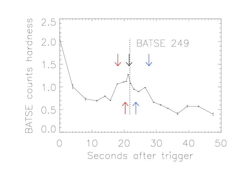
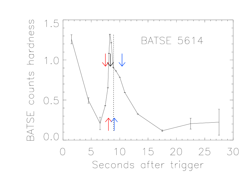
Figure 18: Counts hardness ($hr$) evolution of BATSE pulses 249 (left panel) and 5614 (right panel).

4.3 BATSE Trigger 5614

Trigger 5614’s smooth light curve (Figure 4) is nearly monotonic and has only low-amplitude residuals. These can almost be fitted by the triple-peaked residual model. However, the residual structure has too many lobes, and these (Figure 15, right panel) are consistent with stretched and mirrored structures similar to those found in the other pulses. The time of reflection for 5614 occurs at $t_{\rm 0;mirror}=8.92$ seconds. This occurs, similar to 143p1, at a minimum in the residuals, indicating that a pulse’s peak intensity is not always augmented by the peak intensity of the residuals. The pulse has two distinct sets of mirrored and stretched residuals: the central peak located at $t=8.3$ seconds correlates with a three-peaked structure at $t=10.5$ seconds (this is the first peak found 1.5 seconds after the time of reflection in Figure 15, right panel), and a peak at $t=7.8$ seconds matches a bump at $t=13$ seconds (this is the second peak found 4 seconds after the time of reflection in Figure 15, right panel). As in the case of 249, 5614 undergoes significant re-hardening at the time of the precursor peak and maintains this throughout the central and decay peaks (right panel of Figure 18). In fact, the hardening is so pronounced that the pulse appears to follow intensity-tracking behavior rather than the expected hard-to-soft evolution. Supportive evidence for this interpretation comes from the pulse’s spectral lags, which are negative. GRB pulses canonically evolve from hard-to-soft, with the amount of evolution primarily guided by a pulse’s overall hardness and asymmetry. How can we reconcile the apparent existence of an intensity tracking pulse with our interpretation of a hard-to-soft evolution? How can we interpret negative spectral lags in terms of hard-to-soft evolution? The answers to these questions lie in information supplied by 5614’s mirrored residual function.

Equation 7 only partially captures 5614’s pulse structure. This can be seen in the pulse and residual light curves (Figure 4), and it is also indicated by the seven-second delay between the trigger time and the rise of the monotonic pulse intensity. The episode that triggers 5614 is clearly part of the burst, and the presence of extended time-reversed and stretched residuals leads us to believe that this low intensity triggering bump must also be part of the pulse. When we extend the pulse hardness evolution to include this episode we find that it is spectrally very hard. With the addition of this early peak, the pulse evolves hard-to-soft as expected instead of following its apparent intensity tracking behavior. Furthermore, Figure 18 (right panel) shows weak evidence of an extended mirrored tail at about $t=25$ seconds. Although the other residuals clearly match up in the mirrored residuals plot (Figure 15, right panel), the faint trigger bump around 25 seconds after $t_{\rm 0;mirror}$ is only barely visible.

The pulse undergoes a significant re-hardening at the time of the fitted precursor peak which it roughly maintains throughout the pulse’s central and decay peaks. This is similar to what is observed in pulses 143p2 and 249. However, the precursor peak of 5614 is not as hard as the central peak. Even more interesting, the precursor peak is brighter in channel 1 (20 - 50 keV) than the central peak is in channel 3 (100 - 300 keV), which can be seen in Figure 19. As a result of this peculiarity, the spectral lag calculated between channels 3 and 1 is negative, even though the pulse still undergoes hard-to-soft evolution with re-hardening at each of the peaks. In other words, the negative lag is an artifact created when the CCF mistakenly correlates the enhanced soft emission of the precursor peak for the pulse’s central peak intensity to find a lag. This type of spectro-evolutionary behavior, coupled as it is with GRB pulse residual structure, may explain the existence of many negative GRB spectral pulse lags.

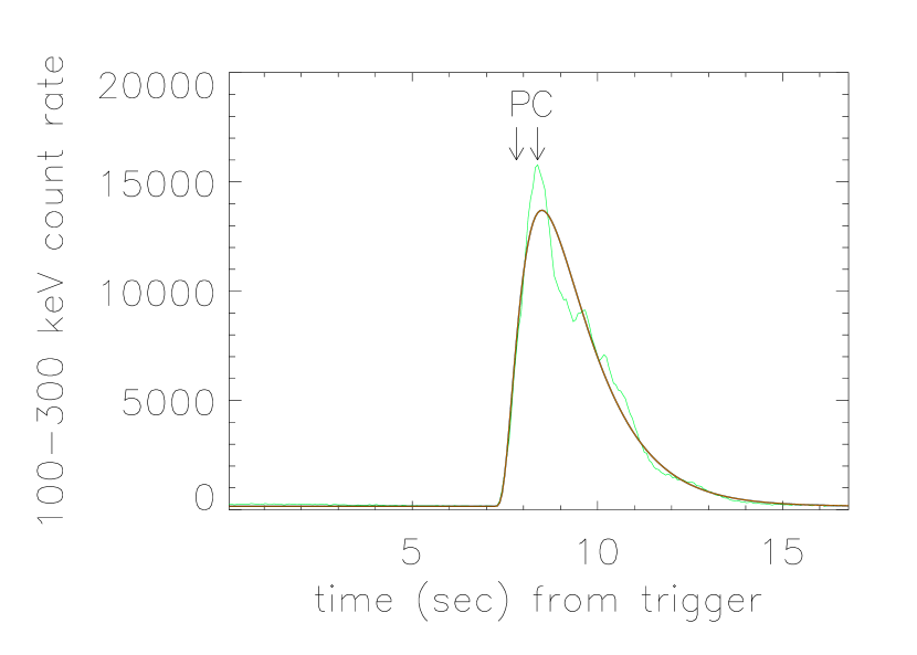
Figure 19: Pulse structure of 5614 in channel 3 (100 - 300 keV; left panel) and in channel 1 (20 - 50 keV; right panel). Arrows indicate the times of the brightest channel 1 emission (P, corresponding closely with the time of the precursor peak found from the residuals) and brightest channel 3 emission (C, corresponding closely with the time of the central peak found from the residuals). The precursor peak has a smaller channel 3/channel 1 counts ratio than the central peak, indicating that it is the softer of the two peaks. The precursor peak’s unexpected brightness causes the cross-correlation function to measure a negative lag when it aligns the brightest channel 1 emission with the brightest channel 3 emission, even though the right panel of Figure 18 shows that 5614 evolves from hard-to-soft.

4.4 BATSE Trigger 7301

BATSE 7301’s behavior is complex, even when compared to the other complex bursts being analyzed here. The complete light curve of 7301 is shown in Figure 20. In addition to 7301p1 and 7301p2, the burst contains two faint emission episodes starting $t=0$ seconds and at $t=32$ seconds, low intensity bumps at around $t=100$ seconds and $t=135$ seconds, and a long emission tail following 7301p2. This emission complicates simple explanations of 7301’s spectro-temporal evolution.

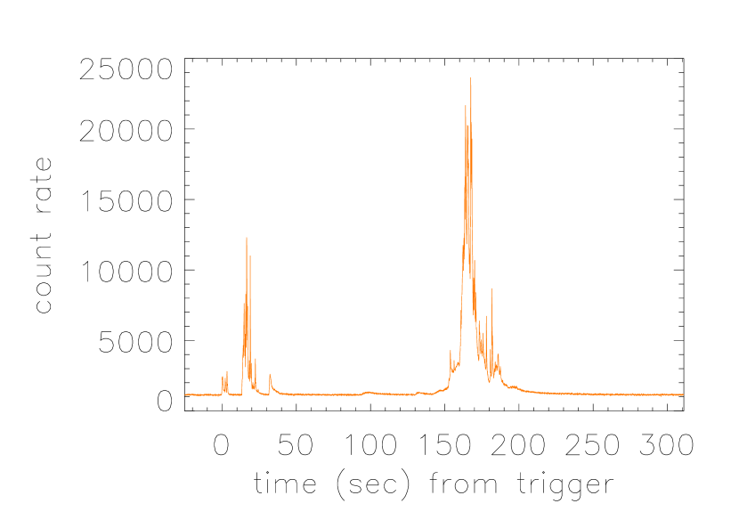
Figure 20: Full light curve of 7301.

The duration of 7301p1 depends on whether or not the pulse encompasses two faint emission episodes at $t=0$ seconds (the three-peaked ‘comb’) and $t=32$ seconds (the ‘shoe’). The optimum CCF value of 0.66 occurs for the mirrored residuals if these two faint emission episodes are treated as part of the 7301p1 pulse structure (shown in Figure 16). This inclusion improves the CCF, which would be 0.58 otherwise. The value of $s$ measured from the mirrored residuals is $s_{\rm mirror;with}=0.99$ (essentially unstretched) compared to $s_{\rm mirror;without}=0.72$ when the comb and the shoe have been excluded. Each of these measures are in moderate agreement with the value of $s=0.82$ measured from the residual function.

We favor the hypothesis that the comb and the shoe belong to 7301p1. If they do, then the two brightest peaks in the main pulse (at $t=16.6$ seconds and $t=19$ seconds in Figure 5 and occurring 1.2 seconds after $t_{\rm 0;mirror}$ in Figure 16, left panel) are found to align, as do the two valleys immediately preceding and following them (the deep valley at $t=15.5$ seconds and the shallower valley at $t=20.5$ seconds seen in the left panel of Figure 5); these valleys can also be seen 3 seconds after $t_{\rm 0;mirror}$ in the left panel of Figure 16. Furthermore, it is no longer disturbing that this alignment causes $t_{\rm 0;mirror}$ to occur at a residual function minimum rather than at a maximum, since similar behavior was found in 143p1 and 5614. Finally, although the hardness evolution (shown in the left panel of Figure 21) is consistent with the hard-to-soft spectral evolution of three separate pulses, it is also consistent with the gradual hard-to-soft evolution of a single pulse that re-hardens at each emission peak. Occam’s Razor leads us to think that these behaviors represent a single pulse rather than multiple pulses.

BATSE pulse 7301p2 exhibits very strong evidence of temporally-mirrored and stretched residuals. The time of reflection ($t_{\rm 0;mirror}=165.6$ seconds) occurs at a narrow residual peak which is closely bounded by a pair of mirrored and stretched peaks at $t=163$ seconds and $t=167$ seconds (seen 2 seconds after $t_{\rm 0;mirror}$ in the right panel of Figure 16), and by another broader pair of peaks at $t=153$ seconds and $t=186$ seconds (16 seconds after $t_{\rm 0;mirror}$). Additionally, the faint emission at $t=100$ seconds aligns with the long 7301p2 pulse tail extending out past $t=200$ seconds; this can be observed from 20 to 50 seconds after $t_{\rm 0;mirror}$.

The hardness evolution of 7301p2 is similar to what is observed in pulses 249, 5614, and 7301p1. This behavior is characterized by weak hard-to-soft spectral evolution punctuated by sustained hard emission during the central ‘monotonic’ pulse. Spectral re-hardening occurs at each intensity peak. Of all the pulses studied in this sample, 7301p2 has the most gradual hard-to-soft evolution, and is thus most comparable to an intensity-tracking pulse.

Occam’s Razor leads us to believe that BATSE 7301 contains only two distinct pulses characterized by large and rapid intensity fluctuations. The durations of these two pulses, as measured from their stretched and mirrored residuals, span over 250 seconds. This interpretation is considerably different than what would be made by assuming that a pulse constitutes any emission spike not attributed to instrumental noise.

Incorporating the comb and shoe features into 7301p1 increases the pulse’s duration and makes it similar to that of 7301p2. Pulses 143p1 and 143p2 also have similar durations. Although it is hard to draw conclusions about relative pulse durations from only two GRBs, we note that this suspected relationship might warrant further study if other bright, structured, multi-pulsed GRBs can be found and analyzed.

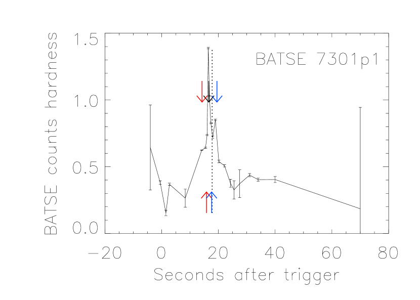
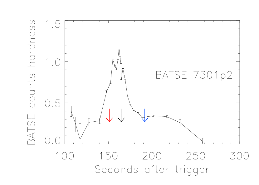
Figure 21: Counts hardness ($hr$) evolution of BATSE pulses 7301p1 (left panel) and 7301p2 (right panel).

4.5 Are these Pulse Characteristics Ubiquitous?

The six bright GRB pulses analyzed here exhibit measurable spectro-temporal features that are not likely to have been washed out by instrumental effects. If these properties are representative of properties that would be found in fainter pulses, then these are probably defining GRB pulse characteristics that can be used to constrain GRB physics. These characteristics suggest that GRB pulses exhibit smooth monotonic components that evolve from hard-to-soft and structured components that undergo time-reversed and stretched variations. Monotonic component asymmetry occurs in tandem with compression and stretching of the time-reversible structured component.

We do not know if the time-reversed and stretched residuals found here apply to all GRB pulses. The greatest difficulty in ascertaining how generic these characteristics are relates to our inability to thoroughly characterize GRBs at low $S/N$. At low $S/N$ it is difficult to delineate complex single-pulsed GRBs from multi-pulsed ones, and measurement of the characteristics that might otherwise prove helpful are buried in statistical uncertainties. We also note that many faint GRBs have different properties than those found in bright GRBs. For example, Norris et al. (2000) show that some faint GRBs have long CCF data lags and soft spectra, but they also show that there are no bright versions of these bursts. Our analysis suggests that these characteristics cannot be created simply by observing a bright, hard, short-lag burst at lower $S/N$.

We have performed a cursory exploration of a few complex BATSE GRB pulses, and have found more of these types of events. For example, again using the cross-correlation function to describe fit quality, we find that triggers 1008 ($S/N=22.0$, $CCF=0.64$), 1114 ($S/N=29.2$, $CCF=0.54$), 3954 ($S/N=32.4$, $CCF=0.50$), 5417 ($S/N=39.0$, $CCF=0.40$), and 6422 ($S/N=36.5$, $CCF=0.43$) all show evidence of time-reversible and stretched structures even though they are observed at lower $S/N$ than the six pulses in our sample. That pulses with these $S/N$ values show complex and possibly time-reversible and stretched structure is consistent with the results shown in Figure 9; if time-reversed and stretched residuals are characteristic of all GRB pulses, then as many as 100 BATSE GRBs should have been observed at large enough $S/N$ to exhibit these characteristics.

Hakkila et al. (2018) have recently used 4-ms resolution BATSE TTE (time-tagged event) data to demonstrate that short GRBs also exhibit pulse structure consistent with this paradigm. Roughly 40 GRB pulses in the TTE Pulse Catalog have complex structures that might exhibit time-reversed and stretched residuals. However, few of these pulses have $S/N>15$. The $S/N$ of these pulses can be increased by using coarser time binning (say, 64 ms). However, using coarser temporal binning also washes out pulse structure by decreasing temporal resolution (see also Burgess (2014)).

Time-reversible and stretched residual structures are likely to be measurable in GRB pulses observed by other satellite experiments, such as Swift and Fermi’s GBM experiment. Swift and GBM have better temporal resolution than BATSE. However, Swift operates at lower energies where the sky is noisier, and GBM has a smaller surface area than BATSE. Both of these characteristics reduce $S/N$. A preliminary analysis of Swift GRBs has yielded few with complex structures among hundreds with simple structures. However, simple single-pulsed GRBs were favored in the selection of that sample, so work on Swift data is ongoing. We have begun studying GBM data in conjunction with members of the GBM team; we do not yet have estimates of how many GRB pulses might exhibit time-reversible and stretched residual structures, but we are encouraged by GBM’s low systematic noise.

Some GRBs characterized by overlapping emission episodes are found to contain distinguishable yet overlapping pulses. Knowledge of the residual function can help us in these cases. As an example we show fits for BATSE trigger 148 (Figure 22). This burst can be successfully fitted by two overlapping pulses; 148p1 is a blended pulse with $S/N=17.1$ while 148p2 is a blended pulse with $S/N=12.9$. We note that this technique only works for a small subset of overlapping BATSE GRBs that are bright with bright residual structures, and thus cannot generally help resolve confusion over the number of pulses in a faint GRB.

5 Smoke and Mirrors: Defining GRB Pulses

“Smoke and Mirrors” refers to the obscuration of a truth using misleading or irrelevant information. Our own study has inadvertently obscured the truth by stating that GRB pulse durations are not affected by $S/N$. Although we demonstrated that fitted pulse durations can be accurately recovered over a range of $S/N$, we subsequently showed that these monotonic components often have shorter durations than their associated residual structures. Unlike the monotonic pulse components, these faint residual structures can disappear into the background at low- to moderate-$S/N$ when monotonic pulse components do not. Furthermore, faint residual “bumps” observed in some GRBs can be misinterpreted as being separate monotonic pulses. Treating these structures as separate pulses misleads us to think that pulses are shorter, more common, and more widely separated than they actually are.

Should time-reversed and stretched residuals be used to redefine GRB pulses? Revising the pulse definition would certainly be an improvement over the current situation, where investigators explain GRB physics in terms of a wide range of different and often incompatible pulse definitions. This incongruity makes it nearly impossible to tell whether or not two models are consistent with one another, or even if they are both consistent with the data. We suspect that it is too early to ask the GRB community to accept a new pulse definition. First of all, such a definition would only be viable when applied to bright (high $S/N$) bursts; bursts of intermediate intensity only exhibit the triple-peaked residual structure while faint bursts have the appearance of monotonic bumps. Second, the definition might be instrument-dependent; more work needs to be done to clarify selection biases introduced by satellites with different sensitivities working in different energy ranges. Third, accepting a new definition prematurely might prevent us from recognizing variations of this behavior or perhaps other behaviors belonging to different classes of objects. Without formally recommending a new GRB pulse definition, we ask that other researchers be aware of the non-monotonic nature of most GRB pulses, and of the pulse characteristics generally associated with non-monotonicity, so that results of various analyses can be more readily compared.

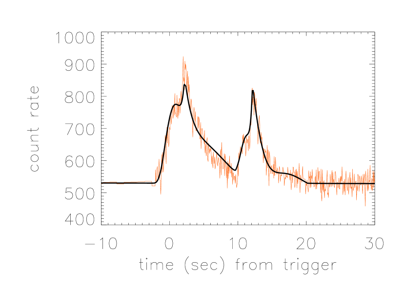
Figure 22: Fitted light curve of BATSE trigger 148, showing the delineation of two overlapping pulses.

6 Interpretation

6.1 Physical Explanations for the Time-Reversed Residual Structures

Despite the results of our analysis, we find it hard to imagine a physical mechanism capable of producing structured, time-reversible, stretched residuals. Since we think it is unlikely that the temporal mirroring and stretching found in GRB pulse structure is due to a time-reversed process, we suspect that it must instead indicate a kinematic process.

Natural objects rarely exhibit time-symmetric light curves, but kinematic mechanisms explain the ones that do. Simple time-reversed light curves are produced by gravitational microlensing when a distant source passes behind a compact foreground object (Paczynski, 1986a). When the foreground object is a binary, microlensed light curves can exhibit any of a wide range of complex symmetric temporal structures (e.g., see Liebig et al. (2015)). Although we do not suspect that time-reversed and stretched GRB light curve structures are produced by gravitational microlensing, we note that the black holes formed during the GRB emission might be capable of providing the necessary environmental conditions.

We suspect that kinematic motions causing mirrored and stretched residuals are directly related to jets and the expansion accompanying GRB explosions. Furthermore, since the mirroring is often coupled to both pulse asymmetry and evolving spectral hardness, we suspect that it is an indicator of how and when energy is fed into a GRB system.

Current GRB models do not naturally explain the existence of time-reversed and stretched residuals. Although time-reversed properties and stretching went into the development of the Hakkila & Preece (2014) residual function, these characteristics have largely gone unmentioned in the literature other than by the authors, who attributed them to forward and reverse shocks. This interpretation now seems unlikely given that the residual features extend well beyond three simple peaks. To our knowledge no standard GRB model has specifically predicted the existence of time-reversed GRB pulse structures.

The mechanism by which GRB prompt emission is produced is still largely unknown. The standard model states that it originates from material ejected relativistically during stellar black hole formation (Rees & Meszaros, 1994). The rapid variability of GRB prompt emission indicates that it arises internally from within the expanding material (Sari & Piran, 1997). Following the recent Dai et al. (2017)) review, we list three general mechanisms by which GRBs might produce pulsed emission:

1. Synchrotron shocks (Meszaros et al., 1993; Tavani, 1995). Mildly relativistic shocks are thought to occur when faster jet ejecta catches up with slower ejecta (Rees & Meszaros, 1994; Kobayashi et al., 1997; Daigne & Mochkovitch, 1998); synchrotron shocks occur in optically thin regions and models predict smoothly-varying light curves for which pulse duration reflects variations in the intensity of the central engine (Kobayashi et al., 1997; Daigne & Mochkovitch, 1998; Panaitescu et al., 1999).

2. Photospheric emission (e.g., Paczynski (1986b); Goodman (1986); Pe’er (2008); Beloborodov (2011)). A quasi-thermal spectrum is produced when the ejecta becomes transparent to its own radiation; these spectra can be made non-thermal with the addition of a low-energy tail produced by synchrotron emission and a high-energy tail produced by comptonization (e.g., Thompson (1994); Rees & Mészáros (2005); Pe’er et al. (2006); Beloborodov (2010); Ryde et al. (2011)).

3. Magnetic reconnection. If magnetization is large and emission occurs in an optically thin region where shocks cannot develop, then accelerated electrons should be able to radiate nonthermal or quasi-thermal spectra (Spruit et al., 2001; Drenkhahn & Spruit, 2002; Giannios & Spruit, 2005; Zhang & Yan, 2011).

Very little is known about the detailed microphysics capable of producing emission in any of these models.

Pulse durations and separation times can provide valuable clues to understanding GRB kinematics. Among other things they can be used to determine whether the progenitor undergoes a long-lasting or an impulsive ejection process. The relative rarity of GRB pulses per burst, pulse durations as defined by residuals that extend beyond the monotonic component, the existence of time-reversed and stretched residuals, and hard-to-soft pulse spectral evolution all place surprising and potentially strict constraints on kinematic characteristics of GRB models.

Based on our findings, we propose four general kinematic models to demonstrate how these observations impose constraints. We recognize that not all kinematic models are compatible with the three variations of the standard model described above.

Model 1

Radiation is emitted when an impulsive impactor encounters obstructions in a medium along its path, followed by an abrupt course reversal that causes it to pass through the medium in reverse order. In agreement with the standard model, the impactor-cloud interactions must be mildly relativistic because both the obstructions and mirror must move toward the observer faster than the impactor.

Model 2

An impulsive impactor moves through a symmetrically-structured medium, causing radiation occurring at the beginning of the interaction to be in reverse order to that occurring at the end of the interaction. The structure on the central engine-facing side is probably compressed relative to the structure on the other side.

Model 3

Sustained radiation is produced as a symmetrically-structured impactor moves through a simple medium. Despite general structural symmetry, the impactor is probably compressed on its leading face as it moves away from the central engine.

Model 4

Waves are generated as material moves through a symmetrically-distributed non-uniform medium. Through some unknown process the waves generated at the beginning of the event are similar but compressed relative to those generated at the end of the event.

These models all provide convenient explanations not only for the residual structure but also for hard-to-soft GRB pulse evolution. The highest-energy emission should occur at the beginning of each pulse, when the greatest energy is available for kinematic deposition, and should be followed by emission indicating that energy losses have occurred. GRB pulse shape asymmetries further support these models, by indicating either that energy has been lost in the emission process or that an abrupt change in Doppler shift has occurred.

We explore these models below in more detail.

6.1.1 Model 1: Reflected Motion of Impactor

We first consider a clump of moving particles (presumably electrons and ions) or some condensed wave phenomenon such as a soliton traveling at high velocity outward from the source that emitted it, in concordance with the standard model of GRB jet outflow. We hypothesize that this impactor produces emission as it passes through clouds of material. The time over which light is emitted depends on the size and density of each cloud as well as on the velocity and size of the clump/soliton. The mirrored temporal pulse light curve features can be explained if the clump first emits as it travels through clouds A, B, and C, then emits again as it travels through the clouds in reverse order (C B A). This model is shown in Figure 23.

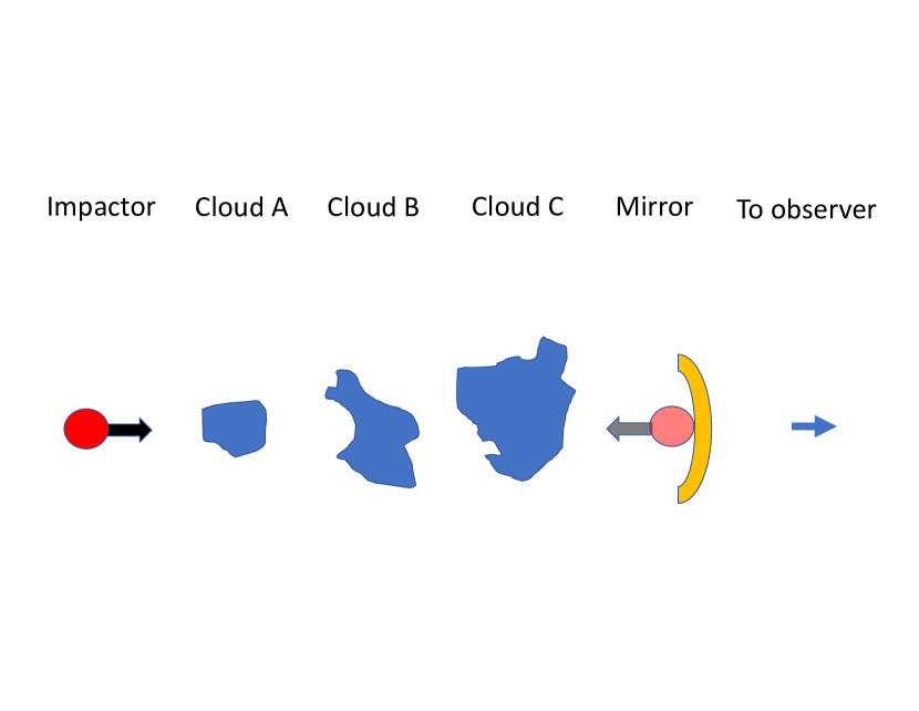
Figure 23: A model of temporally-reversed pulse structure. An impactor (red circle) produces variable radiation as it travels through clouds (blue), and has its motion physically reversed by a mirror (yellow), so that it travels through the same material in reverse order (pink circle).

Note that this model produces the proper temporal signature if one impactor travels through multiple clouds, but not if multiple impactors (1 and 2) travel through these same clouds and are reflected to travel back through the clouds in reverse order. This scenario produces events in a non-reversible chronological order (A1 A2 B1 B2 C1 C2 C1 C2 B1 B2 A1 A2) rather than in the reverse chronological order (A1 A2 B1 B2 C1 C2 C2 C1 B2 B1 A2 A1) and is thus not viable. A non-reversible chronological order is obtained for any number of impactors greater than one.

The mechanism for reversing the impactor motion is unknown, but might be due to a soliton reflecting off of a region characterized by higher opacity (e.g., Singh & Malik (2006)) or to charged particles reflecting off a region associated with a high magnetic field density, such as a magnetic mirror or magnetic bottle (e.g., Barkov et al. (2018)).

Our kinematic model can be related to the standard GRB model if we assume that the mirror results from increased density (e.g., Levinson & Begelman (2013)) and/or tightly-wound magnetic fields in the head of a GRB jet (e.g., Lynden-Bell (1996)), and that the clouds are density or magnetic structures formed within the jet. These clouds would move toward the head of the jet as the jet head plows into an external medium (e.g., Hardee et al. (1998); Hardee (2000); Agudo et al. (2001); Kato et al. (2004); Porth (2013); Martí (2015); Martí et al. (2016)). The impactor could be a superluminal event generated by the central engine.

Interactions between the impactor and the clouds cannot be seen in emitting regions that move away from the observer, due to relativistic motion. However, all forward and reverse interactions can be observed if the emitting regions (clouds and mirror) are moving towards the observer. Thus, the impactor could change its direction of motion in the mirror’s reference frame while still be moving towards the observer. Clouds catching up with the impactor would cause another round of radiation to be emitted. The temporal compression of the residuals on the pulse rise would indicate relativistic blueshifted motion toward the observer prior to reflection while the stretching observed during the pulse decay would indicate less-pronounced blueshifted motion toward the observer following reflection.

A gradient of cloud structure, density, and/or magnetic field close to the mirror might also explain increased residual amplitudes close to the time of reflection. Increased interactions should lead to increased residual amplitudes.

In a GRB with multiple pulses, this kinematic model requires either that two or more impactors strike a single mirror at different times, or that a single impactor somehow interacts with two or more mirrors as it moves through the jet. The single mirror/multiple impactor hypothesis can be explained in hypernova models of long GRBs, where multiple impactors might be emitted during the stellar collapse process (e.g., MacFadyen & Woosley (1999)), or in the cannonball GRB model (e.g., (Dar, 2006)), but it is not consistent with merging neutron star models of short GRBs, where repeated explosions from the central engine seem less likely. The single impactor/multiple mirror hypothesis seems unlikely in both long and short GRB scenarios, as the number of pulses is limited by the presence of a mirror that completely reflects ejecta. This model only works if multiple mirrors exist within the jet and if these mirrors are accessible to the impactor. We do not know how this situation might arise; perhaps isolated bubbles within the jet exist as a result of magnetic reconnection (Kato et al., 2004), and perhaps part of the impactor is somehow transmitted forward through each mirror in addition to the reflected part.

6.1.2 Model 2: Unaltered Motion of Impactor

A physical mirror is not required to explain the stretched and time-reversible pulse residuals. A more direct explanation is that a simple impactor moves constantly in one direction (presumably toward the observer) rather than one undergoing reflection and changing its direction of motion. In this case, interactions between the impactor and the clouds might produce the observed light curve structures if the clouds have some sort of radial bilateral symmetry (e.g., if they are distributed with cylindrical or spherical symmetry along the particle path). The increased residual amplitudes near the time of reflection might indicate an increased density or cloud size toward the center of the cloud distribution. This model, like the previous one, thus presupposes that structure exists within the jet. The model is shown in Figure 24.

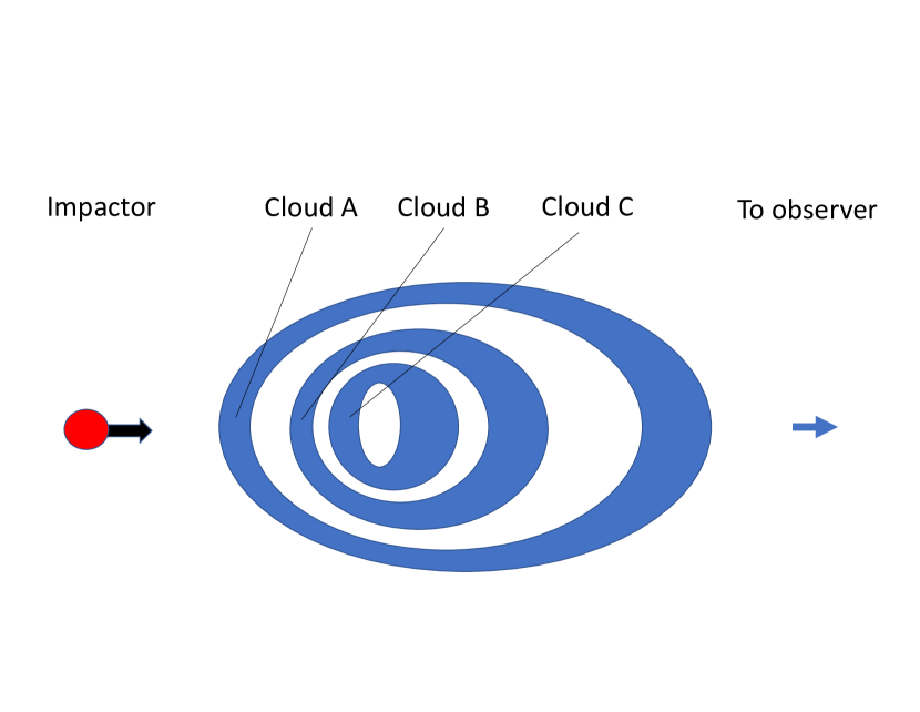
Figure 24: A model of temporally-reversed pulse structure. An impactor (red) produces variable radiation as it travels through axisymmetric, stretched clouds (blue).

Non-uniform flow is expected in an expanding jet due to instabilities in the accretion disk as well as to dynamics of the spout through which the jet flows (MacFadyen & Woosley, 1999). These instabilities likely depend on the angular momentum of the star, the accretion disk characteristics, the stellar mass, and the magnetic field. Variability in jet outflow can be caused both by instabilities at the central engine and those generated as the material passes through the star (Morsony et al., 2010).

Without knowing the form of GRB jet structure, it is not obvious why this proposed structure might cause the residual emission to stretch following the time of reflection (which corresponds to the center of the radial cloud distribution). It is possible that the motion of the impactor might compress the structure as it moves through it. However, any corresponding deceleration of the impactor should be gradual rather than abrupt as observed.

Note that again two or more impactors cannot produce the residuals seen in a single pulse, because the order of events is then irreversible. Suppose that interactions between the first impactor and symmetrically-distributed clouds A and B produce emission A1 and B1, respectively, and that interactions between the second impactor (moving closely behind the first) and the clouds similarly produce emission A2 and B2. The order of the episodes will not reverse once the impactors pass the center of the cloud distribution, and is thus not viable. In other words, the order of emission will be A1 A2 B1 B2 B1 B2 A1 A2 or something equally irreversible depending on the difference in time when each impactor interacts with the clouds.

Multi-pulsed bursts can be explained if each impactor produces its own pulse. In other words, two or more separate impactors can pass through the same set of clouds and produce different pulse/residual properties if the time between impactor arrivals at the cloud distribution is much longer than the time it takes the impactor to travel from cloud to cloud. Similarly, the reversible emission can be produced in separate pulses if one impactor passes through two isolated cloud distributions that are located long distances from one another.

6.1.3 Model 3: Bilaterally-Symmetric-Shaped Impactor

It is possible that the bilaterally-symmetric physical structure belongs to the impactor rather than to the clouds. In order to produce the time-reversed structure this model requires the interaction to take place within a single cloud, rather than with a distribution of clouds. The impactor could be a clump of material containing a bilaterally-symmetric density distribution, a bilaterally-symmetric distribution of streaming clumps of material, or a stream of bilaterally-symmetric distributed solitons. The mechanism that produces this impactor structure could again relate to instabilities in the accretion disk and/or in the jet spout (MacFadyen & Woosley, 1999).

The impactor distribution might also be produced magnetically through the linkage of a series of magnetic bottles or sheets in a process tied to jet collimation. Symmetry in the physical structure of an impactor might have to be matched by a uniformity of structure in the impacted material in order to produce the time-reversible pulse structure. Stretching of the wave would almost require an asymmetric impactor structure, with clumps being compressed on the leading side of the moving impactor and stretched on the trailing side (perhaps indicating compression of the impactor’s magnetic field in the direction of motion). This model is demonstrated in Figure 25.

This model provides a simple explanation for the observation of multiple GRB pulses. Either multiple impactors are ejected from the central engine (which is still a potential problem for merging neutron stars and short GRBs) or one impactor produces multiple pulses as it travels through multiple clouds.

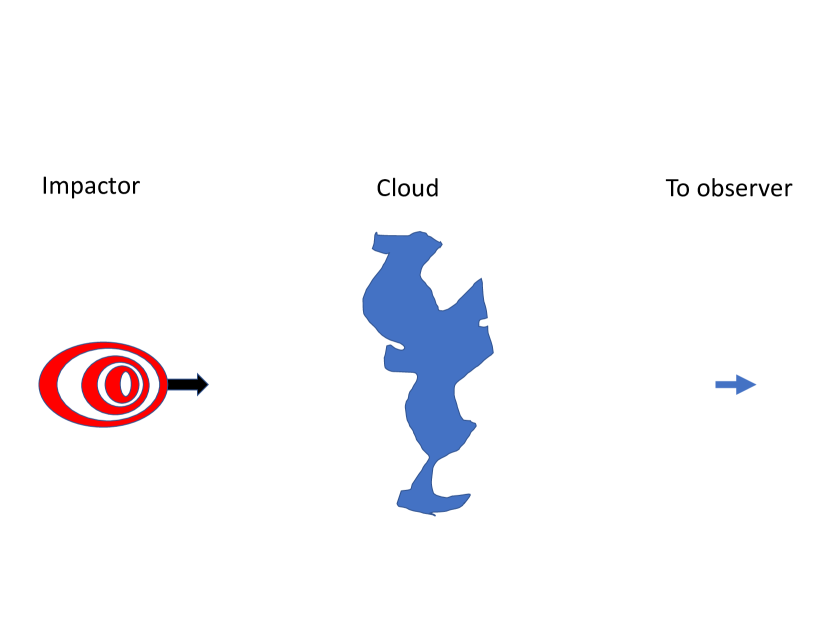
Figure 25: A model of temporally-reversed pulse structure. A bilaterally-symmetric impactor (red) produces variable radiation as it travels through a cloud (blue).

Kinematic models 2 and 3 are similar to one another, differing primarily in whether the physical structure responsible for producing the time-reversible and stretched residuals is found in the lower-velocity material (Model 2) or the higher-velocity material (Model 3). This is a minor difference from our perspective, since we do not presently know the origins of either the clouds or the impactor.

6.1.4 Model 4: Wavelike Instabilities Caused by Impactor

A time-reversible wave-like residual structure might also be produced from oscillations created when an impactor passes through a cloud medium. If the characteristics of the medium are spherically or cylindrically symmetric (for example, if the cloud density decreases towards the edges), so that they appear to be bilaterally symmetric to the observer, then the characteristics of the oscillations (e.g., frequency, amplitude) could change as the impactor passes through the cloud. Stretching of the residual wave might be caused by a factor such as a change in the cloud’s density gradient. Note that this model, like the previous two, preferentially favors interactions of a single impactor with one or more clouds. This appears to be a constraint imposed by the time-reversed residual structure. We do not know how these waves could be formed.

6.1.5 Other Models

Other astrophysical models seem improbable given the data. For example, variable high-energy lightcurves are often associated with flaring, orbital motion (e.g. compact binary stars), or rotation (e.g. pulsars). The wavelike residual structures do not seem to represent any sort of periodic motion (especially since the periods of the wavelike residual structures decrease before the time of reflection then increase after it). Nor do the patterned temporal sequences found in the residuals seem indicative of any sort of flaring process that would not involve orbital motion or rotation.

6.2 Comments on Radiation Mechanisms: Are the Residuals “Waves” or “Sub-Pulses?”

The residuals produced by subtracting the monotonic pulse model from the observed light curve produce a wavelike function that exceeds the monotonic light curve half the time and is less than it otherwise. If we want to model this behavior using standard radiation mechanisms, then half the time this behavior must represent emission in excess of the monotonic pulse whereas otherwise it must represent some process that also removes photons from the line-of-sight (e.g., absorption, scattering, polarization).

It is simpler to imagine a GRB physical process that only produces photons than one that rapidly and systematically alternates between producing photons and removing them from the line-of-sight. Our Occam’s Razor assumption that GRB emission should be explained by the fewest number of pulses led to the characterization of “pulses” as monotonic components overlaid by structure, which we found to be time-reversed and stretched. However, applying Occam’s Razor instead to GRB radiation mechanisms would suggest that “pulses” should be explained by emission processes alone rather than by emission processes combined with absorption, scattering, and/or polarization; this assumption requires each pulse to be composed of many smaller sub-pulses in order to account for the large and rapid intensity variations found in GRB emission episodes while always representing positive flux. Using this hypothesis that GRB light curves are formed only from monotonic sub-pulses might not allow us to find the time-reversed and stretched light curve structures. Is there some way to determine whether time-reversed and stretched residuals are an inherent characteristic of GRB pulse light curves or whether they are simply artifacts of assumptions and therefore of the fitting process?

In order to answer this question, we need to revert to simple monotonic pulse models rather than a “structured” pulse model. The literature is full of monotonic pulse models, each designed only to emit photons. In addition to the Norris et al. (2005) model used in this study, these models have taken many functional forms, including pulses with power law rises and decays (e.g. Norris et al. (1996); Lee et al. (2000a, b)), power-law rises and exponential decays (e.g., Jia & Qin (2005)), Gaussian rises and exponential decays (e.g., Stern & Svensson (1996)), Gaussian rises and decays (Bhat et al., 2012), and more complex rise and decay functions (e.g., Kocevski et al. (2003)). Each of these models by definition treats any structure that cannot be due to noise as a separate pulse. As indicated in Section 3, we have previously applied this approach ourselves, and have found that making this assumption forces each GRB in our sample to be composed of dozens of individual sub-pulses.

One of our sampled GRBs exhibits a light curve that is nearly time-reversible without any pulse-fitting or stretching. The decay portion of BATSE 249’s light curve (right panel of Figure 3) contains a time-reversed memory of events that happened during the rise portion of the light curve (we previously described this as being like a series of cutout paper dolls). This reversibility is present regardless of whether the emission episode is composed of a single structured pulse or many monotonic sub-pulses. However, the features responsible for making the time-reversibility recognizable are themselves structured because a strict monotonic interpretation would require almost every recognizable feature to be subdivided into multiple sub-pulses. The recognizable structures are not perfect mirrored images of one another, but they are more recognizable as reversible structures than they would be as sub-pulses, as a structure on the pulse rise will likely be deconstructed into a different number of sub-pulses than the corresponding structure on the pulse decay, due to the slightly different amplitudes and shapes of these non-identical features. Since time-reversibility is present in 249 regardless of whether or not the rise and decay portions contain equal numbers of matching sub-pulses, we conclude that the assumption of monotonicity is not required for time-reversibility to be present.

Time-reversibility is not as obvious in the light curves of the other five sample GRBs as it is in 249. It would be somewhat visible in 143p2 if the pulse’s rise was stretched to have a similar duration as the decay. In other words, asymmetry plays a role in disguising 143p2’s time-reversibility, and stretching the rise side by a fixed amount aligns rise side features with corresponding decay side features. However, even after stretching the rise side, some pulses do not exhibit temporal symmetry and require the time of reflection to be moved away from the pulse peak. These pulses also need to have flux subtrracted from the continuum underneath them until they match. A combination of stretching, flux-subtraction, and temporally offsetting removed flux from the center of the temporally-matched features seems generally sufficient to identify time-reversed structures. It is interesting to note that the amount of flux that should be removed corresponds to the flux found in a monotonic pulse, that the asymmetry of this pulse corresponds to the amount of stretching needed in the residuals, and that the alignment of the mirrored residuals is close to the peak of the fitted pulse.

We made a choice to fit emission episodes using a single monotonic pulse model based on an Occam’s Razor argument. Our choice was not based on the expectation that the residuals would produce a time-reversed and stretched structure. The time-reversed residuals belong to the structured component of the emission episode rather than to the monotonic component; it is almost impossible that we could have fine-tuned any monotonic function to produce these residuals if they had not already been present.

Perhaps these features represent some combination of structured sub-pulses rather than a wave (this model splits the difference between simple monotonic and structured monotonic pulse models). Demonstrating that structured sub-pulses somehow combine to form a time-reversible pulse still requires some pulse continuum to be excluded and removed. Going through the same sort of detailed flux balancing and removal process described above for simple monotonic pulses might make it possible for us to recover a time-reversible pulse composed of many structured monotonic sub-pulses, but the process would be complex, burst-dependent, and would involve carefully balancing all the sub-pulse properties as they are being extracted. The current process is much simpler. Occam’s Razor states that we should accept our original simple assumption of one pulse per emission episode, rather than something more complicated. We thus believe that the time-reversed and stretched residual structure is not an artifact of the fitting procedure, and that the radiation mechanisms required to explain GRB pulse physics require some combination of emission, absorption, scattering, and/or polarization.

7 Conclusions

We have shown that instrumental characteristics are quite capable of smearing out inherent GRB pulse structure, and of reducing complex structures to both the triple-peaked pulse structure found at moderate $S/N$ and the simple monotonic pulse structure found at low $S/N$. It is possible that all GRB pulses have complex structures, but these structures can only be studied in GRB pulses observed at high $S/N$. Basic properties of the monotonic part of the pulse such as duration, asymmetry and lag can still be reliably extracted from faint pulses using the Norris et al. (2005) pulse model. These properties do not entirely or adequately characterize GRB pulses without the addition of the Hakkila & Preece (2014) residual model. However, as resilient to $S/N$ variations as these monotonic pulse measurements are, they do not entirely or adequately characterize GRB pulses, which can have faint emission extending from long before the monotonic portion of the pulse begins until long after it ends.

We have chosen to avoid the smearing of intrinsic pulse structural properties caused by instrumental noise by studying a sample of bright, complex BATSE GRBs. Despite their complexity, we find that these pulses share behaviors that can potentially be used to characterize all GRB pulses. The most surprising result is that the residual structure, defined as the non-monotonic pulse component, is characterized by complex yet time-reversible behavior. This behavior can encompass multiple structures, can span a time considerably longer than the duration of the monotonic component, and can have amplitudes similar to that of the monotonic component. Each pulse appears to have only one time-reversible residual structure, indicating that it may be a defining characteristic of a GRB pulse.

Pulses generally evolve in a hard-to-soft manner. However, they undergo spectral re-hardening at the times of each residual peak. Some pulses undergo an extended re-hardening that lasts through much of the monotonic component. In at least one case, we demonstrate how this re-hardening is responsible for the phenomenon of negative spectral lags, even though the pulse containing it evolves from hard to soft.

The predictable behaviors of structure in GRB pulses allow us to more clearly identify pulses in GRB light curves. As a result, we find that many GRBs likely contain only a few pulses, even if their structural appearance makes it seem otherwise. We suggest that caution must be applied when interpreting the number of pulses and the characteristics of these pulses as they are used in pulse population studies. For example, Ramirez-Ruiz & Fenimore (2000) have concluded that internal shocks rather than external shocks are responsible for GRB pulses based on the relatively constant pulse durations found in multi-pulsed GRBs. From our perspective, the Ramirez-Ruiz & Fenimore (2000) pulse sample is predominately composed of complex single- or double-pulsed GRBs, rather than multi-pulsed GRBs, invalidating the reasons for their conclusions. Short GRBs (Hakkila et al., 2018) have also been found to contain only small numbers of structured pulses, and many of these sub-structures contain temporal symmetries (u-shaped, twin-peaked, etc. - similar to what has been found here). The light curves of short GRBs and long GRBs seem to differ primarily by temporal scale and hardness, but are similar in many other ways.

The existence of time-reversed pulse structure leads us to believe that physical models of GRB pulses must contain strong physical symmetries and an interaction with a single impactor. We have explored a number of simple kinematic models, and find that either the distribution of impacted material in a GRB jet must be bilateral-symmetrically distributed and impacted by a single impactor, a physical phenomenon is responsible for reversing the course of a single impactor, or a single impactor creates emission in bilateral-symmetrically distributed material as it passes through it.

The literature contains many descriptions of how structure might form in GRB light curves. This is often described as “variability” (although this term convolves variability due to multiple pulses with variability due to structure). The models explain variability in prompt emission as being due to internal shocks (e.g., Paczynski & Xu (1994); Rees & Meszaros (1994); Kobayashi et al. (1997); Daigne & Mochkovitch (1998); Bošnjak et al. (2009)), relativistic turbulence (e.g., Kumar & Narayan (2009); Lazar et al. (2009); Narayan & Kumar (2009)), mini-jets (e.g., Lyutikov & Blandford (2003); Yamazaki et al. (2004); Zhang & Zhang (2014)), fluctuations in black-hole hyper-accretion disks (e.g., Lin et al. (2016)) or fluctuations in accretion disk magnetic fields (Lloyd-Ronning et al., 2016). None of these models predicts time-symmetric and stretched temporal structures, and few associate variability specifically with spectral re-hardening. Thus, the observations reported here provide new and potentially useful constraints on GRB central engines and jet structure.

Application of Occam’s Razor leads us to believe that the time-reversed and stretched residual structure is more appropriately described by a single monotonic pulse overlaid by a time-reversible and stretched residual wave structure than it is by a large number of appropriately-distributed monotonic sub-pulses. From this we conclude that the radiation mechanism responsible for producing GRB pulses is not solely due to emission, but is instead due to some combination of emission and photon removal along the line-of-sight.

Two of the six GRBs in our study exhibit multiple pulses. Some GRB pulses overlap temporally (see Figure 22); this implies either that distributions of impacted material can lie close together spatially or that multiple impactors can interact with a single distribution of material on timescales shorter than the interaction times.

The results derived here have been obtained from a small sample of bright GRB pulses. High $S/N$ and good time resolution seem to be necessary instrumental requirements for identifying and extracting time-reversible and stretched features. As many as 100 BATSE pulses with 64-ms resolution and having $S/N>25$ might be characterized by complex light curves potentially capable of exhibiting these features. We are currently working to increase the size of our sample by studying more bright BATSE bursts. GRBs observed by other experiments may also exhibit these features, although our potential success in observing them depends on their instrumental properties. For example, Fermi’s GBM has a smaller surface area than BATSE but has good $S/N$ and excellent time resolution. Swift’s BAT has a similar surface area to BATSE and excellent $S/N$, but operates in a noisier, lower-energy regime. We recognize that not all bright GRB pulses may exhibit these behaviors, and thus make no claims about how generic our results are. However, the consistency of our results suggests that we are one step closer to understanding the physics of cosmic gamma-ray bursts.

References

- Agudo et al. (2001) Agudo, I., Gómez, J.-L., Martí, J.-M., et al. 2001, ApJ, 549, L183
- Band (1997) Band, D. L. 1997, ApJ, 486, 928
- Barkov et al. (2018) Barkov, M. V., Lyutikov, M., Klingler, N., & Bordas, P. 2018, arXiv:1804.07341
- Beloborodov (2000) Beloborodov, A. M. 2000, ApJ, 539, L25
- Beloborodov (2010) Beloborodov, A. M. 2010, MNRAS, 407, 1033
- Beloborodov (2011) Beloborodov, A. M. 2011, ApJ, 737, 68
- Bhat et al. (1994) Bhat, P. N., Fishman, G. J., Meegan, C. A., et al. 1994, ApJ, 426, 604
- Bhat et al. (2012) Bhat, P. N., Briggs, M. S., Connaughton, V., et al. 2012, ApJ, 744, 141
- Bošnjak et al. (2009) Bošnjak, Ž., Daigne, F., & Dubus, G. 2009, A&A, 498, 677
- Burgess (2014) Burgess, J. M. 2014, MNRAS, 445, 2589
- Chakrabarti et al. (2018) Chakrabarti, A., Chaudhury, K., Sarkar, S. K., & Bhadra, A. 2018, Journal of High Energy Astrophysics, 18, 15
- Cheng et al. (1995) Cheng, L. X., Ma, Y. Q., Cheng, K. S., Lu, T., & Zhou, Y. Y. 1995, A&A, 300, 746
- Dai et al. (2017) Dai, Z., Daigne, F., & Mészáros, P. 2017, Space Sci. Rev., 212, 409
- Daigne & Mochkovitch (1998) Daigne, F., & Mochkovitch, R. 1998, MNRAS, 296, 275
- Dar (2006) Dar, A. 2006, Chinese Journal of Astronomy and Astrophysics Supplement, 6, 301
- Drenkhahn & Spruit (2002) Drenkhahn, G., & Spruit, H. C. 2002, A&A, 391, 1141
- Fenimore et al. (1996) Fenimore, E. E., Madras, C. D., & Nayakshin, S. 1996, ApJ, 473, 998
- Ford et al. (1995) Ford, L. A., et al. 1995, ApJ, 439, 307
- Giannios & Spruit (2005) Giannios, D., & Spruit, H. C. 2005, A&A, 430, 1
- Golenetskii et al. (1983) Golenetskii, S. V., Mazets, E. P., Aptekar, R. L., & Ilinskii, V. N. 1983, Nature, 306, 451
- Goodman (1986) Goodman, J. 1986, ApJ, 308, L47
- Hakkila et al. (2008) Hakkila, J., et al. 2008, ApJ, 677, L81
- Hakkila & Nemiroff (2009) Hakkila, J., & Nemiroff, R. J. 2009, ApJ, 705, 372
- Hakkila & Preece (2011) Hakkila, J., & Preece, R. D. 2011, ApJ, 740, 104
- Hakkila & Preece (2014) Hakkila, J., & Preece, R. D. 2014, ApJ, 783, 88
- Hakkila et al. (2015) Hakkila, J., Lien, A., Sakamoto, T., et al. 2015, ApJ, 815, 134
- Hakkila et al. (2018) Hakkila, J., Horváth, I., Hofesmann, E., & Lesage, S. 2018, ApJ, 855, 101
- Hardee et al. (1998) Hardee, P. E., Rosen, A., Hughes, P. A., & Duncan, G. C. 1998, ApJ, 500, 599
- Hardee (2000) Hardee, P. E. 2000, ApJ, 533, 176
- Horack (1991) Horack, J. M. 1991, Development of the Burst And Transient Source Experiment (BATSE)., by Horack, J. M.. National Aeronautics and Space Administration, Washington, DC (USA), Sep 1991, 324 p.,,
- Jia & Qin (2005) Jia, L.-W., & Qin, Y.-P. 2005, ApJ, 631, L25
- Kargatis et al. (1994) Kargatis, V. E., Liang, E. P., Hurley, K. C., et al. 1994, ApJ, 422, 260
- Kato et al. (2004) Kato, Y., Hayashi, M. R., & Matsumoto, R. 2004, ApJ, 600, 338
- Kumar & Narayan (2009) Kumar, P., & Narayan, R. 2009, MNRAS, 395, 472
- Lazar et al. (2009) Lazar, A., Nakar, E., & Piran, T. 2009, ApJ, 695, L10
- Kobayashi et al. (1997) Kobayashi, S., Piran, T., & Sari, R. 1997, ApJ, 490, 92
- Kocevski et al. (2003) Kocevski, D., Ryde, F., & Liang, E. 2003, ApJ, 596, 389
- Lee et al. (2000a) Lee, A., Bloom, E. D., & Petrosian, V. 2000, ApJS, 131, 1
- Lee et al. (2000b) Lee, A., Bloom, E. D., & Petrosian, V. 2000, ApJS, 131, 21
- Levinson & Begelman (2013) Levinson, A., & Begelman, M. C. 2013, ApJ, 764, 148
- Liebig et al. (2015) Liebig, C., D’Ago, G., Bozza, V., & Dominik, M. 2015, MNRAS, 450, 1565
- Lin et al. (2016) Lin, D.-B., Lu, Z.-J., Mu, H.-J., et al. 2016, MNRAS, 463, 245
- Lloyd-Ronning et al. (2016) Lloyd-Ronning, N. M., Dolence, J. C., & Fryer, C. L. 2016, MNRAS, 461, 1045
- Lynden-Bell (1996) Lynden-Bell, D. 1996, MNRAS, 279, 389
- Lyutikov & Blandford (2003) Lyutikov, M., & Blandford, R. 2003, arXiv:astro-ph/0312347
- MacFadyen & Woosley (1999) MacFadyen, A. I., & Woosley, S. E. 1999, ApJ, 524, 262
- Martí (2015) Martí, J.-M. 2015, MNRAS, 452, 3106
- Martí et al. (2016) Martí, J. M., Perucho, M., & Gómez, J. L. 2016, ApJ, 831, 163
- Morsony et al. (2010) Morsony, B. J., Lazzati, D., & Begelman, M. C. 2010, ApJ, 723, 267
- Meszaros et al. (1993) Meszaros, P., Laguna, P., & Rees, M. J. 1993, ApJ, 415, 181
- Narayan & Kumar (2009) Narayan, R., & Kumar, P. 2009, MNRAS, 394, L117
- Norris et al. (1986) Norris, J. P., Share, G. H., Messina, D. C., et al. 1986, ApJ, 301, 213
- Norris et al. (1996) Norris, J. P., Nemiroff, R. J., Bonnell, J. T., et al. 1996, ApJ, 459, 393
- Norris et al. (2000) Norris, J. P., Marani, G. F., & Bonnell, J. T. 2000, ApJ, 534, 248
- Norris et al. (2005) Norris, J. P., Bonnell, J. T., Kazanas, D., Scargle, J. D., Hakkila, J., & Giblin, T. W. 2005, ApJ, 627, 324
- Paciesas et al. (1992) Paciesas, W. S., Pendleton, G. N., Kouveliotou, C., et al. 1992, American Institute of Physics Conference Series, 265, 190
- Paciesas et al. (2000) Paciesas, W. S., Meegan, C. A., Pendleton, G. N., et al. 2000, VizieR Online Data Catalog, 9020,
- Paczynski (1986a) Paczynski, B. 1986, ApJ, 304, 1
- Paczynski (1986b) Paczynski, B. 1986, ApJ, 308, L43
- Panaitescu et al. (1999) Panaitescu, A., Spada, M., & Mészáros, P. 1999, ApJ, 522, L105
- Pe’er et al. (2006) Pe’er, A., Mészáros, P., & Rees, M. J. 2006, ApJ, 642, 995
- Pe’er (2008) Pe’er, A. 2008, ApJ, 682, 463
- Pendleton et al. (1996) Pendleton, G. N., Mallozzi, R. S., Paciesas, W. S., et al. 1996, ApJ, 464, 606
- Peng et al. (2007) Peng, Z.-Y., Lu, R.-J., Qin, Y.-P., & Zhang, B.-B. 2007, Chinese J. Astron. Astrophys., 7, 428
- Porth (2013) Porth, O. 2013, MNRAS, 429, 2482
- Paczynski & Xu (1994) Paczynski, B., & Xu, G. 1994, ApJ, 427, 708
- Preece et al. (1998) Preece, R. D., Briggs, M. S., Mallozzi, R. S., et al. 1998, ApJ, 506, L23
- Ramirez-Ruiz & Fenimore (2000) Ramirez-Ruiz, E., & Fenimore, E. E. 2000, ApJ, 539, 712
- Rees & Meszaros (1994) Rees, M. J., & Meszaros, P. 1994, ApJ, 430, L93
- Rees & Mészáros (2005) Rees, M. J., & Mészáros, P. 2005, ApJ, 628, 847
- Richardson et al. (1996) Richardson, G., Koshut, T., Paciesas, W., & Kouveliotou, C. 1996, American Institute of Physics Conference Series, 384, 87
- Roychoudhury et al. (2014) Roychoudhury, A., Sarkar, S. K., & Bhadra, A. 2014, ApJ, 782, 105
- Ryde et al. (2011) Ryde, F., Pe’er, A., Nymark, T., et al. 2011, MNRAS, 415, 3693
- Ryde (2005) Ryde, F. 2005, A&A, 429, 869
- Sari & Piran (1997) Sari, R., & Piran, T. 1997, ApJ, 485, 270
- Schaefer (2004) Schaefer, B. E. 2004, ApJ, 602, 306
- Singh & Malik (2006) Singh, D. K., & Malik, H. K. 2006, Physics of Plasmas, 13, 082104
- Spruit et al. (2001) Spruit, H. C., Daigne, F., & Drenkhahn, G. 2001, A&A, 369, 694
- Stern & Svensson (1996) Stern, B. E., & Svensson, R. 1996, ApJ, 469, L109
- Tavani (1995) Tavani, M. 1995, Ap&SS, 231, 181
- Thompson (1994) Thompson, C. 1994, MNRAS, 270, 480
- Ukwatta et al. (2010) Ukwatta, T. N., Stamatikos, M., Dhuga, K. S., et al. 2010, ApJ, 711, 1073
- Wheaton et al. (1973) Wheaton, W. A., Ulmer, M. P., Baity, W. A., et al. 1973, ApJ, 185, L57
- Yamazaki et al. (2004) Yamazaki, R., Ioka, K., & Nakamura, T. 2004, ApJ, 607, L103
- Zhang et al. (2009) Zhang, B., Zhang, B.-B., Virgili, F. J., et al. 2009, ApJ, 703, 1696
- Zhang & Yan (2011) Zhang, B., & Yan, H. 2011, ApJ, 726, 90
- Zhang & Zhang (2014) Zhang, B., & Zhang, B. 2014, ApJ, 782, 92