Subvacuum effects on light propagation

Abstract

Subvacuum effects arise in quantum field theory when a classically positive quantity, such as the local energy density, acquires a negative renormalized expectation value. Here we investigate the case of states of the quantized electromagnetic field with negative mean-squared electric field, and their effects on the propagation of light pulses in a nonlinear dielectric material with a nonzero third-order susceptibility. We identify two distinct signatures of the subvacuum effect in this situation. The first is an increase in the speed of the pulse, which is analogous to the superluminal light propagation in gravity which can arise from negative energy density. This increase in speed leads to a phase shift which might be large enough to observe. The second effect is a change in the frequency and power spectra of the pulse. We identify a specific measure of the modified spectra which can signal the presence of a negative mean squared electric field. These ideas are implemented in the particular example of a wave guide filled with a nonlinear dielectric material.

I Introduction

A subvacuum effect in quantum field theory may be defined as a situation where a classically positive quantity, such as the energy density or the squared electric field, acquires a negative expectation value when the formally divergent part is subtracted. This can arise either in the presence of boundaries, such as the Casimir effect BM69 ; SF02 ; SF05 , or in a nonclassical quantum state, such as a squeezed vacuum state Caves . In flat spacetime, the relevant operator is taken to be normal-ordered, so its vacuum expectation value vanishes, and a locally negative expectation value represents a suppression of quantum fluctuations below the vacuum level, or a subvacuum effect. Negative energy density and its possible effects in gravity have been extensively studied in recent years. This includes proving various quantum inequality relations, which limit the magnitude and duration of subvacuum effects ford78 ; ford91 ; fr95 ; fr97 ; flanagan97 ; FE98 ; pfenning01 ; fh05 . One particularly striking effect of negative energy density is its ability to increase the speed of light compared to its speed in the vacuum PSW ; Olum ; VBL . This can be viewed as a “Shapiro time advance”, and is the converse of the effect of positive energy, which produces the Shapiro time delay Shapiro . Of course, the gravitational effects of negative energy density are normally very small, so there is interest in finding analog effects in nongravitational systems which might be easier to observe in the laboratory. Some proposals which have been made in the past include effects of vacuum fluctuation suppression on spin systems fgo92 or on the decay rate of atoms in excited states FR11 . Another possibility involves the propagation of light in nonlinear materials, where electric field fluctuations could lead to fluctuations in the speed of light FDMS13 ; BDFS15 ; BDFR16 , and a negative mean squared electric field could increase the average speed of light in a material BDF14 . Here we focus attention upon the latter effect in a material with a nonzero third-order susceptibility, and will discuss two phenomenological signatures of the subvacuum effect. We consider a probe wave packet propagating through a region with a negative mean-squared background electric field, and show that the subvacuum effect produces both a phase advance of the packet, and particular features in its frequency and power spectra.

The wave equation of a probe field prepared in a single mode coherent state propagating in a nonlinear optical material is obtained in the next section, under certain conditions. It is shown that an applied background electric field prepared in a squeezed vacuum state couples to the nonlinearities of the medium and affects the motion of the probe field. Particularly, a phase shift occurs whose magnitude may be large enough to be observable. Section III deals with the influence of the quantum fluctuations of the background field on the spectrum of a propagating probe wave packet. Possible observable signatures related to subvacuum effects are presented in this section. In Sec. IV we explore these ideas in a model with a rectangular wave guide filled with a nonlinear dielectric. The results of the paper are summarized and discussed in Sec. V. Unless otherwise noted, we work in Lorentz-Heaviside units with $\hbar=c=1$, so $\epsilon_{0}=1$.

II Phase shift

We start with the wave equation for an electric field in a nonlinear dielectric material FDMS13 ,

$$\biggl{(}\nabla^{2}-\frac{\partial^{2}}{\partial t^{2}}\biggr{)}E_{i}=\frac{\partial^{2}}{\partial t^{2}}P_{i}\,,$$ (1)

where we assume that $\nabla\cdot\mathbf{E}=0$, and $P_{i}$ represents the $i$-th component of the polarization vector, whose power series expansion in the electric field is given by (see, for example, Ref. boyd2008 )

$$P_{i}=\chi_{ij}^{(1)}E_{j}+\chi_{ijk}^{(2)}E_{j}E_{k}+\chi_{ijkl}^{(3)}E_{j}E_{k}E_{l}+\cdots\,.$$ (2)

Here summation on repeated indices is understood. The coefficients $\chi_{ij}^{(1)}$ are the components of the linear susceptibility tensor, while $\chi_{ijk}^{(2)}$ and $\chi_{ijkl}^{(3)}$ are the components of the second- and third-order nonlinear susceptibility tensors, respectively. We will be interested in centrosymmetric materials, for which the $\chi_{ijk}^{(2)}$ coefficients are identically zero. Additionally, if we specialize to the case where the electric field propagates in the $x$-direction and is linearly polarized in the $y$-direction, we obtain

$$\biggl{[}\frac{\partial^{2}}{\partial x^{2}}-\epsilon\,\frac{\partial^{2}}{\partial t^{2}}\biggr{]}E=\chi_{yyyy}^{(3)}\frac{\partial^{2}}{\partial t^{2}}E^{3},$$ (3)

where we define $\epsilon=1+\chi^{(1)}_{yy}$. In order to keep the notation simpler, in what follows we will suppress the indices of the susceptibility coefficients.

Suppose the electromagnetic field is prepared in a quantum state such that only two modes are excited, which will be called the probe (mode 1) and background (mode 2) fields. Let the probe field be a coherent state of amplitude $z$ described by the state vector $|z\rangle$, and the background field be a single-mode squeezed vacuum state defined by $|\zeta\rangle$. In general, $z$ and $\zeta$ are complex parameters, but we take them to be positive real numbers for simplicity, and set $\zeta=r$. Let us denote the state of the electromagnetic field as $|\psi\rangle=|z\rangle|\zeta\rangle$. Ignoring all other modes, the electric field operator can be expanded as $\hat{E}={\cal E}_{1}\hat{a}_{1}+{\cal E}^{*}_{1}\hat{a}^{\dagger}_{1}+{\cal E}_{2}\hat{a}_{2}+{\cal E}^{*}_{2}\hat{a}^{\dagger}_{2},$ where ${\cal E}_{i}$ is the mode function for mode $i$, and $\hat{a}_{i}$ and $\hat{a}_{i}^{\dagger}$ are the corresponding annihilation and creation operators, respectively. As $\langle\psi|\hat{a}_{2}|\psi\rangle=\langle\zeta|\hat{a}_{2}|\zeta\rangle=0$, the expectation value of the electric field operator when the system is prepared in the state $|\psi\rangle$ is

$${\cal E}_{c}=\langle\psi|\hat{E}|\psi\rangle=z\,({\cal E}_{1}+{\cal E}^{*}_{1})$$ (4)

where ${\cal E}_{c}$ can be viewed as the classical probe field. Similarly, the expectation value of normal-ordered $\hat{E}^{3}$ is given by

$$\langle\psi|:\hat{E}^{3}:|\psi\rangle={{\cal E}_{c}}^{3}+3{\cal E}_{c}\langle{E_{q}}^{2}\rangle\,,$$ (5)

where

$$\langle{E_{q}}^{2}\rangle=\langle\zeta|:({\cal E}_{2}\hat{a}_{2}+{\cal E}^{*}_{2}\hat{a}^{\dagger}_{2})^{2}:|\zeta\rangle=2\sinh r\left[|{\cal E}_{2}|^{2}\sinh r-{\rm Re}\left({{\cal E}_{2}}^{2}\right)\cosh r\right]$$ (6)

is the mean value of the normal-ordered squared background electric field operator. The subvacuum effect arises when $\langle{E_{q}}^{2}\rangle<0$. Let the mode function for the background field be a plane wave of the form ${\cal E}_{2}(x,t)=E_{0}\,{\rm e}^{i(k_{b}x-\Omega t)}$, so it is propagating in the $+x$-direction with angular frequency $\Omega$. Then we have

$$\langle{E_{q}}^{2}\rangle=2E_{0}^{2}\,\sinh^{2}r\{1-\coth r\,\cos[2(k_{b}x-\Omega t)]\}\,.$$ (7)

Because $\coth r>1$, we will have regions where $\langle{E_{q}}^{2}\rangle<0$ which travel at speed $\Omega/k_{b}$ in the $+x$-direction. The magnitude and duration of the $\langle{E_{q}}^{2}\rangle<0$ regions are constrained by quantum inequalities fr97 ; FE98 of the form $\langle{E_{q}}^{2}\rangle>-C/\tau^{4}$, where $\tau$ is the temporal duration of the negative expectation value at one spatial point, and $C$ is a positive constant smaller than one. The essential physical content of these inequalities is that there is an inverse relation between how negative $\langle{E_{q}}^{2}\rangle$ is, and how long the negative region can persist. In the case of Eq. (7), $\tau\lesssim 1/\Omega$ and states with $r\approx O(1)$ come closest to saturating the quantum inequality bounds KF18 . A generalization of Eq. (7) to a multimode example is given in Sec. IV. In the Appendix, it is shown that this example satisfies a quantum inequality.

The wave equation for the classical field ${\cal E}_{c}$ is obtained after using the above results in the quantum expectation value of Eq. (3), and becomes

$$\left[\frac{\partial^{2}}{\partial x^{2}}-\left(\epsilon+3\chi^{(3)}\langle{E_{q}}^{2}\rangle\right)\frac{\partial^{2}}{\partial t^{2}}\right]{\cal E}_{c}=\chi^{(3)}\frac{\partial^{2}}{\partial t^{2}}{{\cal E}_{c}}^{3}\,,$$ (8)

where we have assumed that the classical probe field varies rapidly compared to the background field. Let us consider the case where the cubic term on the right hand side of this equation may be neglected, so ${\cal E}_{c}$ approximately satisfies the linear equation

$$\left[\frac{\partial^{2}}{\partial x^{2}}-\left(\epsilon+3\chi^{(3)}\langle{E_{q}}^{2}\rangle\right)\frac{\partial^{2}}{\partial t^{2}}\right]{\cal E}_{c}\approx 0\,.$$ (9)

Then over a region small compared to the wavelength of the background field, so $\langle{E_{q}}^{2}\rangle$ is approximately constant, this equation describes waves with a phase velocity of $v_{\rm eff}$, where

$$v_{\rm eff}=\frac{1}{\sqrt{\epsilon+3\chi^{(3)}\langle{E_{q}}^{2}\rangle}}\approx v_{0}\left(1-\frac{3\chi^{(3)}}{2\epsilon}\langle{E_{q}}^{2}\rangle\right)\,.$$ (10)

Here $v_{0}=1/\sqrt{\epsilon}$ is the phase velocity in the absence of the background field, and we have assumed $\chi^{(3)}|\langle{E_{q}}^{2}\rangle|\ll 1$. In regions where $\langle{E_{q}}^{2}\rangle<0$, we have that the speed of the probe field is increased, $v_{\rm eff}>v_{0}$, although $v_{\rm eff}$ is still less than the speed of light in vacuum. This is the analog of the superluminal propagation of light in the presence of negative energy density in general relativity.

Consider a wave packet solution of the linearized equation for ${\cal E}_{c}$ of the form

$${\cal E}_{c}(x,t)=F(kx-\omega_{0}t)\,{\rm e}^{i(kx-\omega_{0}t)}\,,$$ (11)

where $F$ is an envelope function which varies more slowly than the exponential factor. In writing this form, we have assumed that dispersion can be ignored over the bandwidth of the wave packet, so that both the phase and group velocities are approximately $v_{\rm eff}=\omega_{0}/k$. If $\omega_{0}\gg\Omega$, we can select the envelope function so that the entire packet lies in a region where $\langle{E_{q}}^{2}\rangle$ is both negative and approximately constant, as illustrated in Fig. 1.

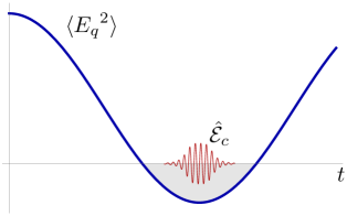
Figure 1: Illustration of the probe wave packet in a region where $\langle{E_{q}}^{2}\rangle$ is negative.

Further, let $\Omega/k_{b}\approx v_{0}$ so that this region moves at the same speed as does the wave packet. This is possible if $\epsilon(\Omega)\approx\epsilon(\omega_{0})$. Note that this does not require that $\epsilon(\omega)$ be constant over the entire interval from $\Omega$ to $\omega_{0}$. If these conditions are satisfied, then the probe packet moves together with the region where $\langle{E_{q}}^{2}\rangle<0$. This will allow the phase shift effect of the background field on the wave packet to accumulate.

The effect with which we are dealing is quite different from the apparent superluminal propagation which can arise in a region of anomalous dispersion, as can occur in atomic vapors Akulshin . The latter effect occurs when the index of refraction is changing rapidly as a function of frequency and where the group and phase velocities can be very different from one another and from the signal velocity. This is also a frequency region where absorption is large, and pulse shapes can change rapidly. None of these features apply in the effect we are describing.

Note that as the wave packet enters a region where $\langle{E_{q}}^{2}\rangle\not=0$, the peak frequency $\omega_{0}$ is unchanged, but the wavenumber changes from $k=k_{0}=\omega_{0}/v_{0}$ to

$$k=\frac{\omega_{0}}{v_{\rm eff}}\approx k_{0}\left(1+\frac{3\chi^{(3)}}{2\epsilon}\langle{E_{q}}^{2}\rangle\right)\,.$$ (12)

After a travel distance of $\Delta x=d$, this leads to a phase shift of the packet of

$$\Delta\varphi=(k-k_{0})\,d\approx 3\frac{\chi^{(3)}}{2\epsilon}\langle{E_{q}}^{2}\rangle\,k_{0}\,d=3\pi\frac{\chi^{(3)}}{\sqrt{\epsilon}}\langle{E_{q}}^{2}\rangle\left(\frac{d}{\lambda}\right)\,,$$ (13)

where $\lambda=2\pi\sqrt{\epsilon}/k_{0}$ is the wavelength of the probe field in the absence of the background field. To estimate the possible magnitude of this phase shift, we may use

$$\Delta\varphi\approx\frac{1}{\sqrt{\epsilon}}\left(\frac{\chi^{(3)}}{3\times 10^{-19}{\rm m^{2}V^{-2}}}\right)\left(\frac{\langle{E_{q}}^{2}\rangle}{1(\mu{\rm m})^{-4}}\right)\left(\frac{d}{10{\rm m}}\right)\left(\frac{0.1\mu{\rm m}}{\lambda}\right)\,.$$ (14)

The conversion to SI units is aided by noting that in our units $\epsilon_{0}=1$, which implies that $1V\approx 1.67\times 10^{7}{\rm m}^{-1}$.

We can see from Eq. (14) that if a sufficiently large travel distance $d$ can be arranged, then a potentially observable phase shift could result. Recall that this result was derived assuming that the nonlinear term in Eq. (8) can be neglected. This seems to require that ${{\cal E}_{c}}^{2}\ll|\langle{E_{q}}^{2}\rangle|$, and hence that $z\ll 1$. This in turn requires that the mean number of photons in the probe wave packet be small compared to one. Nonetheless, it may be possible to build up an interference pattern with an extremely low count rate, but a long integration time. Another possibility is that one might be able to take advantage of the dependence of the phase shift upon the background field even if the effect of the nonlinear term is not negligible.

III Effects on the spectrum of the probe wave packet.

III.1 Frequency spectrum of the probe field

Let

$$f(x,t)=\frac{3\chi^{(3)}}{2\epsilon}\,\langle{E_{q}}^{2}\rangle(x,t)\,,$$ (15)

so that Eq. (10) becomes $v_{\rm eff}\approx v_{0}\,[1-f(x,t)]$. We can write an approximate WKB solution of Eq. (9) as

$${\cal E}_{c}(x,t)={\cal E}_{0}{\rm e}^{ik_{0}\left[x-v_{0}\left(1-f\right)t\right]}\approx{\cal E}_{0}{\rm e}^{i\left(k_{0}x-\omega_{0}t\right)}\left(1+i\omega_{0}ft\right)\,,$$ (16)

where in the last step we assume $\left|f(x,t)\right|\omega_{0}t\ll 1$. When the background field is described by a single plane wave mode state, as in Eq. (7), $f(x,t)$ has the form

$$f(x,t)=\alpha+\beta\cos\left[2\left(k_{b}x-\Omega t\right)\right]\,,$$ (17)

where $\alpha>0$ and $\beta$ are constants. In the case of a squeezed vacuum state, as in Eq. (7), we have $|\beta|>\alpha$ and regions where $\langle{E_{q}}^{2}\rangle<0$. However, the form of Eq. (17) could hold for a broader range of states, including more classical states where $\alpha>|\beta|$ and $\langle{E_{q}}^{2}\rangle>0$ everywhere. Here we show that there are features in the frequency spectrum of the probe wave packet which can distinguish these two cases.

The frequency spectrum can be defined by a Fourier transform of the probe electric field at a fixed spatial location of the form

$$\hat{\cal E}_{c}(\omega)=\int_{-\infty}^{+\infty}{\rm e}^{i\omega t}{\cal E}_{c}(0,t)dt\,.$$ (18)

Use Eqs. (16) and (17) to find

$$\hat{\cal E}_{c}(\omega) = 2\pi{\cal E}_{0}\biggl{\{}\delta(\omega-\omega_{0})+\omega_{0}\alpha\delta^{\prime}(\omega-\omega_{0})$$ (19)

$$+\frac{1}{2}\omega_{0}\beta\bigl{[}\delta^{\prime}(\omega-\omega_{0}+2\Omega)+\delta^{\prime}(\omega-\omega_{0}-2\Omega)\bigr{]}\biggr{\}}\,,$$

where $\delta^{\prime}(\omega)=d\delta(\omega)/d\omega$ is the derivative of a $\delta$-function and $\omega_{0}=k_{0}v_{0}$. Equation (19) is the rather singular spectrum associated with the monochromatic solution, Eq. (16). A more realistic solution would be a wave packet with a finite bandwidth. The spectrum of such a solution can be obtained from Eq. (19) by replacing $\delta(\omega-\omega_{0})$ by $g(\omega-\omega_{0})$, a sharply peaked function with finite width and unit area, such as a Lorentzian function. The expected functional form of $g$ and its first derivative are plotted in Fig. 2.

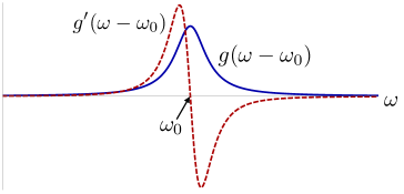
Figure 2: The shapes of the function $g(\omega-\omega_{0})$, described by a symmetric function centered at $\omega_{0}$, and its derivative, $g^{\prime}(\omega-\omega_{0})$, are illustrated.

In terms of the function $g$, the frequency spectrum for a wave packet becomes

$$\hat{\cal E}_{c}(\omega) = 2\pi{\cal E}_{0}\biggl{\{}g(\omega-\omega_{0})+\omega_{0}\alpha g^{\prime}(\omega-\omega_{0})$$ (20)

$$+\frac{1}{2}\omega_{0}\beta\bigl{[}g^{\prime}(\omega-\omega_{0}+2\Omega)+g^{\prime}(\omega-\omega_{0}-2\Omega)\bigr{]}\biggr{\}}\,.$$

Let us note some of the qualitative features of the spectrum in Eq. (20). When $\alpha=0$, there is a central peak at $\omega=\omega_{0}$. The term proportional to $g(\omega-\omega_{0})$ gives a symmetric contribution to this peak, but the term proportional to $\alpha$ produces a distortion which enhances the left ($\omega<\omega_{0}$) side and suppresses the right ($\omega>\omega_{0}$) side, if $\alpha>0$. To leading order, this is a shift of the peak to the left. Let $A_{L}$ and $A_{R}$ be the areas of the left and right sides, respectively, of $\omega=\omega_{0}$. The two terms in Eq. (20) proportional to $\beta$ produce side bands at $\omega=\omega_{0}\pm 2\Omega$. Each side band consists of a positive and a negative peak. Let $A_{S}$ be the area of one positive side band peak. All of these features are illustrated in Fig. 3.

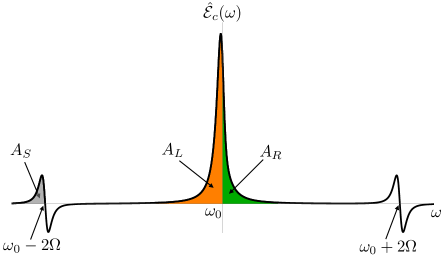
Figure 3: The frequency spectrum of a probe wave packet is illustrated. The effect of the background field is to produce a shift of the central peak, and two side bands at $\omega=\omega_{0}\pm 2\Omega$. The area of the central peak where $\omega<\omega_{0}$ is $A_{L}$ and that where $\omega>\omega_{0}$ is $A_{R}$. The area of one positive peak of a side band is $A_{S}$.

Note that $A_{S}$ may be written as

$$A_{S}=\left|\int_{-\infty}^{\omega_{0}-2\Omega}\hat{\cal E}_{c}(\omega)\,d\omega\right|=\pi\,{\cal E}_{0}\,\omega_{0}\,|\beta|\,g(0)\,$$ (21)

if ${\cal E}_{0}>0$. Similarly, the areas of the left and right sides of the central peak may be written as

$$A_{L}\approx\int_{\omega_{0}-n\Delta\omega_{p}}^{\omega_{0}}\hat{\cal E}_{c}(\omega)\,d\omega$$ (22)

and

$$A_{R}\approx\int_{\omega_{0}}^{\omega_{0}+n\Delta\omega_{p}}\hat{\cal E}_{c}(\omega)\,d\omega\,,$$ (23)

respectively. In the above integrals, $n$ is a number larger than one but $n\Delta\omega_{p}\ll 2\Omega$, where $\Delta\omega_{p}$ denotes the characteristic width of the function $g(\omega)$, i.e., the bandwidth of the probe field. Both $A_{L}$ and $A_{R}$ contain contributions from the symmetric $g(\omega-\omega_{0})$ term in Eq. (20). However, if we take the difference, $A_{L}-A_{R}$, these contributions cancel and only the contribution from the term proportional to $\alpha$ remains, leading to

$$A_{L}-A_{R}=4\pi{\cal E}_{0}\,\omega_{0}\,\alpha\,g(0)\,.$$ (24)

We may now use Eqs. (21) and (24) to write

$$\frac{|\beta|}{\alpha}=\frac{4A_{S}}{A_{L}-A_{R}}\,.$$ (25)

Recall that when $|\beta|>\alpha$, a subvacuum effect is present in that $\langle{E_{q}}^{2}\rangle<0$ somewhere, but when $|\beta|\leq\alpha$, the subvacuum effect is absent. Equation (25) shows how detailed features in the frequency spectrum of the probe wave packet can distinguish between these two situations. Specifically, if $4A_{S}>A_{L}-A_{R}$, then $\langle{E_{q}}^{2}\rangle<0$ somewhere.

If $g(\omega)$ has the form of a Lorentzian function,

$$g(\omega)=\frac{\Delta\omega_{p}}{\pi(\Delta\omega_{p}{}^{2}+\omega^{2})}\,,$$ (26)

it follows that $A_{L}-A_{R}=4{\cal E}_{0}\omega_{0}\alpha/\Delta\omega_{p}$. As the central peak is described by $2\pi{\cal E}_{0}g(\omega-\omega_{0})$, its area $A_{C}=A_{L}+A_{R}$ can be approximated by $A_{C}\approx 2\pi{\cal E}_{0}$. Hence,

$$\frac{A_{S}}{A_{C}}=\frac{1}{2\pi}\left(\frac{\omega_{0}}{\Delta\omega_{p}}\right)|\beta|,$$ (27)

and the asymmetry of the modified central peak can be described by means of

$$\frac{A_{L}-A_{R}}{A_{C}}=\frac{2}{\pi}\left(\frac{\omega_{0}}{\Delta\omega_{p}}\right)\alpha.$$ (28)

Here $\Delta\omega_{p}/\omega_{0}$ is the fractional line width of the probe field spectrum.

In the previous section, we described the probe pulse as a localized wavepacket which tracks the region of $\langle{E_{q}}^{2}\rangle<0$ in the background field, as illustrated in Fig. 1. Let $\tau_{b}=2\pi/\Omega$ denote the period of the background field and $\tau$ be the approximate temporal duration of the probe wavepacket, where $\tau<\tau_{b}$. This implies that the probe packet bandwidth, $\Delta\omega_{p}$, must to be larger than the background field angular frequency $\Omega$. Hence $(\Delta\omega_{p}/\omega_{0})>(\Omega/\omega_{0})$. However, the present discussion of the effects of the background field on the probe field spectrum does not require such an assumption. Here we may assume that the probe field is approximately monochromatic, and nonzero in both $\langle{E_{q}}^{2}\rangle<0$ and $\langle{E_{q}}^{2}\rangle>0$ regions, which allows $(\Delta\omega_{p}/\omega_{0})\ll 1$.

III.2 Power spectrum of the probe field

In this subsection, we turn our attention to features of the probe pulse power spectrum, which is likely to be easier to measure than is $\hat{\cal E}_{c}(\omega)$, the Fourier transform of the probe pulse electric field.

The energy per unit area per unit time carried by the probe pulse in vacuum is given by the Poynting vector $\vec{S}=\vec{\cal E}_{c}\times\vec{B}_{c}$. It follows that $|\vec{S}|=|\vec{\cal E}_{c}(x,t)|^{2}=|{\cal E}_{c}(x,t)|^{2}$. Setting $x=0$, the total energy per unit area in the probe pulse can be written as

$$u=\int_{-\infty}^{\infty}|{\cal E}_{c}(0,t)|^{2}dt=\frac{1}{2\pi}\int_{-\infty}^{\infty}|\hat{\cal E}_{c}(\omega)|^{2}d\omega=\int_{-\infty}^{\infty}P(\omega)d\omega,$$ (29)

where Parseval’s theorem was used in the second equality. In the above result we defined the power spectrum of the probe field as $P(\omega)=(1/2\pi)|\hat{\cal E}_{c}(\omega)|^{2}$. Using Eq. (20), we find

$$P(\omega) = 2\pi{\cal E}_{0}^{2}\biggl{\{}g(\omega-\omega_{0})^{2}+2\omega_{0}\alpha g(\omega-\omega_{0})g^{\prime}(\omega-\omega_{0})+\omega_{0}^{2}\alpha^{2}g^{\prime}(\omega-\omega_{0})^{2}$$ (30)

$$+\frac{1}{4}\omega_{0}^{2}\beta^{2}\bigl{[}g^{\prime}(\omega-\omega_{0}+2\Omega)^{2}+g^{\prime}(\omega-\omega_{0}-2\Omega)^{2}\bigr{]}\biggr{\}}\,,$$

where we assume that $2\Omega\gg\Delta\omega_{p}$, and thus cross terms involving $g^{\prime}(\omega-\omega_{0}\pm 2\Omega)$ can be neglected. Recall that $\Delta\omega_{p}$ is the approximate width of the central peak in Fig. 3, while $2\Omega$ is the separation of the sidebands from the central peak. The energy per unit area contained in the frequency interval $\omega_{1}\leq\omega\leq\omega_{2}$ becomes $\int_{\omega_{1}}^{\omega_{2}}P(\omega)d\omega$.

The power spectrum, $P(\omega)$, has several features which are similar to those of the frequency spectrum, which was illustrated in Fig. 3. Both spectra have the central peak displaced to the left of $\omega_{0}$, and sidebands at $\omega=\omega_{0}\pm 2\Omega$. The power spectrum is illustrated in Fig. 4 for the case that $g(\omega)$ is the Lorentzian function given in Eq. (26).

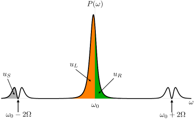
Figure 4: The power spectrum of the probe wave packet is here illustrated. The effect of the background field is to produce a shift of the central peak, and two double peaked side bands at $\omega=\omega_{0}\pm 2\Omega$. The area of the central peak where $\omega<\omega_{0}$ is $u_{L}$ and that where $\omega>\omega_{0}$ is $u_{R}$. The area of one positive peak of a side band is $u_{S}$.

The energy corresponding to the left and right sides of the central peak are given respectively by

$$u_{L}=\int_{\omega_{0}-n\Delta\omega_{p}}^{\omega_{0}}P(\omega)d\omega=\frac{{\cal E}_{0}^{2}}{2\Delta\omega_{p}}\left[1+\frac{4\omega_{0}\alpha}{\pi\Delta\omega_{p}}+\frac{\omega_{0}^{2}\alpha^{2}}{2\Delta\omega_{p}{}^{2}}\right],$$ (31)

$$u_{R}=\int_{\omega_{0}}^{\omega_{0}+n\Delta\omega_{p}}P(\omega)d\omega=\frac{{\cal E}_{0}^{2}}{2\Delta\omega_{p}}\left[1-\frac{4\omega_{0}\alpha}{\pi\Delta\omega_{p}}+\frac{\omega_{0}^{2}\alpha^{2}}{2\Delta\omega_{p}{}^{2}}\right].$$ (32)

Here we have used Eqs. (26) and (30). The asymmetry in the power spectrum about the central peak leads to the following fractional asymmetry in the energy distribution associated with the probe pulse,

$$\frac{u_{L}-u_{R}}{u_{C}}=\frac{4}{\pi}\left(\frac{\omega_{0}}{\Delta\omega_{p}}\right)\alpha$$ (33)

where $u_{C}\doteq{\cal E}_{0}^{2}/\Delta\omega_{p}$ is the energy in the central peak in the limit that $\alpha=0$. This expression is the analog of Eq. (28).

Finally, the area of a sideband depicted in Fig. 4. The energy carried by this part of the probe pulse is

$$u_{S}=\int_{-\infty}^{\omega_{0}-2\Omega}P(\omega)d\omega,$$ (34)

which leads to the fractional energy in the side band,

$$\frac{u_{S}}{u_{C}}=\frac{1}{16}\left(\frac{\omega_{0}}{\Delta\omega_{p}}\right)^{2}\beta^{2}.$$ (35)

In contrast to its analog for the frequency spectrum, Eq. (25), the above expression is quadratic both in ${\omega_{0}}/{\Delta\omega_{p}}$ and in $\beta$. Thus, if $(\omega_{0}/\Delta\omega_{p})|\beta|\ll 1$, measurement of $u_{S}/u_{0}$ could be difficult. In this case, the frequency spectrum might become a better probe of the presence of a subvacuum effect.

IV Mode functions in a rectangular wave guide

Let us now consider the specific case where an electromagnetic wave propagates in a rectangular wave guide whose cross section has dimensions $a$ and $b$, respectively. This example should provide a reasonable estimate of the magnitude of the effects expected in an optical fiber, but is easier to compute in detail. Suppose the boundaries are perfectly conducting and the inner region is filled with a dielectric material whose linear contribution to the electric permittivity is given by $\epsilon$. Solutions for the transverse electric (TE) modes propagating along the length of the wave guide can be expressed as Zangwill

$$B_{z} = B_{0}\,\cos\left(\frac{\pi mx}{a}\right)\,\cos\left(\frac{\pi ny}{b}\right)\,{\rm e}^{i\phi}\,,$$

$$B_{x} = \frac{ik}{\gamma^{2}}\;\frac{\partial B_{z}}{\partial x}\,,\qquad B_{y}=-\frac{ik}{\gamma^{2}}\;\frac{\partial B_{z}}{\partial y}\,,$$

$$E_{x} = \frac{\omega}{k}\,B_{y}\,,\qquad E_{y}=-\frac{\omega}{k}\,B_{x}\,,\qquad E_{z}=0\,.$$ (36)

In a change from the notation of previous sections, the wave is now propagating in the $+z$-direction. Here $\phi=kz-\omega t$, $k$ is the wavenumber, and $m$ and $n$ are positive integers,

$$\gamma=\sqrt{\left(\frac{\pi m}{a}\right)^{2}+\left(\frac{\pi n}{b}\right)^{2}}\,,$$ (37)

and

$$\omega=\frac{1}{\sqrt{\epsilon}}\,\sqrt{\gamma^{2}+k^{2}}$$ (38)

is the angular frequency of the mode.

These modes are normalized so that

$$\frac{1}{2}\int(\epsilon|{\bf E}|^{2}+|{\bf B}|^{2})d^{3}x=\frac{1}{2}\omega$$ (39)

is the zero point energy of a single mode. This determines the constant $B_{0}$ to be

$$B_{0}=\gamma\,\sqrt{\frac{2}{a\,b\,L\,\epsilon\,\omega}}\,,$$ (40)

where we impose periodic boundary conditions of length $L$ in the $z$-direction.

Now we generalize the treatment in Sec. II, and assume that the quantized electric field is prepared in a multimode squeezed vacuum state. We assume that the excited modes are associated with specific values of $m$ and of $n$, but a finite bandwidth of the wavenumber $k$. The mean-squared electric field is now given by

$$\langle{E_{q}}^{2}\rangle = \frac{4}{a\,b\,L\,\gamma^{2}}\,\left[\left(\frac{\pi m}{a}\right)^{2}\,\sin^{2}\left(\frac{\pi mx}{a}\right)\,\cos^{2}\left(\frac{\pi ny}{b}\right)+\left(\frac{\pi n}{b}\right)^{2}\,\cos^{2}\left(\frac{\pi mx}{a}\right)\,\sin^{2}\left(\frac{\pi ny}{b}\right)\,\right]$$ (41)

$$\times \sum_{k}\frac{\omega}{\epsilon}\sinh r_{k}\left[\sinh r_{k}-\cosh r_{k}\cos(kz-\omega t)\right],$$

where $r_{k}$ denotes the squeeze parameter corresponding to mode $k$. In the Appendix, we show that Eq. (41) satisfies a quantum inequality bound. Next we average $\langle{E_{q}}^{2}\rangle$ over the cross section of the wave guide, and let $\sum_{k}\rightarrow(L/2\pi)\int dk$, which leads to

$$\langle{E_{q}}^{2}\rangle=\frac{1}{2\pi\,a\,b}\,\int dk\,\frac{\omega}{\epsilon}\,\sinh r_{k}\left[\sinh r_{k}-\cosh r_{k}\cos(kz-\omega t)\right].$$ (42)

As before, this quantity will be negative when $\cos(kz-\omega t)\approx 1$. We assume that the squeeze parameter $r_{k}$ is different from zero only within a finite bandwidth $\Delta k$ about $k=\sqrt{\epsilon}\,\Omega$. Here the excited modes of the background field are in a finite angular frequency band peaked at $\omega=\Omega$. This leads to the value of $\langle{E_{q}}^{2}\rangle$ near its minimum of

$$\langle{E_{q}}^{2}\rangle_{\bf min}\approx-\frac{\Omega\,\Delta k}{2\pi\,a\,b\,\epsilon}\;\sinh r_{k}\left(\cosh r_{k}-\sinh r_{k}\right)\,.$$ (43)

Let us now examine the effects of the $\langle{E_{q}}^{2}\rangle<0$ regime on the probe pulse spectrum. The wave equation is the same as Eq. (9), but exchanging the variable $x$ by $z$. The WKB solution for ${\cal E}_{c}(z,t)$ is now given by Eq. (16) with

$$f(z,t)=-G\,\sinh r_{k}\left(\cosh r_{k}-\sinh r_{k}\right)\,,$$ (44)

where

$$G=\frac{3\chi^{(3)}\Omega\,\Delta k}{4\pi\,a\,b\,\epsilon^{2}}\,.$$ (45)

From Eq. (44), we identify the coefficients appearing in Eq. (17) to be $\alpha=G\sinh^{2}r_{k}$ and $|\beta|=G\sinh r_{k}\cosh r_{k}$. Note that both $\alpha$ and $|\beta|$ grow exponentially as $r_{k}$ increases, but their difference remains finite

$$|\beta|-\alpha=G\sinh r_{k}\left(\cosh r_{k}-\sinh r_{k}\right)=G(1-{\rm e}^{-2r_{k}})/2\approx\frac{1}{2}G\,\qquad r_{k}\gtrsim 1\,.$$ (46)

It is this difference which determines the magnitude of the subvacuum effect, which is our principal interest. Thus, we consider the case where $r_{k}$ is of order one in the region where it is nonzero. Then, in order of magnitude, we have

$$|\beta|\approx\alpha\approx|\beta|-\alpha\approx G\,.$$ (47)

The quantitiy $(\omega_{0}/\Delta\omega_{p})\,\alpha\approx(\omega_{0}/\Delta\omega_{p})\,|\beta|$, which appears in Eqs. (27), (28), (33), and (35) may be estimated from Eqs. (45) and (47) as

$$\left(\frac{\omega_{0}}{\Delta\omega_{p}}\right)\,|\beta|\approx\frac{1.0\times 10^{-8}}{\epsilon^{3}}\left(\frac{\chi^{(3)}}{3\times 10^{-19}{\rm m^{2}V^{-2}}}\right)\left(\frac{\Delta k}{\Omega}\right)\left(\frac{\omega_{0}}{\Delta\omega_{p}}\right)\ \left(\frac{1\mu{\rm m}}{\lambda_{b}}\right)^{2}\frac{(1\mu{\rm m})^{2}}{a\,b},$$ (48)

Recall that fractional asymmetry of both the frequency and power spectra, as well as the fractional area of the sidebands of the frequency spectra are all of the order of the quantity in Eq. (48), while the fractional area of the sidebands of the power spectrum is proportional to its square. Note that this quantity is proportional to the fractional bandwidth of the background field modes, ${\Delta k}/{\Omega}$, which need not be especially small, and inversely proportional to the fractional bandwidth of the probe field wavepacket, ${\Delta\omega_{p}}/{\omega_{0}}$, which can be very small. Hence, if we were to set $\omega_{0}/\Delta\omega_{p}\approx{\cal O}(10^{8})$, which is far from the narrowest possible line, we could have fractional results described by Eqs. (27) and (28) of order 1. However, the magnitude of $\omega_{0}/\Delta\omega_{p}$ is limited by the approximation used in the WKB solution given by Eq. (16), that requires $\omega_{0}ft<1$, and so $t<1/(\omega_{0}f)\approx 1/(\omega_{0}\alpha)\approx 1/(\omega_{0}|\beta|)$. Thus, the Taylor-expanded solution for ${\cal E}_{c}(x,t)$ is restricted to times obeying this condition, which puts a lower band on the bandwidth $\Delta\omega_{p}$ of $\Delta\omega_{p}\gtrsim 1/t>\omega_{0}\alpha$ (or $1/t>\omega_{0}|\beta|$). Hence, we need both $(\omega_{0}/\Delta\omega_{p})\alpha$ and $(\omega_{0}/\Delta\omega_{p})|\beta|$ to be smaller than unity. As a consequence, the various features of the frequency and power spectra, $A_{S}/A_{C}$, $(A_{L}-A_{R})/A_{C}$, $(u_{L}-u_{R})/u_{C}$, and $u_{S}/u_{C}$, given in Eqs. (27), (28), (33), and (35), respectively, all have to be small compared to one. However, if the spectra can be measured to sufficient accuracy, it may be possible to confirm the existence of the subvacuum effect.

V Summary and Discussion

In this paper, we have explored some consequences of a negative mean-squared electric field as an example of a subvacuum effect, one where quantum fluctuations are suppressed below the vacuum level. We consider the quantized electric field in a squeezed vacuum state, where $\langle{E_{q}}^{2}\rangle<0$ in some regions. This forms a background field which can increase the speed of propagation of a probe pulse in a nonlinear material with nonzero third-order susceptibility. This is an analog of the effect of negative energy density in general relativity, which can increase the effective speed of light.

Our primary concern is a search for systems where the increased light speed, or related effects, in a nonlinear dielectric might be observable. The fractional increase in light speed is typically both very small, perhaps of the order of $10^{-9}$, and transient. However, in Sec. II, we discussed the possibility that the probe pulse wavepacket can travel with the region of negative mean-squared electric field, and hence the phase shift from the speed increase might accumulate to a measurable magnitude. In Sec. III, we discussed the effects of a region where $\langle{E_{q}}^{2}\rangle<0$ on both the frequency spectrum and power spectrum of the probe pulse. We showed that the details of these spectra can carry information about whether the pulse has travelled through a region where $\langle{E_{q}}^{2}\rangle<0$. These ideas were developed further in Sec. IV in the context of pulses in a rectangular wave guide. This example allowed us to give some estimates of the magnitudes of the spectra features produced by a negative mean-squared electric field, which indicate that they might be observable.

Appendix A

In this appendix, we show that $\langle{E_{q}}^{2}\rangle$ in a rectangular wave guide satisfies the quantum inequality constraint derived in Refs. fr97 ; FE98 . This constraint is a lower bound of the form

$$\langle{E_{q}}^{2}\rangle\geq-\frac{C}{\tau^{4}}$$ (49)

where $0<C\lesssim 1$ and $\tau$ is the temporal duration of the negative mean squared electric field at a given point in space. The inequalities derived in Refs. fr97 ; FE98 generally require $\langle{E_{q}}^{2}\rangle$ to be averaged in time with a sampling function of characteristic width $\tau$. However, here we have a finite bandwidth of excited modes and can show that the results found in Sec. IV satisfy Eq. (49) without the need for time averaging.

We begin with Eq. (41), and note that $\langle{E_{q}}^{2}\rangle$ has its minimum value as a function of time when $\cos(kz-\omega t)=1$ and that the magnitudes of sine and cosine functions are bounded above by unity, so

$$\langle{E_{q}}^{2}\rangle\geq-\frac{1}{\pi\,a\,b}\,\int dk\;\frac{\omega}{\epsilon}\,.$$ (50)

Here we have used Eq. (37) and the fact [See Eq. (46).] that $\sinh r_{k}\left(\sinh r_{k}-\cosh r_{k}\right)\geq-\frac{1}{2}$. This bound is similar to the estimates given in Sec. IV , although here we do not assume a spatial average over the wave guide cross section. As before, we assume a bandwidth of excited modes in a wave number range $\Delta k$ peaked near $k=\bar{k}$, and hence in angular frequency near $\omega=\Omega=\sqrt{(\gamma^{2}+\bar{k}^{2})/\bar{\epsilon})}$, where $\bar{\epsilon}=\epsilon(\Omega)$. Because $\Delta k<\bar{k}<\Omega\sqrt{\bar{\epsilon}}$, we may write

$$\langle{E_{q}}^{2}\rangle\geq-\frac{\Omega^{2}}{\pi\,a\,b\,\sqrt{\bar{\epsilon}}}\,.$$ (51)

We have $\gamma\geq\pi m/a$ and $\gamma\geq\pi n/b$. Because both $m$ and $n$ are positive integers, we have

$$\frac{\Omega^{2}}{\pi\,a\,b\,\sqrt{\bar{\epsilon}}}\leq\frac{\gamma^{2}\,\Omega^{2}}{\pi^{3}\,m\,n\,\sqrt{\bar{\epsilon}}}\leq\frac{\gamma^{2}\,\Omega^{2}}{\pi^{3}\,\sqrt{\bar{\epsilon}}}<\frac{\sqrt{\bar{\epsilon}}\,\Omega^{4}}{\pi^{3}}\,.$$ (52)

Finally, because $\bar{\epsilon}$ is of order one, and $\tau$ is of order $1/\Omega$, we obtain the quantum inequality bound, Eq. (49).

References

- (1) L. S. Brown and G. J. Maclay, Vacuum stress between conducting plates: an image solution, Phys. Rev. 184, 1272 (1969).
- (2) V. Sopova and L. H. Ford, Energy density in the Casimir effect, Phys. Rev. D66, 045026 (2002); arXiv:quant-ph/0204125.
- (3) V. Sopova and L. H. Ford, Electromagnetic field stress tensor between dielectric half-spaces, Phys. Rev. D72, 033001 (2005); arXiv:quant-ph/0504143.
- (4) C. M. Caves, Quantum-mechanical noise in an interferometer, Phys. Rev. D 23, 1693 (1981).
- (5) L. H. Ford, Quantum coherence effects and the second law of thermodynamics, Proc. R. Soc. A364, 227 (1978).
- (6) L. H. Ford, Constraints on negative-energy fluxes, Phys. Rev. D43, 3972 (1991).
- (7) L. H. Ford and T. A. Roman, Averaged energy conditions and quantum inequalities, Phys. Rev. D51, 4277 (1995).
- (8) L. H. Ford and T. A. Roman, Restrictions on negative energy density in flat spacetime, Phys. Rev. D55, 2082 (1997).
- (9) E. E. Flanagan, Quantum inequalities in two-dimensional Minkowski spacetime, Phys. Rev. D56, 4922 (1997).
- (10) C. J. Fewster and S. P. Eveson, Bounds on negative energy densities in flat spacetime, Phys. Rev. D 58, 084010 (1998); arXiv:gr-qc/9805024.
- (11) M. J. Pfenning, Quantum inequalities for the electromagnetic field, Phys. Rev. D65, 024009 (2001).
- (12) C. J. Fewster and S. Hollands, Quantum energy inequalities in two-dimensional conformal field theory, Rev. Math. Phys. 17, 577 (2005).
- (13) R. Penrose, R. D. Sorkin and E. Woolgar, A positive mass theorem based on the focusing and retardation of null geodesics; arXiv:gr-qc/9301015.
- (14) K. D. Olum, Superluminal Travel Requires Negative Energies, Phys. Rev. Lett. 81, 3567 (1998); arXiv:gr-qc/9805003.
- (15) M. Visser, B. Bassett and S. Liberati, Perturbative superluminal censorship and the null energy condition, AIP Conf. Proc. 493, 301 (1999); arXiv:gr-qc/9908023.
- (16) I. I. Shapiro, Fourth test of general relativity, Phys. Rev. Lett. 13, 789 (1964).
- (17) L. H. Ford, P. G. Grove and A. C. Ottewill, Macroscopic detection of negative-energy fluxes, Phys. Rev. D46, 4566 (1992).
- (18) L. H. Ford and T. A. Roman, Effects of vacuum fluctuation suppression on atomic decay rates, Ann. Phys. 326 2294 (2011); arXiv:0907.1638.
- (19) L. H. Ford, V. A. De Lorenci, G. Menezes, and N. F. Svaiter, An analog model for quantum lightcone fluctuations in nonlinear optics, Ann. Phys. 329, 80 (2013); arXiv:1202.3099.
- (20) C. H. G. Bessa, V. A. De Lorenci, L. H. Ford and N. F. Svaiter, Vacuum lightcone fluctuations in a dielectric, Ann. Phys. 361, 293 (2015); arXiv:1408.6805.
- (21) C. H. G. Bessa, V. A. De Lorenci, L. H. Ford and C. C. H. Ribeiro, Model for lightcone fluctuations due to stress tensor fluctuations, Phys. Rev. D 93, 064067 (2016); arXiv:1602.03857.ean,
- (22) C. H. G. Bessa, V. A. De Lorenci, and L. H. Ford, Analog model for light propagation in semiclassical gravity, Phys. Rev. D 90, 024036 (2014); arXiv:1402.6285.
- (23) Robert W. Boyd, Nonlinear optics, 3rd ed. (Academic Press, New York, 2008).
- (24) A. Korolov and L. H. Ford, Maximal Subvacuum Effects: A Single Mode Example, Phys. Rev. D 98, 036020 (2018); arXiv:1805.07863.
- (25) For a recent review, see A. M. Akulshin and R. J. McLean, Fast light in atomic media, J. Opt. 12, 104001 (2010).
- (26) See, for example, A. Zangwill, Modern Electrodynamics, (Cambridge University Press, Cambridge, 2013) Sec. 19.4.