Volterra-Type Convolution of Classical Polynomials

Abstract.

We present a general framework for calculating the Volterra-type convolution of polynomials from an arbitrary polynomial sequence $\{P_{k}(x)\}_{k\geqslant 0}$ with $\deg P_{k}(x)=k$. Based on this framework, series representations for the convolutions of classical orthogonal polynomials, including Jacobi and Laguerre families, are derived, along with some relevant results pertaining to these new formulas.

1. Introduction

Convolution, as a fundamental operation, is commonly seen in many fields of sciences and engineering. Let $f:[a,b]\mapsto\mathbb{C}$ and $g:[c,d]\mapsto\mathbb{C}$ be two continuous integrable functions defined on intervals with a same length, that is $b-a=d-c$, where $a$ and $c$ are finite numbers while $b$ and $d$ can be finite or infinite. Their convolution $h(x)$ is a third function, given by

(1.1) $$h(x)=(f\ast g)(x)=\int_{c}^{x-a}f(x-t)g(t)\mathrm{d}t,~{}~{}~{}~{}~{}~{}~{}~{}~{}~{}~{}~{}x\in[a+c,a+d],$$

where the domain of $h(x)$, i.e. $[a+c,a+d]$, has the same length as those of $f(x)$ and $g(x)$. This operation is often denoted by an asterisk, as in (1.1).

When $b$ and $d$ are finite, $f(x)$ and $g(x)$ are compactly supported and can be mapped to the interval $[-1,1]$ via changes of variables and the convolution of the mapped versions of $f(x)$ and $g(x)$ differs from that of the original $f(x)$ and $g(x)$ by an affine transform only. Therefore, with slight abuse of our notation, we consider exclusively the convolution of two functions $f(x)$ and $g(x)$ that are defined on $[-1,1]$, that is,

(1.2) $$h(x)=(f\ast g)(x)=\int_{-1}^{x+1}f(x-t)g(t)\mathrm{d}t,~{}~{}~{}~{}~{}~{}~{}~{}~{}~{}~{}~{}x\in[-2,0],$$

where the convolution $h(x)$ is, in this case, a function on $[-2,0]$. Analogously, when $b$ and $d$ are infinities (1.1) becomes

(1.3) $$h(x)=(f\ast g)(x)=\int_{0}^{x}f(x-t)g(t)\mathrm{d}t,~{}~{}~{}~{}~{}~{}~{}~{}~{}~{}~{}~{}x\in[0,\infty],$$

up to a real Möbius transform. Note that the domains of the transformed $f(x)$, $g(x)$, and the convolution $h(x)$ all become $[0,\infty]$ in (1.3).

A powerful working paradigm that motivates this investigation and are commonly adopted in problems where functions considered are smooth is to replace $f(x)$ and $g(x)$ by their unique series representation in terms of classical orthogonal polynomials, e.g. Chebyshev or (weighted) Laguerre series for $f(x)$ and $g(x)$ in (1.2) and (1.3) respectively. In numerical computation, such series are usually truncated at certain degrees so that the finite series accurate to machine precision can serve as good approximants. In either case, the calculation of convolution integrals boils down to the convolution of polynomial series of finite or infinite degrees, or, further, to the convolution of classical orthogonal polynomials.

Suppose that $f_{M}(x)=\sum_{m=0}^{M}a_{m}P_{m}(x)$ and $g_{N}(x)=\sum_{n=0}^{N}b_{n}P_{n}(x)$ are two finite series of classical orthogonal polynomials. The convolution of $f_{M}(x)$ and $g_{N}(x)$ results in a degree $M+N+1$ polynomial $h_{M+N+1}(x)=\sum_{k=0}^{M+N+1}c_{k}P_{k}(x)$. In a recent work [12], it is shown that the convolution operator

$$V[f_{M}](g_{N})=h_{M+N+1}(x)=\int_{-1}^{x+1}f_{M}(x-t)g_{N}(t)\mathrm{d}t,~{}~{}~{}~{}~{}x\in[-2,0],$$

which is defined by $f_{M}(x)$ and applied to $g_{N}(x)$ can be represented as a $(M+N+2)\times(N+1)$ matrix $R$ so that the coefficients vector $\underline{c}=(c_{1},c_{2},\ldots,c_{M+N+1})^{T}$ equals the product of $R$ and the column vector $\underline{b}=(b_{1},b_{2},\ldots,b_{N})^{T}$. That is,

(1.4) $$\underline{c}=R\underline{b}.$$

In fact, this convolution matrix $R$ is constructed numerically using a four- or five-point recurrence relation satisfied by its entries. However, neither coefficients $\{c_{k}\}_{k=0}^{M+N+1}$ nor the entries of the convolution matrix $R$ are known explicitly.

In this paper, we derive explicit formulas for the convolution of two classical orthogonal polynomials of Jacobi or Laguerre families. The new results may hint us on the rich structure of convolution matrices $R$ and, in turn, shed light upon their fast construction as well as the design of fast algorithms for convolving polynomial series. On a different note, the results presented in this paper largely expand the collection of the existing convolution formulas comprised of those of Laguerre polynomials $L^{(0)}_{n}(x)$ [8, Eq. (18.17.2)] and Bessel functions of the first kind $J_{n}(x)$ [8, Eq. (10.22.31)].

In the next section, we present a framework for calculating the convolution of two general polynomials, along with some relevant results. Based on these, convolution formulas for polynomials of the Jacobi family are derived in Section 3, where we also detail the special cases of Gegenbauer, Legendre, and Chebyshev of the second kind. In Section 4, we show the convolution formulas for the Laguerre polynomials, which are also direct results of Section 2, before we conclude the paper by a brief discussion regarding the convolution of polynomial series in Section 5.

2. Convolution of two elements in a polynomial sequence

Let $\{P_{n}(x)\}_{n\geqslant 0}$ be a polynomial sequence with $\deg P_{n}(x)=n$, which forms a basis of the vector space of polynomials with complex coefficients. We consider the problem of finding explicit expressions for the $P_{n}(x)$-series coefficients $\rho_{j,n}^{m}$ so that

(2.1) $$\int_{-a}^{x+a}P_{m}(x-t)P_{n}(t)\mathrm{d}t=\sum_{j=0}^{m+n+1}\rho_{j,n}^{m}P_{j}(x+a),$$

where $a$ is constant. When $a=1$ and $a=0$, (2.1) corresponds to the standard cases (1.2) and (1.3), respectively. A change of variable $t\to x-\tau$ shows the commutativity of the convolution in (2.1), which gives a remarkable symmetry property

$$\rho_{j,n}^{m}=\rho_{j,m}^{n},$$

for any $j,n,m\geqslant 0$. Therefore, there is no loss of generality if one assumes $n\geqslant m$ or $m\geqslant n$.

A sequence $\{\frac{\mathrm{d}^{s}}{\mathrm{d}x^{s}}P_{n+s}(x)\}_{s\geqslant 0}$ for $n\geqslant 0$, i.e. the $s$-th derivative of the original sequence, also spans the vector space of polynomials. Therefore, the $r$-th derivatives of $P_{n}(x)$ can be represented by a linear combination of the elements of $\{\frac{\mathrm{d}^{s}}{\mathrm{d}x^{s}}P_{n+s}(x)\}_{s\geqslant 0}$ as

(2.2) $$\frac{\mathrm{d}^{r}P_{n}(x)}{\mathrm{d}x^{r}}=\sum_{k=0}^{n-r}\gamma_{n-r,k}^{(r,s)}\frac{\mathrm{d}^{s}P_{k+s}(x)}{\mathrm{d}x^{s}},\quad n\geqslant r,$$

where the coefficients $\gamma_{n-r,k}^{(r,s)}$ are referred to as the connection coefficients between $\{\frac{\mathrm{d}^{r}}{\mathrm{d}x^{r}}P_{n}(x)\}_{n\geqslant r}$ and $\{\frac{\mathrm{d}^{s}}{\mathrm{d}x^{s}}P_{n+s}(x)\}_{n\geqslant 0}$. The unique representation of $P_{n}(x)$ in terms of the monomial sequence $\{(x+a)^{n}\}_{n\geqslant 0}$ can be obtained by its Taylor expansion about $x=-a$

$$P_{n}(x)=\sum_{k=0}^{n}\frac{1}{k!}\left.\frac{\mathrm{d}^{k}{P_{n}(x)}}{\mathrm{d}{x}^{k}}\right|_{{x}=-a}(x+a)^{k},\quad n\geqslant 0.$$

and, reversely, a unique set of coefficients $b_{n,k}$ exist such that

(2.3) $$(x+a)^{n}=\sum_{k=0}^{n}b_{n,k}P_{k}(x),\quad n\geqslant 0.$$

When $\{P_{n}(x)\}_{n\geqslant 0}$ is an orthogonal sequence, these $b$-coefficients can be obtained via the orthogonality measures and their moments.

Lemma 2.1.

The $\gamma$-connection coefficients in (2.2) can be expressed in terms of the connection $b$-coefficients in (2.3) by

(2.4) $$\gamma_{n-r,k}^{(r,s)}=\sum_{\sigma=0}^{n-(r+k)}\frac{b_{\sigma+k+s,k+s}}{(\sigma+k+s)!}\left.\frac{\mathrm{d}^{r+k+\sigma}{P_{n}(x)}}{\mathrm{d}{x}^{r+k+\sigma}}\right|_{{x}=-a}.$$

Proof.

The Taylor expansion of $\frac{\mathrm{d}^{r}}{\mathrm{d}x^{r}}P_{n}(x)$ gives

$$\frac{\mathrm{d}^{r}P_{n}(x)}{\mathrm{d}x^{r}}=\sum_{\sigma=0}^{n-r}\frac{1}{\sigma!}\left.\frac{\mathrm{d}^{r+\sigma}{P_{n}(x)}}{\mathrm{d}{x}^{r+\sigma}}\right|_{{x}=-a}(x+a)^{\sigma}=\sum_{\sigma=0}^{n-r}\frac{1}{(\sigma+s)!}\left.\frac{\mathrm{d}^{r+\sigma}{P_{n}(x)}}{\mathrm{d}{x}^{r+\sigma}}\right|_{{x}=-a}\left(\frac{\mathrm{d}^{s}}{\mathrm{d}x^{s}}(x+a)^{\sigma+s}\right)$$

where $s$ is an arbitrary positive integer. Substituting (2.3) into the last equation gives

$$\frac{\mathrm{d}^{r}P_{n}(x)}{\mathrm{d}x^{r}}=\sum_{\sigma=0}^{n-r}\frac{1}{(\sigma+s)!}\left.\frac{\mathrm{d}^{r+\sigma}{P_{n}(x)}}{\mathrm{d}{x}^{r+\sigma}}\right|_{{x}=-a}\left(\sum_{k=0}^{\sigma}b_{\sigma+s,k+s}\frac{\mathrm{d}^{s}}{\mathrm{d}x^{s}}P_{k+s}(x)\right)$$

which, after exchanging the summations, becomes

$$\frac{\mathrm{d}^{r}P_{n}(x)}{\mathrm{d}x^{r}}=\sum_{k=0}^{n-r}\left(\sum_{\sigma=0}^{n-(r+k)}\frac{b_{\sigma+k+s,k+s}}{(\sigma+k+s)!}\left.\frac{\mathrm{d}^{r+k+\sigma}{P_{n}(x)}}{\mathrm{d}{x}^{r+k+\sigma}}\right|_{{x}=-a}\right)\frac{\mathrm{d}^{s}}{\mathrm{d}x^{s}}P_{k+s}(x).$$

Matching the like terms in (2.2) leads to (2.4). ∎

We omit the proof of the following lemma, which is concerned with the $p$-th derivative of the convolution in (2.1) and can be easily shown by repeatedly applying the Leibniz rule for differentiation under the integral sign.

Lemma 2.2.

For a positive integer $p$,

(2.5) $$\frac{\mathrm{d}^{p}}{\mathrm{d}x^{p}}\int_{-a}^{x+a}P_{m}(x-t)P_{n}(t)\mathrm{d}t=\int_{-a}^{x+a}\frac{\mathrm{d}^{p}}{\mathrm{d}x^{p}}P_{m}(x-t)P_{n}(t)\mathrm{d}t+\sum_{k=1}^{p}\left.\frac{\mathrm{d}^{p-k}{P_{m}(x)}}{\mathrm{d}{x}^{p-k}}\right|_{{x}=-a}\frac{\mathrm{d}^{k-1}}{\mathrm{d}x^{k-1}}P_{n}(x+a).$$

With Lemmas 2.1 and 2.2, we show in the following theorem that $\rho_{j,n}^{m}$ in (2.1) can be represented in terms of the $\gamma$-coefficients in (2.2) and the $b$-coefficients in (2.3).

Theorem 2.3.

For $0\leqslant j\leqslant m+n+1$, the coefficients $\rho_{j,n}^{m}$ in (2.1) can be expressed as

(2.6) $$\rho_{j,n}^{m}=\sum_{p=j}^{m+n+1}\frac{b_{p,j}}{p!}\sum_{\nu=1}^{p}\left(\left.\frac{\mathrm{d}^{p-\nu}{P_{m}(x)}}{\mathrm{d}{x}^{p-\nu}}\right|_{{x}=-a}\left.\frac{\mathrm{d}^{\nu-1}{P_{n}(x)}}{\mathrm{d}{x}^{\nu-1}}\right|_{{x}=-a}\right),$$

or, equivalently,

(2.7a) $$\rho_{j,n}^{m}=\sum_{\nu=\max(1,j-n)}^{m+1}\left(\gamma_{n-j+\nu,0}^{(j-\nu,j)}\left.\frac{\mathrm{d}^{\nu-1}{P_{m}(x)}}{\mathrm{d}{x}^{\nu-1}}\right|_{{x}=-a}\right)~{}~{}~{}~{}~{}\text{ for }j\geqslant m+1$$

and

(2.7b) $$\begin{multlined}\rho_{j,n}^{m}=\sum\limits_{\nu=1}^{j}\left(\gamma_{m-j+\nu,0}^{(j-\nu,j)}\left.\frac{\mathrm{d}^{\nu-1}{P_{n}(x)}}{\mathrm{d}{x}^{\nu-1}}\right|_{{x}=-a}\right)\\ \hskip 56.9055pt+\sum\limits_{\nu=j+1}^{n+1}\left(\left.\frac{\mathrm{d}^{\nu-1}{P_{n}(x)}}{\mathrm{d}{x}^{\nu-1}}\right|_{{x}=-a}\sum\limits_{p=0}^{m}\frac{b_{p+\nu,j}}{(p+\nu)!}\left.\frac{\mathrm{d}^{p}{P_{m}(x)}}{\mathrm{d}{x}^{p}}\right|_{{x}=-a}\right)~{}~{}~{}~{}~{}\text{ for }0\leqslant j\leqslant m,\end{multlined}\rho_{j,n}^{m}=\sum\limits_{\nu=1}^{j}\left(\gamma_{m-j+\nu,0}^{(j-\nu,j)}\left.\frac{\mathrm{d}^{\nu-1}{P_{n}(x)}}{\mathrm{d}{x}^{\nu-1}}\right|_{{x}=-a}\right)\\ \hskip 56.9055pt+\sum\limits_{\nu=j+1}^{n+1}\left(\left.\frac{\mathrm{d}^{\nu-1}{P_{n}(x)}}{\mathrm{d}{x}^{\nu-1}}\right|_{{x}=-a}\sum\limits_{p=0}^{m}\frac{b_{p+\nu,j}}{(p+\nu)!}\left.\frac{\mathrm{d}^{p}{P_{m}(x)}}{\mathrm{d}{x}^{p}}\right|_{{x}=-a}\right)~{}~{}~{}~{}~{}\text{ for }0\leqslant j\leqslant m,$$

where the $\gamma$- and the $b$-coefficients are the connection coefficients given in (2.2) and (2.3), respectively.

Proof.

To show (2.6), we Taylor expand the convolution integral in (2.1) about $x=-2a$

(2.8) $$\int_{-a}^{x+a}P_{m}(x-t)P_{n}(t)\mathrm{d}t=\sum_{p=0}^{m+n+1}\frac{1}{p!}\left[\frac{\mathrm{d}^{p}}{\mathrm{d}(x+a)^{p}}\int_{-a}^{x+a}P_{m}(x-t)P_{n}(t)\mathrm{d}t\right]_{x=-2a}(x+2a)^{p}.$$

Note that the Taylor coefficients in (2.8) can be obtained using (2.5):

$$\left[\frac{\mathrm{d}^{p}}{\mathrm{d}(x+a)^{p}}\int_{-a}^{x+a}P_{m}(x-t)P_{n}(t)\mathrm{d}t\right]_{x=-2a}=\sum_{\nu=1}^{p}\left.\frac{\mathrm{d}^{p-\nu}{P_{m}(x)}}{\mathrm{d}{x}^{p-\nu}}\right|_{{x}=-a}\left.\frac{\mathrm{d}^{\nu-1}{P_{n}(x)}}{\mathrm{d}{x}^{\nu-1}}\right|_{{x}=-a},$$

where the sum is assumed zero when $p=0$, and $(x+2a)^{p}$ can be replaced by its expansion in $\{P_{n}(x+a)\}_{n\geqslant 0}$ as given in (2.3):

$$(x+2a)^{p}=\sum_{j=0}^{p}b_{p,j}P_{j}(x+a).$$

We substitute the last two equations into (2.8) and exchange the order of the summations to have

(2.9) $$\int_{-a}^{x+a}P_{m}(x-t)P_{n}(t)\mathrm{d}t=\sum_{j=0}^{m+n+1}\left(\sum_{p=j}^{m+n+1}\frac{b_{p,j}}{p!}\sum_{\nu=1}^{p}\left.\frac{\mathrm{d}^{p-\nu}{P_{m}(x)}}{\mathrm{d}{x}^{p-\nu}}\right|_{{x}=-a}\ \left.\frac{\mathrm{d}^{\nu-1}{P_{n}(x)}}{\mathrm{d}{x}^{\nu-1}}\right|_{{x}=-a}\right)P_{j}(x+a).$$

Matching terms in (2.9) and (2.1) gives (2.6).

To see (2.7a), we take the $j$-th derivative on both sides of (2.1) for $j\geqslant m+1$ to have

$$\frac{\mathrm{d}^{j}}{\mathrm{d}x^{j}}\int_{-a}^{x+a}P_{m}(x-t)P_{n}(t)\mathrm{d}t=\sum_{k=0}^{m+n+1-j}\rho_{k+j,n}^{m}\frac{\mathrm{d}^{j}}{\mathrm{d}x^{j}}P_{k+j}(x+a).$$

Meanwhile, Lemma 2.2 gives

$$\frac{\mathrm{d}^{j}}{\mathrm{d}x^{j}}\int_{-a}^{x+a}P_{m}(x-t)P_{n}(t)\mathrm{d}t=\sum_{\ell=1}^{j}\left.\frac{\mathrm{d}^{j-\ell}{P_{m}(x)}}{\mathrm{d}{x}^{j-\ell}}\right|_{{x}=-a}\frac{\mathrm{d}^{\ell-1}}{\mathrm{d}x^{\ell-1}}P_{n}(x+a),$$

where the convolution integral on the right-hand side of (2.5) vanishes here, since the integrand becomes zero for $j\geqslant m+1$. Combining the last two equations, we have

(2.10) $$\sum_{k=0}^{m+n+1-j}\rho_{k+j,n}^{m}\frac{\mathrm{d}^{j}}{\mathrm{d}x^{j}}P_{k+j}(x+a)=\sum_{\ell=1}^{j}\left.\frac{\mathrm{d}^{j-\ell}{P_{m}(x)}}{\mathrm{d}{x}^{j-\ell}}\right|_{{x}=-a}\frac{\mathrm{d}^{\ell-1}}{\mathrm{d}x^{\ell-1}}P_{n}(x+a).$$

If we denote by $S$ the sum on the right-hand side of (2.10),

$$S=\sum_{\ell=0}^{j-1}\left.\frac{\mathrm{d}^{j-\ell-1}{P_{m}(x)}}{\mathrm{d}{x}^{j-\ell-1}}\right|_{{x}=-a}\frac{\mathrm{d}^{\ell}}{\mathrm{d}x^{\ell}}P_{n}(x+a)=\sum_{\ell=j-(m+1)}^{n}\left.\frac{\mathrm{d}^{j-\ell-1}{P_{m}(x)}}{\mathrm{d}{x}^{j-\ell-1}}\right|_{{x}=-a}\frac{\mathrm{d}^{\ell}}{\mathrm{d}x^{\ell}}P_{n}(x+a),$$

where the last equality is obtained by noting that the summand disappear when $j-\ell-1>m$ and $\ell>n$. Now we use the connection formula (2.2) once again to have

(2.11) $$\begin{multlined}S=\sum_{\ell=j-(m+1)}^{n}\left.\frac{\mathrm{d}^{j-\ell-1}{P_{m}(x)}}{\mathrm{d}{x}^{j-\ell-1}}\right|_{{x}=-a}\sum_{k=0}^{n-\ell}{\gamma}_{n-\ell,k}^{(\ell,j)}\frac{\mathrm{d}^{j}}{\mathrm{d}x^{j}}P_{k+j}(x+a)\\ \hskip 85.35826pt=\sum_{k=0}^{m+n+1-j}\left({\gamma}_{n-\ell,k}^{(\ell,j)}\sum_{\ell=j-(m+1)}^{n-k}\left.\frac{\mathrm{d}^{j-\ell-1}{P_{m}(x)}}{\mathrm{d}{x}^{j-\ell-1}}\right|_{{x}=-a}\right)\frac{\mathrm{d}^{j}}{\mathrm{d}x^{j}}P_{k+j}(x+a),\end{multlined}S=\sum_{\ell=j-(m+1)}^{n}\left.\frac{\mathrm{d}^{j-\ell-1}{P_{m}(x)}}{\mathrm{d}{x}^{j-\ell-1}}\right|_{{x}=-a}\sum_{k=0}^{n-\ell}{\gamma}_{n-\ell,k}^{(\ell,j)}\frac{\mathrm{d}^{j}}{\mathrm{d}x^{j}}P_{k+j}(x+a)\\ \hskip 85.35826pt=\sum_{k=0}^{m+n+1-j}\left({\gamma}_{n-\ell,k}^{(\ell,j)}\sum_{\ell=j-(m+1)}^{n-k}\left.\frac{\mathrm{d}^{j-\ell-1}{P_{m}(x)}}{\mathrm{d}{x}^{j-\ell-1}}\right|_{{x}=-a}\right)\frac{\mathrm{d}^{j}}{\mathrm{d}x^{j}}P_{k+j}(x+a),$$

where we have swapped the order of the sums. Combining (2.10) and (2.11) and matching terms yield

(2.12) $$\rho_{k+j,n}^{m}=\sum_{\ell=j-(m+1)}^{n-k}{\gamma}_{n-\ell,k}^{(\ell,j)}\left.\frac{\mathrm{d}^{j-\ell-1}{P_{m}(x)}}{\mathrm{d}{x}^{j-\ell-1}}\right|_{{x}=-a}$$

for $0\leqslant k\leqslant m+n+1-j$. Particularly, for $k=0$, (2.12) becomes

$$\rho_{j,n}^{m}=\sum_{\ell=j-(m+1)}^{n}{\gamma}_{n-\ell,0}^{(\ell,j)}\left.\frac{\mathrm{d}^{j-\ell-1}{P_{m}(x)}}{\mathrm{d}{x}^{j-\ell-1}}\right|_{{x}=-a}=\sum_{\nu=j-n}^{m+1}\gamma_{n-j+\nu,0}^{(j-\nu,j)}\left.\frac{\mathrm{d}^{\nu-1}{P_{m}(x)}}{\mathrm{d}{x}^{\nu-1}}\right|_{{x}=-a},$$

where we use the change of variable $\ell=j-\nu$ in the last step. Ensuring $\nu-1\geqslant 0$, we obtain (2.7a).

To see (2.7b), we swap the order of sums in (2.6) to have

$$\rho_{j,n}^{m}=\left(\sum_{\nu=1}^{j}\sum_{p=j}^{m+\nu}+\sum_{\nu=j+1}^{n+1}\sum_{p=\nu}^{m+\nu}\right)\left(\frac{b_{p,j}}{p!}\left.\frac{\mathrm{d}^{p-\nu}{P_{m}(x)}}{\mathrm{d}{x}^{p-\nu}}\right|_{{x}=-a}\left.\frac{\mathrm{d}^{\nu-1}{P_{n}(x)}}{\mathrm{d}{x}^{\nu-1}}\right|_{{x}=-a}\right),$$

since $\left.\frac{\mathrm{d}^{p-\nu}{P_{m}(x)}}{\mathrm{d}{x}^{p-\nu}}\right|_{{x}=-a}$ and $\left.\frac{\mathrm{d}^{\nu-1}{P_{n}(x)}}{\mathrm{d}{x}^{\nu-1}}\right|_{{x}=-a}$ vanish for $p>m+\nu$ and $\nu>n+1$, respectively. This is equivalent to

(2.13) $$\begin{multlined}\rho_{j,n}^{m}=\sum_{\nu=1}^{j}\left.\frac{\mathrm{d}^{\nu-1}{P_{n}(x)}}{\mathrm{d}{x}^{\nu-1}}\right|_{{x}=-a}\sum_{p=0}^{m+\nu-j}\left(\frac{b_{p+j,j}}{(p+j)!}\left.\frac{\mathrm{d}^{p-\nu+j}{P_{m}(x)}}{\mathrm{d}{x}^{p-\nu+j}}\right|_{{x}=-a}\right)\\ \hskip 113.81102pt+\sum_{\nu=j+1}^{n+1}\left.\frac{\mathrm{d}^{\nu-1}{P_{n}(x)}}{\mathrm{d}{x}^{\nu-1}}\right|_{{x}=-a}\sum_{p=0}^{m}\left(\frac{b_{p+\nu,j}}{(p+\nu)!}\left.\frac{\mathrm{d}^{p}{P_{m}(x)}}{\mathrm{d}{x}^{p}}\right|_{{x}=-a}\right).\end{multlined}\rho_{j,n}^{m}=\sum_{\nu=1}^{j}\left.\frac{\mathrm{d}^{\nu-1}{P_{n}(x)}}{\mathrm{d}{x}^{\nu-1}}\right|_{{x}=-a}\sum_{p=0}^{m+\nu-j}\left(\frac{b_{p+j,j}}{(p+j)!}\left.\frac{\mathrm{d}^{p-\nu+j}{P_{m}(x)}}{\mathrm{d}{x}^{p-\nu+j}}\right|_{{x}=-a}\right)\\ \hskip 113.81102pt+\sum_{\nu=j+1}^{n+1}\left.\frac{\mathrm{d}^{\nu-1}{P_{n}(x)}}{\mathrm{d}{x}^{\nu-1}}\right|_{{x}=-a}\sum_{p=0}^{m}\left(\frac{b_{p+\nu,j}}{(p+\nu)!}\left.\frac{\mathrm{d}^{p}{P_{m}(x)}}{\mathrm{d}{x}^{p}}\right|_{{x}=-a}\right).$$

In (2.4), we set $k=0$ and $s=j$ and replacing $r$ and $n$ by $j-\nu$ and $m$ respectively to have

$$\gamma_{m+\nu-j,0}^{(j-\nu,j)}=\sum_{\sigma=0}^{m+\nu-j}\frac{b_{\sigma+j,j}}{(\sigma+j)!}\left.\frac{\mathrm{d}^{j-\nu+\sigma}{P_{m}(x)}}{\mathrm{d}{x}^{j-\nu+\sigma}}\right|_{{x}=-a},$$

by applying which the first double sum in (2.13) can be simplified as

$$\sum_{\nu=1}^{j}\left.\frac{\mathrm{d}^{\nu-1}{P_{n}(x)}}{\mathrm{d}{x}^{\nu-1}}\right|_{{x}=-a}\sum_{p=0}^{m+\nu-j}\frac{b_{p+j,j}}{(p+j)!}\left.\frac{\mathrm{d}^{p-\nu+j}{P_{m}(x)}}{\mathrm{d}{x}^{p-\nu+j}}\right|_{{x}=-a}=\sum_{\nu=1}^{j}\gamma_{m-j+\nu,0}^{(j-\nu,j)}\left.\frac{\mathrm{d}^{\nu-1}{P_{n}(x)}}{\mathrm{d}{x}^{\nu-1}}\right|_{{x}=-a}.$$

Hence, (2.7b) is obtained. ∎

To obtain the preceding results, we have nowhere assumed the sequence of polynomials $\{P_{n}(x)\}_{n\geqslant 0}$ to be orthogonal and the expressions for the $\gamma$-connection coefficients and the $b$-coefficients are, in general, not easy to calculate. However, when $\{P_{n}(x)\}_{n\geqslant 0}$ is an orthogonal polynomial sequence, these coefficients are usually explicitly known or more likely to be obtainable. In fact, for a non-decreasing, non-negative function $w(x)$ in $[a,b]$ which is measurable in the Lebesgue sense, that is, all the moments $\int_{a}^{b}x^{n}w(x)\mathrm{d}x$ exist and are finite, there is an orthogonal sequence of polynomials $\{P_{n}(x)\}_{n\geqslant 0}$ for which

$$\langle P_{m}(x),P_{n}(x)\rangle_{w}=\int_{a}^{b}P_{m}(x)P_{n}(x)w(x)\mathrm{d}x=h_{m}\delta_{m,n},\quad m,n=0,1,2,\ldots$$

where $h_{m}=\langle P_{m}(x),P_{m}(x)\rangle_{w}\neq 0$ for all positive integers $m$ and $\delta_{m,n}$ denotes the Kronecker delta symbol. Since $P_{n}(x)\in L_{w}^{2}(a,b)$ and $\{P_{n}(x)\}_{n\geqslant 0}$ spans the vector space of polynomials, any polynomial $p(x)$ of degree $m$ can be written as

$$p(x)=\sum_{k=0}^{m}c_{k}P_{k}(x)\quad\text{with}\quad c_{k}=\frac{\langle p(x),P_{n}(x)\rangle_{w}}{h_{k}}.$$

Particularly, for classical orthogonal polynomial sequences, i.e. Jacobi, Laguerre, Hermite, and Bessel polynomials, these $b$- and $\gamma$- connection coefficients are well studied [4, 7, 9, 10]. Based on these known results, we shall explicitly calculate the $\rho$-coefficients in (2.1) for the Jacobi and the Laguerre polynomials in the next two sections.

We close this section with the following theorem which shows that a consecutive part of the $\rho$-coefficients in (2.1) could be exactly zero when $\{P_{n}(x)\}_{n\geqslant 0}$ is a classical orthogonal polynomial sequence. However, these zeros are not immediately obvious from Theorem 2.3.

Theorem 2.4.

Let $m,n$ be two nonnegative integers such that $n\geqslant m$. Suppose $\{P_{n}(x)\}_{n\geqslant 0}$ is a classical polynomial sequence and the interval $(-a,x+a)$ lies within the support of the orthogonality measure of $\{P_{n}(x)\}_{n\geqslant 0}$. When $n\geqslant 2m+q+2$, the series coefficients $\rho_{j,n}^{m}=0$ for $m+1\leqslant j\leqslant n-m-q-1$, where $q=1,1,0$ and $-1$ for Jacobi, Bessel, Laguerre and Hermite polynomials, respectively.

Proof.

By orthogonality, we have

$$(t+a)^{\nu}P_{n}(t)=\sum_{k=\max\{n-\nu,0\}}^{n+\nu}\lambda_{\nu,n}(k)P_{k}(t),$$

where $\lambda_{\nu,n}(k)=\dfrac{\langle(t+a)^{\nu}P_{n}(t),P_{k}(t)\rangle_{w}}{\langle P_{k}(t),P_{k}(t)\rangle_{w}}$, which, together with the Taylor expansion of $P_{m}(x-t)$ about $t=-a$

$$P_{m}(x-t)=\sum_{\nu=0}^{m}\frac{(-1)^{\nu}}{\nu!}\frac{\mathrm{d}^{\nu}P_{m}(x+a)}{\mathrm{d}(x+a)^{\nu}}(t+a)^{\nu},$$

gives

(2.14) $$P_{m}(x-t)P_{n}(t)=\sum_{\nu=0}^{m}\frac{(-1)^{\nu}}{\nu!}\frac{\mathrm{d}^{\nu}P_{m}(x+a)}{\mathrm{d}(x+a)^{\nu}}\sum_{k=n-\nu}^{n+\nu}\lambda_{\nu,n}(k)P_{k}(t).$$

If, in addition, $\{P_{n}(x)\}_{n\geqslant 0}$ is a classical sequence, there exists a polynomial $\Phi(t)$ of degree at most $2$ and $\xi_{n,\nu}$ such that

$$\Phi(t)\frac{\mathrm{d}P_{k+1}(t)}{\mathrm{d}t}=\sum_{r=k}^{k+\deg\Phi}\xi_{k,r}P_{r}(t),$$

where $\xi_{k,k+\deg\Phi}\xi_{k,k}\neq 0$, for all $n\geqslant 0$. Reversely, there are coefficients $\tilde{\xi}_{k,r}$ such that

$$P_{k}(t)=\sum_{r=k-q}^{k+1}\tilde{\xi}_{k,r}\frac{\mathrm{d}P_{r}(t)}{\mathrm{d}t},$$

where $q=\deg\Phi(x)-1$ and $\tilde{\xi}_{k,k-q}\tilde{\xi}_{k,k+1}\neq 0$ [6, Prop. 2.4]. This can be deemed as a special case of (2.2). In particular, if $\{P_{n}(x)\}_{n\geqslant 0}$ is the classical orthogonal sequence of Jacobi, Bessel, Laguerre and Hermite polynomials, $\deg\Phi(x)=2,2,0$, and $1$, respectively.

We integrate (2.14) over the interval $(-a,x+a)$ to have

$$\int_{-a}^{x+a}P_{m}(x-t)P_{n}(t)\mathrm{d}t=\sum_{\nu=0}^{m}\frac{(-1)^{\nu}}{\nu!}\frac{\mathrm{d}^{\nu}P_{m}(x+a)}{\mathrm{d}(x+a)^{\nu}}\sum_{k=n-\nu}^{n+\nu}\lambda_{\nu,n}(k)\sum_{r=k-q}^{k+1}\tilde{\xi}_{k,r}\Big{(}P_{r}(x+a)-P_{r}(-a)\Big{)}.$$

Swapping the order of the last two sums and absorbing the innermost summation into new coefficients $\widetilde{\lambda}_{\nu,n}(k)$, we have

$$\begin{multlined}\int_{-a}^{x+a}P_{m}(x-t)P_{n}(t)\mathrm{d}t=\sum_{\nu=0}^{m}\frac{(-1)^{\nu}}{\nu!}\frac{\mathrm{d}^{\nu}P_{m}(x+a)}{\mathrm{d}(x+a)^{\nu}}\sum_{k=n-\nu-q}^{n+\nu+1}\widetilde{\lambda}_{\nu,n}(k)\Big{(}P_{k}(x+a)-P_{k}(-a)\Big{)}\\ =\sum_{\nu=0}^{m}\frac{(-1)^{\nu}}{\nu!}\frac{\mathrm{d}^{\nu}P_{m}(x+a)}{\mathrm{d}(x+a)^{\nu}}\sum_{k=n-\nu-q}^{n+\nu+1}\widetilde{\lambda}_{\nu,n}(k)P_{k}(x+a)-\sum_{\nu=0}^{m}\frac{(-1)^{\nu}}{\nu!}S_{\nu,n}\frac{\mathrm{d}^{\nu}P_{m}(x+a)}{\mathrm{d}(x+a)^{\nu}},\end{multlined}\int_{-a}^{x+a}P_{m}(x-t)P_{n}(t)\mathrm{d}t=\sum_{\nu=0}^{m}\frac{(-1)^{\nu}}{\nu!}\frac{\mathrm{d}^{\nu}P_{m}(x+a)}{\mathrm{d}(x+a)^{\nu}}\sum_{k=n-\nu-q}^{n+\nu+1}\widetilde{\lambda}_{\nu,n}(k)\Big{(}P_{k}(x+a)-P_{k}(-a)\Big{)}\\ =\sum_{\nu=0}^{m}\frac{(-1)^{\nu}}{\nu!}\frac{\mathrm{d}^{\nu}P_{m}(x+a)}{\mathrm{d}(x+a)^{\nu}}\sum_{k=n-\nu-q}^{n+\nu+1}\widetilde{\lambda}_{\nu,n}(k)P_{k}(x+a)-\sum_{\nu=0}^{m}\frac{(-1)^{\nu}}{\nu!}S_{\nu,n}\frac{\mathrm{d}^{\nu}P_{m}(x+a)}{\mathrm{d}(x+a)^{\nu}},$$

where $\widetilde{\lambda}_{\nu,n}(n-\nu-q)\widetilde{\lambda}_{\nu,n}(n+\nu+1)\neq 0$ and $S_{\nu,n}=\sum_{k=n-\nu-q}^{n+\nu+1}\widetilde{\lambda}_{\nu,n}(k)P_{k}(-a)$. Since $\frac{\mathrm{d}^{\nu}P_{m}(x+a)}{\mathrm{d}(x+a)^{\nu}}$ is a polynomial of degree $m-\nu$, there are coefficients $\chi_{m,\nu,k}$ such that

$$\begin{multlined}\int_{-a}^{x+a}P_{m}(x-t)P_{n}(t)\mathrm{d}t=\sum_{\nu=0}^{m}\frac{(-1)^{\nu}}{\nu!}\sum_{k=n-\nu-q}^{n+\nu+1}\widetilde{\lambda}_{\nu,n}(k)\sum_{j=k-(m-\nu)}^{k+(m-\nu)}\chi_{m,\nu,k}(j)P_{j}(x+a)\\ -\sum_{\nu=0}^{m}\frac{(-1)^{\nu}}{\nu!}S_{\nu,n}\sum_{j=0}^{m-\nu}\gamma_{m-\nu,j}^{(\nu,0)}P_{j}(x+a),\end{multlined}\int_{-a}^{x+a}P_{m}(x-t)P_{n}(t)\mathrm{d}t=\sum_{\nu=0}^{m}\frac{(-1)^{\nu}}{\nu!}\sum_{k=n-\nu-q}^{n+\nu+1}\widetilde{\lambda}_{\nu,n}(k)\sum_{j=k-(m-\nu)}^{k+(m-\nu)}\chi_{m,\nu,k}(j)P_{j}(x+a)\\ -\sum_{\nu=0}^{m}\frac{(-1)^{\nu}}{\nu!}S_{\nu,n}\sum_{j=0}^{m-\nu}\gamma_{m-\nu,j}^{(\nu,0)}P_{j}(x+a),$$

where we have applied (2.2) to the last sum. After swapping the order of the summations, we see there are coefficients $\widetilde{\chi}_{m,n}(j)$ such that

$$\begin{multlined}\int_{-a}^{x+a}P_{m}(x-t)P_{n}(t)\mathrm{d}t=\sum_{j=n-m-q}^{m+n+1}\widetilde{\chi}_{m,n}(j)P_{j}(x+a)-\sum_{j=0}^{m}\widetilde{\chi}_{m,n}(j)P_{j}(x+a).\end{multlined}\int_{-a}^{x+a}P_{m}(x-t)P_{n}(t)\mathrm{d}t=\sum_{j=n-m-q}^{m+n+1}\widetilde{\chi}_{m,n}(j)P_{j}(x+a)-\sum_{j=0}^{m}\widetilde{\chi}_{m,n}(j)P_{j}(x+a).$$

When $n\geqslant 2m+q+2$, this means that $\rho^{m}_{j,n}=0$ for $m+1\leqslant j\leqslant n-m-q-1$. ∎

3. Convolution of Jacobi polynomials

In this section, we derive the $\rho$-coefficients in (2.1) based on the results of Section 2 for the Jacobi-family, including the subcases of Gegenbauer, Legendre, and Chebyshev. To facilitate our discussion, we denote the Jacobi-based $\rho$-coefficients by $\rho_{j,n}^{m;(\alpha,\beta)}$ throughout this section, that is,

(3.1) $$\int_{-1}^{x+1}P_{m}^{(\alpha,\beta)}(x-t)P_{n}^{(\alpha,\beta)}(t)\mathrm{d}t=\sum_{j=0}^{m+n+1}\rho_{j,n}^{m;(\alpha,\beta)}P_{j}^{(\alpha,\beta)}(x+1),$$

which corresponds to (2.1) with $a=1$. Here, $P_{n}^{(\alpha,\beta)}(x)$ denotes the Jacobi polynomial of degree $n\geqslant 0$ with $\alpha,\beta>-1$. With the most commonly-used normalization, which can be found, for example, in [11, §4.2.1], it can be represented as a terminating hypergeometric function

$$P_{n}^{(\alpha,\beta)}(x)=\frac{(\alpha+1)_{n}}{n!}{}_{2}F_{1}\left(\begin{array}[]{c}-n,n+\alpha+\beta+1\\ \alpha+1\end{array};\frac{1-x}{2}\right),~{}~{}~{}~{}~{}n\geqslant 0,$$

where $(z)_{n}$ is the Pochhammer symbol, defined as

$$(z)_{0}\coloneqq 1\quad\text{and}\quad(z)_{n}\coloneqq\prod_{\sigma=0}^{n-1}(z+\sigma)\text{ for }n\geqslant 1.$$

Here and in the rest of this paper, we will use the generalized hypergeometric series

$${}_{p}F_{q}\left({a_{1},\ldots,a_{p}\atop b_{1},\ldots,b_{q}};x\right)\coloneqq\sum_{n=0}^{\infty}\frac{(a_{1})_{n}\cdots(a_{p})_{n}}{(b_{1})_{n}\cdots(b_{q})_{n}}\frac{x^{n}}{n!},$$

and its detail can be found, for example, in [8, Ch. 16].

The properties of $P_{n}^{(\alpha,\beta)}$ that we will make use of in the rest of this section include its value at $-1$

$$P_{n}^{(\alpha,\beta)}(-1)=\frac{(-1)^{n}(\beta+1)_{n}}{n!}$$

and a symmetry property

(3.2) $$P_{n}^{(\alpha,\beta)}(-x)=(-1)^{n}P_{n}^{(\beta,\alpha)}(x).$$

The sequence of Jacobi polynomials $\{P_{n}^{(\alpha,\beta)}(x)\}_{n\geqslant 0}$ satisfy the orthogonality condition [4, Ch. 4]

$$\int_{-1}^{1}P_{k}^{(\alpha,\beta)}\!(x)P_{n}^{(\alpha,\beta)}\!(x)(1-x)^{\alpha}(1+x)^{\beta}\mathrm{d}x=\frac{2^{\alpha+\beta+1}\Gamma(\alpha+n+1)\Gamma(\beta+n+1)}{n!\Gamma(\alpha+\beta+n+1)(\alpha+\beta+2n+1)}\delta_{k,n},$$

for any integers $n,k\geqslant 0$. Being a member of a classical sequence, the $p$-th derivative of a Jacobi polynomial is another Jacobi polynomial with shifted parameters

(3.3) $$\frac{\mathrm{d}^{p}}{\mathrm{d}x^{p}}P_{n}^{(\alpha,\beta)}(x)=\frac{(\alpha+\beta+n+1)_{p}}{2^{p}}P_{n-p}^{(\alpha+p,\beta+p)}(x),$$

and, in particular,

(3.4) $$\left.\frac{\mathrm{d}^{p}}{\mathrm{d}x^{p}}P_{n}^{(\alpha,\beta)}(x)\right|_{x=-1}=\frac{2^{-p}(-1)^{n+p}(p+\beta+1)_{n-p}(n+\alpha+\beta+1)_{p}}{(n-p)!}.$$

The properties above allow us to derive a connection formula between the derivatives of Jacobi polynomials.

Lemma 3.1.

The $p$-th and $q$-th derivatives of Jacobi polynomials are linearly connected via

(3.5) $$\frac{\mathrm{d}^{p}}{\mathrm{d}x^{p}}P_{n+p}^{(\alpha,\beta)}(x)=\sum_{k=0}^{n}\gamma_{n,k}^{(p,q)}(\alpha,\beta)\frac{\mathrm{d}^{q}}{\mathrm{d}x^{q}}P_{k+q}^{(\alpha,\beta)}(x)$$

with

(3.6) $$\begin{multlined}\gamma_{n,k}^{(p,q)}(\alpha,\beta)=\frac{(k+p+\alpha+1)_{n-k}(n+p+\alpha+\beta+1)_{p}(n+2p+\alpha+\beta+1)_{k}}{2^{p-q}(n-k)!(k+q+\alpha+\beta+1)_{q}(k+2q+\alpha+\beta+1)_{k}}\\[5.69054pt] \times{}_{3}F_{2}\left({k-n,\ k+q+\alpha+1,\ k+n+2p+\alpha+\beta+1\atop k+p+\alpha+1,\ 2k+2q+\alpha+\beta+2};1\right).\end{multlined}\gamma_{n,k}^{(p,q)}(\alpha,\beta)=\frac{(k+p+\alpha+1)_{n-k}(n+p+\alpha+\beta+1)_{p}(n+2p+\alpha+\beta+1)_{k}}{2^{p-q}(n-k)!(k+q+\alpha+\beta+1)_{q}(k+2q+\alpha+\beta+1)_{k}}\\[5.69054pt] \times{}_{3}F_{2}\left({k-n,\ k+q+\alpha+1,\ k+n+2p+\alpha+\beta+1\atop k+p+\alpha+1,\ 2k+2q+\alpha+\beta+2};1\right).$$

Proof.

The following connection formula, which can be found in [1, p.357], [4, Theorem 9.1.1], or [8, Eq. (18.18.14)], relates Jacobi polynomials with distinct parameters:

(3.7) $$P_{n}^{(\alpha,\beta)}(x)=\sum_{k=0}^{n}a_{n,k}^{(\alpha,\beta;\gamma,\delta)}P_{k}^{(\gamma,\delta)}(x),$$

where

(3.8) $$a_{n,k}^{(\alpha,\beta;\gamma,\delta)}=\frac{(k+\alpha+1)_{n-k}(n+\alpha+\beta+1)_{k}}{(n-k)!(k+\gamma+\delta+1)_{k}}{}_{3}F_{2}\left({k-n,n+k+\alpha+\beta+1,k+\gamma+1\atop k+\alpha+1,2k+\gamma+\delta+2};1\right).$$

Combining (3.3) and (3.7), we have (3.5) with

(3.9) $$\gamma_{n,k}^{(p,q)}(\alpha,\beta)=\frac{(n+p+\alpha+\beta+1)_{p}}{2^{p-q}(k+q+\alpha+\beta+1)_{q}}a_{n,k}^{(\alpha+p,\beta+p;\alpha+q,\beta+q)},$$

which, with (3.8) substituted in, gives (3.6). ∎

Remark 3.2.

Via (3.5), the symmetry property (3.2) implies:

$$\gamma_{n,k}^{(p,q)}(\alpha,\beta)=(-1)^{n+k}\ \gamma_{n,k}^{(p,q)}(\beta,\alpha).$$

One last ingredient we need for deriving $\rho_{k,n}^{m;(\alpha,\beta)}$ is the $b$-coefficients in (2.3) for representing the monomial basis in terms of Jacobi polynomials.

Lemma 3.3.

The connection coefficients ${b}_{n,k}{(\alpha,\beta)}$ in

(3.10) $$(x+1)^{n}=\sum_{k=0}^{n}{b}_{n,k}{(\alpha,\beta)}P^{(\alpha,\beta)}_{k}(x),$$

are given by

(3.11) $${b}_{n,k}{(\alpha,\beta)}=2^{n}n!(\beta+1)_{n}\frac{(\alpha+\beta+2k+1)\Gamma(\alpha+\beta+k+1)}{(\beta+1)_{k}\Gamma(\alpha+\beta+n+k+2)(n-k)!}.$$

Proof.

See, for example, [4, (4.2.15)] for the proof. ∎

3.1. The Jacobi-based convolution coefficients

Though we could derive the Jacobi-based convolution coefficients directly from the orthogonality of Jacobi polynomials, we opt to find the explicit expressions for the $\rho$-coefficients in the expansion of the integral (3.1) from Theorem 2.3 by substituting in (2.6) and (2.7) the expressions (3.4), (3.6) and (3.11).

Theorem 3.4.

Let $m$ and $n$ be two positive integers with $n\geqslant m$. The $\rho$ coefficients in the expansion (3.1) can be expressed as

(3.12a) $$\rho_{j,n}^{m;(\alpha,\beta)} =\sum_{\nu=\max(1,|j-n|)}^{m+1}\varpi_{j,\nu}^{m,n}(\alpha,\beta) \quad\text{ for }j\geqslant\max(m+1,n-m-1),$$

(3.12b) $$\rho_{j,n}^{m;(\alpha,\beta)} =0 \quad\text{ for }m+1\leqslant j\leqslant n-m-2,\text{ if }n\geqslant 2m+3,$$

(3.12c) $$\rho_{j,n}^{m;(\alpha,\beta)} =\sum_{\nu=1}^{j}\varpi_{j,\nu}^{n,m}(\alpha,\beta)+\sum_{\nu=j+1}^{n+1}d_{\nu,j,n}^{m}(\alpha,\beta) \quad\text{ for }0\leqslant j\leqslant m,$$

where

(3.12d) $$\begin{multlined}\varpi_{j,\nu}^{m,n}(\alpha,\beta)=\frac{2(-1)^{m+\nu-1}(j-\nu+\alpha+1)_{n-j+\nu}(n+\alpha+\beta+1)_{j-\nu}(\beta+\nu)_{m-\nu+1}(m+\alpha+\beta+1)_{\nu-1}}{(j+\alpha+\beta+1)_{j}(m+1-\nu)!(n-j+\nu)!}\\[5.69054pt] \times{}_{3}F_{2}\left({j-n-\nu,j+\alpha+1,n+j-\nu+\alpha+\beta+1\atop j-\nu+\alpha+1,2j+\alpha+\beta+2};1\right),\end{multlined}\varpi_{j,\nu}^{m,n}(\alpha,\beta)=\frac{2(-1)^{m+\nu-1}(j-\nu+\alpha+1)_{n-j+\nu}(n+\alpha+\beta+1)_{j-\nu}(\beta+\nu)_{m-\nu+1}(m+\alpha+\beta+1)_{\nu-1}}{(j+\alpha+\beta+1)_{j}(m+1-\nu)!(n-j+\nu)!}\\[5.69054pt] \times{}_{3}F_{2}\left({j-n-\nu,j+\alpha+1,n+j-\nu+\alpha+\beta+1\atop j-\nu+\alpha+1,2j+\alpha+\beta+2};1\right),$$

and

(3.12e) $$\begin{multlined}d_{\nu,j,n}^{m}(\alpha,\beta)=\frac{2(-1)^{m+n+1+\nu}(\alpha+\beta+2j+1)(\beta+\nu)(j+\beta+1)_{m-j}(\beta+1)_{n}(n+1+\alpha+\beta)_{\nu-1}}{m!(n+1-\nu)!(\nu-j)!(j+\alpha+\beta+1)_{\nu+1}}\\[5.69054pt] \times{}_{4}F_{3}\left({1,-m,\beta+\nu+1,m+\alpha+\beta+1\atop\nu-j+1,\beta+1,j+\alpha+\beta+\nu+2};1\right).\end{multlined}d_{\nu,j,n}^{m}(\alpha,\beta)=\frac{2(-1)^{m+n+1+\nu}(\alpha+\beta+2j+1)(\beta+\nu)(j+\beta+1)_{m-j}(\beta+1)_{n}(n+1+\alpha+\beta)_{\nu-1}}{m!(n+1-\nu)!(\nu-j)!(j+\alpha+\beta+1)_{\nu+1}}\\[5.69054pt] \times{}_{4}F_{3}\left({1,-m,\beta+\nu+1,m+\alpha+\beta+1\atop\nu-j+1,\beta+1,j+\alpha+\beta+\nu+2};1\right).$$

Proof.

The zero coefficients given by (3.12b) are readily known from Theorem 2.4.

Following (2.7) with $a=1$, we have

(3.13a) $$\rho_{j,n}^{m;(\alpha,\beta)}=\sum_{\nu=\max(1,j-n)}^{m+1}\gamma_{n-j+\nu,0}^{(j-\nu,j)}(\alpha,\beta)\left.\frac{\mathrm{d}^{\nu-1}{P_{m}^{(\alpha,\beta)}(x)}}{\mathrm{d}{x}^{\nu-1}}\right|_{{x}=-1}~{}~{}~{}~{}~{}\text{ for }j\geqslant m+1,$$

and

(3.13b) $$\begin{multlined}\rho_{j,n}^{m;(\alpha,\beta)}=\sum\limits_{\nu=1}^{j}\gamma_{m-j+\nu,0}^{(j-\nu,j)}(\alpha,\beta)\left.\frac{\mathrm{d}^{\nu-1}{P_{n}^{(\alpha,\beta)}(x)}}{\mathrm{d}{x}^{\nu-1}}\right|_{{x}=-1}\\ \hskip 28.45274pt+\sum\limits_{\nu=j+1}^{n+1}\left(\left.\frac{\mathrm{d}^{\nu-1}{P_{n}^{(\alpha,\beta)}(x)}}{\mathrm{d}{x}^{\nu-1}}\right|_{{x}=-1}\sum\limits_{k=0}^{m}\frac{b_{k+\nu,j}(\alpha,\beta)}{(k+\nu)!}\left.\frac{\mathrm{d}^{k}{P_{m}^{(\alpha,\beta)}(x)}}{\mathrm{d}{x}^{k}}\right|_{{x}=-1}\right)~{}~{}~{}~{}~{}\text{ for }0\leqslant j\leqslant m.\end{multlined}\rho_{j,n}^{m;(\alpha,\beta)}=\sum\limits_{\nu=1}^{j}\gamma_{m-j+\nu,0}^{(j-\nu,j)}(\alpha,\beta)\left.\frac{\mathrm{d}^{\nu-1}{P_{n}^{(\alpha,\beta)}(x)}}{\mathrm{d}{x}^{\nu-1}}\right|_{{x}=-1}\\ \hskip 28.45274pt+\sum\limits_{\nu=j+1}^{n+1}\left(\left.\frac{\mathrm{d}^{\nu-1}{P_{n}^{(\alpha,\beta)}(x)}}{\mathrm{d}{x}^{\nu-1}}\right|_{{x}=-1}\sum\limits_{k=0}^{m}\frac{b_{k+\nu,j}(\alpha,\beta)}{(k+\nu)!}\left.\frac{\mathrm{d}^{k}{P_{m}^{(\alpha,\beta)}(x)}}{\mathrm{d}{x}^{k}}\right|_{{x}=-1}\right)~{}~{}~{}~{}~{}\text{ for }0\leqslant j\leqslant m.$$

Combined with (3.4) and (3.6), (3.13a) gives (3.12a) and (3.12d). Similarly, the first sum on the right hand side of (3.13b) yields the first sum in (3.12c).

To find $d_{\nu,j,n}^{m}(\alpha,\beta)$ of the second sum in (3.12c), we first calculate the inner sum of (3.13b) to have

(3.14) $$\begin{multlined}\sum\limits_{k=0}^{m}\frac{b_{k+\nu,j}(\alpha,\beta)}{(k+\nu)!}\left.\frac{\mathrm{d}^{k}{P_{m}^{(\alpha,\beta)}(x)}}{\mathrm{d}{x}^{k}}\right|_{{x}=-1}=\frac{2^{\nu}(-1)^{m}(\alpha+\beta+2j+1)\Gamma(m+\beta+1)}{m!\Gamma(\nu-j+1)\Gamma(j+\beta+1)}\\ \hskip 14.22636pt\times\frac{\Gamma(\beta+\nu+1)\Gamma(j+\alpha+\beta+1)}{\Gamma(\beta+1)\Gamma(j+\alpha+\beta+\nu+2)}\sum\limits_{k=0}^{m}\frac{(-m)_{k}(\beta+\nu+1)_{k}(m+\alpha+\beta+1)_{k}}{(\beta+1)_{k}(-j+\nu+1)_{k}(j+\alpha+\beta+\nu+2)_{k}}.\end{multlined}\sum\limits_{k=0}^{m}\frac{b_{k+\nu,j}(\alpha,\beta)}{(k+\nu)!}\left.\frac{\mathrm{d}^{k}{P_{m}^{(\alpha,\beta)}(x)}}{\mathrm{d}{x}^{k}}\right|_{{x}=-1}=\frac{2^{\nu}(-1)^{m}(\alpha+\beta+2j+1)\Gamma(m+\beta+1)}{m!\Gamma(\nu-j+1)\Gamma(j+\beta+1)}\\ \hskip 14.22636pt\times\frac{\Gamma(\beta+\nu+1)\Gamma(j+\alpha+\beta+1)}{\Gamma(\beta+1)\Gamma(j+\alpha+\beta+\nu+2)}\sum\limits_{k=0}^{m}\frac{(-m)_{k}(\beta+\nu+1)_{k}(m+\alpha+\beta+1)_{k}}{(\beta+1)_{k}(-j+\nu+1)_{k}(j+\alpha+\beta+\nu+2)_{k}}.$$

Multiplying by $\left.\frac{\mathrm{d}^{\nu-1}{P_{n}^{(\alpha,\beta)}(x)}}{\mathrm{d}{x}^{\nu-1}}\right|_{{x}=-1}$ the factors in (3.14) that are independent of index $k$ and simplifying yields

$$\begin{multlined}\frac{2^{\nu}(-1)^{m}(\alpha+\beta+2j+1)\Gamma(m+\beta+1)\Gamma(\beta+\nu+1)\Gamma(j+\alpha+\beta+1)}{m!\Gamma(\nu-j+1)\Gamma(j+\beta+1)\Gamma(\beta+1)\Gamma(j+\alpha+\beta+\nu+2)}\left.\frac{\mathrm{d}^{\nu-1}{P_{n}^{(\alpha,\beta)}}}{\mathrm{d}{x}^{\nu-1}}\right|_{{x}=-1}\\[5.69054pt] =(-1)^{m+n+1+\nu}\frac{2(\alpha+\beta+2j+1)(\beta+\nu)(j+\beta+1)_{m-j}(\beta+1)_{n}(n+1+\alpha+\beta)_{\nu-1}}{m!(n+1-\nu)!(\nu-j)!(j+\alpha+\beta+1)_{\nu+1}}.\end{multlined}\frac{2^{\nu}(-1)^{m}(\alpha+\beta+2j+1)\Gamma(m+\beta+1)\Gamma(\beta+\nu+1)\Gamma(j+\alpha+\beta+1)}{m!\Gamma(\nu-j+1)\Gamma(j+\beta+1)\Gamma(\beta+1)\Gamma(j+\alpha+\beta+\nu+2)}\left.\frac{\mathrm{d}^{\nu-1}{P_{n}^{(\alpha,\beta)}}}{\mathrm{d}{x}^{\nu-1}}\right|_{{x}=-1}\\[5.69054pt] =(-1)^{m+n+1+\nu}\frac{2(\alpha+\beta+2j+1)(\beta+\nu)(j+\beta+1)_{m-j}(\beta+1)_{n}(n+1+\alpha+\beta)_{\nu-1}}{m!(n+1-\nu)!(\nu-j)!(j+\alpha+\beta+1)_{\nu+1}}.$$

The expression of $d_{\nu,j,n}^{m}(\alpha,\beta)$ then follows from the last two equations and the fact that the $k$-sum in (3.14) can be concisely written as a generalized hypergeometric series:

$$\sum_{k=0}^{m}\frac{(-m)_{k}(\beta+\nu+1)_{k}(m+\alpha+\beta+1)_{k}}{(\beta+1)_{k}(-j+\nu+1)_{k}(j+\alpha+\beta+\nu+2)_{k}}={}_{4}F_{3}\left({1,-m,\beta+\nu+1,m+\alpha+\beta+1\atop\nu-j+1,\beta+1,j+\alpha+\beta+\nu+2};1\right).$$

∎

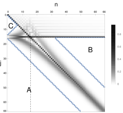
Figure 3.1. The magnitude plot of the Jacobi coefficients $\rho_{j,n}^{15;(2.5,1.5)}$.

We calculate the coefficients $\rho_{j,n}^{m;(\alpha,\beta)}$ with $\alpha=2.5$ and $\beta=1.5$ for $m=15$ using Theorem 3.4 and show their magnitudes for $0\leqslant j,n\leqslant 66$ in Figure 3.1. That is, the $n$-th column in this matrix plot corresponds to $\rho_{j,n}^{15;(2.5,1.5)}$. There are three regions of exact zeros which are indicated by solid lines. The coefficients $\rho_{j,n}^{15;(2.5,1.5)}$ are exact zeros in Region A simply because the convolution of $P_{15}^{(2.5,1.5)}$ and $P_{n}^{(2.5,1.5)}$ is a polynomial of degree $n+16$. The zeros in Region B correspond to (3.12b). Finally, we note that $m\geqslant 2n+3$ in Region C and by swapping the roles of $m$ and $n$ we see the exact zeros in Region C, again, from (3.12b).

In [12, Th. 4.8], it is shown that the coefficients $\rho_{j,n}^{m;(\alpha,\beta)}$ are symmetric up to a scaling for $j,n\geqslant m+1$:

(3.15) $$\rho_{n,j}^{m;(\alpha,\beta)}=(-1)^{j+n}\frac{(\alpha+\beta+2n+1)(\alpha+1)_{j}(\beta+1)_{j}\Big{(}(\alpha+\beta+1)_{n}\Big{)}^{2}}{(\alpha+\beta+2j+1)(\alpha+1)_{n}(\beta+1)_{n}\Big{(}(\alpha+\beta+1)_{j}\Big{)}^{2}}\rho_{j,n}^{m;(\alpha,\beta)},$$

which can be shown from (3.12d) with some tedious and lengthy work. However, this symmetry property is readily seen for the symmetric Jacobi case where $\alpha=\beta$ and we show this in the next subsection. In Figure 3.1, the entries that satisfy this symmetry property are those in the lower right part that is bordered by the dashed lines.

Bateman’s formula for the expansion of Jacobi polynomials with two variables is well known (see, for example, [4, Theorem 4.3.3]). In passing, we obtain the following proposition where we show the binomial-type tensor product expansion of $P_{m}^{(\alpha,\beta)}(x-t)$ in $P_{j}^{(\alpha,\beta)}(x+1)$ and $P_{k}^{(\alpha,\beta)}(t)$. This way, the variables $x$ and $t$ in a Jacobi-polynomial-based difference kernel [5, p. 37] become detached.

Proposition 3.5.

For the $m$-th degree Jacobi polynomial $P_{m}^{(\alpha,\beta)}(x)$,

(3.16) $$P_{m}^{(\alpha,\beta)}(x-t)=\sum_{k=0}^{m}\sum_{j=0}^{m-k}c_{m-k,j}^{m,(\alpha,\beta)}P_{j}^{(\alpha,\beta)}(x+1)P^{(\alpha,\beta)}_{k}(t),$$

where

(3.17) $$\begin{multlined}c_{m-k,j}^{m,(\alpha,\beta)}=\sum_{\nu=k}^{m-j}\frac{(-1)^{\nu}(\alpha+\beta+2k+1)}{(\beta+\nu+1)_{k-\nu}(\alpha+\beta+k+1)_{\nu+1}(\nu-k)!}\\ \hskip 85.35826pt\times\frac{(j+\nu+\alpha+1)_{m-\nu-j}(m+\alpha+\beta+1)_{\nu}(m+\nu+\alpha+\beta+1)_{j}}{(m-\nu-j)!(j+\alpha+\beta+1)_{j}}\\ \hskip 85.35826pt\times{}_{3}F_{2}\left({j-m+\nu,j+\alpha+1,j+m+\nu+\alpha+\beta+1\atop j+\nu+\alpha+1,2j+\alpha+\beta+2};1\right).\end{multlined}c_{m-k,j}^{m,(\alpha,\beta)}=\sum_{\nu=k}^{m-j}\frac{(-1)^{\nu}(\alpha+\beta+2k+1)}{(\beta+\nu+1)_{k-\nu}(\alpha+\beta+k+1)_{\nu+1}(\nu-k)!}\\ \hskip 85.35826pt\times\frac{(j+\nu+\alpha+1)_{m-\nu-j}(m+\alpha+\beta+1)_{\nu}(m+\nu+\alpha+\beta+1)_{j}}{(m-\nu-j)!(j+\alpha+\beta+1)_{j}}\\ \hskip 85.35826pt\times{}_{3}F_{2}\left({j-m+\nu,j+\alpha+1,j+m+\nu+\alpha+\beta+1\atop j+\nu+\alpha+1,2j+\alpha+\beta+2};1\right).$$

Proof.

By Taylor expansion of $P_{m}^{(\alpha,\beta)}(x-t)$ about $t=-1$, we have

$$P_{m}^{(\alpha,\beta)}(x-t)=\sum_{\nu=0}^{m}\frac{(-1)^{\nu}}{\nu!}\frac{\mathrm{d}^{\nu}P_{m}^{(\alpha,\beta)}(x+1)}{\mathrm{d}(x+1)^{\nu}}(t+1)^{\nu}.$$

Using (3.5) and (3.10), the latter equation becomes

$$P_{m}^{(\alpha,\beta)}(x-t)=\sum_{\nu=0}^{m}\frac{(-1)^{\nu}}{\nu!}\left(\sum_{j=0}^{m-\nu}\gamma_{m-\nu,j}^{(\nu,0)}(\alpha,\beta)P_{j}^{(\alpha,\beta)}(x+1)\right)\left(\sum_{k=0}^{\nu}b_{\nu,k}{(\alpha,\beta)}P_{k}^{(\alpha,\beta)}(t)\right).$$

We swap the order of the $k$- and the $\nu$-summations and then that of the $\nu$- and the $j$-summations to obtain (3.16) with

$$c_{m-k,j}^{m,(\alpha,\beta)}=\sum_{\nu=k}^{m-j}\frac{(-1)^{\nu}}{\nu!}b_{\nu,k}{(\alpha,\beta)}\gamma_{m-\nu,j}^{(\nu,0)}(\alpha,\beta).$$

Substituting in the expressions of $b_{\nu,k}{(\alpha,\beta)}$ and $\gamma_{m-\nu,j}^{(\nu,0)}(\alpha,\beta)$, given by (3.11) and (3.6) respectively, leads to (3.17). ∎

3.2. Symmetric Jacobi polynomials

In this subsection, we give in Corollary 3.7 the convolution coefficients $\rho_{k,n}^{m;(\alpha,\beta)}$ for the Jacobi polynomials with $\alpha=\beta$. These coefficients could be obtained from Theorem 3.4 by simply setting $\beta=\alpha$. However, a lengthy simplification is necessary in order to obtain exactly what is given in Corollary 3.7. The route we take is to obtain the explicit expressions for $\gamma_{n,k}^{(p,q)}(\alpha,\alpha)$, $b_{n,k}(\alpha,\alpha)$, and $\left.\frac{\mathrm{d}^{p}}{\mathrm{d}x^{p}}P_{n}^{(\alpha,\alpha)}(x)\right|_{x=-1}$, from which we derive $\varpi_{j,\nu}^{m,n}(\alpha,\alpha)$ and $d_{\nu,j,n}^{m}(\alpha,\alpha)$ using (3.13).

Lemma 3.6.

When $n-k$ is even,

(3.18a) $$\gamma_{n,k}^{(p,q)}(\alpha,\alpha)=\displaystyle\frac{\left(p-q\right)_{\frac{n-k}{2}}(\alpha+k+q+\frac{1}{2})\Gamma(k+q+2\alpha+1)\Gamma(n+p+\alpha+1)\Gamma\left(\frac{k+n+1}{2}+p+\alpha\right)}{2^{q-p}\left(\frac{n-k}{2}\right)!\Gamma(k+q+\alpha+1)\Gamma(n+p+2\alpha+1)\Gamma\left(\frac{k+n+3}{2}+q+\alpha\right)},$$

and

(3.18b) $$\gamma_{n,k}^{(p,q)}(\alpha,\alpha)=0$$

otherwise.

Proof.

The connection coefficients in (3.7) with $\beta=\alpha$ and $\delta=\gamma$ can be found in [1, Theorem 7.1.4]:

(3.19) $$a_{n,k}^{(\alpha+p,\alpha+p;\alpha+q,\alpha+q)}=\frac{(p-q)_{\frac{n-k}{2}}\left(q+\alpha+\frac{3}{2}\right)_{k}(2(q+\alpha)+1)_{k}(p+\alpha+1)_{n}\left(p+\alpha+\frac{1}{2}\right)_{\frac{k+n}{2}}}{\left(\frac{n-k}{2}\right)!\left(q+\alpha+\frac{1}{2}\right)_{k}(q+\alpha+1)_{k}(2(p+\alpha)+1)_{n}\left(q+\alpha+\frac{3}{2}\right)_{\frac{k+n}{2}}},$$

when $n-k$ is even, while

$$a_{n,k}^{(\alpha+p,\alpha+p;\alpha+q,\alpha+q)}=0,$$

when $n-k$ is odd, implied by $P_{n}^{(\alpha,\alpha)}(-x)=(-1)^{n}P_{n}^{(\alpha,\alpha)}(x)$ [1, Theorem 7.1.4]. Now the relation (3.9) between the $a$- and the $\gamma$-coefficients readily show that $\gamma_{n,k}^{(p,q)}(\alpha,\alpha)=0$ when $n-k$ is odd. For the case where $n-k$ is even, we substitute (3.19) in (3.9) and simplify using the Legendre duplication formula [8, Eq. (5.5.5)] to obtain (3.18). ∎

Corollary 3.7.

Let $m$ and $n$ be two positive integers with $n\geqslant m$ and suppose $\alpha>-1$ to be nonzero. For $\alpha=\beta$, the $\rho$-coefficients in the expansion (3.1) become

(3.20a) $$\rho_{j,n}^{m;(\alpha,\alpha)} =\sum_{\nu=\max(1,|j-n|)}^{m+1}\varpi_{j,\nu}^{m,n}(\alpha,\alpha) \quad\text{ for }j\geqslant\max(m+1,n-m-1),$$

(3.20b) $$\rho_{j,n}^{m;(\alpha,\alpha)} =0 \quad\text{ for }m+1\leqslant j\leqslant n-m-2,\text{ if }n\geqslant 2m+3,$$

(3.20c) $$\rho_{j,n}^{m;(\alpha,\alpha)} =\sum_{\nu=1}^{j}\varpi_{j,\nu}^{n,m}(\alpha,\alpha)+\sum_{\nu=j+1}^{n+1}d_{\nu,j,n}^{m}(\alpha,\alpha) \quad\text{ for }0\leqslant j\leqslant m,$$

where

(3.20d) $$\begin{multlined}\varpi_{j,\nu}^{m,n}(\alpha,\alpha)=\frac{2(-1)^{m+\nu+1}(\alpha+\nu)_{m+1-\nu}(m+2\alpha+1)_{\nu-1}(n+2\alpha+1)_{j-\nu}}{(m-\nu+1)!\left(\frac{n+\nu-j}{2}\right)!}\\ \times\frac{(-\nu)_{\frac{n+\nu-j}{2}}\left(j+\alpha-\nu+\frac{1}{2}\right)_{\frac{n+\nu-j}{2}}(j+\alpha-\nu+1)_{n+\nu-j}}{(j+2\alpha+1)_{j}\left(j+\alpha+\frac{3}{2}\right)_{\frac{n+\nu-j}{2}}(2j+2\alpha-2\nu+1)_{n+\nu-j}}\end{multlined}\varpi_{j,\nu}^{m,n}(\alpha,\alpha)=\frac{2(-1)^{m+\nu+1}(\alpha+\nu)_{m+1-\nu}(m+2\alpha+1)_{\nu-1}(n+2\alpha+1)_{j-\nu}}{(m-\nu+1)!\left(\frac{n+\nu-j}{2}\right)!}\\ \times\frac{(-\nu)_{\frac{n+\nu-j}{2}}\left(j+\alpha-\nu+\frac{1}{2}\right)_{\frac{n+\nu-j}{2}}(j+\alpha-\nu+1)_{n+\nu-j}}{(j+2\alpha+1)_{j}\left(j+\alpha+\frac{3}{2}\right)_{\frac{n+\nu-j}{2}}(2j+2\alpha-2\nu+1)_{n+\nu-j}}$$

when $$n+\nu-j$$ is even and

(3.20e) $$\varpi_{j,\nu}^{m,n}(\alpha,\alpha)=0$$

otherwise. Here,

(3.20f) $$\begin{multlined}d_{\nu,j,n}^{m}(\alpha,\alpha)=\frac{2(-1)^{m+n+1+\nu}(2\alpha+2j+1)(\alpha+\nu)(j+\alpha+1)_{m-j}(\alpha+1)_{n}(n+1+2\alpha)_{\nu-1}}{m!(n+1-\nu)!(\nu-j)!(j+2\alpha+1)_{\nu+1}}\\[5.69054pt] \times{}_{4}F_{3}\left({1,-m,\alpha+\nu+1,m+2\alpha+1\atop\nu-j+1,\alpha+1,j+2\alpha+\nu+2};1\right).\end{multlined}d_{\nu,j,n}^{m}(\alpha,\alpha)=\frac{2(-1)^{m+n+1+\nu}(2\alpha+2j+1)(\alpha+\nu)(j+\alpha+1)_{m-j}(\alpha+1)_{n}(n+1+2\alpha)_{\nu-1}}{m!(n+1-\nu)!(\nu-j)!(j+2\alpha+1)_{\nu+1}}\\[5.69054pt] \times{}_{4}F_{3}\left({1,-m,\alpha+\nu+1,m+2\alpha+1\atop\nu-j+1,\alpha+1,j+2\alpha+\nu+2};1\right).$$

Proof.

The $\rho$-coefficients in (3.20) inherit from (3.12).

From (3.4), we have

(3.21) $$\left.\frac{\mathrm{d}^{p}}{\mathrm{d}x^{p}}P_{n}^{(\alpha,\alpha)}(x)\right|_{x=-1}=\frac{2^{-p}(-1)^{n+p}(p+\alpha+1)_{n-p}(n+2\alpha+1)_{p}}{(n-p)!}.$$

Substituting (3.18) and (3.21) into (3.13a), we have (3.20d) and (3.20e) after some algebraic simplifications.

Replacing $\beta$ by $\alpha$ in (3.12e) gives (3.20f). ∎

The following proposition instantiates the symmetry property for the symmetric Jacobi-based coefficients, which can be easily derived from Corollary 3.7.

Proposition 3.8.

For $j,n\geqslant m+1$, the $\rho$-coefficients in (3.1) with $\beta=\alpha$ satisfy

(3.22) $$\rho_{j,n}^{m;(\alpha,\alpha)}=(-1)^{j+n}\frac{(2\alpha+2j+1)\left((2\alpha+1)_{j}\right)^{2}\left((\alpha+1)_{n}\right)^{2}}{(2\alpha+2n+1)\left((\alpha+1)_{j}\right)^{2}\left((2\alpha+1)_{n}\right)^{2}}\rho_{n,j}^{m;(\alpha,\alpha)}.$$

Proof.

When $(n+\nu-j)$ is even, so is $(j+\nu-n)$ and (3.20d) gives

(3.23) $$\frac{\varpi_{j,\nu}^{m,n}(\alpha,\alpha)}{\varpi_{n,\nu}^{m,j}(\alpha,\alpha)}=(-1)^{j+n}\frac{(2\alpha+2j+1)\left((2\alpha+1)_{j}\right)^{2}\left((\alpha+1)_{n}\right)^{2}}{(2\alpha+2n+1)\left((\alpha+1)_{j}\right)^{2}\left((2\alpha+1)_{n}\right)^{2}},$$

which is independent from $\nu$. If $|n-j|\leqslant m+1$, (3.23) and (3.20a) imply (3.22).

If $n\geqslant 2m+3$, for $m+1\leqslant j\leqslant n-m-2$ we have $\rho_{j,n}^{m;(\alpha,\alpha)}=0$, as indicated by (3.20b). Also, $j\leqslant n-m-2$ suggests $n\geqslant j+m+2$, in which case $\rho_{n,j}^{m;(\alpha,\alpha)}=0$. Therefore, (3.22) holds too for $m+1\leqslant j\leqslant n-m-2$.

Hence, (3.22) is true for $j,n\geqslant m+1$. ∎

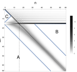
Figure 3.2. The magnitude plot of the symmetric Jacobi coefficients $\rho_{j,n}^{15;(2.5,2.5)}$.

Figure 3.2 shows the magnitudes of the coefficients $\rho_{j,n}^{m;(\alpha,\alpha)}$ with $\alpha=2.5$ and $m=15$. The regions A, B, and C with exact zeros are inherited from those of the Jacobi-based convolution coefficients. The symmetric coefficients are bordered by the dashed lines.

3.2.1. Gegenbauer case

Gegenbauer polynomials $C_{n}^{(\lambda)}$ are symmetric Jacobi polynomials with a different normalization:

(3.24) $$C_{n}^{(\lambda)}(x)=\frac{\left(2\lambda\right)_{n}}{\left(\lambda+\frac{1}{2}\right)_{n}}P_{n}^{(\lambda-\frac{1}{2},\lambda-\frac{1}{2})}(x),\ n\geqslant 0,$$

with $\lambda>-\frac{1}{2}$ and $\lambda\neq 0$. If we denote by $\widetilde{\rho}_{k,n}^{m;(\lambda)}$ the series coefficients of the convolution of two Gegenbauer polynomials, that is,

(3.25) $$\int_{-1}^{x+1}C_{m}^{(\lambda)}(x-t)C_{n}^{(\lambda)}(t)\mathrm{d}t=\sum_{k=0}^{m+n+1}\widetilde{\rho}_{j,n}^{m;(\lambda)}C_{j}^{(\lambda)}(x+1),$$

the relation (3.24) gives

(3.26) $$\widetilde{\rho}_{j,n}^{m;(\lambda)}=\frac{\left(\lambda+\frac{1}{2}\right)_{j}(2\lambda)_{m}(2\lambda)_{n}}{(2\lambda)_{j}\left(\lambda+\frac{1}{2}\right)_{m}\left(\lambda+\frac{1}{2}\right)_{n}}\rho_{j,n}^{m;(\lambda-1/2;\lambda-1/2)},$$

where $\rho_{j,n}^{m;(\lambda-1/2;\lambda-1/2)}$ are the coefficients given in Corollary 3.7. Combining Corollary 3.7 and (3.26) leads to the following corollary, the proof of which is omitted.

Corollary 3.9.

Let $m$ and $n$ be two positive integers with $n\geqslant m$ and suppose $\lambda>-\frac{1}{2}$ to be nonzero. The $\widetilde{\rho}$-coefficients in the expansion (3.25) can be expressed as

$$\widetilde{\rho}_{j,n}^{m;(\lambda)} =\sum_{\nu=\max(1,|j-n|)}^{m+1}\widetilde{\varpi}_{j,\nu}^{m,n}(\lambda) \quad\text{ for }j\geqslant\max(m+1,n-m-1),$$

$$\widetilde{\rho}_{j,n}^{m;(\lambda)} =0 \quad\text{ for }m+1\leqslant j\leqslant n-m-2,\text{ if }n\geqslant 2m+3,$$

$$\widetilde{\rho}_{j,n}^{m;(\lambda)} =\sum_{\nu=1}^{j}\widetilde{\varpi}_{j,\nu}^{n,m}(\lambda)+\sum_{\nu=j+1}^{n+1}\widetilde{d}_{\nu,j,n}^{m}(\lambda) \quad\text{ for }0\leqslant j\leqslant m,$$

where

$$\widetilde{\varpi}_{j,\nu}^{m,n}(\lambda)=\frac{(j+\lambda)(-1)^{m+\nu+1}(\lambda)_{\nu-1}(2\lambda+2\nu-2)_{m-\nu+1}(-\nu)_{\frac{-j+n+\nu}{2}}}{2(m-\nu+1)!\left(\frac{-j+\nu+n}{2}\right)!\left(\lambda+\frac{j+n-\nu}{2}\right)_{\nu+1}}$$

when $n+\nu-j$ is even and $\widetilde{\varpi}_{j,\nu}^{m,n}(\lambda)=0$ otherwise. Here,

$$\begin{multlined}\widetilde{d}_{\nu,j,n}^{m}(\lambda)=\frac{2(-1)^{m+\nu+n+1}(j+\lambda)(2\lambda+2\nu-1)(2\lambda)_{m}(j+2\lambda+\nu+1)_{-j+n-2}}{m!(\nu-j)!(-\nu+n+1)!}\\[5.69054pt] \times{}_{4}F_{3}\left({1,-m,m+2\lambda,\lambda+\nu+\frac{1}{2}\atop\lambda+\frac{1}{2},-j+\nu+1,j+2\lambda+\nu+1};1\right).\end{multlined}\widetilde{d}_{\nu,j,n}^{m}(\lambda)=\frac{2(-1)^{m+\nu+n+1}(j+\lambda)(2\lambda+2\nu-1)(2\lambda)_{m}(j+2\lambda+\nu+1)_{-j+n-2}}{m!(\nu-j)!(-\nu+n+1)!}\\[5.69054pt] \times{}_{4}F_{3}\left({1,-m,m+2\lambda,\lambda+\nu+\frac{1}{2}\atop\lambda+\frac{1}{2},-j+\nu+1,j+2\lambda+\nu+1};1\right).$$

3.2.2. Legendre case

Legendre polynomials $P_{n}^{(0,0)}(x)$ are the symmetric Jacobi polynomials with $\alpha=\beta=0$ or, equivalently, the special case of Gegenbauer polynomials with $\lambda=1/2$. We show in the following corollary that the convolution coefficients of Legendre polynomials become significantly simpler than those of symmetric Jacobi or Gegenbauer.

Corollary 3.10.

Let $m$ and $n$ be two positive integers with $n\geqslant m$. The coefficients $\rho_{j,n}^{m;(0,0)}$ in (3.1) can be expressed as

$$\rho_{j,n}^{m;(0,0)} =\sum_{\nu=\max(1,|j-n|)}^{m+1}\varpi_{j,\nu}^{m,n}(0,0) \quad\text{ for }j\geqslant\max(m+1,n-m-1),$$

$$\rho_{j,n}^{m;(0,0)} =0 \quad\text{ for }m+1\leqslant j\leqslant n-m-2,\text{ if }n\geqslant 2m+3,$$

$$\rho_{j,n}^{m;(0,0)} =\sum_{\nu=1}^{j}\varpi_{j,\nu}^{n,m}(0,0)+\sum_{\nu=j+1}^{n+1}d_{\nu,j,n}^{m} \quad\text{ for }0\leqslant j\leqslant m,$$

where

(3.27a) $$\varpi_{j,\nu}^{m,n}(0,0)=\frac{(-1)^{m+\nu+1}(2j+1)(m+\nu-1)!(-\nu)_{\frac{n-j+\nu}{2}}}{4^{\nu}(\nu-1)!(m-\nu+1)!\left(\frac{n-j+\nu}{2}\right)!\left(\frac{n+j-\nu+1}{2}\right)_{\nu+1}}$$

for even $$n+\nu-j \varpi_{j,\nu}^{m,n}(0,0)=0$$ and otherwise. Here,

(3.27b) $${d}_{\nu,j,n}^{m}(0,0)=\frac{\sqrt{\pi}(2j+1)\nu 2^{j+m-\nu}(-1)^{m+\nu+n+1}(n+\nu-1)!\left(\frac{-j-m+\nu+1}{2}\right)_{j+m}\left(\frac{j-m+\nu+2}{2}\right)_{m}}{(n-\nu+1)!(j+m+\nu)!\Gamma\left(\frac{-j+m+\nu+2}{2}\right)\Gamma\left(\frac{j+m+\nu+3}{2}\right)}.$$

Proof.

Since $P_{n}(x)=P_{n}^{(0,0)}(x)$, (3.27a) can be obtained by setting $\alpha=0$ in (3.20d) and simplifying using the Legendre duplication formula.

Setting $\alpha=0$ in (3.20f), we have

$${d}_{\nu,j,n}^{m}(0,0)=\frac{2(-1)^{\nu+m+n+1}v(2j+1)(n+\nu-1)!}{(n-\nu+1)!(\nu-j)!(j+\nu+1)!}{}_{3}F_{2}\left({-m,m+1,\nu+1\atop-j+\nu+1,j+\nu+2};1\right),$$

where the generalized hypergeometric series ${}_{3}F_{2}$ can be represented in terms of Gamma functions using the Whipple’s sum [8, Eq. (16.4.7)]. Further algebraic simplification using the Legendre duplication formula gives (3.27b). ∎

The following theorem shows that the symmetry property (3.15) holds for all $j,n\geqslant 0$ in the Legendre case, which is difficult to see directly from Theorem 3.10. Our proof employs the fact that the Legendre polynomials are $L^{2}$ orthogonal on $[-1,1]$.

Theorem 3.11.

For any $m,n,j\geqslant 0$, the coefficients $\rho_{j,n}^{m;(0,0)}$ in (3.1) satisfy

(3.28) $$\rho_{j,n}^{m;(0,0)}=(-1)^{n+j}\frac{2j+1}{2n+1}\rho_{n,j}^{m;(0,0)}.$$

Proof.

As indicated in (1.2), $x\in[-2,0]$ in (3.1). By letting $y=x+1$, we have

$$\int_{-1}^{y}P_{m}^{(0,0)}(y-t-1)P_{n}^{(0,0)}(t)\mathrm{d}t=\sum_{k=0}^{m+n+1}\rho_{k,n}^{m;(0,0)}P_{k}^{(0,0)}(y),$$

where $y\in[-1,1]$. Since the Legendre polynomials are $L^{2}$ orthogonal, i.e. for $j,n\geqslant 0$,

$$\int_{-1}^{1}P^{(0,0)}_{j}(y)P^{(0,0)}_{k}(y)\mathrm{d}y=\frac{2}{2j+1}\delta_{j,k},$$

we have

(3.29) $$\int_{-1}^{1}P^{(0,0)}_{j}(y)\int_{-1}^{y}P^{(0,0)}_{m}(y-t-1)P^{(0,0)}_{n}(t)\mathrm{d}t\mathrm{d}y=\frac{2}{2j+1}\rho_{j,n}^{m;(0,0)}$$

for $0\leqslant j\leqslant m+n+1$.

Now, we swap the order of integration to have

$$\int_{-1}^{1}P^{(0,0)}_{j}(y)\int_{-1}^{y}P^{(0,0)}_{m}(y-t-1)P^{(0,0)}_{n}(t)\mathrm{d}t\mathrm{d}y=\int_{-1}^{1}P^{(0,0)}_{n}(t)\int_{t}^{1}P^{(0,0)}_{j}(y)P^{(0,0)}_{m}(y-t-1)\mathrm{d}y\mathrm{d}t,$$

where $t\in[-1,1]$. Applying the changes of variables $t=-T$ and $y=-Y$ gives

(3.30) $$\begin{multlined}\int_{-1}^{1}P^{(0,0)}_{j}(y)\int_{-1}^{y}P^{(0,0)}_{m}(y-t-1)P^{(0,0)}_{n}(t)\mathrm{d}t\mathrm{d}y\\ \hskip 113.81102pt=(-1)^{n+j}\int_{-1}^{1}P^{(0,0)}_{n}(T)\int_{-1}^{T}P^{(0,0)}_{j}(Y)P^{(0,0)}_{m}(T-Y-1)\mathrm{d}Y\mathrm{d}T,\end{multlined}\int_{-1}^{1}P^{(0,0)}_{j}(y)\int_{-1}^{y}P^{(0,0)}_{m}(y-t-1)P^{(0,0)}_{n}(t)\mathrm{d}t\mathrm{d}y\\ \hskip 113.81102pt=(-1)^{n+j}\int_{-1}^{1}P^{(0,0)}_{n}(T)\int_{-1}^{T}P^{(0,0)}_{j}(Y)P^{(0,0)}_{m}(T-Y-1)\mathrm{d}Y\mathrm{d}T,$$

where we have used $P_{n}(y)=(-1)^{n}P_{n}(-y)$.

Recognizing the inner integral in (3.30) as the convolution of $P_{j}(T)$ and $P_{m}(T)$ with $T\in[-1,1]$, we can replace it by its series representation

(3.31) $$\begin{multlined}\int_{-1}^{1}P^{(0,0)}_{j}(y)\int_{-1}^{y}P^{(0,0)}_{m}(y-t-1)P^{(0,0)}_{n}(t)\mathrm{d}t\mathrm{d}y\\ \hskip 56.9055pt=(-1)^{n+j}\sum_{k=0}^{j+m+1}\rho_{k,j}^{m;(0,0)}\int_{-1}^{1}P^{(0,0)}_{n}(T)P^{(0,0)}_{k}(T)\mathrm{d}T=(-1)^{n+j}\frac{2}{2n+1}\rho_{n,j}^{m;(0,0)},\end{multlined}\int_{-1}^{1}P^{(0,0)}_{j}(y)\int_{-1}^{y}P^{(0,0)}_{m}(y-t-1)P^{(0,0)}_{n}(t)\mathrm{d}t\mathrm{d}y\\ \hskip 56.9055pt=(-1)^{n+j}\sum_{k=0}^{j+m+1}\rho_{k,j}^{m;(0,0)}\int_{-1}^{1}P^{(0,0)}_{n}(T)P^{(0,0)}_{k}(T)\mathrm{d}T=(-1)^{n+j}\frac{2}{2n+1}\rho_{n,j}^{m;(0,0)},$$

where the second equality follows from the orthogonality. Finally, (3.29) and (3.31) leads to (3.28). ∎

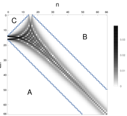
Figure 3.3. The magnitude plot of the Legendre coefficients $\rho_{j,n}^{15;(0,0)}$.

The Legendre-based symmetry property (3.28) suggests extended regions of exact zeros in the magnitude plot, as seen in Figure 3.3. Now, the non-zero coefficients are confined in a tilted rectangle-shaped band surrounded by zeros in Regions A, B, and C.

3.2.3. Chebyshev case

Chebyshev polynomials of second kind $T_{n}(x)$ are symmetric Jacobi polynomials with $\alpha=\beta=-1/2$ and a different normalization:

(3.32) $$P_{n}^{(-1/2,-1/2)}(x)=\frac{\left(1/2\right)_{n}}{n!}T_{n}(x),\ n\geqslant 0.$$

Corollary 3.12.

Let $m$ and $n$ be two positive integers with $n\geqslant m$. The coefficients $\widetilde{\rho}_{k,n}^{m}$ in the expansion

$$\int_{-1}^{x+1}T_{m}(x-t)T_{n}(t)\mathrm{d}t=\sum_{k=0}^{m+n+1}\widetilde{\rho}_{k,n}^{m}T_{k}(x+1),$$

can be expressed as

(3.33a) $$\widetilde{\rho}_{j,n}^{m} =\sum_{\nu=\max(1,|j-n|)}^{m+1}\widetilde{\varpi}_{j,\nu}^{m,n} \quad\text{ for }j\geqslant\max(m+1,n-m-1),$$

(3.33b) $$\widetilde{\rho}_{j,n}^{m} =0 \quad\text{ for }m+1\leqslant j\leqslant n-m-2,\text{ if }n\geqslant 2m+3,$$

(3.33c) $$\widetilde{\rho}_{j,n}^{m} =\sum_{\nu=1}^{j}\widetilde{\varpi}_{j,\nu}^{n,m}+\sum_{\nu=j+1}^{n+1}\widetilde{d}_{\nu,j,n}^{m} \quad\text{ for }0\leqslant j\leqslant m,$$

where

(3.33d) $$\widetilde{\varpi}_{j,\nu}^{m,n}=\frac{(-1)^{m}\,2^{1-2\nu}n(-m)_{\nu-1}(m)_{\nu-1}(-\nu)_{\frac{n+\nu-j}{2}}\left(\frac{n+\nu-j+2}{2}\right)_{j-\nu-1}}{\left(1/2\right)_{\nu-1}\left(\frac{n+\nu+j}{2}\right)!}$$

for even $$(n+\nu-j) \widetilde{\varpi}_{j,\nu}^{m,n}=0$$ and otherwise. Here,

(3.33e) $$\widetilde{d}_{\nu,j,n}^{\ m}=\frac{2^{2-\delta_{0,j}}(-1)^{m+n}(-n)_{\nu-1}(n)_{\nu-1}\left(\nu-1/2\right)}{(\nu-j)!(j+\nu)!}{}_{4}F_{3}\left({1,-m,m,\nu+1/2\atop 1/2,-j+\nu+1,j+\nu+1};1\right).$$

Proof.

Equation (3.32) suggests

(3.34) $$\widetilde{\rho}_{j,n}^{m}=\frac{m!n!(1/2)_{j}}{(1/2)_{m}(1/2)_{n}j!}\rho_{j,n}^{m;(-1/2,-1/2)},$$

which leads to (3.33a)-(3.33c) with

$$\widetilde{\varpi}_{j,\nu}^{m,n}=\frac{m!n!(1/2)_{j}}{(1/2)_{m}(1/2)_{n}j!}\varpi_{j,\nu}^{m,n}(-1/2,-1/2).$$

Setting $\alpha=-1/2$ in (3.20d) and simplifying give (3.33d).

Similarly, (3.34) implies

(3.35) $$\widetilde{d}_{\nu,j,n}^{\ m}=\frac{m!n!(1/2)_{j}}{(1/2)_{m}(1/2)_{n}j!}d_{\nu,j,n}^{m}(-1/2,-1/2),$$

where

(3.36) $$\begin{multlined}d_{\nu,j,n}^{m}(-1/2,-1/2)=\frac{4(-1)^{m+n+1+\nu}(-1/2+\nu)(j+1/2)_{m-j}(1/2)_{n}(n)_{\nu-1}}{m!(n+1-\nu)!(\nu-j)!(j+1)_{\nu}}\\[5.69054pt] \times{}_{4}F_{3}\left({1,-m,1/2+\nu,m\atop\nu-j+1,1/2,j+\nu+1};1\right)\end{multlined}d_{\nu,j,n}^{m}(-1/2,-1/2)=\frac{4(-1)^{m+n+1+\nu}(-1/2+\nu)(j+1/2)_{m-j}(1/2)_{n}(n)_{\nu-1}}{m!(n+1-\nu)!(\nu-j)!(j+1)_{\nu}}\\[5.69054pt] \times{}_{4}F_{3}\left({1,-m,1/2+\nu,m\atop\nu-j+1,1/2,j+\nu+1};1\right)$$

for $j\geqslant 1$. When $j=0$, (3.20f) gives

$$d_{\nu,0,n}^{m}(-1/2,-1/2)= \lim_{\alpha\to-1/2}d_{\nu,0,n}^{m}(\alpha,\alpha)$$

(3.37) $$= \frac{2(-1)^{m+n+1+\nu}(\nu-1/2)(1/2)_{m}(1/2)_{n}(n)_{\nu-1}}{m!(n+1-\nu)!(\nu!)^{2}}{}_{4}F_{3}\left({1,-m,1/2+\nu,m\atop\nu+1,1/2,\nu+1};1\right).$$

By combining (3.36) and (3.37), we have

$$\begin{multlined}d_{\nu,j,n}^{m}(-1/2,-1/2)=\frac{2^{2-\delta_{0,j}}(-1)^{m+n+1+\nu}(-1/2+\nu)(j+1/2)_{m-j}(1/2)_{n}(n)_{\nu-1}}{m!(n+1-\nu)!(\nu-j)!(j+1)_{\nu}}\\[5.69054pt] \times{}_{4}F_{3}\left({1,-m,1/2+\nu,m\atop\nu-j+1,1/2,j+\nu+1};1\right),\end{multlined}d_{\nu,j,n}^{m}(-1/2,-1/2)=\frac{2^{2-\delta_{0,j}}(-1)^{m+n+1+\nu}(-1/2+\nu)(j+1/2)_{m-j}(1/2)_{n}(n)_{\nu-1}}{m!(n+1-\nu)!(\nu-j)!(j+1)_{\nu}}\\[5.69054pt] \times{}_{4}F_{3}\left({1,-m,1/2+\nu,m\atop\nu-j+1,1/2,j+\nu+1};1\right),$$

which, along with (3.35), yields (3.33e). ∎

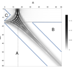
Figure 3.4. The magnitude plot of the Chebyshev coefficients $\widetilde{\rho}_{j,n}^{15}$.

Figure 3.4 shows the magnitudes of the coefficients $\rho_{j,n}^{m}$ for $m=15$ and the region A, B, and C where $\rho_{j,n}^{m}$ are exactly zero. The coefficients that satisfy the symmetry are encompassed by the dashed lines.

4. Laguerre case

Laguerre polynomials parameterized by $\alpha$ with $\Re(\alpha)>-1$ can be defined in terms of terminating hypergeometric functions with the following commonly-used normalization

$$L_{n}^{(\alpha)}(x)=\frac{(1+\alpha)_{n}}{n!}{}_{1}F_{1}\left({-n\atop\alpha+1};x\right),~{}~{}~{}~{}~{}~{}n\geqslant 0,$$

and they satisfy the orthogonality relations

$$\int_{0}^{+\infty}x^{\alpha}\text{e}^{-x}L_{k}^{(\alpha)}(x)L_{n}^{(\alpha)}(x)\mathrm{d}x=\frac{\Gamma(\alpha+n+1)}{n!}\delta_{n,k}.$$

Laguerre polynomials with different parameters are linearly related via [2, (3.46)]

(4.1) $$L_{n}^{(\alpha)}(x)=\sum_{k=0}^{n}\frac{(\alpha-\beta)_{n-k}}{(n-k)!}L_{k}^{(\beta)}(x),$$

and the $p$-th derivatives of $L_{n+p}^{(\alpha)}$ equals to $L_{n}^{(\alpha+p)}$ up to a sign:

(4.2) $$\frac{\mathrm{d}^{p}}{\mathrm{d}x^{p}}L_{n+p}^{(\alpha)}(x)=(-1)^{p}L_{n}^{(\alpha+p)}(x).$$

We combine (4.1) and (4.2) to have

(4.3) $$\frac{\mathrm{d}^{p}}{\mathrm{d}x^{p}}L_{n+p}^{(\alpha)}(x)=\sum_{k=0}^{n}\gamma_{n,k}^{(p,q)}(\alpha;L)\frac{\mathrm{d}^{q}}{\mathrm{d}x^{q}}L_{k+q}^{(\alpha)}(x),~{}~{}~{}\text{ where }~{}~{}~{}\gamma_{n,k}^{(p,q)}(\alpha;L)=\frac{(-1)^{p+q}(p-q)_{n-k}}{(n-k)!}.$$

The Laguerre representation of monomials can be found in, for example, [9, p.207]:

(4.4) $$x^{n}=\sum_{k=0}^{n}b_{n,k}(\alpha)L_{k}^{(\alpha)}(x),~{}~{}~{}\text{ where }~{}~{}~{}b_{n,k}{(\alpha)}=\frac{(-n)_{k}\Gamma(n+\alpha+1)}{\Gamma(k+\alpha+1)}=(-1)^{k}n!\left.\frac{\mathrm{d}^{k}{L_{n}^{(\alpha)}}}{\mathrm{d}x^{k}}\right|_{x=0}.$$

It also follows from (4.2) the value of $L_{n}^{(\alpha)}(x)$ or that of its derivatives at $x=0$:

(4.5) $$\left.\frac{\mathrm{d}^{p}{L_{n}^{(\alpha)}}}{\mathrm{d}x^{p}}\right|_{x=0}=(-1)^{p}\frac{(1+\alpha+p)_{n-p}}{(n-p)!}.$$

The Chu-Vandermonde’s identity used repeatedly in the rest of this section:

(4.6) $$\frac{(\alpha+\beta+2)_{n}}{n!}=\sum_{k=0}^{n}\frac{(\alpha+1)_{k}}{k!}\frac{(\beta+1)_{n-k}}{(n-k)!},$$

is valid for any complex numbers $\alpha$ and $\beta$. Observe that for $\alpha,\beta>-1$, it corresponds to (4.1) evaluated at $x=0$.

For the case of $\alpha=0$, convolution of Laguerre polynomials $L_{n}^{(0)}(x)$ and $L_{m}^{(0)}(x)$ is sparse in the sense that only two coefficients of its $L_{n}^{(0)}$-series representation are nonzero:

(4.7) $$\int_{0}^{x}L_{m}^{(0)}(x-t)L_{n}^{(0)}(t)\mathrm{d}t=-L_{m+n+1}^{(0)}(x)+L_{m+n}^{(0)}(x).$$

This well-known result can be found in, for example, [8, Eq. (18.17.2)] or [3, Eq. (7.411.4)]. There does not seem to be any similar formula addressing the cases with other values of $\alpha$ and this is what we present in Theorem 4.1 below.

Theorem 4.1.

Let $m$ and $n$ be two positive integers with $n\geqslant m$ and $\alpha$ be a complex number with $\Re(\alpha)>-1$. When $n\geqslant m+1$, the $\widehat{\rho}$-coefficients in the expansion

$$\int_{0}^{x}L_{m}^{(\alpha)}(x-t)L_{n}^{(\alpha)}(t)\mathrm{d}t=\sum_{j=0}^{m+n+1}\widehat{\rho}_{j,n}^{m;(\alpha)}L_{j}^{(\alpha)}(x)$$

are given by

(4.8a) $$-\frac{(\alpha-1)_{m+n+1-j}}{(m+n+1-j)!}\hskip 56.9055pt \text{for }n+1\leqslant j\leqslant m+n+1,$$

(4.8b) $$\frac{(\alpha)_{m}}{m!} \text{for }j=n,$$

(4.8c) $$\ 0 \text{for }m+1\leqslant j\leqslant n-1\hskip 14.22636pt\mbox{ (when }n\geqslant m+2\mbox{)},$$

(4.8d) $$\frac{(\alpha)_{n+1}}{(n+1)!} \text{for }j=m,$$

(4.8e) $$\frac{(\alpha-1)_{m+n+1-j}}{(m+n+1-j)!} \text{for }0\leqslant j\leqslant m-1.$$

In case of $n=m$, the $\widehat{\rho}$-coefficients become

(4.9a) $$-\frac{(\alpha-1)_{2m+1-j}}{(2m+1-j)!}\hskip 85.35826pt \text{for }m+1\leqslant j\leqslant 2m+1,$$

(4.9b) $$\frac{(\alpha)_{m+1}}{(m+1)!}+\frac{(\alpha)_{m}}{m!} \text{for }j=m,$$

(4.9c) $$\frac{(\alpha-1)_{2m+1-j}}{(2m+1-j)!} \text{for }0\leqslant j\leqslant m-1.$$

Proof.

With $a=0$, Theorem 2.3 gives

(4.10a) $$\widehat{\rho}_{j,n}^{m;(\alpha)}=\sum_{\nu=\max(1,j-n)}^{m+1}\gamma_{n-j+\nu,0}^{(j-\nu,j)}\left.\frac{\mathrm{d}^{\nu-1}{L_{m}^{(\alpha)}}}{\mathrm{d}x^{\nu-1}}\right|_{x=0}~{}~{}~{}~{}\text{ for }j\geqslant m+1$$

and

(4.10b) $$\begin{multlined}\widehat{\rho}_{j,n}^{m;(\alpha)}=\sum\limits_{\nu=1}^{j}\gamma_{m-j+\nu,0}^{(j-\nu,j)}\left.\frac{\mathrm{d}^{\nu-1}{L_{n}^{(\alpha)}}}{\mathrm{d}x^{\nu-1}}\right|_{x=0}\\ \hskip 28.45274pt+\sum\limits_{\nu=j+1}^{n+1}\left(\left.\frac{\mathrm{d}^{\nu-1}{L_{n}^{(\alpha)}}}{\mathrm{d}x^{\nu-1}}\right|_{x=0}\sum\limits_{p=0}^{m}\frac{b_{p+\nu,j}}{(p+\nu)!}\left.\frac{\mathrm{d}^{p}{L_{m}^{(\alpha)}}}{\mathrm{d}x^{p}}\right|_{x=0}\right)~{}~{}~{}~{}\text{ for }0\leqslant j\leqslant m,\end{multlined}\widehat{\rho}_{j,n}^{m;(\alpha)}=\sum\limits_{\nu=1}^{j}\gamma_{m-j+\nu,0}^{(j-\nu,j)}\left.\frac{\mathrm{d}^{\nu-1}{L_{n}^{(\alpha)}}}{\mathrm{d}x^{\nu-1}}\right|_{x=0}\\ \hskip 28.45274pt+\sum\limits_{\nu=j+1}^{n+1}\left(\left.\frac{\mathrm{d}^{\nu-1}{L_{n}^{(\alpha)}}}{\mathrm{d}x^{\nu-1}}\right|_{x=0}\sum\limits_{p=0}^{m}\frac{b_{p+\nu,j}}{(p+\nu)!}\left.\frac{\mathrm{d}^{p}{L_{m}^{(\alpha)}}}{\mathrm{d}x^{p}}\right|_{x=0}\right)~{}~{}~{}~{}\text{ for }0\leqslant j\leqslant m,$$

where the $\gamma$-coefficients, the $b$-coefficients, and the derivatives of Laguerre polynomials at $x=0$ are given by (4.3), (4.4), and (4.5), respectively. The main task now boils down to the simplification of (4.10a) and (4.10b). Our discussion branches for different ranges of $j$.

For $j\geqslant m+1$:

Equation (4.10a) gives

(4.11) $$\widehat{\rho}_{j,n}^{m;(\alpha)}=\sum_{\nu=\max(1,j-n)}^{m+1}\gamma_{n-j+\nu,0}^{(j-\nu,j)}\left.\frac{\mathrm{d}^{\nu-1}{L_{m}^{(\alpha)}}}{\mathrm{d}x^{\nu-1}}\right|_{x=0}=-\sum_{\nu=\max(1,j-n)}^{m+1}\frac{(-\nu)_{-j+n+\nu}(\alpha+\nu)_{m-\nu+1}}{(n-j+\nu)!(m-\nu+1)!}.$$

For $n+1\leqslant j\leqslant m+n+1$, the summation index $\nu$ in (4.11) runs from $j-n$. Making a change of variable $\nu\to\nu+j-n$ and using the fact that $(-j+n-\nu)_{\nu}=(-1)^{\nu}(j-n+1)_{\nu}$ and $(\alpha+j-n+\nu)_{m+n+1-j-\nu}=(-1)^{m+n+1-j-\nu}(-\alpha-m)_{m+n+1-j-\nu}$ leads to

$$\widehat{\rho}_{j,n}^{m;(\alpha)}=(-1)^{m+n+j}\sum_{\nu=0}^{m+n+1-j}\frac{(j-n+1)_{\nu}(-\alpha-m)_{m+n+1-j-\nu}}{(m+n+1-j-\nu)!\nu!},$$

from which we obtain (4.8a) by applying (4.6) and noting $(-\alpha-n-m+j+1)_{m+n+1-j}=(-1)^{m+n-j+1}(\alpha-1)_{m+n+1-j}$. In case of $m=n$, this gives (4.9a).

For $j=n$, by noting that $(-\nu)_{\nu}=(-1)^{\nu}\nu!$ we simplify (4.11) to find

$$\widehat{\rho}_{n,n}^{m;(\alpha)}=-\sum_{\nu=1}^{m+1}\frac{(-1)^{\nu}(\alpha+\nu)_{m-\nu+1}}{(m-\nu+1)!}=(-1)^{m}\sum_{\nu=1}^{m+1}\frac{(-\alpha-m)_{m-\nu+1}}{(m-\nu+1)!}=(-1)^{m}\sum_{\nu=0}^{m}\frac{(-\alpha-m)_{\nu}}{\nu!}=\frac{(\alpha)_{m}}{m!},$$

where the first equality follows the sign-flip trick $(\alpha+\nu)_{m-\nu+1}=(-1)^{m-\nu+1}(-\alpha-m)_{m-\nu+1}$ and the second is due to a change of variable with $m+1-\nu$ in place of $\nu$. The last equality is obtained by using (4.6). This proves (4.8b).

If $n\geqslant m+2$, it is possible that $m+1\leqslant j\leqslant n-1$. In this case, $(-\nu)_{-j+n+\nu}=0$, which leads to (4.8c).

For $0\leqslant j\leqslant m$:

We denote the two $\nu$-sums in (4.10b) by $S_{1}$ and $S_{2}$, respectively. The first sum

$$S_{1}=\sum_{\nu=1}^{j}\gamma_{m-j+\nu,0}^{(j-\nu,j)}\left.\frac{\mathrm{d}^{\nu-1}{L_{n}^{(\alpha)}}}{\mathrm{d}x^{\nu-1}}\right|_{x=0}=-\sum_{\nu=1}^{j}\frac{(-\nu)_{m-j+\nu}(\alpha+\nu)_{n-\nu+1}}{(m-j+\nu)!(n-\nu+1)!}$$

vanishes for any $j\leqslant m-1$, since $(-\nu)_{\tau}=0$ for $\tau\geqslant\nu+1$. Therefore, we only have to consider the case of $j=m$, for which

(4.12) $$\begin{multlined}S_{1}=\sum_{\nu=1}^{m}\frac{(-1)^{\nu+1}(\alpha+\nu)_{n-\nu+1}}{(n+1-\nu)!}=(-1)^{n}\sum_{\nu=n-m+1}^{n}\frac{(-\alpha-n)_{\nu}}{\nu!}\\[5.69054pt] \hskip 85.35826pt=(-1)^{n}\left(\sum_{\nu=0}^{n}-\sum_{\nu=0}^{n-m}\right)\frac{(-\alpha-n)_{\nu}}{\nu!}=\frac{(\alpha)_{n}}{n!}-\frac{(-1)^{m}(\alpha+m)_{n-m}}{(n-m)!},\end{multlined}S_{1}=\sum_{\nu=1}^{m}\frac{(-1)^{\nu+1}(\alpha+\nu)_{n-\nu+1}}{(n+1-\nu)!}=(-1)^{n}\sum_{\nu=n-m+1}^{n}\frac{(-\alpha-n)_{\nu}}{\nu!}\\[5.69054pt] \hskip 85.35826pt=(-1)^{n}\left(\sum_{\nu=0}^{n}-\sum_{\nu=0}^{n-m}\right)\frac{(-\alpha-n)_{\nu}}{\nu!}=\frac{(\alpha)_{n}}{n!}-\frac{(-1)^{m}(\alpha+m)_{n-m}}{(n-m)!},$$

where the first equality follows from a change of variable and the last is obtained by applying (4.6) to each of the two sums.

The second sum in (4.10b) reads

$$S_{2} =\sum\limits_{\nu=j+1}^{n+1}\left(\left.\frac{\mathrm{d}^{\nu-1}{L_{n}^{(\alpha)}}}{\mathrm{d}x^{\nu-1}}\right|_{x=0}\sum\limits_{p=0}^{m}\frac{b_{p+\nu,j}}{(p+\nu)!}\left.\frac{\mathrm{d}^{p}{L_{m}^{(\alpha)}}}{\mathrm{d}x^{p}}\right|_{x=0}\right)$$

$$=\sum\limits_{\nu=j+1}^{n+1}\left(\frac{(-1)^{\nu-1}(\alpha+\nu)_{n-\nu+1}}{(n-\nu+1)!}\sum\limits_{p=0}^{m}\frac{(-1)^{p}(-p-\nu)_{j}\Gamma(p+\alpha+\nu+1)(p+\alpha+1)_{m-p}}{(p+\nu)!\Gamma(j+\alpha+1)(m-p)!}\right)$$

$$=(-1)^{m+n+j}\sum\limits_{\nu=j+1}^{n+1}\left(\frac{(-\alpha-n)_{n-\nu+1}}{(n-\nu+1)!}\sum\limits_{p=0}^{m}\frac{(\alpha+j+1)_{p+\nu-j}(-\alpha-m)_{m-p}}{(p+\nu-j)!(m-p)!}\right),$$

where, to obtain the last equality, we have used the identities $(\alpha+\nu)_{n-\nu+1}=(-1)^{n-\nu+1}(-\alpha-n)_{n-\nu+1}$ and $(p+\alpha+1)_{m-p}=(-1)^{m-p}(-\alpha-m)_{m-p}$. Making the changes of variables $\nu\to n-\nu+1$ and $p\to m-p$, we have

$$S_{2} =(-1)^{m+n+j}\sum\limits_{\nu=0}^{n-j}\left(\frac{(-\alpha-n)_{\nu}}{\nu!}\sum\limits_{p=0}^{m}\frac{(j+\alpha+1)_{m+n+1-j-\nu-p}(-\alpha-m)_{p}}{(m+n+1-j-\nu-p)!p!}\right)$$

$$=(-1)^{m+n+j}\sum\limits_{\nu=0}^{n-j}\Bigg{[}\frac{(-\alpha-n)_{\nu}}{\nu!}\left(\sum\limits_{p=0}^{m+n+1-j-\nu}-\sum\limits_{p=m+1}^{m+n+1-j-\nu}\right)\frac{(j+\alpha+1)_{m+n+1-j-\nu-p}(-\alpha-m)_{p}}{(m+n+1-j-\nu-p)!p!}\Bigg{]}.$$

By virtue of (4.6), the first $p$-summation in the last equation simplifies to $\displaystyle\frac{(j-m+1)_{m+n+1-j-\nu}}{(m+n+1-j-\nu)!}$, which vanishes for $0\leqslant j\leqslant m-1$ and equals $1$ for $j=m$. Now we change the variable $p\to p+m+1$ in the second $p$-summation to obtain

$$S_{2} =(-1)^{m+n+j}\sum\limits_{\nu=0}^{n-j}\Bigg{[}\frac{(-\alpha-n)_{\nu}}{\nu!}\left(\delta_{j,m}-\sum\limits_{p=0}^{n-j-\nu}\frac{(j+\alpha+1)_{n-j-p-\nu}(-\alpha-m)_{m+1+p}}{(n-\nu-j-p)!(m+1+p)!}\right)\Bigg{]}$$

$$=(-1)^{m+n+j}\Bigg{[}\sum\limits_{\nu=0}^{n-j}\frac{(-\alpha-n)_{\nu}}{\nu!}\delta_{j,m}-\sum\limits_{p=0}^{n-j}\left(\frac{(-\alpha-m)_{m+1+p}}{(m+1+p)!}\sum\limits_{\nu=0}^{n-j-p}\frac{(j+\alpha+1)_{n-j-p-\nu}(-\alpha-n)_{\nu}}{(n-\nu-j-p)!\nu!}\right)\Bigg{]},$$

where we have swapped the order of $\nu$- and $p$-sums. Now, both the $\nu$-sums can be simplified using (4.6):

$$S_{2} =(-1)^{m+n+j}\left[\frac{(-\alpha-n+1)_{n-j}}{(n-j)!}\delta_{j,m}-\sum\limits_{p=0}^{n-j}\frac{(j-n+1)_{n-j-p}(-\alpha-m)_{m+1+p}}{(n-j-p)!(m+1+p)!}\right]$$

(4.13) $$=(-1)^{m+n+j}\left[(-1)^{n-j}\frac{(\alpha+j)_{n-j}}{(n-j)!}\delta_{j,m}-\sum\limits_{p=0}^{n-j}\frac{(j-n+1)_{p}(-\alpha-m)_{m+1+n-j-p}}{p!(m+1+n-j-p)!}\right],$$

where we have used the sign-flip trick for the first term in the brackets and changed variable $p\to n-j-p$ in the $p$-sum.

When $j=m=n$, only the zeroth summand is left for the $p$-sum in (4.13):

$$S_{2}=(-1)^{m}\left[1-\frac{(-\alpha-m)_{m+1}}{(m+1)!}\right]=(-1)^{m}+\frac{(\alpha)_{m+1}}{(m+1)!},$$

which, combined with (4.12) for $m=n$, gives (4.9b). For all other cases, the upper limit of the $p$-sum in (4.13) can be bumped to $m+n+1-j$ as $(j-n+1)_{p}$ vanishes for $p\geqslant n-j+1$. Simplifying the sum by (4.6), followed by using the sign-flip trick again, we finally obtain

$$S_{2}=\frac{(-1)^{m}(\alpha+m)_{n-m}}{(n-m)!}\delta_{j,m}+\frac{(\alpha-1)_{m+n+1-j}}{(m+n+1-j)!},$$

which, together with (4.12), yields (4.8d), (4.8e), and (4.9c). ∎

(a) $\alpha=0$

(b) $\alpha=1$

(c) $\alpha=2.5$

Figure 4.5. The magnitude plot of the Laguerre coefficients $\widehat{\rho}_{j,n}^{15;(\alpha)}$ for $0\leqslant n\leqslant 50$.

Remark 4.2.

When $\alpha=0$, $\widehat{\rho}_{j,n}^{m;(0)}$ given by (4.8) becomes zero for any $0\leqslant j\leqslant m+n-1$, while $\widehat{\rho}_{m+n+1,n}^{m;(0)}=-1$ and $\widehat{\rho}_{m+n,n}^{m;(0)}=1$, which recovers (4.7). Same for $\widehat{\rho}_{j,m}^{m;(0)}$ given by (4.9).

Remark 4.3.

When $\alpha=1$, $\widehat{\rho}$-coefficients also enjoy sparsity, suggested by Theorem 4.1:

$$\int_{0}^{x}L_{m}^{(1)}(x-t)L_{n}^{(1)}(t)\mathrm{d}t=-L_{m+n+1}^{(1)}(x)+L_{n}^{(1)}(x)+L_{m}^{(1)}(x).$$

Figure 4.5 shows the magnitudes of the coefficients $\widehat{\rho}_{j,n}^{m;(\alpha)}$ with $m=15$ for (a) $\alpha=0$, (b) $\alpha=1$, and (c) $\alpha=2.5$. The $n$-th column in this matrix plot corresponds to $\rho_{j,n}^{15;(\alpha)}$. Panes (a) and (b) confirm Remarks 4.2 and 4.3, respectively. With $\alpha=2.5$, the plot in pane (c) is representative for a general case where three regions of exact zeros are indicated by solid lines. The exact zeros in Region A is again due to the fact that the convolution of $L_{15}^{(2.5)}$ and $L_{n}^{(2.5)}$ is a polynomial of degree $n+16$, while the zeros in Region B corresponds to (4.8c). The zeros in region C are also due to (4.8c) but with the roles of n and m exchanged.

5. Closing remarks

In this paper, we have derived the explicit formulas for the coefficients in the series representation for the convolution of the elements in a polynomial sequence. Particularly, the results are significantly simplified when the polynomial sequence is formed by classical orthogonal polynomials of Jacobi- or Laguerre families.

As mentioned in Section 1, a most common scenario seen in practice is that the functions to be convolved are approximated by polynomial series

(5.1) $$f(x)\approx f_{M}(x)=\sum_{m=0}^{M}a_{m}P_{m}(x)\quad\text{ and }\quad g(x)\approx g_{N}(x)=\sum_{n=0}^{N}b_{n}P_{n}(x),$$

where the coefficients $a_{m}$ and $b_{n}$ are known or computationally obtainable. The convolution of $f_{M}(x)$ and $g_{N}(x)$ can be represented by a third series

$$h_{M+N+1}(x)=\sum_{k=0}^{M+N+1}c_{k}P_{k}(x)$$

with the coefficient vector $\underline{c}$ being the product of the convolution matrix $R$ and the coefficient vector $\underline{b}$, given by (1.4). In fact, (2.1) and (5.1) gives

$$\int_{-a}^{x+a}f_{M}(x-t)P_{n}(t)\mathrm{d}t=\sum_{m=0}^{M}a_{m}\sum_{j=0}^{m+n+1}\rho_{j,n}^{m}P_{j}(x+a)\quad\text{ for }0\leqslant n\leqslant N,$$

which, with the order of the sums swapped, becomes

(5.2) $$\int_{-a}^{x+a}f_{M}(x-t)P_{n}(t)\mathrm{d}t=\sum_{j=0}^{n}\sum_{m=0}^{M}a_{m}\rho_{j,n}^{m}P_{j}(x+a)+\sum_{j=n+1}^{M+n+1}\sum_{m=j-(n+1)}^{M}a_{m}\rho_{j,n}^{m}P_{j}(x+a).$$

Noting that

(5.3) $$\int_{-a}^{x+a}f_{M}(x-t)P_{n}(t)\mathrm{d}t=\sum_{j=0}^{M+n+1}R_{j,n}P_{j}(x+a),$$

where $R_{j,n}$ is the $(j,n)$-entry of $R$. Matching (5.2) and (5.3), we have

(5.4) $$R_{j,n}=\sum_{m=\max(0,n+1-j)}^{M}a_{m}\rho_{j,n}^{m}.$$

As seen from the magnitude plots in Section 3, many of the $\rho$-coefficients, though they are non-zero in an exact sense, can be deemed as zeros in floating point arithmetic due to their tiny magnitudes. An exciting extension of the results in this paper is the investigation of the asymptotic behavior of the $\rho$-coefficients for large $j$ and $n$ using the newly derived explicit formulas. The asymptotics will help us identify via (5.4) the entries of $R$ that can be safely zeroed in numerical computation and, therefore, enable a faster construction of the convolution matrix $R$.

On the other hand, the explicit formulas for the convolution coefficients may also reveal the numerical rank of the convolution matrix $R$. The low rank property of $R$ or its subparts, if any, could lead to potential speed-up in either construction of $R$ or fast algorithms for convolution. We save these possibilities for a future work.

Acknowledgment We would like to thank Erik Koelink for sharing his insights on the convolution product of two Jacobi polynomials and Alfredo Deaño for enlightening discussions.

References

- [1] George E Andrews, Richard Askey, and Ranjan Roy, Special functions, Cambridge University Press, Cambridge, 1999.
- [2] Richard Askey and James Fitch, Integral representations for jacobi polynomials and some applications, J. Math. Anal. Appl. 26 (1969), no. 2, 411–437.
- [3] Izrail Solomonovich Gradshteyn and Iosif Moiseevich Ryzhik, Table of integrals, series, and products, Academic press, 2014.
- [4] Mourad E H Ismail, Classical and quantum orthogonal polynomials in one variable, Encyclopedia of Mathematics and its Applications, vol. 98, Cambridge University Press, Cambridge, 2009.
- [5] Peter Linz, Analytical and numerical methods for volterra equations, SIAM, 1985.
- [6] Pascal Maroni, Semi-classical character and finite-type relations between polynomial sequences, Appl. Numer. Math. 31 (1999), no. 3, 295–330.
- [7] Pascal Maroni and Zélia da Rocha, Connection coefficients between orthogonal polynomials and the canonical sequence: an approach based on symbolic computation, Numer. Algorithms 47 (2008), no. 3, 291–314.
- [8] Frank W J Olver, Daniel W Lozier, Ronald F Boisvert, and Charles W Clark, Nist handbook of mathematical functions, Cambridge Univeristy Press, 2010.
- [9] Earl D Rainville, Special functions, Chelsea Publishing Co., Bronx, N.Y., 1971.
- [10] Jorge Sánchez-Ruiz, Pedro López Artés, Andrei Martínez-Finkelshtein, and Jesús Dehesa, General linearization formulae for products of continuous hypergeometric-type polynomials, J. Phys. A-Math. Gen. 32 (1999), no. 42, 7345.
- [11] Gábor Szegő, Orthogonal polynomials, American Mathematical Society, 1939.
- [12] Kuan Xu and Ana F Loureiro, Spectral approximation of convolution operator, arXiv: 1804.08762.