Superconvergent Gradient Recovery for Virtual Element Methods

Abstract

Virtual element method is a new promising finite element method using general polygonal meshes. Its optimal a priori error estimates are well established in literature. In this paper, we take a different viewpoint. We try to uncover the superconvergent property of virtual element methods by doing some local post-processing only on the degrees of freedom. Using the linear virtual element method as an example, we propose a universal gradient recovery procedure to improve the accuracy of gradient approximation for numerical methods using general polygonal meshes. Its capability of serving as a posteriori error estimators in adaptive computation is also investigated. Compared to the existing residual-type a posteriori error estimators for the virtual element methods, the recovery-type a posteriori error estimator based on the proposed gradient recovery technique is much simpler in implementation and it is asymptotically exact. A series of benchmark tests are presented to numerically illustrate the superconvergence of recovered gradient and validate the asymptotic exactness of the recovery-based a posteriori error estimator. AMS subject classifications.  Primary 65N30, 65N12; Secondary 65N15, 53C99

Key words.  Gradient recovery, superconvergence, polynomial preserving, virtual element method, recovery-based, a posteriori error estimator, polygonal mesh

1 Introduction

The idea of using polygonal elements can be traced back to Wachspress [51]. After that, there has been tremendous interest in developing finite element/difference methods using general polygons, see the review paper [36] and the references therein. Well-known examples include the polygonal finite element methods[47, 46], mimetic finite difference methods[11, 44, 34, 33, 45], hybrid high-order methods[23, 22], polygonal discontinuous Galerkin methods [38], etc.

Virtual element methods evolve from the mimetic finite difference methods [16, 10] within the framework of the finite element methods. It was first proposed for the Poisson equations [7]. Thereafter, it has been developed to many other equations [9, 19, 3, 17]. It generalizes the classical finite element methods from simplexes to general polygons/polyhedrons including non-convex ones. This enables the virtual element methods with the capability of dealing with polygons/polyhedrons with arbitrary numbers of edges/faces and coping with more general continuity. This makes the virtual element methods handle hanging nodes naturally and simplifies the procedure of adaptive mesh refinement. Different from other polygonal finite element methods, the non-polynomial basis functions are never explicitly constructed and evaluating non-polynomial functions is totally unnecessary. Consequently, the only available data in virtual element methods are the degrees of freedom. The optimal convergence theory was well established in [7, 9].

In many cases, the gradient of a solution attracts much more attention than the solution itself. That is due to two different aspects: (i) gradient has physical meaning like momentum, pressure, et. al; (ii) many problems, like the free boundary value problems and moving interface problems, depend on the first order derivatives of the solution. For virtual element methods, like their predecessors: standard finite element methods, the gradient approximation accuracy is one order lower than the corresponding solution approximation accuracy. Thus, a more accurate approximate gradient is highly desirable in scientific and engineering computing.

For finite element methods on triangles or quadrilaterals, it is well-known that gradient recovery is one of the most important post-processing procedures to reconstruct a more accurate approximate gradient than the finite element gradient. The gradient recovery methods are well developed for the classical finite element methods and there are a massive number of references, to name a few [35, 55, 56, 57, 6, 54, 40, 27, 52, 28]. Famous examples include the simple/weighted averaging [55], superconvergent patch recovery [56, 57] (SPR), and the polynomial preserving recovery [54, 40, 39] (PPR). Right now, SPR and PPR become standard tools in modern scientific and engineering computing. It is evident by the fact that SPR is available in many commercial finite element software like ANSYS, Abaqus, LS-DYNA, and PPR is included in COMSOL Multiphysics.

The first purpose of this paper is to introduce a gradient recovery technique as a post-processing procedure for the linear virtual element method and uncover its superconvergence property. To recover the gradient on a general polygonal mesh, the most straightforward idea is to take simple averaging or weighted averaging. However, we will encounter two difficulties: first, the values of the gradient are not computable in the linear virtual element method; second, the consistency of the simple averaging or weighted averaging methods depends strongly on the symmetry of the local patches and sometimes they are inconsistent even on some uniform meshes. To overcome the first difficulty, one may simply replace the virtual element gradient by its polynomial projection. Then, we are able to apply the simple averaging or weighted averaging methods to the projected virtual element gradients. But we may be at risk of introducing some additional error and computational cost. Similarly, if we want to generalize SPR to general polygonal meshes, we also have those two difficulties. The second difficulty is more severe since there is no longer local symmetric property for polygonal meshes. To tackle those difficulties, we generalize the idea of PPR [54] to the general polygons, which only uses the degrees of freedom and has the consistency on arbitrary polygonal meshes by the polynomial preserving property. We prove the polynomial preserving and boundedness properties of the generalized gradient recovery operator. Moreover, the superconvergence of the recovered gradient using the interpolation of the exact solution is theoretically justified. We also numerically uncover the superconvergent property of the linear virtual element method. The recovered gradient is numerically proven to be more accurate than the virtual element gradient. The post-processing procedure also provides a way to visualize the gradient filed which is not directly available in the virtual element methods.

Adaptive computation is an essential tool in scientific and engineer computing. Since the pioneering work of Babuška and Rheinboldt [5] in the 1970s, there has been a lot of effort devoted to both the theoretical development of adaptive algorithms and applications of adaptive finite element methods. For classical finite element methods, adaptive finite element methods have reached a stage of maturity, see the monographs [2, 43, 50, 4] and the references therein. For adaptive finite element methods, one of the key ingredients is to design a posteriori error estimators. In the literature, there are two types of a posteriori error estimators: residual-type and recovery-type.

For virtual element methods, there are only a few work concerning on the a posteriori error estimation and adaptive algorithms. In [12], Beirão Da Veiga and Manzini derived a posteriori error estimators for $C^{1}$ virtual element methods. In [18], Cangiani et al. proposed a posteriori error estimators for the $C^{0}$ conforming virtual element methods for solving second order general elliptic equations. In [13], Berrone and Borio derived a new a posteriori error estimator for the $C^{0}$ conforming virtual element methods using the projection of the virtual element solution. In [37], Mora et el. conducted a posteriori error analysis for a virtual element method for the Steklov eigenvalue problems. All the above a posteriori error estimators are residual-type. To the best of our knowledge, there is no recovery-type a posteriori error estimators for virtual element methods yet.

The second purpose of this paper is to present a recovery-type a posteriori error estimator for the linear virtual element method. But for the virtual element methods, there is no explicit formulation for the basis functions. To construct a fully computable a posteriori error estimator, we propose to use the gradient of polynomial projection of virtual element solution subtracting the polynomial projection of the recovered gradient. Compared with the existing residual-type a posteriori error estimators [12, 18, 13], the error estimator has only one term and hence it is much simpler. The error estimator is numerically proven to be asymptotically exact, which makes it more favorable than other a posteriori error estimators for virtual element methods.

The rest of the paper is organized as follows. In Section 2, we introduce the model problem and related notations. In Section 3, we present the construction of the linear virtual element space and the definition of discrete formulation of the problem. In Section 4, we propose the gradient recovery procedure and prove the consistency and boundedness of the proposed gradient recovery operator. The recovery-based a posteriori error estimator is constructed in Section 5. In Section 6, the superconvergent property of the gradient recovery operator and the asymptotic exactness of the recovery-based error estimator is numerically verified. Some conclusions are drawn in Section 7.

2 Model Problems

Let $\Omega\subset\mathbb{R}^{2}$ be a bounded polygonal domain with Lipschitz boundary $\partial\Omega$. Throughout this paper, we adopt the standard notations for Sobolev spaces and their associate norms given in [15, 21, 26]. For a subdomain $\mathcal{D}$ of $\Omega$, let $W^{k,p}(\mathcal{D})$ denote the Sobolev space with norm $\|\cdot\|_{k,p,\mathcal{D}}$ and seminorm $|\cdot|_{k,p,\mathcal{D}}$. When $p=2$, $W^{k,2}(\mathcal{D})$ is simply denoted by $H^{k}(\mathcal{D})$ and the subscript $p$ is omitted in its associate norm and seminorm. $(\cdot,\cdot)_{\mathcal{D}}$ denotes the standard $L_{2}$ inner product on $\mathcal{D}$ and the subscript is ignored when $\mathcal{D}=\Omega$. Let $\mathbb{P}_{m}(\mathcal{D})$ be the space of polynomials of degree less than or equal to $m$ on $\mathcal{D}$ and $n_{m}$ be the dimension of $\mathbb{P}_{m}(\mathcal{D})$ which equals to $\frac{1}{2}(m+1)(m+2)$.

Our model problem is the following Poisson equation

$$-\Delta u=f \text{ in }\Omega,$$ (2.1)

$$u=0 \text{ on }\partial\Omega.$$ (2.2)

The homogeneous Dirichlet boundary condition is considered for the sake of clarity. Inhomogeneous Dirichlet and other types of boundary conditions apply as well without substantial modification.

Define the bilinear form $a(\cdot,\cdot):H^{1}(\Omega)\times H^{1}(\Omega)\rightarrow\mathbb{R}$ as

$$a(u,v)=(\nabla u,\nabla v),$$ (2.3)

for any $u,v\in H^{1}(\Omega)$. It is easy to see that $|v|_{1,\Omega}^{2}=a(v,v)$ and $|\cdot|_{1,\Omega}$ is a norm on $H_{0}^{1}(\Omega)$ by the Poincaré inequality.

The variational formulation of (2.1) and (2.2) is to find $u\in H^{1}_{0}(\Omega)$ such that

$$a(u,v)=(f,v),\quad\forall v\in H^{1}_{0}(\Omega).$$ (2.4)

Lax-Milgram theorem implies it admits a unique solution.

3 Virtual Element Method

Let $\mathcal{T}_{h}$ be a partition of $\Omega$ into non-overlapping polygonal elements $E$ with non-self-intersecting polygonal boundaries. Let $h_{E}$ be the diameter of element $E$ and $h=\max_{E\in\mathcal{T}_{h}}h_{E}$. Throughout this paper, we assume that there exists $\rho\in(0,1)$ such that the mesh $\mathcal{T}_{h}$ satisfies the following two assumptions [14, 9]:

• every element $E$ is star-shaped with respect to every point of a disk $D$ of radius $\rho h_{E}$;

• every edge $e$ of $E$ has length $|e|\geq\rho h_{E}$.

In this paper, we focus on the lowest order virtual element method as in [1, 8]. To define the virtual element space, we begin with defining the local virtual element spaces on each element. For such purpose, let

$$\mathbb{B}(\partial E):=\{v\in C^{0}(\partial E):v|_{e}\in\mathbb{P}_{1}(e),\quad\forall e\in\partial E\}.$$ (3.1)

Then, the local virtual element space $V(E)$ on the element $E$ can be defined as

$$V(E)=\{v\in H^{1}(E):v|_{\partial E}\in\mathbb{B}(\partial E),\quad\Delta v|_{E}\in\mathbb{P}_{1}(E)\}.$$ (3.2)

The soul of virtual element methods is that the non-polynomial basis functions are never explicitly constructed and needed. This is made possible by introducing the projection operator $\Pi^{\nabla}$. For any function $v_{h}\in V(E)$, its projection $\Pi^{\nabla}v_{h}$ is defined to satisfy the following orthogonality:

$$(\nabla p,\nabla(\Pi^{\nabla}v_{h}-v_{h}))_{E}=0,\quad\forall p\in\mathbb{P}_{1}(E),$$ (3.3)

plus(to take care of the constant part of $\Pi^{\nabla}$):

$$\int_{\partial E}(\Pi^{\nabla}v_{h}-v_{h})ds=0.$$ (3.4)

The modified local virtual element space [1] is defined as

$$W(E)=\{v_{h}\in V(E):(v_{h}-\Pi^{\nabla}v_{h},q)=0,\forall q\in\mathbb{P}_{1}(E)\}.$$ (3.5)

Then, the virtual element space [1, 8] is

$$V_{h}=\{v\in H^{1}(\Omega):v|_{E}\in W(E),\quad\forall E\in\mathcal{T}_{h}\}.$$ (3.6)

The degrees of freedom in $V_{h}$ are only the values of $v_{h}$ at all vertices. Furthermore, let $V_{h,0}=V_{h}\cap H^{1}_{0}(\Omega)$ be the subspace of $V_{h}$ with homogeneous boundary condition.

Similarly, we can define the $L_{2}$ projection $\Pi^{0}$ as

$$(p,\Pi^{0}v_{h}-v_{h})_{E}=0,\quad\forall p\in\mathbb{P}_{1}(E).$$ (3.7)

For the linear virtual element method[1, 8], these two projections are equivalent, i.e. $\Pi^{\nabla}=\Pi^{0}$. In the subsequent, we will make no distinction between these two projections.

On each element $E\in\mathcal{T}_{h}$, we can define the following discrete bilinear form

$$a^{E}_{h}(u_{h},v_{h})=(\nabla\Pi^{\nabla}u_{h},\nabla\Pi^{\nabla}v_{h})_{E}+S^{E}(u_{h}-\Pi^{\nabla}u_{h},v_{h}-\Pi^{\nabla}v_{h})$$ (3.8)

for any $u_{h},v_{h}\in V(E)$. The discrete bilinear form $S^{E}$ is symmetric and positive, which is also fully computable using only the degrees of freedom of $u_{h}$. The readers are referred to [1, 7, 8] for the detail definition of $S^{E}$.

Then, we can define the discrete bilinear form $a_{h}(\cdot,\cdot)$:

$$a_{h}(u_{h},v_{h})=\sum_{E\in\mathcal{T}_{h}}a^{E}_{h}(u_{h},v_{h}),$$ (3.9)

for any $u_{h},v_{h}\in V_{h}$. The linear virtual element method for the model problem (2.1) is to find $u_{h}\in V_{h,0}$ such that

$$a_{h}(u_{h},v_{h})=(f,\Pi^{0}v_{h}),\quad\forall v_{h}\in V_{h,0}.$$ (3.10)

4 Superconvergent Gradient Recovery

In this section, we present a high-accuracy and efficient post-processing technique for the virtual element methods. Our idea is to generalize the polynomial preserving recovery [54] to general polygonal meshes. The generalized method works for a large class of numerical methods based on polygonal meshes including mimetic finite difference methods[44, 11], polygonal finite element methods[47], and virtual element methods[7, 9]. To illustrate the main idea, we take the virtual element methods as an example to demonstrate the proposed algorithm.

We focus on the linear virtual element method. Let $V_{h}$ be the linear virtual element space on a general polygonal mesh $\mathcal{T}_{h}$ as defined in the previous section. The sets of all vertices and of all edges of the polygonal mesh $\mathcal{T}_{h}$ are denoted by $\mathcal{N}_{h}$ and $\mathcal{E}_{h}$, respectively. Let $I_{h}$ be the index set of $\mathcal{N}_{h}$.

The proposed gradient recovery is formed in three steps: (1) construct local patches of elements; (2) conduct local recovery procedures; (3) formulate the recovered data in a global expression.

To construct a local patch, we first construct a union of mesh elements around a vertex. For each vertex $z_{i}\in\mathcal{N}_{h}$ and nonnegative integer $n\in\mathbb{N}$, define $\mathcal{L}(z_{i},n)$ as

$$\mathcal{L}(z_{i},n)=\begin{cases}z_{i},&\text{if}\ n=0,\\ \bigcup\{E:E\in\mathcal{T}_{h},\ E\cap\mathcal{L}(z_{i},0)\neq\phi\},&\text{if}\ n=1,\\ \bigcup\{E:E\in\mathcal{T}_{h},\ E\cap\mathcal{L}(z_{i},n-1)\ \text{is a edge in }\mathcal{E}_{h}\},&\text{if}\ n\geq 2.\end{cases}$$ (4.1)

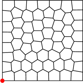
a

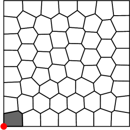
b

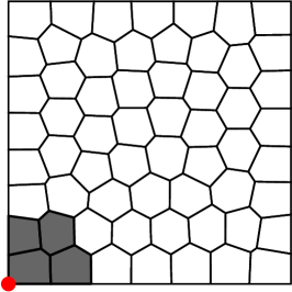
c

Fig. 1: Illustration of definition of $\mathcal{L}(z_{i},n)$: (a) Plot of $\mathcal{L}(z_{i},0)$; (b) Plot of $\mathcal{L}(z_{i},1)$; (c) Plot of $\mathcal{L}(z_{i},2)$.

It is easy to see that $\mathcal{L}(z_{i},n)$ consists of the mesh elements in the first n layers around the vertex $z_{i}$. In Figure 1, we give an illustration of $\mathcal{L}(z_{i},n)$ where $z_{i}$ is the red dotted point. From the figure, we can clearly observe that $\mathcal{L}(z_{i},0)$ just contains the vertex $z_{i}$ itself and $\mathcal{L}(z_{i},1)$ consists of the elements which have $z_{i}$ as a vertex; while $\mathcal{L}(z_{i},2)$ is the union of all elements in $\mathcal{L}(z_{i},1)$ and their neighbourhood elements.

Let $\Omega_{z_{i}}=\mathcal{L}(z_{i},n_{i})$ with $n_{i}$ be the smallest integer such that $\mathcal{L}(z_{i},n_{i})$ satisfies the rank condition in the following sense:

Definition 1.

A local patch $\Omega_{z_{i}}$ is said to satisfy the rank condition if it admits a unique least-squares fitted polynomial $p_{z_{i}}$ in (4.2).

Remark 2.

For virtual element methods, we are more interested in the case that $\mathcal{T}_{h}$ consists of polygons with more than four vertices. In general, to guarantee the rank condition we need $n_{i}=1$ for interior vertices and $n_{i}=2$ for boundary vertices.

Remark 3.

For boundary vertices, there are alternative ways to construct the local patch satisfying the rank condition in Definition 1. The readers are referred to [30].

To construct the recovered gradient at a given vertex $z_{i}$, let $B_{z_{i}}$ be the set of vertices in $\Omega_{z_{i}}$ and $I_{i}$ be the indexes of the $B_{z_{i}}$. Using the vertices in $B_{z_{i}}$ as sampling points, we fit a quadratic polynomial $p_{z_{i}}$ at the vertex $z_{i}$ in the following least-squares sense:

$$p_{z_{i}}(z)=\arg\min_{p\in\mathbb{P}_{2}(\Omega_{z_{i}})}\sum_{j\in I_{i}}|{p(z_{i_{j}})-u_{h,j}}|^{2},$$ (4.2)

where $u_{h,j}=u_{h}(z_{i_{j}})$.

To avoid numerical instability in real numerical computation, let

$$h_{i}=\max\{|z_{i_{k}}-z_{i_{j}}|:i_{k},i_{j}\in I_{i}\},$$

and define the local coordinate transform

$$F:(x,y)\rightarrow(\xi,\eta)=\frac{(x,y)-(x_{i},y_{i})}{h_{i}},$$ (4.3)

where $z=(x,y)$ and $\hat{z}=(\xi,\eta)$. All the computations are performed at the reference local element patch $\hat{\Omega}_{z_{i}}=F(\Omega_{z_{i}})$. Then we can rewrite $p_{z_{i}}(z)$ as

$$p_{z_{i}}(z)=\bm{p}^{T}\bm{a}=\hat{\bm{p}}^{T}\hat{\bm{a}},$$ (4.4)

where

$$\bm{p}^{T}=(1,x,y,x^{2},xy,y^{2}),\quad\hat{\bm{p}}^{T}=(1,\xi,\eta,\xi^{2},\xi\eta,\eta^{2}),$$

$$\bm{a}=(a_{1},a_{2},a_{3},a_{4},a_{5},a_{6}),\quad\hat{\bm{a}}=(a_{1},h_{i}a_{2},h_{i}a_{3},h_{i}^{2}a_{4},h_{i}^{2}a_{5},h_{i}^{2}a_{6}).$$

Let $\hat{z}_{i_{j}}=F(z_{i_{j}})$. The coefficient $\hat{\bm{a}}$ is determined by solving the linear system

$$(\hat{A}^{T}\hat{A})\hat{\bm{a}}=\hat{A}^{T}\bm{b},$$ (4.5)

where

$$\hat{A}=\left(\begin{matrix}1&\xi_{i_{1}}&\eta_{i_{1}}&\xi_{i_{1}}^{2}&\xi_{i_{1}}\eta_{i_{1}}&\eta_{i_{1}}^{2}\\ 1&\xi_{i_{2}}&\eta_{i_{2}}&\xi_{i_{2}}^{2}&\xi_{i_{2}}\eta_{i_{2}}&\eta_{i_{2}}^{2}\\ \vdots&\vdots&\vdots&\vdots&\vdots&\vdots\\ 1&\xi_{|I_{i}|}&\eta_{|I_{i}|}&\xi_{|I_{i}|}^{2}&\xi_{|I_{i}|}\eta_{|I_{i}|}&\eta_{|I_{i}|}^{2}\\ \end{matrix}\right)\text{ and }\bm{b}^{T}=\left(\begin{matrix}(u_{h})_{i_{1}}\\ (u_{h})_{i_{2}}\\ \cdots\\ (u_{h})_{i_{|I_{i}|}}\end{matrix}\right)$$

with $|I_{i}|$ being the cardinality of the set $I_{i}$.

Remark 4.

As observed in [24], the least-squares fitting procedure will not improve the accuracy of the solution approximation. We can remove one degree of freedom in the least-squares fitting procedure by assuming

$$\tilde{p}_{z_{i}}(z)\ =\ u_{h,i}+\tilde{a}_{2}(x-x_{i})+\tilde{a}_{3}(y-y_{i})+\tilde{a}_{4}(x-x_{i})^{2}+$$

$$\tilde{a}_{5}(x-x_{i})(y-y_{i})+\tilde{a}_{6}(y-y_{i})^{2}.$$

To determine $\tilde{\bm{a}}=(\tilde{a}_{2},\tilde{a}_{3},\cdots,\tilde{a}_{6})^{T}$, we only need to solve a $5\times 5$ linear system instead of $6\times 6$ linear system.

Then the recovered gradient $G_{h}u_{h}$ at the vertex $z_{i}$ is defined as

$$G_{h}u_{h}(z_{i})=\nabla p_{i}(z_{i})=\frac{1}{h_{i}}\left(\begin{matrix}\hat{a}_{2}\\ \hat{a}_{3}\end{matrix}\right).$$ (4.6)

Once we obtain $G_{h}u_{h}(z_{i})$ for each $i\in I_{h}$, the global recovered gradient can be interpolated as

$$G_{h}u_{h}=\sum_{i\in I_{h}}G_{h}u_{h}(z_{i})\phi_{i}.$$ (4.7)

Algorithm 1 Superconvergent Gradient Recovery Procedure

Let polygonal mesh $\mathcal{T}_{h}$ and the data (VEM solution) $(u_{h,i})_{i\in I_{h}}$ be given. Then repeat steps $(1)-(3)$ for all $i\in I_{h}$.

• For every $z_{i}$, construct a local patch of elements $\Omega_{z_{i}}$. Let $B_{z_{i}}$ be the set of vertices in $\Omega_{z_{i}}$ and $I_{i}$ be the indexes of the $B_{z_{i}}$.

• Construct reference local patch $\hat{\Omega}_{z_{i}}$ and reference set of vertices $\hat{B}_{z_{i}}$.

• Find a polynomial $\hat{p}_{z_{i}}$ over $\hat{\Omega}_{z_{i}}$ by solving the least squares problem

  $$\hat{p}_{z_{i}}=\arg\min_{\hat{p}}\sum_{j\in I_{i}}|{\hat{p}(\hat{z}_{i_{j}})-u_{h,j}}|^{2}\;\text{ for }\hat{p}\in\mathbb{P}_{2}(\hat{\Omega}_{z_{i}}).$$

• Calculate the partial derivatives of the approximated polynomial functions, then we have the recovered gradient at each vertex $z_{i}$

  $$G_{h}u_{h}(z_{i})=\nabla p_{z_{i}}(z_{i})=\frac{1}{h_{i}}\nabla\hat{p}_{z_{i}}(0,0).$$

For the recovery of the gradient $G_{h}u_{h}$ on the whole domain $\Omega$, we propose to interpolate the values ${G_{h}u_{h}(z_{i})}_{i\in I_{h}}$ by using the standard linear interpolation of the virtual element method.

The recovery procedure is summarized in Algorithm 1. From Algorithm 1, it can be clearly observed that to perform the gradient recovery procedure, we actually only use the information of degrees of freedom which is the only information directly available from the linear virtual element method.

For the purpose of theoretical analysis, we can also treat $G_{h}$ as an operator from $V_{h}$ to $V_{h}\times V_{h}$. It is easy to see that $G_{h}$ is a linear operator.

To show the consistency of the gradient recovery operator, we begin with the following theorem:

Theorem 5.

If $u$ is a quadratic polynomial on $\Omega_{z_{i}}$, then $G_{h}u(z_{i})=\nabla u(z_{i})$ for each $i\in I_{h}$.

Proof.

By the definition of (4.6), we only need to show

$$\nabla p_{z_{i}}(z_{i})=\nabla u(z_{i})$$ (4.8)

for all $u\in\mathbb{P}_{2}(\Omega_{z_{i}})$. To ease the presentation, we consider the least-squares fitting on the domain $\Omega_{z_{i}}$ instead of the local reference domain $\hat{\Omega}_{z_{i}}$. Suppose $\{q_{1}(z),q_{2}(z),\cdots,q_{6}(z)\}$ is the monomial basis of $\mathbb{P}_{2}(\Omega_{z_{i}})$ and let $\bm{p}=(q_{1}(z),q_{2}(z),\cdots,q_{6}(z))$. Then $p_{z_{i}}(z)=\bm{p}^{T}\bm{a}$ where $\bm{a}$ is determined by the linear system

$$A^{T}A\bm{a}=A^{T}\bm{b}.$$ (4.9)

To prove the polynomial preserving property, it is sufficient to show the equation (4.8) is true when $u=q_{j}(z)$ for $j=1,2,\cdots,6$. Let $u=q_{j}(z)$. Then it implies that

$$\bm{b}^{T}=\left(\begin{matrix}(q_{j})(z_{i_{1}})&(q_{j})(z_{i_{2}})&\cdots&(q_{j})(z_{i_{|I_{i}|}})\end{matrix}\right).$$ (4.10)

It is easy to see that $A\bm{e}_{j}=\bm{b}$ where $\bm{e}_{j}$ is the $j$th canonical basis function in $\mathbb{R}^{6}$. Note that $A^{T}A$ is nonsingular. Then $\bm{e}_{j}$ is the unique solution to the linear system (4.5). From (4.4), we can see that $p_{z_{i}}(z)=\bm{p}(z)^{T}\bm{e}_{j}=q_{j}(z)$ and hence $\nabla p_{z_{i}}(z_{i})=\nabla u(z_{i})$. Thus, for the quadratic polynomial $u$, we have $G_{h}u(z_{i})=\nabla u(z_{i})$. ∎

Theorem 5 means $G_{h}$ preserves quadratic polynomials at $z_{i}$. Using the polynomial preserving property above, we can show the following Lemma:

Lemma 6.

Suppose $u_{h}\in V_{h}$, then we have

$$|G_{h}u_{h}(z_{i})|\lesssim h^{-1}|u_{h}|_{1,\Omega_{z_{i}}}.$$ (4.11)

Proof.

According to (4.5) and (4.6), the recovered gradient $G_{h}u_{h}(z_{j})$ can be expressed as

$$G_{h}u_{h}(z_{i})=\left(\begin{matrix}G_{h}^{x}u_{h}(z_{i})\\ G_{h}^{y}u_{h}(z_{i})\end{matrix}\right)=\frac{1}{h_{i}}\left(\begin{matrix}\sum\limits_{j=1}^{|I_{i}|}\hat{c}_{j}^{1}u_{h,i_{j}}\\ \sum\limits_{j=1}^{|I_{i}|}\hat{c}_{j}^{2}u_{h,i_{j}}\end{matrix}\right),$$ (4.12)

where $\hat{c}_{j}^{k}$ is independent of the mesh size. Setting $u\equiv u_{h,i}$ in Theorem 5 yields

$$G_{h}u_{h}(z_{i})=\left(\begin{matrix}0\\ 0\end{matrix}\right).$$ (4.13)

Combining the above two equations, we have

$$G_{h}u_{h,i}=\frac{1}{h_{i}}\left(\begin{matrix}\sum\limits_{j=1}^{|I_{i}|}\hat{c}_{j}^{1}(u_{h,i_{j}}-u_{h,i})\\ \sum\limits_{j=1}^{|I_{i}|}\hat{c}_{j}^{2}(u_{h,i_{j}}-u_{h,i})\end{matrix}\right).$$ (4.14)

For any $z_{i_{j}}$, we can find $z_{i}=z_{j_{1}},z_{j_{2}},\cdots,z_{j_{n_{j}}}=z_{i_{j}}$ such that the line segment $\overline{z_{j_{\ell}}z_{j_{\ell+1}}}=e_{j_{\ell}}$ is an edge of an element $E\in\Omega_{z_{i}}$. Then we can rewrite $G^{x}_{h}u_{h}(z_{i})$ as

$$G^{x}_{h}u_{h}(z_{i})=\sum\limits_{j=1}^{|I_{i}|}\hat{c}_{j}^{1}\sum_{\ell=1}^{n_{j}-1}\frac{(u_{h,j_{\ell+1}}-u_{h,j_{\ell}})}{h_{i}}.$$ (4.15)

Note that $u_{h}$ is virtual element function. Then we have $u_{h}|_{e_{j_{\ell}}}$ is a linear polynomial and hence it holds that

$$\frac{u_{h,j_{\ell+1}}-u_{h,j_{\ell}}}{|e_{j_{\ell}}|}=\frac{\partial u_{h}}{\partial t_{j_{\ell}}}\leq|\nabla u_{h}|_{0,\infty,e_{j_{\ell}}},$$ (4.16)

where $t_{j_{\ell}}$ is the unit vector in the direction from $z_{j_{\ell}}$ to $z_{j_{\ell+1}}$. Substituting (4.16) into (4.15) gives

$$|G^{x}_{h}u_{h}(z_{i})|=\sum_{E\in\Omega_{z_{i}}}\sum_{e\in\mathcal{E}_{E}}\frac{|e|}{h_{i}}|\nabla u_{h}|_{0,\infty,e}.$$ (4.17)

Since $u_{h}|_{e}$ is a linear polynomial, the inverse inequality [15, 21] is applicable, which implies

$$|\nabla u_{h}|_{0,\infty,e}\lesssim|e|^{-\frac{3}{2}}||u_{h}||_{0,e}.$$ (4.18)

By the scaled trace inequality [14], we have

$$||u_{h}||_{0,e}\lesssim h^{-\frac{1}{2}}||u_{h}||_{0,E}+h^{\frac{1}{2}}|u_{h}|_{1,E}.$$ (4.19)

Combining the above estimates and noticing that $\frac{|e|}{h_{i}}$ is bounded by a fixed constant using the assumption (ii) on the mesh $\mathcal{T}_{h}$, we have

$$|G^{x}_{h}u_{h}(z_{i})|\lesssim \sum_{E\in\Omega_{z_{i}}}\left(h^{-2}||u_{h}||_{0,E}+h^{-1}|u_{h}|_{1,E}\right)$$

$$\lesssim h^{-2}||u_{h}||_{0,\Omega_{z_{i}}}+h^{-1}|u_{h}|_{1,\Omega_{z_{i}}}.$$

Let $\bar{u}_{h}=\frac{1}{|\Omega_{z_{i}}|}\int_{\Omega_{z_{i}}}u_{h}dz$. Setting $u_{h}\equiv\bar{u}_{h}$ in Theorem 5 implies $G_{h}\bar{u}_{h}(z_{i})=(0,0)^{T}$. Replacing $u_{h}$ by $u_{h}-\bar{u}_{h}$ in the above estimate, we have

$$|G^{x}_{h}u_{h}(z_{i})= |G^{x}_{h}(u_{h}-\bar{u}_{h})(z_{i})|$$

$$\lesssim h^{-2}||u_{h}-\bar{u}_{h}||_{0,\Omega_{z_{i}}}+h^{-1}|u_{h}-\bar{u}_{h}|_{1,\Omega_{z_{i}}}$$

$$\lesssim h^{-1}|u_{h}|_{1,\Omega_{z_{i}}},$$

where we have used the scaled Poincaré-Freidrichs inequality in [14].

Similarly, we can establish the same error bound for $G_{h}^{y}u_{h}(z_{i})$. Thus, the estimate (4.11) is true. ∎

Based on the above lemma, we can establish the local boundedness in $L_{2}$ norm:

Theorem 7.

Suppose $u_{h}\in V_{h}$, then for any $E\in\mathcal{T}_{h}$, we have

$$||G_{h}u_{h}||_{0,E}\lesssim|u_{h}|_{1,\Omega_{E}},$$ (4.20)

where $\Omega_{E}=\bigcup\limits_{z\in E\cap\mathcal{N}_{h}}\Omega_{z}$.

Proof.

Let $I_{E}$ be the index set of $E\cap\mathcal{N}_{h}$. Since $\{\phi_{i}\}_{i\in I_{h}}$ is the canonical basis for $V_{h}$, we have

$$\begin{split}||G_{h}u_{h}||_{0,E}\lesssim&|E|^{\frac{1}{2}}\sum_{j=1}^{|I_{E}|}|G_{h}u_{h}(z_{i_{j}})|\\ \lesssim&\sum_{j=1}^{|I_{E}|}|E|^{\frac{1}{2}}h^{-1}|u_{h}|_{1,\Omega_{z_{i_{j}}}}\\ \lesssim&|u_{h}|_{1,\Omega_{E}},\end{split}$$

where we have used the fact that $|E|^{\frac{1}{2}}h^{-1}$ is bounded by a fixed constant. ∎

As a direct consequence, we can prove the following corollary.

Corollary 8.

Suppose $u_{h}\in V_{h}$, then we have

$$||G_{h}u_{h}||_{0,\Omega}\lesssim|u_{h}|_{1,\Omega}.$$ (4.21)

Corollary 8 implies that $G_{h}$ is a linear bounded operator from $V_{h}$ to $V_{h}\times V_{h}$. Now, we are in the perfect position to present the consistency result of $G_{h}$.

Theorem 9.

Suppose $u\in H^{3}(\Omega_{E})$, then we have

$$\|G_{h}u-\nabla u\|_{0,E}\lesssim h^{2}\|u\|_{3,\Omega_{E}}.$$

Proof.

Define

$$\mathcal{F}(u)=\|G_{h}u-\nabla u\|_{0,E}.$$

By the boundedness of $G_{h}$, it is easy to see that

$$\begin{split}\mathcal{F}(u)\leq&\|G_{h}u\|_{0,E}+\|\nabla u\|_{0,E}\\ \lesssim&|u|_{1,\Omega_{E}}.\end{split}$$

The polynomial property of the gradient recovery operator $G_{h}$ implies $G_{h}p=\nabla p$ for any $p\in\mathbb{P}_{2}(\Omega_{E})$. Thus we have

$$\mathcal{F}(u+p)=\mathcal{F}(u).$$

By the Brambler-Hilbert Lemma[15, 21], we obtain

$$\mathcal{F}(u)\lesssim h^{2}\|u\|_{3,\Omega_{E}}.$$

∎

Theorem 9 implies the gradient recovery operator is consistent in the sense that the recovered gradient using the exact solution is superconvergent to the exact gradient at a rate of $\mathcal{O}(h^{2})$.

5 Adaptive Virtual Element Method

The adaptive virtual element method is summarized as a loop of the following steps:

$$\bf Solve\rightarrow Estimate\rightarrow Mark\rightarrow Refine$$ (5.1)

Starting from an initial polygonal mesh, we solve the equation by using the linear virtual element method. Once the virtual element solution is available, we need to design a fully computational a posteriori error estimator using only the virtual element solution. This step is vital for the adaptive virtual element method because it determines the performance of the adaptive algorithm. In this paper, we introduce a recovery-based a posteriori error estimator using the proposed gradient recovery method, which we elaborate in the coming subsection.

5.1 Recovery-based a posteriori error estimator

Provided that the recovered gradient is reconstructed, we are ready to present the recovery-type a posteriori error estimator for virtual element methods. However, for virtual element methods, their basis functions are not explicitly constructed which means that both $G_{h}u_{h}$ and $\nabla u_{h}$ are not computable quantities. To overcome this difficulty, we propose to use $\Pi^{0}_{E}G_{h}u_{h}$ and $\nabla\Pi^{0}_{E}u_{h}$, which are computable. We define a local a posteriori error estimator on each polygonal element E as

$$\eta_{h,E}=\|\Pi^{0}_{E}G_{h}u_{h}-\nabla\Pi^{0}_{E}u_{h}\|_{0,E},$$ (5.2)

and the corresponding global error estimator as

$$\eta_{h}=\left(\sum\limits_{E\in\mathcal{T}_{h}}\eta_{h,E}^{2}\right)^{1/2}.$$ (5.3)

To measure the performance of the a posteriori error estimator (5.2) or (5.3), we introduce the effective index

$$\kappa_{h}=\frac{\|\Pi^{0}_{E}G_{h}u_{h}-\nabla\Pi^{0}_{E}u_{h}\|_{0,\Omega}}{\|\nabla u-\nabla\Pi^{0}u_{h}\|_{0,\Omega}},$$ (5.4)

which is computable when the exact solution $u$ is provided.

For a posteriori error estimators, the ideal case we expect is the so-called asymptotic exactness.

Definition 10.

The a posteriori error estimator (5.2) or (5.3) is said to be asymptotically exact if

$$\lim_{h\rightarrow 0}\kappa_{h}=1.$$ (5.5)

A series of benchmark numerical examples in the next section indicate the recovery-based a posteriori error estimator (5.2) or (5.3) is asymptotically exact for the linear virtual element method, which distinguishes it from the residual-type a posteriori error estimators for virtual element methods in the literature [18, 12, 13].

5.2 Marking strategy

Once the recovery-type a posteriori error estimator $\eqref{equ:localind}$ is available, we pick up a set of elements to be refined. This process is called marking. There are several different marking strategies. In this paper, we adopt the bulk marking strategy proposed by Dörfler [25]. Given a constant $\theta\in(0,1]$, the bulk strategy is to find $\mathcal{M}_{h}\subset\mathcal{T}_{h}$ such that

$$\left(\sum_{E\in\mathcal{M}_{h}}\eta_{h,E}^{2}\right)^{\frac{1}{2}}\leq\theta\left(\sum_{E\in\mathcal{T}_{h}}\eta_{h,E}^{2}\right)^{\frac{1}{2}}.$$ (5.6)

In general, the choice of $\mathcal{M}_{h}$ is not unique. We select $\mathcal{M}_{h}$ such that the cardinality of $\mathcal{M}_{h}$ is smallest.

5.3 Adaptive mesh refinement

One of the main advantages of virtual element methods is their flexibility in local mesh refinement. Virtual element methods allow that elements can have an arbitrary number of edges and two edges can be collinear. These advantages enable virtual element methods to naturally handle hanging nodes. A polygon with a hanging node is just a polygon that has an extra edge collinear with another edge. It avoids artificial refinement of the unmarked neighborhood in the classical adaptive finite element methods. Take the polygon in Figure 2 as example. It is a pentagon with five vertices $V_{1},V_{2},\cdots,V_{5}$. But there are three hanging nodes $V_{6},V_{7},V_{8}$ which are generated by the refinement of its neighborhood element. In the virtual element method, we can treat the pentagon with three hanging nodes as an octagon with eight vertices $V_{1},V_{2},\cdots,V_{8}$. Note that in the octagon, there are four edges are collinear which is allowed in the virtual element method.

In the paper, we adopt the same way to refine a polygon as in [18, 49]. We divide a polygon into several sub-polygons by connecting its barycenter to each planar edge center. Note that two or more edges collinear to each other are treated as one planar edge. We take the polygon in Figure 2 as an example again. The refinement of the polygonal is illustrated in Figure 2 by the dashed lines. Note that the four edges collinear to each other are viewed as one edge $\overline{V_{5}V_{1}}$. Thus, in the refinement, we bisect $\overline{V_{5}V_{1}}$ instead of the four collinear edges.

Fig. 2: Illustration of handling hanging nodes in the virtual element method and local refinement of polygonals with collinear edges

6 Numerical Results

In this section, we present several numerical examples to demonstrate our numerical discoveries. The first example is to illustrate the superconvergence of the proposed gradient recovery. The other examples are to numerically validate the asymptotic exactness of the recovery-based a posteriori error estimator.

In the virtual element method, the basis functions are never explicitly constructed and the numerical solution is unknown inside elements. In the computational test, we shall use the projection $\Pi_{h}^{0}u_{h}$ to compute different errors instead of using $u_{h}$. In addition, all the convergence rates are illustrated in term of the degrees of freedom (DOF). In two dimensional cases, DOF $\approx h^{2}$ and the corresponding convergence rates in term of the mesh size $h$ are doubled of what we plot in the graphs.

6.1 Test case 1: smooth problem

In this example, we consider the following homogeneous elliptic equation

$$-\Delta u=2\pi^{2}\sin(\pi x)\sin(\pi y),\quad\text{ in }\Omega=(0,1)\times(0,1).$$ (6.1)

The exact solution is $u(x,y)=\sin(\pi x)\sin(\pi y)$.

a $\mathcal{T}_{h,1}$

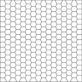
b $\mathcal{T}_{h,2}$

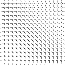
c $\mathcal{T}_{h,3}$

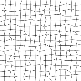
d $\mathcal{T}_{h,4}$

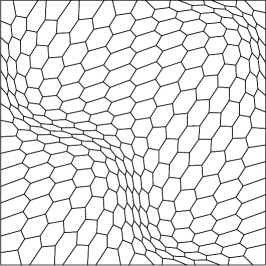
e $\mathcal{T}_{h,5}$

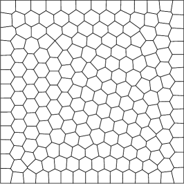
f $\mathcal{T}_{h,6}$

Fig. 3: Sample meshes for numerical tests: (a) uniform quadrilateral mesh; (b) structured hexagonal mesh; (c) concave mesh; (d) general quadrilateral mesh; (e) hexagonal mesh ; (f) Voronoi mesh.

In this test, we adopt six different types of meshes to numerically show the superconvergence of the proposed gradient recovery method. The first level of each type of meshes are plotted in Figure 3. The first type of mesh $\mathcal{T}_{h,1}$ is just the uniform square mesh. The second type of mesh $\mathcal{T}_{h,2}$ is uniform hexagonal mesh. The third type of mesh $\mathcal{T}_{h,3}$ is uniform non-convex mesh. $\mathcal{T}_{h,4}$ is generated by adding random perturbation to the mesh $\mathcal{T}_{h,1}$. The fifth type of mesh $\mathcal{T}_{h,5}$ is generated by applying the following coordinate transform

$$\begin{split}x=\hat{x}+\frac{1}{10}\sin(2\pi\hat{x})\sin(2\pi\hat{y}),\\ y=\hat{y}+\frac{1}{10}\sin(2\pi\hat{x})\sin(2\pi\hat{y});\\ \end{split}$$

to the uniform hexagonal mesh $\mathcal{T}_{h,2}$. The sixth type of mesh $\mathcal{T}_{h,6}$ is smoothed Voronoi mesh generated by Polymesher[48].

In addition to the discrete $H_{1}$ semi-error $\|\nabla u-\nabla\Pi^{0}_{h}u_{h}\|_{0,\Omega}$ and the recovered error $\|\nabla u-\Pi^{0}_{h}G_{h}u_{h}\|_{0,\Omega}$, we also consider the error $\|\nabla u_{h}-\nabla u_{I}\|_{0,\Omega}$. In this paper, we approximate $\|\nabla u_{h}-\nabla u_{I}\|_{0,\Omega}$ by a computable quantity $\sqrt{(\bm{u_{h}}-\bm{u_{I}})^{T}A_{h}(\bm{u_{h}}-\bm{u_{I}})}$ where $A_{h}$ is the stiffness matrix, $u_{I}$ is the interpolation of $u$ into the virtual element space $V_{h}$, and $\bm{u_{h}}$ (or $\bm{u_{I}}$) is a vector of value of $u_{h}$ (or $u_{I}$) on the degrees of freedom. The error $\|\nabla u_{h}-\nabla u_{I}\|_{0,\Omega}$ plays an important role in the study of superconvergence for gradient recovery methods in the classical finite element methods [6, 52]. We say the gradient of the numerical solution is superclose to the gradient of the interpolation of the exact solution if $\|\nabla u_{h}-\nabla u_{I}\|_{0,\Omega}\lesssim\mathcal{O}(h^{1+\rho})$ for some $0<\rho\leq 1$. The supercloseness result is a sufficient but not necessary condition to prove the superconvergence of gradient recovery methods [6, 52, 54, 27].

We plot the rates of convergence for the above three different errors in Figure 4. As predicted in [7], the discrete $H_{1}$ semi-error decays at a rate of $\mathcal{O}(h)$ for all the above six different types of meshes. Concerning the the error $\|\nabla u_{h}-\nabla u_{I}\|_{0,\Omega}$, we can only observe $\mathcal{O}(h^{2})$ supercloseness on two structured convex meshes and the transformed meshes $\mathcal{T}_{h,5}$. It is not surprising since the supercloseness depends strongly on the symmetry of meshes even on triangular meshes, see [6, 52]. But the recovered gradient is superconvergent to the exact gradient at a rate of $\mathcal{O}(h^{2})$ on all the above meshes including meshes with non-convex elements. The above numerical observation is summarized in Table 1.

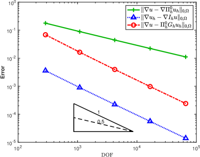
a $\mathcal{T}_{1}$

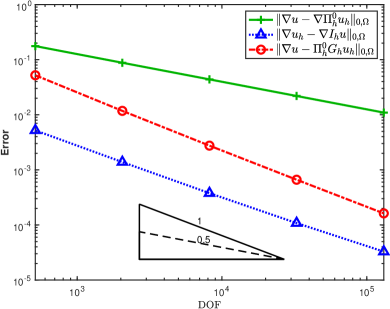
b $\mathcal{T}_{2}$

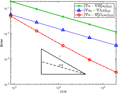
c $\mathcal{T}_{3}$

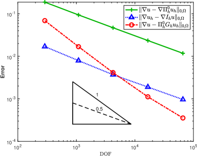
d $\mathcal{T}_{4}$

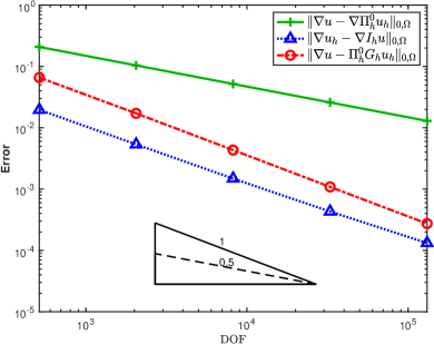
e $\mathcal{T}_{5}$

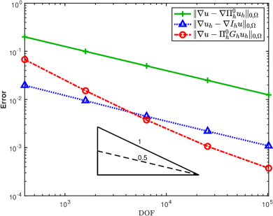
f $\mathcal{T}_{6}$

Fig. 4: Sample errors for numerical tests: (a) on structured quadrilateral mesh; (b) on structured hexagonal mesh; (c) on structure concave mesh; (d) on unstructured quadrilateral mesh; (e) on unstructured hexagonal mesh; (f) on unstructured Voronoi mesh.

Table 1: Summary of numerical results on the six different types of meshes

Mesh Type	$\|\nabla u-\Pi^{0}\nabla u_{h}\|_{0,\Omega}$	$\|\nabla u_{h}-\nabla u_{I}\|_{0,\Omega}$	$\|\nabla u-\Pi^{0}_{E}G_{h}u_{h}\|_{0,\Omega}$
$\mathcal{T}_{h,1}$	$\mathcal{O}(h)$	$\mathcal{O}(h^{2})$	$\mathcal{O}(h^{2})$
$\mathcal{T}_{h,2}$	$\mathcal{O}(h)$	$\mathcal{O}(h^{2})$	$\mathcal{O}(h^{2})$
$\mathcal{T}_{h,3}$	$\mathcal{O}(h)$	$\mathcal{O}(h)$	$\mathcal{O}(h^{2})$
$\mathcal{T}_{h,4}$	$\mathcal{O}(h)$	$\mathcal{O}(h)$	$\mathcal{O}(h^{2})$
$\mathcal{T}_{h,5}$	$\mathcal{O}(h)$	$\mathcal{O}(h^{2})$	$\mathcal{O}(h^{2})$
$\mathcal{T}_{h,6}$	$\mathcal{O}(h)$	$\mathcal{O}(h)$	$\mathcal{O}(h^{2})$

6.2 Test case 2: L-shaped domain problem

In this example, we consider the Laplace equation

$$-\Delta u=0,$$

on the L-shaped domain $\Omega=[-1,1]\times[-1,1]\backslash(0,1)\times(-1,0)$. The exact solution is $u=r^{2/3}\sin(2\theta/3)$ in polar coordinate. The corresponding boundary condition is computed from the exact solution $u$. Note the exact solution $u$ has a singularity at the origin.

a

b

Fig. 5: Meshes for test case 2: (a) Initial mesh; (b) Adaptively refined mesh.

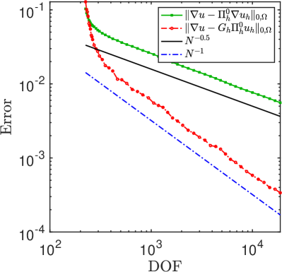
a

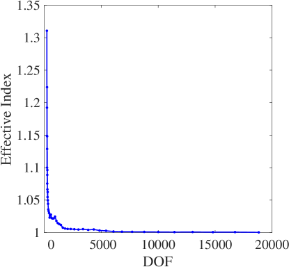
b

Fig. 6: Numerical result for test case 2: (a) Numerical errors; (b) Effective index.

To resolve the singularity, we use the adaptive virtual element method described in Section 5. The initial mesh is plotted in Figure 5a, which is a uniform mesh consisting of square elements. In Figure 5b, we show the corresponding adaptively refined mesh. It is not hard to see that the refinement is conducted near the singular point.

In Figure 6a, we depict the rates of convergence for discrete $H_{1}$ semi-error $\|\nabla u-\nabla\Pi^{0}_{h}u_{h}\|_{0,\Omega}$ and the discrete recovery error $\|\nabla u-\Pi^{0}_{h}G_{h}u_{h}\|_{0,\Omega}$. From the plot, we can clearly observe $\mathcal{O}(h)$ optimal convergence for the virtual element gradient and $\mathcal{O}(h^{2})$ superconvergence for the recovered gradient for the adaptive virtual element method. It means the recovery-based a posteriori error estimator (5.2) is robust. To quantify the performance of the error estimator, we draw the effective index (5.4) in Figure 6b. It shows that the effective index converges to 1 rapidly after a few iterations. It means the a posteriori error estimator is asymptotically exact as defined in Definition 10.

a

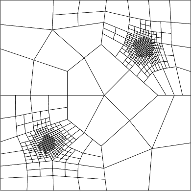
b

Fig. 7: Meshes for test case 3: (a) Initial mesh; (b) Adaptively refined mesh.

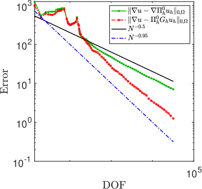
a

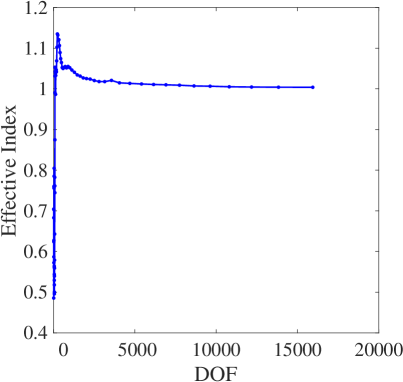
b

Fig. 8: Numerical result for test case 3: (a) Numerical errors; (b) Effective index.

6.3 Test case 3: problem with two Gaussian surfaces

Consider the Poisson equation (2.1) on the unit square with the exact solution

$$u(x,y)=\frac{1}{2\pi\sigma}\left[e^{-\frac{1}{2}\left(\frac{x-\mu_{1}}{\sigma}\right)^{2}}e^{-\frac{1}{2}\left(\frac{y-\mu_{1}}{\sigma}\right)^{2}}+e^{-\frac{1}{2}\left(\frac{x-\mu_{2}}{\sigma}\right)^{2}}e^{-\frac{1}{2}\left(\frac{y-\mu_{2}}{\sigma}\right)^{2}}\right]$$

as in [49]. In this test, the standard deviation is $\sigma=\sqrt{10^{-3}}$ and the two means are $\mu_{1}=0.25$ and $\mu_{2}=0.75$.

The difficulty of this problem is the existence of two Gaussian surfaces, where the solution has a fast decay. Here we adopt the same initial mesh as in [49], see Figure 7a. It is a polygonal mesh, which does not resolve the Gaussian surfaces. In Figure 7b, we show the adaptively refined mesh. Clearly, the mesh is refined near the location of the Gaussian surfaces. In Figure 8a, we present the numerical errors. Similar to test case 2, we can observe the desired optimal and superconvergent results. Moreover, the asymptotic exactness of the error estimator (5.2) is numerically verified in Figure 8b by the fact that the effective index is convergent to one.

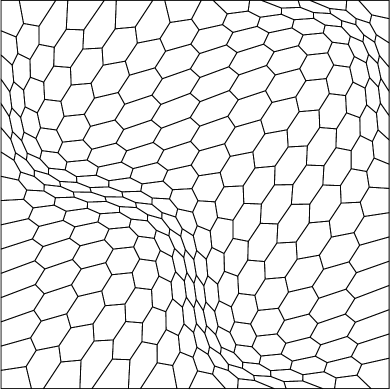
a

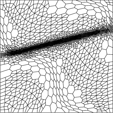
b

Fig. 9: Meshes for test case 4: (a) Initial mesh; (b) Adaptively refined mesh.

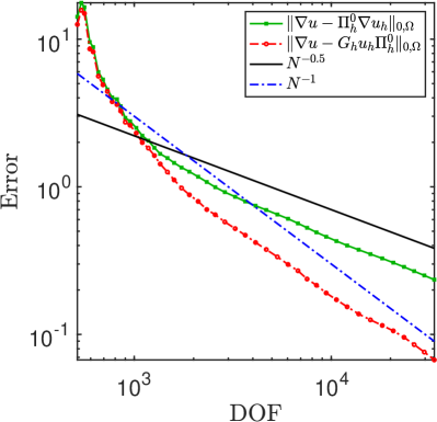
a

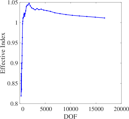
b

Fig. 10: Numerical result for test case 4: (a) Numerical errors; (b) Effective index.

6.4 Test case 4: problem with sharp interior layer

As in [18, 12], we consider the Poisson equation (2.1) and (2.2) on the unit square with a sharp interior layer. The exact solution is

$$u(x,y)=16x(1-x)y(1-y)\arctan(25x-100y+25).$$

The initial mesh is the transformed hexagonal mesh $\mathcal{T}_{h,5}$ as in Test Case 1, which is shown in Figure 9a. It is an unstructured polygonal mesh. The interior sharp layer is totally unresolved by the initial mesh which causes the major difficulty. Figure 9b is the mesh generated by the adaptive virtual element method prescribed in Section 5. It is obvious that the mesh is refined to resolve the interior layer as expected.

In Figure 10, we present the qualitative results. As anticipated, the desired $\mathcal{O}(h)$ optimal convergence rate for the virtual element gradient and $\mathcal{O}(h^{2})$ superconvergence rate for the recovered gradient can be numerically observed. Also, the limit of the effective index is numerically proved to be one, which validates the asymptotic exactness of the error estimator (5.2).

7 Conclusion

In this paper, a superconvergent gradient recovery method for the virtual element methods is introduced. The proposed post-processing technique uses only the degrees of freedom which are the only data directly obtained from the virtual element methods. It generalizes the idea of polynomial preserving recovery [54, 40] to general polygonal meshes. Theoretically, we prove the proposed gradient recovery method is bounded and consistent. It meets the standard of a good gradient recovery technique in [2]. Numerically, we validated the superconvergence of the recovered gradient using the virtual element solution on several different types of general polygonal meshes including meshes with non-convex elements. In the future, it would be interesting to present a theoretical proof of those superconvergence for the virtual element method.

Its capability of serving as a posteriori error estimators is also exploited. The asymptotic exactness of the recovery-based a posteriori error estimator is numerically verified by three benchmark problems. To the best of our knowledge, it is the first recovery-based a posteriori error estimator for the virtual element methods. Compared to the existing residual type a posteriori error estimators, it has several advantages: (i) it is simple in both the idea and implementation, which makes it more realistic for practical applications; (ii) the unique characterization of the error estimator is asymptotic exactness, which prevails over all other a posteriori error estimators in the literature for the virtual element methods.

The application of gradient recovery is not limited to adaptive methods. It has also been applied to many other fields, like enhancing eigenvalues[42, 41, 29] and designing new numerical methods for higher order PDEs[20, 31, 32, 53]. We will make use of those advantages of gradient recovery to study more interesting real application problems in future work.

Ackowledgement

The authors thank the anonymous referees for their comments and suggestions which significantly improve the quality of this paper.

References

- [1] B. Ahmad, A. Alsaedi, F. Brezzi, L. D. Marini, and A. Russo, Equivalent projectors for virtual element methods, Comput. Math. Appl., 66 (2013), pp. 376–391.
- [2] M. Ainsworth and J. T. Oden, A posteriori error estimation in finite element analysis, Pure and Applied Mathematics (New York), Wiley-Interscience [John Wiley & Sons], New York, 2000.
- [3] E. Artioli, S. de Miranda, C. Lovadina, and L. Patruno, A stress/displacement virtual element method for plane elasticity problems, Comput. Methods Appl. Mech. Engrg., 325 (2017), pp. 155–174.
- [4] I. Babuška and T. Strouboulis, The finite element method and its reliability, Numerical Mathematics and Scientific Computation, The Clarendon Press, Oxford University Press, New York, 2001.
- [5] I. Babuška and W. C. Rheinboldt, Error estimates for adaptive finite element computations, SIAM J. Numer. Anal., 15 (1978), pp. 736–754.
- [6] R. E. Bank and J. Xu, Asymptotically exact a posteriori error estimators. I. Grids with superconvergence, SIAM J. Numer. Anal., 41 (2003), pp. 2294–2312 (electronic).
- [7] L. Beirão da Veiga, F. Brezzi, A. Cangiani, G. Manzini, L. D. Marini, and A. Russo, Basic principles of virtual element methods, Math. Models Methods Appl. Sci., 23 (2013), pp. 199–214.
- [8] L. Beirão da Veiga, F. Brezzi, L. D. Marini, and A. Russo, The hitchhiker’s guide to the virtual element method, Math. Models Methods Appl. Sci., 24 (2014), pp. 1541–1573.
- [9] , Virtual element method for general second-order elliptic problems on polygonal meshes, Math. Models Methods Appl. Sci., 26 (2016), pp. 729–750.
- [10] L. Beirão da Veiga, K. Lipnikov, and G. Manzini, Arbitrary-order nodal mimetic discretizations of elliptic problems on polygonal meshes, SIAM J. Numer. Anal., 49 (2011), pp. 1737–1760.
- [11] L. Beirão da Veiga, K. Lipnikov, and G. Manzini, The mimetic finite difference method for elliptic problems, vol. 11 of MS&A. Modeling, Simulation and Applications, Springer, Cham, 2014.
- [12] L. Beirão da Veiga and G. Manzini, Residual a posteriori error estimation for the virtual element method for elliptic problems, ESAIM Math. Model. Numer. Anal., 49 (2015), pp. 577–599.
- [13] S. Berrone and A. Borio, A residual a posteriori error estimate for the Virtual Element Method, Math. Models Methods Appl. Sci., 27 (2017), pp. 1423–1458.
- [14] S. C. Brenner, Q. Guan, and L.-Y. Sung, Some estimates for virtual element methods, Comput. Methods Appl. Math., 17 (2017), pp. 553–574.
- [15] S. C. Brenner and L. R. Scott, The mathematical theory of finite element methods, vol. 15 of Texts in Applied Mathematics, Springer, New York, third ed., 2008.
- [16] F. Brezzi, A. Buffa, and K. Lipnikov, Mimetic finite differences for elliptic problems, ESAIM: Math. Model. Numer. Anal., 43 (2009), pp. 277–295.
- [17] F. Brezzi and L. D. Marini, Virtual element methods for plate bending problems, Comput. Methods Appl. Mech. Engrg., 253 (2013), pp. 455–462.
- [18] A. Cangiani, E. H. Georgoulis, T. Pryer, and O. J. Sutton, A posteriori error estimates for the virtual element method, Numer. Math., 137 (2017), pp. 857–893.
- [19] A. Cangiani, G. Manzini, and O. J. Sutton, Conforming and nonconforming virtual element methods for elliptic problems, IMA J. Numer. Anal., 37 (2017), pp. 1317–1354.
- [20] H. Chen, H. Guo, Z. Zhang, and Q. Zou, A linear finite element method for two fourth-order eigenvalue problems, IMA J. Numer. Anal., 37 (2017), pp. 2120–2138.
- [21] P. G. Ciarlet, The finite element method for elliptic problems, vol. 40 of Classics in Applied Mathematics, Society for Industrial and Applied Mathematics (SIAM), Philadelphia, PA, 2002. Reprint of the 1978 original [North-Holland, Amsterdam; MR0520174 (58 #25001)].
- [22] D. A. Di Pietro and A. Ern, A hybrid high-order locking-free method for linear elasticity on general meshes, Comput. Methods Appl. Mech. Engrg., 283 (2015), pp. 1–21.
- [23] D. A. Di Pietro, A. Ern, and S. Lemaire, An arbitrary-order and compact-stencil discretization of diffusion on general meshes based on local reconstruction operators, Comput. Methods Appl. Math., 14 (2014), pp. 461–472.
- [24] G. Dong and H. Guo, Parametric polynomial preserving recovery on manifolds, arXiv:1703.06509 [math.NA], 2017.
- [25] W. Dörfler, A convergent adaptive algorithm for Poisson’s equation, SIAM J. Numer. Anal., 33 (1996), pp. 1106–1124.
- [26] L. C. Evans, Partial differential equations, vol. 19 of Graduate Studies in Mathematics, American Mathematical Society, Providence, RI, second ed., 2010.
- [27] H. Guo and Z. Zhang, Gradient recovery for the Crouzeix-Raviart element, J. Sci. Comput., 64 (2015), pp. 456–476.
- [28] H. Guo, Z. Zhang, and R. Zhao, Hessian recovery for finite element methods, Math. Comp., 86 (2017), pp. 1671–1692.
- [29] , Superconvergent two-grid methods for elliptic eigenvalue problems, J. Sci. Comput., 70 (2017), pp. 125–148.
- [30] H. Guo, Z. Zhang, R. Zhao, and Q. Zou, Polynomial preserving recovery on boundary, J. Comput. Appl. Math., 307 (2016), pp. 119–133.
- [31] H. Guo, Z. Zhang, and Q. Zou, A linear finite element method for biharmonic problems, J. Sci. Comput., 74 (2018), pp. 1397–1422.
- [32] , A linear finite element method for sixth order elliptic equations, arXiv:1804.03793 [math.NA], 2018.
- [33] J. M. Hyman and M. Shashkov, Mimetic discretizations for Maxwell’s equations, J. Comput. Phys., 151 (1999), pp. 881–909.
- [34] Yu. Kuznetsov and S. Repin, New mixed finite element method on polygonal and polyhedral meshes, Russian J. Numer. Anal. Math. Modelling, 18 (2003), pp. 261–278.
- [35] A. M. Lakhany, I. Marek, and J. R. Whiteman, Superconvergence results on mildly structured triangulations, Comput. Methods Appl. Mech. Engrg., 189 (2000), pp. 1–75.
- [36] G. Manzini, A. Russo, and N. Sukumar, New perspectives on polygonal and polyhedral finite element methods, Math. Models Methods Appl. Sci., 24 (2014), pp. 1665–1699.
- [37] D. Mora, G. Rivera, and R. Rodrí guez, A posteriori error estimates for a virtual element method for the Steklov eigenvalue problem, Comput. Math. Appl., 74 (2017), pp. 2172–2190.
- [38] L. Mu, J. Wang, Y. Wang, and X. Ye, Interior penalty discontinuous Galerkin method on very general polygonal and polyhedral meshes, J. Comput. Appl. Math., 255 (2014), pp. 432–440.
- [39] A. Naga and Z. Zhang, A posteriori error estimates based on the polynomial preserving recovery, SIAM J. Numer. Anal., 42 (2004), pp. 1780–1800 (electronic).
- [40] , The polynomial-preserving recovery for higher order finite element methods in 2D and 3D, Discrete Contin. Dyn. Syst. Ser. B, 5 (2005), pp. 769–798.
- [41] , Function value recovery and its application in eigenvalue problems, SIAM J. Numer. Anal., 50 (2012), pp. 272–286.
- [42] A. Naga, Z. Zhang, and A. Zhou, Enhancing eigenvalue approximation by gradient recovery, SIAM J. Sci. Comput., 28 (2006), pp. 1289–1300.
- [43] S. Repin, A posteriori estimates for partial differential equations, vol. 4 of Radon Series on Computational and Applied Mathematics, Walter de Gruyter GmbH & Co. KG, Berlin, 2008.
- [44] M. Shashkov, Conservative finite-difference methods on general grids, Symbolic and Numeric Computation Series, CRC Press, Boca Raton, FL, 1996. With 1 IBM-PC floppy disk (3.5 inch; HD).
- [45] M. Shashkov and S. Steinberg, Solving diffusion equations with rough coefficients in rough grids, J. Comput. Phys., 129 (1996), pp. 383–405.
- [46] N. Sukumar and E. A. Malsch, Recent advances in the construction of polygonal finite element interpolants, Arch. Comput. Methods Engrg., 13 (2006), pp. 129–163.
- [47] N. Sukumar and A. Tabarraei, Conforming polygonal finite elements, Internat. J. Numer. Methods Engrg., 61 (2004), pp. 2045–2066.
- [48] C. Talischi, G. H. Paulino, A. Pereira, and I. F. M. Menezes, PolyMesher: a general-purpose mesh generator for polygonal elements written in Matlab, Struct. Multidiscip. Optim., 45 (2012), pp. 309–328.
- [49] A. Vaziri Astaneh, F. Fuentes, J. Mora, and L. Demkowicz, High-order polygonal discontinuous Petrov–Galerkin (PolyDPG) methods using ultraweak formulations, Comput. Methods Appl. Mech. Engrg., 332 (2018), pp. 686–711.
- [50] R. Verfürth, A posteriori error estimation techniques for finite element methods, Numerical Mathematics and Scientific Computation, Oxford University Press, Oxford, 2013.
- [51] E. L. Wachspress, A rational finite element basis, Academic Press, Inc. [A subsidiary of Harcourt Brace Jovanovich, Publishers], New York-London, 1975. Mathematics in Science and Engineering, Vol. 114.
- [52] J. Xu and Z. Zhang, Analysis of recovery type a posteriori error estimators for mildly structured grids, Math. Comp., 73 (2004), pp. 1139–1152 (electronic).
- [53] M. Xu, H. Guo, and Q. Zou, Hessian recovery based finite element methods for the Cahn-Hilliard equation, J. Comput. Phys., 386 (2019), pp. 524–540.
- [54] Z. Zhang and A. Naga, A new finite element gradient recovery method: superconvergence property, SIAM J. Sci. Comput., 26 (2005), pp. 1192–1213 (electronic).
- [55] O. C. Zienkiewicz and J. Z. Zhu, A simple error estimator and adaptive procedure for practical engineering analysis, Internat. J. Numer. Methods Engrg., 24 (1987), pp. 337–357.
- [56] , The superconvergent patch recovery and a posteriori error estimates. I. The recovery technique, Internat. J. Numer. Methods Engrg., 33 (1992), pp. 1331–1364.
- [57] , The superconvergent patch recovery and a posteriori error estimates. II. Error estimates and adaptivity, Internat. J. Numer. Methods Engrg., 33 (1992), pp. 1365–1382.