Detection of Reflection Features in the Neutron Star Low-Mass X-ray Binary Serpens X-1 with NICER

Abstract

We present Neutron Star Interior Composition Explorer (NICER) observations of the neutron star low-mass X-ray binary Serpens X-1 during the early mission phase in 2017. With the high spectral sensitivity and low-energy X-ray passband of NICER, we are able to detect the Fe L line complex in addition to the signature broad, asymmetric Fe K line. We confirm the presence of these lines by comparing the NICER data to archival observations with XMM-Newton/RGS and NuSTAR. Both features originate close to the innermost stable circular orbit (ISCO). When modeling the lines with the relativistic line model relline, we find the Fe L blend requires an inner disk radius of $1.4_{-0.1}^{+0.2}$ $R_{\mathrm{ISCO}}$ and Fe K is at $1.03_{-0.03}^{+0.13}$ $R_{\mathrm{ISCO}}$ (errors quoted at 90%). This corresponds to a position of $17.3_{-1.2}^{+2.5}$ km and $12.7_{-0.4}^{+1.6}$ km for a canonical neutron star mass ($M_{\mathrm{NS}}=1.4\ M_{\odot}$) and dimensionless spin value of $a=0$. Additionally, we employ a new version of the relxill model tailored for neutron stars and determine that these features arise from a dense disk and supersolar Fe abundance.

1. Introduction

In low-mass X-ray binary (LMXB) systems, where the companion star has mass $\leq 1\ \mathrm{M}_{\odot}$, accretion onto the compact object generally occurs through an accretion disk formed via Roche-lobe overflow. In many instances, these disks are illuminated by hard X-rays coming either from a hot electron corona (Sunyaev et al., 1991) or the surface of the neutron star or boundary layer (where the material from the disk reaches the neutron star; Popham & Sunyaev 2001). The exact location and geometry of the corona is not known, but is considered to be compact and close to the compact object (see Degenaar et al. 2018 for a review and references therein). Regardless of the source of the hard X-rays, the disk reprocesses the illuminating photons and re-emits them in a continuum with a series of atomic features and Compton backscattering hump superimposed, known as the “reflection” spectrum. The most prominent feature that arises as a result of reflection is the Fe K emission line between 6.4–6.97 keV. The entire Fe line profile is shaped by strong Doppler and relativistic effects due to the disk’s rotational velocity and proximity to the compact object (Fabian et al., 1989). The extent of the red wing thereby enables important physical insights to be derived from these systems. Moreover, the blue-shifted emission of the Fe line profile provides an indication of the inclination of the disk due to Doppler effects becoming more prominent with increasing inclination (Dauser et al., 2010). This feature has been reported in both black hole (BH: e.g., Miller 2002) and neutron star (NS: e.g., Bhattacharyya & Strohmayer 2007; Cackett et al. 2008) LMXBs, suggesting similar accretion geometries despite the mass difference of the compact accretor and the presence of a surface.

An additional prominent reflection feature that can arise from the illuminated accretion disk is the lower-energy Fe L line near $1$ keV. This feature was first reported in Fabian et al. (2009) for the active galactic nucleus (AGN) 1H0707$-$495 with the same asymmetric broadening seen in Fe K. Moreover, the ratio of Fe K to Fe L emission was consistent with predictions from atomic physics. This feature was soon discovered in other AGN, such as IRAS 13224$-$3809 (Ponti et al. 2010), cementing the importance of reflection features in these accreting systems.

The BHs in LMXBs are scaled-down versions of the much more massive accretors in AGN (Miller, 2007). Since accretion in BH and NS LMXBs is similar, we expect to find an Fe L feature in a NS LMXB if the conditions are right. There have been a number of reports of line complexes near $\sim 1$ keV in NS LMXBs during persistent emission that have been attributed to the Fe L transition, but also K-shell transitions of medium-Z elements (Vrtilek et al. 1988; Kuulkers et al. 1997; Schulz 1999; Sidoli et al. 2001; Cackett et al. 2010). These lines appear to be broadened by the same mechanism as the Fe K component (Ng et al., 2010) and can be modeled as smeared relativistic lines (Iaria et al., 2009).

Serpens X-1 (Ser X-1) is an “atoll” NS LMXB located at a distance of $7.7\pm 0.9$ kpc (Galloway et al., 2008). Optical spectroscopy and some X-ray reflection studies indicate that the system has a low binary inclination ($i\leq 10^{\circ}$, Cornelisse et al. 2013; Miller et al. 2013), though higher inclinations have been reported from other X-ray reflection studies ($25^{\circ}<i<50^{\circ}$, Cackett et al. 2008, 2010; Chiang et al. 2016; Matranga et al. 2017). The low amount of absorbing material in the direction of Ser X-1, as demonstrated by the low neutral hydrogen column density ($\mathrm{N}_{\mathrm{H}}=4\times 10^{21}$ cm^-2, Dickey & Lockman 1990), provides an opportunity to detect multiple reflection features.

With the recent launch of the Neutron Star Interior Composition Explorer (NICER; Gendreau et al. 2012), we now have the opportunity to test reflection predictions and probe the innermost region of the accretion disk in Ser X-1. NICER was installed on the International Space Station in 2017 June. The payload comprises 56 “concentrator” optics that each focus X-rays in the 0.2–12 keV range onto a paired silicon drift detector. Prelaunch testing left 52 functioning detectors providing a total collecting area of $1900$ cm² at 1.5 keV with which to search for low-energy reflection features.

2. Observations and Data Reduction

The following subsections detail the reduction of Ser X-1 observations obtained with NICER, NuSTAR, and XMM-Newton. The NuSTAR and XMM-Newton data were not acquired contemporaneously with our NICER observations, but are used as a baseline for determining which features are astrophysical in the NICER data, since Ser X-1 has remained roughly steady in its persistent emission (0.2–0.3 Crab) in the Swift/BAT and MAXI wide-field monitors for the past decade.

2.1. NICER

NICER observed Ser X-1 thirteen times between 2017 July and 2017 November (ObsIDs 1050320101–1050320113) for a cumulative exposure of 39.9 ks on target. The data were reduced using NICERDAS version 2018-02-22_V002d. Good time intervals (GTIs) were created using nimaketime selecting COR_SAX$\geq$4, to remove high particle radiation intervals associated with the Earth’s auroral zones, and separating orbit day (SUNSHINE==1) from orbit night (SUNSHINE==0) in addition to the standard NICER filtering criteria. Moreover, we only selected events that occurred when the angle between the Sun and target of observation were $\geq 90^{\circ}$. These GTIs were applied to the data via niextract-events selecting events with PI channel between 25 and 1200 (0.25–12.0 keV) that triggered the detector readout system’s slow and, optionally, fast signal chains. Background spectra were created from data acquired from one of seven “blank sky” targets based on RXTE background fields (Jahoda et al., 2006). We reduced all observations of the background fields as described above. Ser X-1 is much brighter (1597 counts s^-1) in comparison to the background fields ( $\sim 0.7-2.3$ counts s^-1). We proceeded with using RXTE background field 5 throughout the remaining analysis since the results are not dependent upon this choice.

The resulting event files were read into xselect and combined to create light-curves and time-averaged spectra for orbit day and orbit night. There were no Type-I X-ray bursts present in the light-curves during the GTIs so no additional filtering was needed. The spectra suffered from instrumental residuals given the preliminary calibration at this stage. In order to mitigate these residuals we normalized the data to NICER observations of the Crab Nebula, which has a featureless absorbed power-law spectrum in the energy range of interest (see, e.g., Weisskopf et al. 2010).

We use ObsIDs 1011010101, 1011010201, and 1013010101-1013010123 for the Crab, and the same data reduction procedure as above. The resulting exposure time for the Crab is $\sim 1.1$ ks for orbit day and $\sim 21.2$ ks for orbit night. The time-averaged Crab spectrum was fit with an absorbed power-law model from 0.25–10 keV to determine the absorption column along the line of sight. The absorption column was consistent with the Dickey & Lockman (1990) value at $\mathrm{N}_{\mathrm{H}}\sim 3.8\times 10^{21}$ cm^-2. We then froze the absorption column and fit the 3–10 keV subset of the spectrum to prevent instrumental features at low energies from skewing the fit. This returned a photon index of $\Gamma\sim 2.0$. We extrapolated the fit back down to 0.25 keV and created a fake spectrum using the ‘fakeit’ command within the xspec software package (Arnaud, 1996) for the same exposure time as the actual Crab data. We used the ftool mathpha to divide the Crab spectrum by the simulated Crab data. This yielded a spectrum with just the instrumental residuals. We then used mathpha to divide the Ser X-1 count rate spectrum by the instrumental residual spectrum. The normalized spectra after applying all of our filtering criteria for orbit night and day have exposures of $\sim 4.5$ ks and $\sim 4.7$ ks, respectively. However, since the exposure time for the Crab during orbit day was much smaller in comparison to orbit night, it introduced noise into the Ser X-1 spectrum when normalizing. We therefore only focused on the data that was accumulated during orbit night. See Figure 1 for a comparison of the Ser X-1 data before and after normalizing to the Crab. The source spectrum was grouped via grppha to have a minimum of 25 counts per bin.

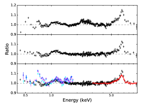
Figure 1.— Top: Ratio of NICER data to continuum before normalizing to the Crab. Instrumental residuals can be seen at $\sim 0.5$ keV, $\sim 1.8$ keV, and $\sim 2.2$ keV due to O, Si, and Au, respectively. The feature at $\sim 0.7$ keV has instrumental origin as well, likely due to gain offsets as the response changes rapidly in this area. Middle: Ratio of NICER data to continuum after normalizing to the Crab to mitigate instrumental residuals. Emission features are still present near $1.1$ keV and $6.7$ keV. Bottom: Ratio of the data to continuum model for NICER (black), NuSTAR (red), and XMM-Newton/RGS (blue, cyan, purple) observations. The data were fit with the combination of an absorbed single-temperature blackbody, multi-temperature blackbody, and power-law. The $0.9-1.3$ keV and $5.0-8.0$ keV energy bands were ignored while fitting to prevent the lines from skewing the continuum. Continuum parameters were tied between NICER and NuSTAR while normalization components were allowed to vary. The XMM-Newton data were left free with a constant allowed to float between observations. Data were rebinned for clarity.

2.2. NuSTAR

Two observations of Ser X-1 were taken with NuSTAR on 2013 July 12 and 13 (ObsIDs 30001013002 and 30001013004) for $\sim 30.5$ ks. These observations have been previously reported by Miller et al. (2013) and Matranga et al. (2017). There were no Type-I X-ray bursts that occurred during the 2013 observations. Using the nuproducts tool from nustardas v1.8.0 with caldb 20180126, we created light-curves and spectra for the 2013 observations with statusexpr=“STATUS==b0000xxx00xxxx000” to correct for high count rates. We used a circular extraction region with a radius of 100^′′ centered around the source to produce a source spectrum for both the FPMA and FPMB. We used another 100^′′ radial region away from the source for the purpose of background subtraction. Following Miller et al. (2013), we respectively combined the two source spectra, background spectra, ancillary response matrices and redistribution matrix files via addascaspec and addrmf, weighting by exposure time. The combined spectra were grouped to have a minimum of 100 counts per bin using grppha.

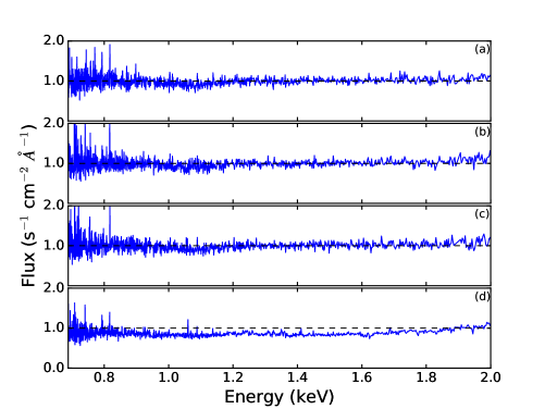
Figure 2.— Ratio of RGS first to second order fluxed spectra for the three XMM-Newton observations: (a) 0084020401, (b) 0084020501, and (c) 0084020601. The bottom panel denoted (d) shows an observation of GRO J1655-40 that is piled-up. The ratio is roughly consistent with unity in panels (a)-(c) indicating that pile-up in the RGS band is not an issue for Serpens X-1.

2.3. XMM-Newton

There are three observations of Ser X-1 with XMM-Newton (ObsIDs 0084020401, 0084020501, and 0084020601) performed in 2004 March for a total exposure of $\sim 65.7\ \mathrm{ks}$. These observations were reported in Bhattacharyya & Strohmayer (2007), Cackett et al. (2010), and Matranga et al. (2017). We focus on the Reflection Grating Spectrometer (RGS) data because we are interested in the high-resolution, low-energy spectral features. The data were reduced using the command rgsproc in SAS v16.1. We checked that the data do not suffer from pile-up by inspecting the ratio of the first and second order fluxed spectra (see Figure 2). Each ratio for Ser X-1 is consistent with unity across nearly all of the RGS energy band indicating that pile-up is not an issue. For comparison, we plot the ratio of the fluxed spectra for the stellar mass black hole X-ray binary GRO J1655-40, which suffered from pile-up in the RGS instrument, in the bottom panel. Since the observations of Ser X-1 were not piled-up, the first order RGS1 and RGS2 data were combined via rgscombine for each respective observation. The resulting spectra were then grouped using grppha to have a minimum of 25 counts per bin.

3. Spectral Analysis and Results

We use xspec version 12.9.1m and report uncertainties at the 90% confidence level. Since the XMM-Newton and NuSTAR data have been previously analyzed and published elsewhere, we choose to mainly focus on the NICER results. We model the NICER data in the $0.4-10.0$ keV energy band, outside of which the effective area drops sharply. We model the absorption along the line of sight using tbnew with vern cross sections (Verner et al., 1996) and wilm abundances (Wilms et al., 2000). We allow the neutral hydrogen absorption, as well as the oxygen and iron absorption abundances, to be free parameters to ensure that edges in the region of interest are properly modeled. Allowing the oxygen and iron absorption to deviate from solar abundance provides a statistical improvement in the following fits at more than $9\sigma$ confidence level in each case, although these could be instrumental in origin as the O K edge lines up with changes in the effective area of the detector and may not reflect actual ISM abundance measurements. We find a neutral absorption column of $\mathrm{N}_{\mathrm{H}}\sim 7\times 10^{21}$ cm^-2, which is higher than the Dickey & Lockman (1990) value of $4\times 10^{21}$ cm^-2, but consistent with other values reported when fitting low-energy X-ray data from Chandra and XMM-Newton (Chiang et al. 2016; Matranga et al. 2017).

We apply the double thermal-continuum model for atoll sources in the soft state to the NICER data. This model consists of a multi-temperature blackbody component (diskbb) to model the disk emission and a single temperature blackbody component (bbody) to model emission originating from the surface of the neutron star or boundary layer. This provides a poor fit, with $\chi^{2}/d.o.f.=1891.91/952$. We proceed with adding a power-law component, which is sometimes needed in the soft state (Lin et al., 2007) and has previously been reported for Ser X-1 (Miller et al. 2013; Chiang et al. 2016). The power-law component produced a photon index of $\Gamma=2.88\pm 0.25$ and normalization of $0.69\pm 0.08$ photons keV^-1 cm^-2 s^-1 at 1 keV. The overall fit improves by $10\sigma$ ($\chi^{2}/d.o.f.=1671.33/950$) although it is still poor due to the presence of emission features. The disk component yielded a temperature of $1.07\pm 0.03$ keV and normalization of $154\pm 17$ km²/ (D/10 kpc)² cos($i$). The single-temperature blackbody emerged with a temperature of $1.75\pm 0.03$ keV and normalization $K=5.5\pm 0.02\times 10^{-2}$. Replacing the single temperature blackbody component for thermal Comptonization (nthcomp) did not improve the fit ($\chi^{2}/d.o.f.=1862.39/949$).

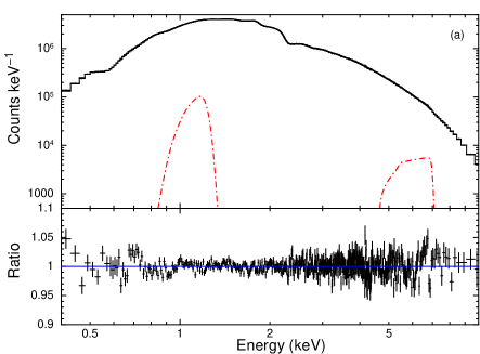
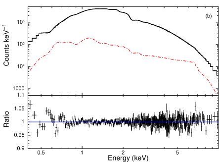
Figure 3.— Spectra of Serpens X-1 with reflection modeled using relline (a) to account for the Fe L and K lines individually and relxillNS (b) to account for entire reflection spectrum indicated by the red dot-dashed lines. The lower panels indicate the ratio of the NICER data to overall model. The continuum is modeled with an absorbed disk blackbody, single temperature blackbody, and power-law component. For plotting purposes, the data were rebinned

There are two strong emission features near $1.1$ and $6.7$ keV that can be attributed to a blend of Fe L and Fe K shell emission (see Figure 1). As a consistency check, we overplot the NuSTAR and XMM-Newton ratio-to-continuum spectra in the lower panel of Figure 1. The presence of these features in other detectors verifies that they are not due to the NICER instrumentation. We initially apply Gaussian profiles to each feature, which improves the fit by $\Delta\chi^{2}=290$ for six degrees of freedom. The low-energy emission feature has a line centroid energy of $1.12\pm 0.01$ keV with width $\sigma=0.10_{-0.01}^{+0.02}$ keV and normalization of $9.8\pm 0.2\times 10^{-3}$ photons cm^-2 s^-1, which is similar to the values reported in Cackett et al. (2010) for the XMM-Newton/PN data. We again checked that the low-energy feature is not an instrumental artifact by fixing the width of the line to 0, which is a delta function in xspec and indicates the resolution of the detector. We find that a line width of zero is ruled out at $9\sigma$, corroborating that the line is not native to the instrumentation. The Fe K emission feature has a line centroid energy of $6.59\pm 0.04$ keV with width $\sigma=0.26_{-0.05}^{+0.06}$ keV and normalization of $3.8\pm 0.1\times 10^{-3}$ photons cm^-2 s^-1. The equivalent widths of the Fe K and Fe L lines are $0.064\pm 0.002$ keV and $0.0090\pm 0.0001$ keV, respectively. The equivalent width of the Fe K line is comparable to values reported in Cackett et al. (2010) for XMM-Newton and Suzaku observations of other NS LMXBs, whereas the Fe L blend agrees with Vrtilek et al. (1988).

Table 1Reflection Modeling of Ser X-1

Model	Parameter	relline	relxillNS
tbnew	$\mathrm{N}_{\mathrm{H}}$ ($10^{21}$ cm-2)	$6.9\pm 0.1$	$6.38\pm 0.02$
	$A_{O}$	$1.10\pm 0.01$	$1.25_{-0.05}^{+0.02}$
	$A_{Fe}$	$1.12_{-0.02}^{+0.09}$	$0.88_{-0.04}^{+0.09}$
diskbb	kT (keV)	$1.13_{-0.02}^{+0.03}$	$1.15_{-0.02}^{+0.05}$
	norm	$130_{-20}^{+10}$	$120_{-10}^{+3}$
bbody	kT (keV)	$1.80\pm 0.02$	$1.85_{-0.03}^{+0.11}$
	K ($10^{-2}$)	$4.9\pm 0.2$	$3.1_{-0.4}^{+0.6}$
powerlaw	$\Gamma$	$2.5\pm 0.1$	$1.8_{-0.1}^{+0.5}$
	norm ($10^{-1}$)	$5.0_{-0.4}^{+0.7}$	$3.50\pm 0.04$
relline1	LineE (keV)	$6.96_{-0.07}^{+0.01}$	…
	$q$	$3.00_{-0.16}^{+0.08}$	…
	$i$ (∘)	$10.1_{-0.2}^{+4.9}$	…
	$R_{in}$ ($R_{\mathrm{ISCO}}$)	$1.03_{-0.03}^{+0.13}$	…
	$R_{in}$ ($R_{g}$)	$6.2_{-0.2}^{+0.8}$	…
	$R_{in}$ (km)	$12.7_{-0.4}^{+1.6}$	…
	norm ($10^{-3}$)	$7.1_{-1.0}^{+0.9}$	…
relline2	LineE (keV)	$1.22_{-0.02}^{+0.01}$	…
	$R_{in}$ ($R_{\mathrm{ISCO}}$)	$1.4_{-0.1}^{+0.2}$	…
	$R_{in}$ ($R_{g}$)	$8.4_{-0.6}^{+1.2}$	…
	$R_{in}$ (km)	$17.3_{-1.2}^{+2.5}$	…
	norm ($10^{-3}$)	$6.8_{-0.7}^{+1.2}$	…
relxillNS	$q$	…	$2.51_{-0.17}^{+0.04}$
	$i$ (∘)	…	$4.43_{-0.30}^{+0.01}$
	$R_{in}$ ($R_{\mathrm{ISCO}}$)	…	$1.18_{-0.02}^{+0.10}$
	$R_{in}$ ($R_{g}$)	…	$7.08_{-0.12}^{+0.60}$
	$R_{in}$ (km)	…	$14.6_{-0.3}^{+1.2}$
	$\log\xi$	…	$3.2\pm 0.1$
	$A_{Fe}$	…	$4.8_{-0.3}^{+0.8}$
	$\log N$ (cm-3)	…	$18.83\pm 0.04$
	$f_{\mathrm{refl}}$ ($10^{-1}$)	…	$5.4_{-0.7}^{+0.3}$
	norm ($10^{-3}$)	…	$1.4\pm 0.3$
	Funabs	$10\pm 3$	$9\pm 3$
	$\chi^{2}$ (d.o.f.)	1232.9 (942)	1180.4 (942)

Note.— Errors are reported at the 90% confidence level and calculated from Markov chain Monte Carlo (MCMC) of chain length 500,000. The emissivity index $q$ and inclination $i$ were tied between relline components, and the line emission is assumed to be isotropic. The outer disk radius was fixed at 990 $R_{g}$, the dimensionless spin parameter and redshift were set to zero for both the relline and relxillNS models. The temperature of the blackbody in the relxillNS model was linked to the single temperature blackbody of the continuum. The relxillNS model was set to reflection only and $f_{\mathrm{refl}}$ denotes the reflection fraction. The unabsorbed flux is taken in the $0.4-10.0$ keV band and given in units of $10^{-9}$ ergs s^-1 cm^-2. For reference, for $a=0$ and canonical NS mass $M_{\mathrm{NS}}=1.4\ M_{\odot}$, $1\ R_{\mathrm{ISCO}}=6\ R_{g}=12.4$ km.

As a further refinement, we replace the Gaussian line components with the relativistic reflection line model relline (Dauser et al., 2010). We fixed the spin parameter, $a=cJ/GM^{2}$, to $a=0$ since most NS in LMXBs have $a\leq 0.3$ (Galloway et al. 2008; Miller 2011). The choice of spin does not have a strong impact on our results; the difference in position of the $R_{\mathrm{ISCO}}$ between $a=0.0$ and $a=0.3$ is less than 1 $R_{g}$ (where $R_{g}=GM/c^{2}$). We allowed the inner disk radii to be independent for each line component but tied the inclination and emissivity index between the lines. The outer disk radius was fixed to 990 $R_{g}$ in each case. The double relativistic reflection provides a $10\sigma$ improvement in the overall fit, although a Gaussian line cannot be statistically ruled out for the Fe L complex. We find $R_{in}$ of $1.4_{-0.1}^{+0.2}$ $R_{\mathrm{ISCO}}$ for Fe L and $1.03_{-0.03}^{+0.13}$ $R_{\mathrm{ISCO}}$ for Fe K. Additionally, the inclination of $10.1_{-0.2}^{+4.9}$ degrees from these lines agrees with the early NuSTAR results (Miller et al., 2013) and optical spectroscopy (Cornelisse et al., 2013). Table 1 reports the values of all free parameters. Figure 3(a) shows the ratio of the data to the overall fit as well as the relline model components. The increase in line energy for the Fe L feature is due to the relline model interpreting the feature as a single line rather than a complex of lines between 0.9 to 1.3 keV. There are still residuals in the $6-7$ keV energy band suggesting that relline is unable to fully account for the Fe K line, hence we proceed with applying a self-consistent reflection model.

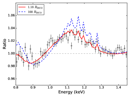
Figure 4.— Best-fit reflection model reported in Table 1 at 1.18 $R_{\mathrm{ISCO}}$ (red) and contrasting 100 $R_{\mathrm{ISCO}}$ (blue) overlaid on the NICER data to highlight the broad Fe L shell blend between 0.9 and 1.3 keV. The larger inner disk radius relaxes the relativistic effects to show the narrow emission lines in that region, likely due to Mg III-VII. The data were rebinned for clarity.

To obtain a more physical description of these features, we employ a preliminary version of the fully self-consistent reflection model, relxillNS, which computes illumination of the disk by a blackbody spectrum (rather than the power-law input of the original relxill model, García et al. 2014). The model allows for the input blackbody temperature $kT_{bb}$, log of the ionization parameter $\log\xi$, iron abundance $A_{Fe}$, and log of the density of the disk $\log(N$ [cm^-3]$)$. All other elements are hard-coded to solar abundance. In order for the model to pick up both the Fe L blend and Fe K line, the disk requires a high density and $\sim 5$ times solar iron abundance (see García et al. 2016 and Ludlam et al. 2017 for discussion of disk density and iron abundance). This fit is reported in Table 1. Figure 3(b) shows the ratio of the data to the model as well as the reflection component. In Figure 4 we plot the reflection model in the region of the low-energy feature to demonstrate the blending of the Fe L shell transitions. In order to illustrate the local-frame emission spectrum, which better shows the line complex features, we set $R_{in}$ to 100 $R_{\mathrm{ISCO}}$, a value so large as to effectively remove relativistic distortions. The narrow emission lines in the same region as the broad Fe  L shell are likely due to a lower-Z element such as Mg III–VII.

The single inner disk radius inferred from the relxillNS fit falls between the radii obtained from the Fe K line and Fe L blend in the relline fit. This could be due to the model applying the same physical conditions to each line when they could be arising from different locations and/or ionizations within the disk. We currently lack the data quality needed for a double relxillNS fit to explore multiple ionization zones.

4. Discussion

Through the sensitivity and passband of NICER we detected a broad Fe L blend and Fe K in the persistent emission of Ser X-1. We confirm that these lines are not native to NICER instrumentation by comparing the spectra to observations made by NuSTAR and XMM-Newton/RGS. NICER captures $\sim 1.34\times 10^{6}$ photons in the Fe L band and $\sim 2.75\times 10^{5}$ photons in the Fe K band in just 4.5 ks. These lower-energy Fe L lines have the potential to improve the statistical power of disk reflection and, ultimately, can be a very important tool for placing constraining upper limits on the radii of neutron stars if the lines indeed arise from the innermost regions of accretion disks. The position of the inner disk radius inferred from the Fe L blend ($1.4_{-0.1}^{+0.2}$ $R_{\mathrm{ISCO}}$) is consistent with the value inferred from the Fe K line ($1.03_{-0.03}^{+0.13}$ $R_{\mathrm{ISCO}}$) within the joint $3\sigma$ uncertainties. This is similar to the inner disk radius implied by the diskbb normalization of the best fit model ($\sim 21-28$ km) for an inclination of $10^{\circ}$, distance of $7.7\pm 0.9$ kpc (Galloway et al., 2008), and color correction factor of 1.7 (Kubota et al., 1998). Our results for the position of the inner disk agree with previous spectral studies that utilize data from different observatories, such as Suzaku, Chandra, XMM-Newton, and NuSTAR (Bhattacharyya & Strohmayer 2007; Cackett et al. 2008, 2010; Chiang et al. 2016; Miller et al. 2013).

Furthermore, we demonstrate that both the low-energy blend and Fe K line can be modeled with self-consistent reflection, but we are at the limits of the current data set. As the mission progresses and calibration is improved, we will gain a larger sample of data from which we can explore a double relxillNS model to determine the locations of these features individually and potentially explore the ionization structure of the disk (Ludlam et al., 2016). In a forthcoming paper, a final version of relxillNS will be described and applied to a larger set of NICER data, with the goal of further enhancing our understanding of the innermost disk around neutron stars.

References

- Arnaud (1996) Arnaud, K. A. 1996, in Astronomical Society of the Pacific Conference Series, Vol. 101, Astronomical Data Analysis Software and Systems V, ed. G. H. Jacoby & J. Barnes, 17
- Bhattacharyya & Strohmayer (2007) Bhattacharyya, S., & Strohmayer, T. 2007, ApJ, 664, 103
- Cackett et al. (2008) Cackett, E. M., Miller, J. M., Bhattacharyya, S., Grindlay, J. E., Homan, J., van der Klis, M., Miller, M. C., Strohmayer, T. E., & Wijnands, R. 2008, ApJ, 674, 415
- Cackett et al. (2010) Cackett, E. M., Miller, J. M., Ballantyne, D. R., Barret, D., Bhattacharyya, S., Boutelier, M., Coleman Miller, M. Strohmayer, T. E., & Wijnands, R. 2010, ApJ, 720, 205
- Chiang et al. (2016) Chiang, C.-Y., Cackett, E. M., Miller, J. M., et al. 2016, ApJ, 821, 105
- Cornelisse et al. (2013) Cornelisse, R., Casares, J., Charles, P. A., & Steeghs, D. 2013, MNRAS, 432, 1361
- Dauser et al. (2010) Dauser, T., Wilms, J., Reynolds, C. S., & Brenneman, L. W. 2010, MNRAS, 409, 1534
- Degenaar et al. (2018) Degenaar, N., Ballantyne, D. R., Belloni, T., et al. 2018, SSRv, 214, 15
- Dickey & Lockman (1990) Dickey, J. M., & Lockman, F. J. 1990, ARA&A, 28, 215
- Fabian et al. (1989) Fabian, A. C., Rees, M. J., Stella, L., & White, N. E. 1989, MNRAS, 238, 729
- Fabian et al. (2009) Fabian, A. C., Zoghbi, A., Ross, R. R., et al. 2009, Nat, 459, 540
- Galloway et al. (2008) Galloway, D. K., Muno, M. P., Hartman, J. M., Psaltis, D., & Chakrabarty, D. 2008, ApJS, 179, 360
- García et al. (2014) García, J., Dauser, T., Lohfink, A., et al. 2014, ApJ, 782, 76
- García et al. (2016) García, J., Fabian, A. C., Kallman, T. R., et al. 2016, MNRAS, 462, 751
- Gendreau et al. (2012) Gendreau, K. C., Arzoumanian, Z., & Okajima, T. 2012, in Society of Photo-Optical Instrumentation Engineers (SPIE) Conference Series, Vol. 8443, 13
- Iaria et al. (2009) Iaria, R., D’aì, A., Di Salvo, T., et al. 2009, A&A, 505, 1143
- Jahoda et al. (2006) Jahoda, K., Markwardt, C. B., Radeva, Y., et al. 2006, ApJS, 163, 401
- Kubota et al. (1998) Kubota, A., Tanaka, Y., Makishima, K., et al. 1998, PASJ, 50, 667
- Kuulkers et al. (1997) Kuulkers, E., Parmar, A. N., Owens, A., Oosterbroek, T., & Lammers, U. 1997, A&A, 323, L29
- Lin et al. (2007) Lin, D., Remillard, R. A., & Homan, J. 2007, ApJ, 667, 1073
- Ludlam et al. (2017) Ludlam, R. M., Miller, J. M., Bachetti, M., et al. 2017, ApJ, 836, 140
- Ludlam et al. (2016) Ludlam, R. M., Miller, J. M., Cackett, E. M., et al. 2016, ApJ, 824, 37
- Matranga et al. (2017) Matranga, M., Di Salvo, T., Iaria, R., et al. 2017, A&A, 600, 24
- Miller (2002) Miller, J. M., Fabian, A. C., Reynolds, C. S., et al. 2002, AAS, 201, 5701
- Miller (2007) Miller, J. M. 2007, ARA&A, 45, 441
- Miller (2011) Miller, J. M., Maitra, D., Cackett, E. M., Bhattacharyya, S., & Strohmayer, T. E. 2011, ApJ, 731, L7
- Miller et al. (2013) Miller, J. M., Parker, M. L., Fuerst, F., et al. 2013, ApJ, 779, L2
- Ng et al. (2010) Ng, C., Díaz Trigo, M., Cadolle Bel, M., & Migliari, S. 2010, A&A, 522, 96
- Ponti et al. (2010) Ponti, G., Gallo, L. C., Fabian, A. C., et al. 2010, MNRAS, 406, 2591
- Popham & Sunyaev (2001) Popham, R., & Sunyaev, R. 2001, ApJ, 547, 355
- Sidoli et al. (2001) Sidoli, L., Oosterbroek, T., Parmar, A. N., Lumb, D., & Erd, C. 2001, A&A, 379, 540
- Schulz (1999) Schulz, N. S. 1999, ApJ, 511, 304
- Sunyaev et al. (1991) Sunyaev, R. A., Arefev, V. A., Borozdin, K. N., et al. 1991, Soviet Astronomy Letters, 17, 409
- Verner et al. (1996) Verner, D. A., Ferland, G. J., Korista, K. T., & Yakovlev, D. G. 1996, ApJ, 465, 487
- Vrtilek et al. (1988) Vrtilek, S. D., Swank, J. H., & Kallman, T. R. 1988, ApJ, 326, 186
- Weisskopf et al. (2010) Weisskopf, M.C., Guainazzi, M., Jahoda, K., et al. 2010, ApJ, 713, 912
- Wilms et al. (2000) Wilms, J., Allen, A., & McCray, R. 2000, ApJ, 542, 914