Communication over an Arbitrarily Varying Channel under a State-Myopic Encoder

Abstract

We study the problem of communication over a discrete arbitrarily varying channel (AVC) when a noisy version of the state is known non-causally at the encoder. The state is chosen by an adversary which knows the coding scheme. A state-myopic encoder observes this state non-causally, though imperfectly, through a noisy discrete memoryless channel (DMC). We first characterize the capacity of this state-dependent channel when the encoder-decoder share randomness unknown to the adversary, i.e., the randomized coding capacity. Next, we show that when only the encoder is allowed to randomize, the capacity remains unchanged when positive. Interesting and well-known special cases of the state-myopic encoder model are also presented.

I Introduction

Consider the communication setup in Fig. 1, where a message $M$ is sought to be transmitted over a memoryless state-dependent channel $W_{Y|X,S}$.

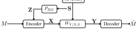
Figure 1: The communication setup

The channel state is controlled by a jamming adversary which knows the coding scheme and can input arbitrary state vectors $\mathbf{S}$, possibly through randomized strategies. The adversary’s choice of state $\mathbf{S}$ is revealed non-causally, though imperfectly, to the encoder. In particular, we assume that along with $M$, the encoder has a noisy or myopic view $\mathbf{Z}$ of state $\mathbf{S}$, where $\mathbf{S}$ is observed through a discrete memoryless channel (DMC) $P_{Z|S}$. In this work, we study the capacity of this state-dependent channel under a state-myopic encoder.

State-dependent channels, especially discrete channels which are the focus in the work, have received considerable attention in literature. For such channels, the capacity under non-causal awareness of the state at the encoder, when components of the random state are generated according to a known independent and identically distributed (i.i.d.) process, was characterized in the seminal work of Gel’fand and Pinsker [2] (see also [3]). Cover and Chiang [4] characterized the capacity when the encoder’s non-causal view was corrupted via a noisy DMC (see also [5] for a simpler proof). Versions of each of these problems under causal knowledge of state have also appeared (cf. [6, 7, 8]).

Ahlswede [9] analysed an adversarial version of this Gel’fand-Pinsker problem [2], where the channel state $\mathbf{S}$ may be chosen arbitrarily. Several other closely related adversarial channel models (see, for instance, [10, 11, 12, 13] and some of the references therein) have subsequently been studied. More generally, all of these channels belong to the class of arbitrarily varying channels (AVC), first proposed in [14]. The AVC framework has subsequently been employed extensively to study varied adversarial communication problems. It is well known (cf. [15, 16]) that the nature of results for AVCs crucially depend upon the assumptions made with respect to (w.r.t.) the communication system, for instance, the knowledge/capabilities possessed by the adversary and/or user. Adversary models have, in particular, received considerable attention. Several models have appeared, ranging from a ‘blind’ or oblivious adversary with no knowledge of the codeword (e.g. [14, 17, 18]) to an omniscient adversary with a perfect knowledge of the codeword (e.g. [19, 20]). More generally, a myopic adversary with a noisy view of the codeword was studied in [1] under randomized coding. A sufficiently myopic adversary model, where the adversary’s view is more noisy than the level of channel noise it can hope to induce, was recently considered in [21].

In this work, reversing the gaze from the adversary to the user, we study the impact of myopicity at the encoder vis-à-vis the adversary’s jamming state. Our state-myopic encoder model can be viewed as a bridge connecting Ahlswede’s state-omniscient model [9] with zero or no state-myopicity (i.e., under a full-rate observation channel) to the state-oblivious model in [14, 17, 18] with full state-myopicity (i.e., under a zero-rate observation channel). We refine this view through our main results. We first characterize the randomized coding capacity. Towards upper bounding the rate, our converse uses a memoryless, but crucially, a non-identically distributed jamming strategy which may depend on the code. Our proof of achievability uses the approach in [12], and employs a refined Markov lemma [12]. This approach is different from the two-step approach in [9] which entails first studying a compound channel version (only memoryless jamming strategies permissible) of the problem, followed by determining the randomized coding capacity using the ‘robustification technique’ [9, pg. 625]. We then show that when only the encoder can privately randomize, the capacity remains unchanged when non-zero.

The rest of the paper is organized as follows. We introduce the notation and the problem setup in Section II. The main results are stated in Section III, while their proofs are presented in Section IV. We discuss some implications of our results, in particular, we elaborate upon aforementioned connections to well-known problems, and make concluding remarks in Section V.

II Notation and Problem Setup

II-A Notation

Let us denote random variables by upper case letters (e.g. $X$), the values they take by lower case letters (e.g. $x$) and their alphabets by calligraphic letters (e.g. $\mathcal{X}$). We use the boldface notation to denote random vectors (e.g. $\mathbf{X}$) and their values (e.g. $\mathbf{x}$). Here the vectors are of length $n$ (e.g. $\mathbf{X}=(X_{1},X_{2},\dots,X_{n})$), where $n$ is the block length of operation. Let $\mathbf{X}^{i}=(X_{1},X_{2},\dots,X_{i})$ and $\mathbf{x}^{i}=(x_{1},x_{2},\dots,x_{i})$ as well as $\mathbf{X}_{i}^{k}=(X_{i},X_{i+1},\dots,X_{k})$ and $\mathbf{x}_{i}^{k}=(x_{i},x_{i+1},\dots,x_{k})$. We use the $l_{\infty}$ norm denoted by $\|.\|_{\infty}$ for discrete vectors. For a set $\mathcal{X}$, let ${\cal P}(\mathcal{X})$ be the set of all probability distributions on $\mathcal{X}$. Similarly, let us write as ${\cal P}(\mathcal{X}|\mathcal{Y})$, the set of all conditional distributions of a random variable with alphabet $\mathcal{X}$ conditioned on another random variable with alphabet $\mathcal{Y}$. Let $X$ and $Y$ be two random variables. Then, we denote the distribution of $X$ by $P_{X}(\cdot)$, the joint distribution of $(X,Y)$ by $P_{XY}(\cdot,\cdot)$ and the conditional distribution of $X$ given $Y$ by $P_{X|Y}(\cdot|\cdot)$. We denote the marginal distribution of $X$ obtained from $P_{X,Y}$ by $[P_{X,Y}]_{X}$. Distributions corresponding to strategies adopted by the adversary are denoted by $Q$ instead of $P$ for clarity. Functions will be denoted in lowercase letters (e.g., $f$). We denote a type of $X$ by $T_{X}$. Given sequences $\mathbf{x}$, $\mathbf{y}$, we denote by $T_{\mathbf{x}}$ the type of $\mathbf{x}$, by $T_{\mathbf{x},\mathbf{y}}$ the joint type of $(\mathbf{x},\mathbf{y})$ and by $T_{\mathbf{x}|\mathbf{y}}$ the conditional type of $\mathbf{x}$ given $\mathbf{y}$. For $\epsilon\in(0,1)$, the set of $\epsilon$-typical sequences $\mathbf{x}$ for a distribution $P_{X}$ is $\mathcal{T}^{n}_{\epsilon}(P_{X})=\{\mathbf{x}:\|T_{\mathbf{x}}-P_{X}\|_{\infty}\leq\epsilon\},$ and for a joint distribution $P_{X,Y}$ and $\mathbf{x}\in{\cal X}^{n}$, the set of conditionally $\epsilon$-typical set of sequences $\mathbf{y}$, conditioned on $\mathbf{x}$, is defined as $\mathcal{T}^{n}_{\epsilon}(P_{X,Y}|\mathbf{x})=\{\mathbf{y}:\|T_{\mathbf{x},\mathbf{y}}-P_{X,Y}\|_{\infty}\leq\epsilon\}.$

II-B Problem Setup

As shown in Fig. 1, a message $M$ is sent over an AVC with user input $X$, jamming state $S$ and channel output $Y$. Random variables $X$, $S$ and $Y$ take values in finite sets ${\cal X}$, ${\cal S}$ and ${\cal Y}$ respectively. The channel behaviour is given by the fixed distribution $W_{Y|X,S}$. We consider the standard block coding framework with block length $n$, where $X_{i}$, $S_{i}$ and $Y_{i}$ denote the symbols associated with the $i$-th time instant. The jamming state $\mathbf{S}$ is chosen by the adversary. Let $Q_{\mathbf{S}}$ denote its distribution, which is arbitrary and unknown to user. A state-myopic encoder receives two inputs: message $M$ and a noisy and non-causal version $\mathbf{Z}$ of the state $\mathbf{S}$. Here $\mathbf{Z}$, where $Z_{i}\in{\cal Z}$, $\forall i$ and $|{\cal Z}|<\infty$, is output by a fixed DMC $P_{Z|S}$ under input $\mathbf{S}$. The encoder transmits $\mathbf{X}$ on the channel. Upon receiving its noisy version $\mathbf{Y}$, the decoder outputs an estimate $\tilde{M}$ of the message $M$.

An $(n,R)$ deterministic code of block length $n$ and rate $R$ consists of a deterministic encoder-decoder pair $(\psi,\phi)$, where $\psi:\{1,2,\dots,2^{nR}\}\times{\mathcal{Z}}^{n}\rightarrow{\mathcal{X}}^{n}$ and decoder $\phi:{\mathcal{Y}}^{n}\rightarrow\{0,1,2,\dots,2^{nR}\}$, where an output of $0$ indicates decoding error. We assume that $2^{nR}$ is an integer. An $(n,R)$ randomized code of block length $n$ and rate $R$ is a random variable (denoted by $\Theta$) which takes values in the set of $(n,R)$ deterministic codes. For an $(n,R)$ randomized code, the maximum probability of error is given by $P_{e}^{(n)}:=\max_{m}\max_{Q_{\mathbf{S}}}\mathbb{P}(\phi(\mathbf{Y})\neq m|M=m),$ where the probability is evaluated over the AVC $W_{Y|X,S}$, the channel $P_{Z|S}$, the shared randomness $\Theta$ and adversary’s action. A rate $R$ is achievable if for any $\epsilon>0$, there exists an $n_{0}(\epsilon)$ large enough such that for all $n\geq n_{0}(\epsilon)$ there exist $(n,R)$ randomized codes with corresponding $P_{e}^{(n)}$ less than $\epsilon$. We define the capacity as the supremum of all achievable rates. An $(n,R)$ code with stochastic encoder of block length $n$ and rate $R$ consists of a stochastic encoder-deterministic decoder pair $(\Psi,\phi)$, where $\Psi:\{1,2,\dots,2^{nR}\}\times{\cal Z}^{n}\rightarrow{\cal P}({\cal X}^{n})$ and $\phi:{\cal Y}^{n}\rightarrow\{0,1,2,\dots,2^{nR}\}$. Here an output of $0$ indicates a decoding error. For an $(n,R)$ code with stochastic encoder, the maximum probability of error is given by $P_{e}^{(n)}:=\max_{m}\max_{Q_{\mathbf{S}}}\mathbb{P}(\phi(\mathbf{Y})\neq m|M=m).$ Here the probability is evaluated over the AVC $W_{Y|X,S}$, the channel $P_{Z|S}$, the encoding map and the adversary’s action. The definitions of achievable rate and capacity under codes with stochastic encoder can be analogously stated as earlier.

III The Main Results

We now present our main results. Define the set ${\cal P}^{Q}({\cal Z}):=\{P_{Z}\in{\cal P}({\cal Z}):P_{Z}=[Q_{S}P_{Z|S}]_{Z},Q_{S}\in{\cal P}({\cal S})\}$. Given $P_{Z}\in{\cal P}^{Q}({\cal Z})$ and some $Q_{S}\in{\cal P}({\cal S})$, where $[P_{Z|S}Q_{S}]_{Z}=P_{Z}$, and under fixed distribution $P_{U|Z}$ and function $x:{\cal U}\times{\cal Z}\rightarrow{\cal X}$, let $I(U;Y)-I(U;Z)$ denote the mutual information quantity evaluated under the joint distribution $Q_{S}P_{Z|S}P_{U|Z}\mathbf{1}_{\{X=x(U,Z)\}}W_{Y|X,S}$. Let ${\cal U}$ denote the alphabet of $U$. We define

$$C^{*}:=\min_{P_{Z}\in{\cal P}^{Q}({\cal Z})}\max_{P_{U|Z},\ x(\cdot,\cdot)}\min_{\begin{subarray}{c}Q_{S}:\\ [Q_{S}P_{Z|S}]_{Z}=P_{Z}\end{subarray}}I(U;Y)-I(U;Z),$$ (1)

where $P_{U|Z}\in{\cal P}(\mathcal{U}|{\cal Z})$, $x:{\cal U}\times{\cal Z}\rightarrow{\cal X}$ and $|{\cal U}|\leq|{\cal X}|^{|{\cal Z}|}$. We now state our first result.

Theorem 1.

The randomized coding capacity $C_{r}$ under maximum probability of error criterion is

$$C_{r}=C^{*}.$$ (2)

The proof of this result is presented in Section IV.

Theorem 2.

The capacity $C_{s}$ for codes with stochastic encoder equals the randomized coding capacity when positive.

The proof of this result can be found in Section IV.
Remarks:
1 . Although our results are stated under a maximum (over messages) probability of error criterion, they continue to hold under an average (over messages) probability of error criterion as well. This is because while the achievability is proved under the maximum probability of error criterion, our converse is proved under an average probability error of criterion.
2. Our state-myopic encoder model generalizes, through the degree of myopicity, the fully state-myopic model [14] as well as the zero state-myopic model [9]. Refer the discussion in Section V for details.

IV Proofs

IV-A Proof of Theorem 1

We first present the converse followed by the achievability.

IV-A1 Converse

Our proof for the converse considers an average probability of error criterion instead of the maximum probability of error criterion. For this stronger version of the converse, let the average probability of error be

$$P^{(n)}_{e}:=\frac{1}{2^{nR}}\sum_{m=1}^{2^{nR}}P^{(n)}_{e,m},$$

where

$$P^{(n)}_{e,m}=\max_{Q_{\mathbf{S}}}\mathbb{P}\left(\Phi(\mathbf{Y})\neq m|M=m\right).$$

Our converse will consider a specific memoryless, but possibly non-identically distributed, jamming strategy which depends on the randomized code. Under such a jamming strategy, we will upper bound the rate of reliable communication possible.

Our proof of the converse starts along the lines of the converse for the standard Gel’fand-Pinsker problem [22]. Consider any sequence of randomized $(n,R)$ codes with average probability of error $P_{e}^{(n)}\rightarrow 0$ as $n\rightarrow\infty$. From Fano’s inequality, we know that for such a sequence of codes $H(M|\mathbf{Y},\Theta)\leq n\epsilon_{n}$, where $\epsilon_{n}\rightarrow 0$ as $n\rightarrow\infty$.

$$nR \leq H(M)$$

$$= I(M;\mathbf{Y},\Theta)+H(M|\mathbf{Y},\Theta)$$

$$\leq I(M;\mathbf{Y},\Theta)+n\epsilon_{n}$$

$$= I(M;\Theta)+I(M;\mathbf{Y}|\Theta)+n\epsilon_{n}$$

$$\stackrel{{\scriptstyle(a)}}{{=}} \sum_{i=1}^{n}I(M;Y_{i}|\mathbf{Y}^{i-1},\Theta)+n\epsilon_{n}$$

$$\leq \sum_{i=1}^{n}I(M,\mathbf{Y}^{i-1},\Theta;Y_{i})+n\epsilon_{n}$$

$$= \sum_{i=1}^{n}I(M,\mathbf{Z}_{i+1}^{n},\mathbf{Y}^{i-1},\Theta;Y_{i})-\sum_{i=1}^{n}I(Y_{i};Z_{i+1}^{n}|M,\mathbf{Y}^{i-1},\Theta)+n\epsilon_{n}$$

$$\stackrel{{\scriptstyle(b)}}{{=}} \sum_{i=1}^{n}I(M,\mathbf{Z}_{i+1}^{n},\mathbf{Y}^{i-1},\Theta;Y_{i})-\sum_{i=1}^{n}I(\mathbf{Y}^{i-1};Z_{i}|M,\mathbf{Z}_{i+1}^{n}\Theta,)+n\epsilon_{n}$$

$$\stackrel{{\scriptstyle(c)}}{{=}} \sum_{i=1}^{n}I(M,\mathbf{Z}_{i+1}^{n},\mathbf{Y}^{i-1},\Theta;Y_{i})-\sum_{i=1}^{n}I(M,\mathbf{Z}_{i+1}^{n},\mathbf{Y}^{i-1},\Theta;Z_{i})+n\epsilon_{n}$$

$$\stackrel{{\scriptstyle(d)}}{{=}} \sum_{i=1}^{n}I(U_{i};Y_{i})-\sum_{i=1}^{n}I(U_{i};Z_{i})+n\epsilon_{n}$$

$$\stackrel{{\scriptstyle}}{{=}} n\left(\sum_{i=1}^{n}\frac{1}{n}\left(I(U_{i};Y_{i})-I(U_{i};Z_{i})\right)\right)+n\epsilon_{n}.\yesnumber$$

We get $(a)$ via the independence of $M$ and $\Theta$, while $(b)$ follows from Csiszár’s sum identity [22, pg. 25]. Under memoryless jamming, $Z_{i}$ is independent of $(M,\mathbf{Z}_{i+1}^{n},\Theta)$, $\forall i$, which gives us $(c)$. By introducing the auxiliary variable $U_{i}:=(M,\mathbf{Z}_{i+1}^{n},\mathbf{Y}^{i-1},\Theta)$, $\forall i$, we have $(d)$.

Although the adversary can employ arbitrary jamming strategies $Q_{\mathbf{S}}$, we analyse the rate performance under memoryless jamming strategies. In particular, given a randomized encoding map, let us assume that the adversary restricts to only memoryless (though, possibly non-identically distributed) jamming strategies of the form

$$Q_{\mathbf{S}}(\mathbf{s}):=\prod_{i=1}^{n}Q_{S_{i}}(s_{i}),$$

where $Q_{S_{i}}\in{\cal P}({\cal S})$. Observe that under such memoryless jamming strategies, we have $(U_{i},Z_{i})\rightarrow(X_{i},S_{i})\rightarrow Y_{i}$, $\forall i$. Prior to specifying the jamming strategy $Q_{\mathbf{S}}$, by specifying $Q_{S_{i}}(s_{i})$ for each $i$, note that we have

$$P_{U_{i},X_{i}|Z_{i}} (U_{i}=u_{i},X_{i}=x_{i}|Z_{i}=z_{i})$$

$$\stackrel{{\scriptstyle(a)}}{{=}} P_{(M,\mathbf{Z}_{i+1}^{n},\mathbf{Y}^{i-1},\Theta),X_{i}|Z_{i}}((m,\mathbf{z}_{i+1}^{n},\mathbf{y}^{i-1},\theta),x_{i}|s_{i})$$

$$\stackrel{{\scriptstyle}}{{=}} \sum_{\mathbf{s}^{i-1},\mathbf{x}^{i-1},\mathbf{x}_{i+1}^{n},\mathbf{z}^{i-1}}P_{(M,\mathbf{Z}_{i+1}^{n},\mathbf{Y}^{i-1},\Theta),\mathbf{S}^{i-1},\mathbf{X}^{i-1},\mathbf{X}_{i+1}^{n},\mathbf{Z}^{i-1},X_{i}|Z_{i}}((m,\mathbf{z}_{i+1}^{n},\mathbf{y}^{i-1},\theta),\mathbf{s}^{i-1},\mathbf{x}^{i-1},\mathbf{x}_{i+1}^{n},\mathbf{z}^{i-1},x_{i}|z_{i})$$

$$\stackrel{{\scriptstyle}}{{=}} \sum_{\mathbf{s}^{i-1},\mathbf{x}^{i-1},\mathbf{x}_{i+1}^{n},\mathbf{z}^{i-1}}P_{M}(m)P_{\Theta}(\theta)P_{\mathbf{S}^{i-1},\mathbf{Z}^{i-1}}(\mathbf{s}^{i-1},\mathbf{z}^{i-1})P_{\mathbf{Z}_{i+1}^{n}}(\mathbf{z}_{i+1}^{n})$$

$$\hskip 71.13188pt\cdot P_{(\mathbf{X}^{i-1},X_{i},\mathbf{X}_{i+1}^{n})|M,\Theta,\mathbf{Z}}((\mathbf{x}^{i-1},x_{i},\mathbf{x}_{i+1}^{n})|m,\theta,\mathbf{z})P_{\mathbf{Y}^{i-1}|\mathbf{X}^{i-1},\mathbf{S}^{i-1}}(\mathbf{y}^{i-1}|\mathbf{x}^{i-1},\mathbf{s}^{i-1})$$

$$\stackrel{{\scriptstyle}}{{=}} \sum_{\mathbf{s}^{i-1},\mathbf{x}^{i-1},\mathbf{x}_{i+1}^{n},\mathbf{z}^{i-1}}P_{M}(m)P_{\Theta}(\theta)\left[Q_{\mathbf{S}^{i-1}}(\mathbf{s}^{i-1})P_{\mathbf{Z}^{i-1}|\mathbf{S}^{i-1}}(\mathbf{z}^{i-1}|\mathbf{s}^{i-1})\right]\left[\sum_{\mathbf{s}_{i+1}^{n}}Q_{\mathbf{S}_{i+1}^{n}}(\mathbf{s}_{i+1}^{n})P_{\mathbf{Z}_{i+1}^{n}|\mathbf{S}_{i+1}^{n}}(\mathbf{z}_{i+1}^{n}|\mathbf{s}_{i+1}^{n})\right]$$

$$\hskip 71.13188pt\cdot P_{\mathbf{X}|M,\Theta,\mathbf{Z}}(\mathbf{x}|m,\theta,\mathbf{z})P_{\mathbf{Y}^{i-1}|\mathbf{X}^{i-1},\mathbf{S}^{i-1}}(\mathbf{y}^{i-1}|\mathbf{x}^{i-1},\mathbf{s}^{i-1})$$

$$\stackrel{{\scriptstyle}}{{=}} \sum_{\mathbf{s}^{i-1},\mathbf{x}^{i-1},\mathbf{x}_{i+1}^{n},\mathbf{z}^{i-1}}P_{M}(m)P_{\Theta}(\theta)\left[\prod_{j=1}^{i-1}Q_{S_{j}}(s_{j})P_{Z|S}(z_{j}|s_{j})\right]\left[\sum_{\mathbf{s}_{i+1}^{n}}\left(\prod_{j=i+1}^{n}Q_{S_{j}}(s_{j})P_{Z|S}(z_{j}|s_{j})\right)\right]$$

$$\hskip 71.13188pt\cdot P_{\mathbf{X}|M,\Theta,\mathbf{Z}}(\mathbf{x}|m,\theta,\mathbf{z})\left[\prod_{j=1}^{i-1}W_{Y|X,S}(y_{j}|x_{j},s_{j})\right].\yesnumber$$

Here $(a)$ follows from substituting $U_{i}=(M,\mathbf{Z}_{i+1}^{n},\mathbf{Y}^{i-1},\Theta)$ and $u_{i}=(m,\mathbf{z}_{i+1}^{n},\mathbf{y}^{i-1},\theta)$. From (IV-A1), it follows that $P_{U_{i},X_{i}|Z_{i}}$ depends on $\{Q_{S_{i}}\}_{i=1}^{n}$. In particular, given $U_{i}=(M,\Theta,\mathbf{Z}_{i+1}^{n},\mathbf{Y}^{i-1})$, this dependence on the jamming strategy $Q_{\mathbf{S}}$ is captured in a two-fold manner: dependence on all past outputs $\mathbf{Y}^{i-1}$ (depends on $Q_{\mathbf{S}^{i-1}}$), and dependence on all future noisy observations $\mathbf{Z}_{i+1}^{n}$ of the jamming state (depends on $Q_{\mathbf{S}_{i+1}^{n}}$) at the encoder. We now curtail this dependence to only jamming strategies of the past by further restricting the memoryless (possibly non-i.i.d.) jamming strategies $\{Q_{S_{i}}\}_{i=1}^{n}$ to those which induce a fixed i.i.d. marginal $P_{Z}\in{\cal P}^{Q}({\cal Z})$ at the encoder, i.e., $[Q_{S_{i}}P_{Z|S}]_{Z}=P_{Z_{i}}=P_{Z}$, $\forall i$, where $P_{Z}\in{\cal P}^{Q}({\cal Z})$. The effect of this restriction (cf. (IV-A1)) is that while $P_{U_{i},X_{i}|Z_{i}}$ continues to depend on the randomized encoder $P_{\mathbf{X}|M,\Theta,\mathbf{Z}}$ in the same manner, it’s dependence on the jamming strategy $Q_{\mathbf{S}}$ is only via $\{Q_{S_{j}}\}_{j=1}^{i-1}$ and the known distribution $P_{Z}$. This allows us to now define $Q_{S_{i}}$ inductively as follows. For $i=1,2,\dots,n$, given $\{Q_{S_{j}}\}_{j=1}^{i-1}$ and $P_{U_{i},X_{i}|Z_{i}}$, let

$$Q_{S_{i}}:=\operatorname*{arg\,min}_{{\tilde{Q}}_{S_{i}}:[{\tilde{Q}}_{S_{i}}P_{Z|S}]=P_{Z}}(I(U_{i};Y_{i})-I(U_{i};S_{i})).\yesnumber$$

Thus, it follows from (IV-A1) and  (IV-A1) that

$$nR \stackrel{{\scriptstyle}}{{\leq}} n\left(\sum_{i=1}^{n}\frac{1}{n}\min_{Q_{S_{i}}:[Q_{S_{i}}P_{Z|S}]_{Z}=P_{Z}}(I(U_{i};Y_{i})-\sum_{i=1}^{n}I(U_{i};Z_{i}))\right)+n\epsilon_{n}.$$

for $P_{U_{i},X_{i}|Z_{i}}$, $i=1,2,\dots,n$. Further, observe that for $i=1,2,\ldots,n$,

$$\min_{Q_{S_{i}}:[Q_{S_{i}}P_{Z|S}]_{Z}=P_{Z}}\left(I(U_{i};Y_{i})-I(U_{i};Z_{i})\right)\leq\max_{P_{U_{i},X_{i}|Z_{i}}}\min_{Q_{S_{i}}:[Q_{S_{i}}P_{Z|S}]_{Z}=P_{Z}}\left(I(U_{i};Y_{i})-I(U_{i};Z_{i})\right),$$ (3)

where the maximization is over all $P_{U_{i},X_{i}|Z_{i}}$ with finite alphabet ${\cal U}$ of $U_{i}$. Here the inequality in (3) holds as the fixed $P_{U_{i},X_{i}|Z_{i}}$ (induced by the code) on the LHS is one such distribution. Since the channel is memoryless, the RHS in (3) does not depend on $i$, and thus, we have

$$R \stackrel{{\scriptstyle}}{{\leq}} \max_{P_{U,X|Z}}\min_{Q_{S}:[Q_{S}P_{Z|S}]_{Z}=P_{Z}}\left(I(U;Y)-I(U;Z)\right)+\epsilon_{n}.$$

Recall that we had restricted the adversary to memoryless jamming strategies $Q_{\mathbf{S}}$, where $[Q_{S_{i}}P_{Z|S}]_{Z}=P_{Z}$, $\forall i$. Removing this restriction and noting that the adversary can choose any $Q_{S}\in{\cal P}({\cal S})$ so as to induce $P_{Z}\in{\cal P}^{Q}({\cal Z})\subseteq{\cal P}({\cal Z})$, we get

$$R \stackrel{{\scriptstyle}}{{\leq}} \min_{P_{Z}\in{\cal P}^{Q}({\cal Z})}\max_{P_{U,X|Z}}\min_{Q_{S}:[Q_{S}P_{Z|S}]_{Z}=P_{Z}}\left(I(U;Y)-I(U;Z)\right)+\epsilon_{n}.$$

As this holds for all $n$, and we have $\epsilon_{n}\rightarrow 0$ as $n\rightarrow\infty$, it follows that

$$R \stackrel{{\scriptstyle}}{{\leq}} \min_{P_{Z}\in{\cal P}^{Q}({\cal Z})}\max_{P_{U,X|Z}}\min_{Q_{S}:[Q_{S}P_{Z|S}]_{Z}=P_{Z}}\left(I(U;Y)-I(U;Z)\right).$$ (4)

We now show that instead of maximizing over $P_{U,X|Z}$, it is sufficient that the maximization in (4) is over distributions $P_{U|Z}$ and functions $x:{\cal U}\times{\cal Z}\rightarrow{\cal X}$, i.e.,

$$\min_{P_{Z}\in{\cal P}^{Q}({\cal Z})}\max_{P_{U,Z|X}}\min_{\begin{subarray}{c}Q_{S}\\ :[Q_{S}P_{Z|S}]=P_{Z}\end{subarray}}\left(I(U;Y)-I(U;Z)\right)=\min_{P_{Z}\in{\cal P}^{Q}({\cal Z})}\max_{P_{U|Z},\ x(\cdot,\cdot)}\min_{\begin{subarray}{c}Q_{S}\\ :[Q_{S}P_{Z|S}]_{Z}=P_{Z}\end{subarray}}\left(I(U;Y)-I(U;Z)\right).$$ (5)

Let us fix the optimizing distribution in ${\cal P}^{Q}({\cal Z})$, say $P^{*}_{Z}$, and the corresponding conditional distribution $P_{U|Z}$. The functional representation lemma [22, pg. 626] guarantees the existence of a random variable $W$, independent of $(U,Z)$, such that $X$ is a function of $(W,U,Z)$. Let $U^{\prime}=(U,W)$ and let its alphabet be denoted by $\mathcal{U}^{\prime}$. Then, we have $P_{U^{\prime}|Z}((u,w)|z)=P_{U|Z}(u|z)P_{W}(w)$. Let the function be denoted by $x:\mathcal{U}^{\prime}\times\mathcal{Z}\rightarrow\mathcal{X}$. Note that, as required, $(U^{\prime},Z)\rightarrow(X,S)\rightarrow Y$ is a Markov chain. We now calculate the mutual information quantities under $U^{\prime}$.

$$I(U^{\prime};Z) = I(U,W;Z)$$

$$= I(U;Z)+I(W;Z|U)$$

$$= I(U;Z),\yesnumber$$

where $W\perp\!\!\!\perp(U,Z)$ gives us the last inequality. Further, for any $Q_{S}\in{\cal P}({\cal S})$ such that $[Q_{S}P_{Z|S}]_{Z}=P_{Z}^{*}$,

$$I(U^{\prime};Y) = I(U,W;Y)$$

$$= I(U;Y)+I(W;Y|U)$$

$$\geq I(U;Y),$$

and hence,

$$\min_{Q_{S}:[Q_{S}P_{Z|S}]_{Z}=P_{Z}^{*}}I(U^{\prime};Y)\geq\min_{[Q_{S}P_{Z|S}]_{Z}=P_{Z}^{*}}I(U;Y).\yesnumber$$

It then follows from (IV-A1) and (IV-A1) that for the minimizing distribution $P_{Z}^{*}$, we have

$$\min_{[Q_{S}P_{Z|S}]_{Z}=P_{Z}^{*}}I(U;Y)-I(U;Z) \leq \min_{[Q_{S}P_{Z|S}]_{Z}=P_{Z}^{*}}I(U^{\prime};Y)-I(U^{\prime};Z).$$

Note that the LHS above is evaluated under a conditional distribution $P_{X|U,Z}$ and the RHS under the corresponding $P_{U^{\prime}|Z}$ and $x:\mathcal{U}^{\prime}\times\mathcal{Z}\rightarrow\mathcal{X}$. As the inequality holds for any $P_{X|U,Z}$, we have (5), and thus

$$R \stackrel{{\scriptstyle}}{{\leq}} \min_{P_{Z}\in{\cal P}^{Q}({\cal Z})}\max_{P_{U|Z},\ x(u,z)}\min_{\begin{subarray}{c}Q_{S}\\ :[Q_{S}P_{Z|S}]_{Z}=P_{Z}\end{subarray}}\left(I(U;Y)-I(U;Z)\right).$$ (6)

Finally, the Shannon strategy approach (see, for instance, [22, Remark 7.6]) gives us the bound on the cardinality of $|{\cal U}|$. The maximization over functions $x(u,z)$ in (6) can be equivalently viewed as a maximization over the set of all functions $x_{u}:{\cal Z}\rightarrow{\cal X};u\in{\cal U}$. As exactly $|{\cal X}|^{|{\cal Z}|}$ such distinct functions exist, without loss of generality, we can restrict ${\cal U}$ to be of cardinality at most $|{\cal X}|^{|{\cal Z}|}$. This completes the proof of the converse.

IV-A2 Achievability

We provide an outline of the proof of achievability. Our outline includes a brief description of the randomized code followed by an overview of the error analysis. The detailed proof uses the approach in [23] and can be found in Appendix A.
Code design:

• For every type $T_{Z}\in{\cal P}^{Q}({\cal Z})$, choose the optimal $P_{U|Z}$ and $x(\cdot,\cdot)$ according to (2). Now we generate $2^{nR_{U}(T_{Z})}$ i.i.d. $\mathbf{U}$ sequences, each i.i.d. $\sim P_{U}$, where $P_{U}:=\left[T_{Z}P_{U|Z}\right]_{U}$, to form the codebook ${\cal C}(T_{Z})$. Each codebook ${\cal C}(T_{Z})$ is randomly partitioned into $2^{n(R_{U}(T_{Z})-\tilde{R}(T_{Z}))}$ bins. Fix $\epsilon>0$ and define

  $$R_{U}(T_{Z}) := \min_{\begin{subarray}{c}T_{S}:[T_{S}P_{Z|S}]_{Z}\stackrel{{\scriptstyle f(\epsilon)}}{{\approx}}T_{Z}\end{subarray}}I(U;Y)-\epsilon$$

  $$\tilde{R}(T_{Z}) := I(U;Z)+\epsilon$$

  $$R(T_{Z}) := R_{U}(T_{Z})-\tilde{R}(T_{Z}),\yesnumber$$

• Our randomly generated code contains this list of binned codebooks for every $T_{Z}\in{\cal P}^{Q}({\cal Z})$, and is shared between the encoder and decoder. Through the available shared randomness $\Theta$, the encoder-decoder will jointly select one code from this ensemble and use it for communication. This process is equivalent to the code being randomly generated and then shared between the encoder and the decoder.

Encoder operations:

• The encoder knows $m$ and $\mathbf{z}$. It first calculates the type $T_{\mathbf{z}}$. Next, it identifies codebook ${\cal C}(T_{\mathbf{z}})$ and the corresponding optimal pair $(P_{U|Z},x(u,z))$ (via (2)). Within bin $m$ of the codebook ${\cal C}(T_{\mathbf{z}})$, it now checks to see if there exists any codeword $\mathbf{u}_{m,k}$, $k=1,2,\dots,2^{n\tilde{R}(T_{\mathbf{z}})}$, jointly typical with the observed $\mathbf{z}$ under the distribution $P_{U|Z}T_{\mathbf{z}}$. If so, let the chosen codeword be $\mathbf{u}$, else let $\mathbf{u}:=\mathbf{u}_{1,1}$.

• Next, it generates $\mathbf{x}$, where $x_{i}=x(u_{i},z_{i})$, $i=1,2,\dots,n$. It then sends the type $T_{\mathbf{z}}$ and $\mathbf{x}$ over the channel. As there are up to a polynomial number of types [15], for large enough $n$, the rate required to convey $T_{\mathbf{z}}$ is at most $\epsilon/2$.

• Observe that the overall rate of this coding scheme (message rate is given by the smallest rate of codebook ${\cal C}(T_{Z})$ for any type $T_{Z}\in{\cal P}^{Q}({\cal Z})$)

  $$R \leq\min_{T_{Z}\in{\cal P}^{Q}({\cal Z})}R(T_{Z})+\epsilon/2$$

  $$\stackrel{{\scriptstyle(a)}}{{=}}\min_{T_{Z}\in{\cal P}^{Q}({\cal Z})}(R_{U}(T_{Z})-\tilde{R}(T_{Z})-2\epsilon)+\epsilon/2$$

  $$\stackrel{{\scriptstyle}}{{\leq}}\min_{P_{Z}\in{\cal P}^{Q}({\cal Z})}\max_{P_{U|Z},x(.,.)}\min_{\begin{subarray}{c}Q_{S}\\ [Q_{S}P_{Z|S}]_{Z}=P_{Z}\end{subarray}}I(U;Y)-I(U;Z)$$

  $$\hskip 14.22636pt-2\epsilon+\epsilon/2+\epsilon/2$$

  $$\stackrel{{\scriptstyle}}{{=}}C-\epsilon.$$

  where $(a)$ follows from (• ‣ IV-A2).

Decoder operations:

• The decoder knows $T_{\mathbf{z}}$ and observes channel output $\mathbf{y}$. It first identifies the set of conditional types

  $$\mathscr{Q}^{(n)}(T_{\mathbf{z}}) :=\{T_{S}\in{\cal P}({\cal S}):[T_{S}P_{Z|S}]_{Z}\stackrel{{\scriptstyle f(\epsilon)}}{{\approx}}T_{\mathbf{z}}\}.$$

  The set $\mathscr{Q}^{(n)}(T_{\mathbf{z}})$ contains types $T_{S}$ which result in a $Z$-marginal distribution which is close to the observed type $T_{\mathbf{z}}$.

• The decoder next determines the set of codewords $\mathbf{u}$ such that $(\mathbf{u},\mathbf{y})$ are jointly typical w.r.t. the distribution $\left[T_{S}P_{Z|S}P_{U|Z}\mathbf{1}_{\{X=x(U,Z)\}}W_{Y|X,S}\right]_{U,Y}$ for some type $T_{S}\in\mathscr{Q}^{(n)}(T_{\mathbf{z}})$. If there is a unique such codeword $\mathbf{u}$, then it outputs its bin index as the message estimate. Otherwise, it outputs $\tilde{m}=0$ indicating decoding error.

Error analysis:
An error can occur for actual codeword $\mathbf{u}\in{\cal C}(T_{\mathbf{z}})$ due to (i) $\mathbf{u}$ not being decoded correctly, and (ii) some wrong codeword $\mathbf{u}^{\prime}\in{\cal C}(T_{\mathbf{z}})$ decoded incorrectly. A decoding error for the actual codeword can occur under the following cases:

• Given $m$ and $\mathbf{z}$, the encoder cannot find within codebook ${\cal C}(T_{\mathbf{z}})$ any $\mathbf{u}$ jointly typical with $\mathbf{z}$ w.r.t. the joint distribution $P_{U|Z}T_{\mathbf{z}}$. However, as the rate $\tilde{R}(T_{Z})>I_{T_{\mathbf{z}}}(U;Z)$, the probability that the encoder cannot find such a codeword $\mathbf{u}$ is exponentially small (via covering lemma [22]).

• Let $\mathbf{u}$ be the codeword chosen by the encoder. A decoding error can occur if this $\mathbf{u}$ does not satisfy the decoding condition under any jamming state $\mathbf{s}$. We show that with high probability (w.h.p.)  such a possibility is precluded. Note that $\mathbf{z}$ observed is typical w.r.t $P_{Z|S}T_{\mathbf{s}}$. In fact, the type $T_{\mathbf{z}}\in{\cal P}^{Q}({\cal Z})$ and $T_{\mathbf{z}}$ is ‘close to’ the Z-marginal $[P_{Z|S}T_{\mathbf{s}}]_{Z}$. This implies that $T_{\mathbf{s}}$ is one of the types considered by the decoder, i.e., $T_{\mathbf{s}}\in\mathscr{Q}(T_{\mathbf{z}})$. As $(\mathbf{u},\mathbf{z})$ are jointly typical according to $P_{U|Z}T_{\mathbf{z}}$, they are also jointly typical (though with a slightly larger slack) w.r.t. $P_{U|Z}[P_{Z|S}T_{\mathbf{s}}]_{Z}$. We now use a version of the refined Markov lemma [12, Lemma 8] to show that $(\mathbf{u},\mathbf{z},\mathbf{s})$ are jointly typical according to $P_{U|Z}P_{Z|S}T_{\mathbf{s}}$. As $\mathbf{x}$ is generated via function $x(U,Z)$, it follows (using a version of the conditional typicality lemma [22]) that $(\mathbf{u},\mathbf{z},\mathbf{s},\mathbf{x})$ are jointly typical according to $P_{U|Z}P_{Z|S}T_{\mathbf{s}}\mathbf{1}_{\{X=x(U,Z)\}}$. A similar argument guarantees that $\mathbf{y}$ generated through the memoryless channel $W_{Y|X,S}$ is such that the tuple $(\mathbf{u},\mathbf{z},\mathbf{s},\mathbf{x},\mathbf{y})$ is w.h.p. jointly typical according to $P_{U|Z}P_{Z|S}T_{\mathbf{s}}\mathbf{1}_{\{X=x(U,Z)\}}W_{Y|X,S}$. Thus, it follows that w.h.p. $(\mathbf{u},\mathbf{y})$ are jointly typical according to the distribution $[P_{U|Z}P_{Z|S}T_{\mathbf{s}}\mathbf{1}_{\{X=x(U,Z)\}}W_{Y|X,S}]_{U,Y}$. This guarantees that w.h.p. the actual codeword will be decoded correctly at the decoder.

For a decoding error possibly caused by wrong codewords:

• The decoder receives the type $T_{\mathbf{z}}$ and identifies the codebook ${\cal C}(T_{\mathbf{z}})$. Owing to our choice of $R_{U}(T_{\mathbf{z}})$, for any given ‘candidate’ $T_{S}\in\mathscr{Q}(T_{\mathbf{z}})$, the probability that there exists some codeword $\mathbf{u}^{\prime}$ jointly typical with $\mathbf{y}$ w.r.t. the distribution $[T_{S}P_{Z|S}P_{U|Z}\mathbf{1}_{\{X=x(U,Z)W_{Y|X,S}\}}]_{U,Y}$ is exponentially small (via the packing lemma [22]). As there are only up to a polynomial number of types $T_{S}$, the probability that the above error event can occur for any $T_{S}\in\mathscr{Q}(T_{\mathbf{z}})$ is also exponentially small.

IV-B Proof of Theorem 2

We have already established a more general converse under randomized coding in Theorem 1. Our proof of achievability uses an approach similar to that in [9] and has two parts:

• de-randomization: to show that a shared randomness of $O(2\log(n))$ bits is sufficient to achieve $C_{r}$.

• code concatenation: to show that there exists (under non-zero capacity) a concatenated code with stochastic encoder which achieves randomized coding capacity.

Part (a): Recall that in Theorem 1, we established the existence of a randomized code, say ${\cal C}=(\Psi,\Phi)$, of any rate arbitrarily close to the capacity (capacity $C_{r}$ given in (2)) with vanishing maximum probability of error. Thus, given any $\epsilon>0$, for the code ${\cal C}$ we have $P_{e}^{(n)}\leq\epsilon$, i.e., $P_{e}^{(n)}(m,\mathbf{s})\leq\epsilon$, $\forall m,\mathbf{s}$. Consider $K$ independent repetitions of a random experiment of (deterministic) codebook selection from the randomized code ${\cal C}$ (i.e, i.i.d. selection via the randomized code distribution). Let the $K$ outcomes be the deterministic codes $C_{i}:=(\psi_{i},\phi_{i})$, $i=1,2,\dots,K$, where $(\psi_{i},\phi_{i})$ denote the encoder-decoder pair for code $C_{i}$. Given message $m$, jamming state $\mathbf{s}$ and code $C_{i}$, let the resulting probability of error be $P_{e}^{(n)}(m,\mathbf{s},C_{i})$, where the probability is over $W_{Y|X,S}$ and $P_{Z|S}$. Note that

$$\mathbb{E}_{{\cal C}}[P_{e}^{(n)}(m,\mathbf{s},C_{i})]\leq\epsilon\,\,\,\,\forall m,\mathbf{s}\yesnumber.$$

We now use Bernstein’s trick [9] and note that for any $\mu>0$,

$$\mathbb{P}_{{\cal C}}\left(\frac{1}{K}\sum_{i=1}^{K}P_{e}^{(n)}(m,\mathbf{s},C_{i})\geq\mu\right) = \mathbb{P}_{{\cal C}}\left(\sum_{i=1}^{K}P_{e}^{(n)}(m,\mathbf{s},C_{i})\geq K\mu\right)$$

$$= \mathbb{P}_{{\cal C}}\left(e^{\sum_{i=1}^{K}P_{e}^{(n)}(m,\mathbf{s},C_{i})}\geq e^{K\mu}\right)$$

$$\stackrel{{\scriptstyle(a)}}{{\leq}} \exp(-K\mu)\mathbb{E}_{{\cal C}}\left[e^{\sum_{i=1}^{K}P_{e}^{(n)}(m,\mathbf{s},C_{i})}\right],\yesnumber$$

where $(a)$ follows from the Markov inequality. As $P_{e}^{(n)}(m,\mathbf{s},C_{i})$, $i=1,2,\dots,K$, are independent and identically distributed, it follows that

$$\mathbb{E}_{{\cal C}}\left[e^{\sum_{i=1}^{K}P_{e}^{(n)}(m,\mathbf{s},C_{i})}\right] = \left(\mathbb{E}_{{\cal C}}\left[e^{P_{e}^{(n)}(m,\mathbf{s},C_{i})}\right]\right)^{K}$$

$$\stackrel{{\scriptstyle}}{{=}} \left(\mathbb{E}_{{\cal C}}\left[1+\sum_{l=1}^{\infty}\frac{\left(P_{e}^{(n)}(m,\mathbf{s},C_{i})\right)^{l}}{l!}\right]\right)^{K}$$

$$\stackrel{{\scriptstyle(a)}}{{\leq}} \left(\mathbb{E}_{{\cal C}}\left[1+\sum_{l=1}^{\infty}\frac{P_{e}^{(n)}(m,\mathbf{s},C_{i})}{l!}\right]\right)^{K}$$

$$\stackrel{{\scriptstyle}}{{=}} \left(1+\sum_{l=1}^{\infty}\frac{\mathbb{E}_{{\cal C}}[P_{e}^{(n)}(m,\mathbf{s},C_{i})]}{l!}\right)^{K}$$

$$\stackrel{{\scriptstyle(b)}}{{\leq}} \left(1+\sum_{l=1}^{\infty}\frac{\epsilon}{l!}\right)^{K}$$

$$\stackrel{{\scriptstyle}}{{=}} \left(1+\epsilon\sum_{l=1}^{\infty}\frac{1}{l!}\right)^{K}$$

$$\stackrel{{\scriptstyle}}{{=}} \left(1+\epsilon(e-1)\right)^{K}$$

$$\stackrel{{\scriptstyle}}{{\leq}} \left(1+\epsilon e\right)^{K}.\yesnumber$$

We get $(a)$ by noting that $P_{e}^{(n)}(m,\mathbf{s},C_{i})\in[0,1]$, $\forall m,\mathbf{s},C_{i}$, while $(b)$ follows from (IV-B). Thus, from (IV-B) and (IV-B), we get

$$\mathbb{P}_{{\cal C}}\left(\frac{1}{K}\sum_{i=1}^{K}P_{e}^{(n)}(m,\mathbf{s},C_{i})\geq\mu\right) \stackrel{{\scriptstyle}}{{\leq}} e^{-K\mu}\left(1+\epsilon e\right)^{K}$$

$$\stackrel{{\scriptstyle}}{{=}} e^{-K\mu}e^{K\log(1+\epsilon e)}$$

$$= e^{-K(\mu-\log(1+\epsilon e))}.$$

Allowing for any $m,\mathbf{s}$, and taking the union bound, the maximum probability of error under the randomized code $(\Psi,\Phi):=\{(\psi_{i},\phi_{i})\}_{i=1}^{K}$ is

$$\mathbb{P}_{{\cal C}}\Bigg{(}\exists m,\mathbf{s}:\frac{1}{K}\sum_{i=1}^{K}P_{e}^{(n)}(m,\mathbf{s},C_{i})\geq\mu\Bigg{)} \stackrel{{\scriptstyle}}{{\leq}} 2^{nR}|{\cal S}|^{n}e^{-K(\mu-\log(1+\epsilon e))}$$

$$= e^{n(R\log(2)+\log|{\cal S}|)}e^{-K(\mu-\log(1+\epsilon e))}$$

$$= e^{-(K(\mu-\log(1+\epsilon e))-n(R\log(2)+\log|{\cal S}|))},$$

which is vanishing as $n\rightarrow\infty$ when

$$K>\frac{n(R\log(2)+\log|{\cal S}|)}{\mu-\log(1+\epsilon e)},$$

or, more simply, when

$$K=n^{2}.$$

As $\epsilon>0$ is arbitrary, this implies that that for any rate $R<C_{r}$, there exists a randomized code with an ensemble comprising up to $n^{2}$ deterministic codebooks such that its maximum probability of error is vanishing as $n\rightarrow\infty$.

Part (b): We now show that when the capacity is positive, there exists a code with stochastic encoder which also achieves the randomized coding capacity. For any positive $R<C_{r}$ and any $\mu>0$, consider an $(n,R)$ randomized code $(\Psi,\Phi):=\{(\psi_{i},\phi_{i})\}_{i=1}^{n^{2}}$ with maximum probability of error $P_{e}^{(n)}\leq\mu$ (we know from part(a) that such a code exists). As the capacity is positive, it follows that there exists a simple coding scheme with a stochastic encoder $(\Psi^{\Delta},\phi^{\Delta})$ with block length $n^{\Delta}$ (here $n^{\Delta}=o(n)$), where $\Psi^{\Delta}:\{1,2,\dots,n^{2}\}\rightarrow{\cal P}({\cal X}^{n^{\Delta}})$ and $\phi:{\cal Y}^{n^{\Delta}}\rightarrow\{1,2,\dots,n^{2}\}$, and its maximum probability of error $\tilde{\mu}<\mu$, such that the rate is arbitrarily small for large enough $n$. Using code $(\Psi^{\Delta},\phi^{\Delta})$ along with $(\Psi,\Phi)$, we now define a new concatenated code with stochastic encoder $(\tilde{\Psi},\tilde{\phi})$ over a block length $\tilde{n}:=n+n^{\Delta}$. Given the larger block length $\tilde{n}$, let random vectors and their actual values be denoted by $\mathbf{\tilde{V}}:=(\mathbf{V}^{\Delta},\mathbf{V})$ and $\mathbf{\tilde{v}}:=(\mathbf{v}^{\Delta},\mathbf{v})$. For our concatenated code with stochastic encoder, let $\tilde{\Psi}:\{1,2,\dots,2^{nR}\}\times{\cal Z}^{\tilde{n}}\rightarrow{\cal P}({\cal X}^{\tilde{n}})$ and $\tilde{\phi}:{\cal Y}^{\tilde{n}}\rightarrow\{1,2,\dots,2^{nR}\}$ be given as

$$\tilde{\Psi}(m,\mathbf{\tilde{z}}) := \frac{1}{n^{2}}\sum_{k=1}^{n^{2}}\Psi^{\Delta}(k)\times\psi_{k}(m,\mathbf{z})$$ (7)

$$\tilde{\phi}(\mathbf{\tilde{y}}) := \bigcup_{k=1}^{n^{2}}\phi^{\Delta}(\mathbf{y}^{\Delta})\times\phi_{k}(\mathbf{y}).$$ (8)

Given message $m$ and jamming state $\mathbf{\tilde{s}}=(\mathbf{s}^{\Delta},\mathbf{s})$, we now evaluate the probability of correct decision $P_{c}^{\tilde{n}}(m,\mathbf{\tilde{s}})$ under this code with stochastic encoder $(\tilde{\Psi},\tilde{\phi})$.

$$P^{(\tilde{n})}_{c}(m,\mathbf{\tilde{s}}) = \sum_{\mathbf{\tilde{z}}}P_{\mathbf{\tilde{Z}}|\mathbf{\tilde{S}}}(\mathbf{\tilde{z}}|\mathbf{\tilde{s}})\sum_{\mathbf{\tilde{x}}}\tilde{\Psi}(\mathbf{\tilde{x}}|m,\mathbf{\tilde{z}})\mathbb{P}_{W}(\tilde{\phi}(\mathbf{\tilde{Y}})=m|m,\mathbf{\tilde{z}},\mathbf{\tilde{x}},\mathbf{\tilde{s}})$$

$$\stackrel{{\scriptstyle(a)}}{{=}} \sum_{\mathbf{\tilde{z}}}P_{\mathbf{\tilde{Z}}|\mathbf{\tilde{S}}}(\mathbf{\tilde{z}}|\mathbf{\tilde{s}})\sum_{\mathbf{\tilde{x}}=(\mathbf{x}^{\Delta},\mathbf{\tilde{x}})}\left[\frac{1}{n^{2}}\sum_{k=1}^{n^{2}}\Psi^{\Delta}(\mathbf{x}^{\Delta}|k)\times\mathbf{1}_{\{\mathbf{x}=\psi_{k}(m,\mathbf{z})\}}\right]$$

$$\hskip 56.9055pt\cdot\mathbb{P}_{W}\left(\bigcup_{k=1}^{n^{2}}\Big{\{}\{\phi^{\Delta}(\mathbf{Y}^{\Delta})=k\}\times\{\phi_{k}(\mathbf{Y})=m\}\Big{\}}\Big{|}m,\mathbf{\tilde{z}},\mathbf{\tilde{x}}=(\mathbf{x}^{\Delta},\phi_{k}(m,\mathbf{z})),\mathbf{\tilde{s}}\right)$$

$$\stackrel{{\scriptstyle(b)}}{{\geq}} \frac{1}{n^{2}}\sum_{k=1}^{n^{2}}\sum_{\mathbf{\tilde{z}}}P_{\mathbf{\tilde{Z}}|\mathbf{\tilde{S}}}(\mathbf{\tilde{z}}|\mathbf{\tilde{s}})\sum_{\mathbf{x}^{\Delta}}\Psi^{\Delta}(\mathbf{x}^{\Delta}|k)$$

$$\hskip 56.9055pt\cdot\mathbb{P}_{W}\left(\{\phi^{\Delta}(\mathbf{Y}^{\Delta})=k\}\times\{\phi_{k}(\mathbf{Y})=m\}\Big{|}m,\mathbf{\tilde{z}},\mathbf{\tilde{x}}=(\mathbf{x}^{\Delta},\phi_{k}(m,\mathbf{z})),\mathbf{\tilde{s}}\right)$$

$$\stackrel{{\scriptstyle(c)}}{{=}} \frac{1}{n^{2}}\sum_{k=1}^{n^{2}}\left(\sum_{\mathbf{z}^{\Delta}}P_{\mathbf{Z}^{\Delta}|\mathbf{S}^{\Delta}}(\mathbf{z}^{\Delta}|\mathbf{s}^{\Delta})\sum_{\mathbf{x}^{\Delta}}\Psi^{\Delta}(\mathbf{x}^{\Delta}|k)\mathbb{P}_{W}\left(\{\phi^{\Delta}(\mathbf{Y}^{\Delta})=k\}\Big{|}m,\mathbf{x}^{\Delta},\mathbf{s}^{\Delta}\right)\right)$$

$$\hskip 56.9055pt\cdot\left(\sum_{\mathbf{z}}P_{\mathbf{Z}|\mathbf{S}}(\mathbf{z}|\mathbf{s})\mathbb{P}_{W}\left(\{\phi_{k}(\mathbf{Y})=m\}\Big{|}m,\mathbf{x}=(\phi_{k}(m,\mathbf{z}))\right)\right)$$

$$\stackrel{{\scriptstyle(d)}}{{\geq}} \frac{1}{n^{2}}\sum_{k=1}^{n^{2}}\left(1-\tilde{\mu}\right)\left(\sum_{\mathbf{z}}P_{\mathbf{Z}|\mathbf{S}}(\mathbf{z}|\mathbf{s})\mathbb{P}_{W}\left(\{\phi_{k}(\mathbf{Y})=m\}\Big{|}m,\mathbf{x}=(\phi_{k}(m,\mathbf{z}))\right)\right)$$

$$= \left(1-\tilde{\mu}\right)\left[\frac{1}{n^{2}}\sum_{k=1}^{n^{2}}\left(\sum_{\mathbf{z}}P_{\mathbf{Z}|\mathbf{S}}(\mathbf{z}|\mathbf{s})\mathbb{P}_{W}\left(\{\phi_{k}(\mathbf{Y})=m\}\Big{|}m,\mathbf{x}=(\phi_{k}(m,\mathbf{z}))\right)\right)\right]$$

$$\stackrel{{\scriptstyle(e)}}{{\geq}} \left(1-\tilde{\mu}\right)(1-\mu)$$

$$\stackrel{{\scriptstyle(f)}}{{\geq}} (1-\mu)^{2}$$

$$\stackrel{{\scriptstyle}}{{\geq}} 1-2\mu.$$

Here $(a)$ follows from (7) and (8), while $(b)$ follows from using the union bound w.r.t. the decoding event. We get $(c)$ from the fact that the channel is memoryless. As the code $(\Psi^{\Delta},\phi^{\Delta})$ has a maximum error probability of $\tilde{\mu}$, we get $(d)$. Noting that for the randomized code $(\Psi,\Phi)=\{\psi_{k},\phi_{k}\}_{k=1}^{n^{2}}$, the probability of correct decision $P_{c}^{(n)}:=1-P_{e}^{(n)}$, and thus, $P_{c}^{(n)}\geq 1-\mu$, we have $(e)$. Finally, we get $(f)$ as $0<\tilde{\mu}<\mu$. Thus, we have shown that for this code with a stochastic encoder $(\tilde{\Psi},\tilde{\phi})$, the probability of correct decision under every $m$ and $\mathbf{\tilde{s}}$, is at least $(1-\mu)$, which directly implies that its maximum probability of error is at most $\mu$. As the choice of $\mu>0$ was arbitrary and since the rate penalty (due to $(\Psi^{\Delta},\phi^{\Delta})$) is vanishing as $n\rightarrow\infty$, the proof is complete.

V Discussion and Conclusion

Our state-myopic encoder model unifies an entire spectrum of problems with encoder models ranging from the fully state-myopic model [14] to the zero state-myopic model [9] as discussed below.

Full State-Myopicity: Owing to full myopicity, the encoder observes $Z\perp S$, where $Z$ has a fixed distribution $P_{Z}$. Thus, the encoder learns nothing about the state $S$, and hence, disregards $Z$. This makes the outer minimization (over a fixed $P_{Z}$) trivial. We now set $U=X$ in (1) to get

$$C^{*,obl} := \max_{P_{U|Z},x(.,.)}\min_{Q_{S}:[Q_{S}P_{Z}]_{Z}=P_{Z}}I(U;Y)-I(U;Z)$$

$$= \max_{P_{X}}\min_{Q_{S}}I(X;Y),$$

where the last equality follows from $I(U;Z)=I(X;Z)=0$ as $X\perp Z$. Thus, under a state-oblivious encoder, the randomized coding capacity $C_{r}^{obl}=C^{*,obl}$, and when positive, the capacity under codes with stochastic encoder $C^{obl}_{s}=C^{*,obl}$ (cf. [15, pg. 220]).

Zero or no state-myopicity: The encoder observes $Z=S$, and hence, the outer minimization in (1) is now over $Q_{S}$. This also makes the inner minimization over $Q_{S}$ in (1) trivial. Thus, under a state-omniscient encoder, $C^{*}$ in (1) simplifies to

$$C^{*,omn} := \min_{Q_{S}}\max_{P_{U|S},x(.,.)}I(U;Y)-I(U;S).$$

This retrieves the results in [9]. In particular, the randomized coding capacity $C_{r}^{omn}=C^{*,omn}$, which equals the capacity under codes with stochastic encoder $C_{s}^{omn}$, when $C_{s}^{omn}>0$.

We determined the randomized coding capacity for the AVC $W_{Y|X,S}$ under a state-myopic encoder, and then showed that it equals the capacity for codes with stochastic encoder when the latter is positive. It remains to be shown, however, how both $C_{r}$ and $C_{s}$ compare when $C_{s}$ equals zero. This question has been completely resolved for the two special cases discussed earlier. It is interesting to note that both these models behave quite differently. Under a state-oblivious encoder, $C_{s}^{obl}$ exhibits a dichotomy [17, 18], i.e., either $C^{obl}_{s}=C^{obl}_{r}$ or $C^{obl}_{s}=0$ (even when $C_{r}^{obl}>0$). This contrasts with the capacity under a state-omniscient encoder, where $C^{omn}_{s}=C^{omn}_{r}$ [9]. Further, the deterministic coding capacity too has been characterized for these two special cases of our model. However, the standard approach (cf. [9, pg. 623]) of ‘extracting’ a ‘good’ deterministic code, which is common to both problems, does not appear to work in our more general setting, thereby making this problem challenging. Other interesting extensions include studying the effects of causality and cost constraints at the encoder/adversary, as well as the generalization to continuous alphabets. Some of these are currently under investigation.

Appendix A Proof of Achievability

We now present the detailed proof of achievability and begin with the code description.
Code Construction:

• Our random code ${\cal C}$ is a list of individual codes ${\cal C}(T_{Z})$, where $T_{Z}\in{\cal P}^{Q}({\cal Z})$. We utilize a randomized Gel’fand-Pinsker binned code for every ${\cal C}(T_{Z})$. This list of codes is shared as the common randomness $\Theta$ between the encoder-decoder a priori.

• For $T_{Z}\in{\cal P}^{Q}({\cal Z})$, the codebook ${\cal C}(T_{Z})$ comprises of $2^{nR_{U}(T_{Z})}=2^{n(R(T_{Z})+\tilde{R}(T_{Z}))}$ vectors $\mathbf{U}_{j,k}$, where $j=1,2,\dots,2^{nR(T_{Z})}$ and $k=1,2,\dots,2^{n\tilde{R}(T_{Z})}$. Thus, there are $2^{nR(T_{Z})}$ bins indexed by $j$, with each bin containing $2^{n\tilde{R}(T_{Z})}$ codewords indexed by $k$. Let ${\cal B}^{(T_{Z})}_{m}$ denote the bin with index $m$. We choose $R(T_{Z})<\max_{P_{U|Z},x(\cdot,\cdot)}\min_{Q_{S}\in\mathscr{Q}(T_{Z})}I(U;Y)-I(U;Z)$ and fix

  $$(P_{U|Z},x(\cdot,\cdot))=\operatorname*{arg\,max}_{P^{\prime}_{U|Z},x^{\prime}(\cdot,\cdot)}\min_{Q_{S}\in\mathscr{Q}(T_{Z})}I(U;Y)-I(U;Z)$$

  The exact choice of $R(T_{Z})$, $R_{U}(T_{Z})$, $\tilde{R}(T_{Z})>0$ is specified later. Every codeword $\mathbf{U}_{j,k}$ is chosen i.i.d. $\sim P_{U}$, where $P_{U}:=[P_{U|Z}T_{Z}]_{U}$. Thus, our code ${\cal C}$ is the list containing ${\cal C}(T_{Z});T_{Z}\in{\cal P}^{Q}({\cal Z})$.

Encoding:

• Given input message $m$ and $\mathbf{Z}$, the encoder first determines the type $T_{\mathbf{Z}}$ so as to identify the codebook ${\cal C}(T_{\mathbf{Z}})$ (as well as the corresponding optimal pair $(P_{U|Z},x(\cdot,\cdot))$ ). Within this codebook, it finds a codeword $\mathbf{U}_{m,l}$, where $m\in\{1,2,\dots,2^{nR(T_{\mathbf{Z}})}\}$ and $l=\{1,2,\dots,2^{\tilde{R}(T_{\mathbf{Z}})}\}$, such that

  $$\|T_{\mathbf{U}_{m,l},\mathbf{Z}}-P_{U|Z}T_{\mathbf{Z}}\|_{\infty}\leq\delta_{2}(\delta).$$ (9)

  Here $\delta_{2}(\delta)>0$ is a fixed constant (we state the choice of $\delta_{2}(\delta)$ later in Claim 7). This condition implies that $(\mathbf{U}_{m,l},\mathbf{Z})$ are jointly typical according to the distribution $P_{U|Z}T_{\mathbf{Z}}$. If the encoder is unable to find such $\mathbf{U}_{m,l}$, then it chooses $\mathbf{U}_{1,1}$. If more than one $\mathbf{U}_{m,l}$ satisfying (9) exist, then the encoder chooses one uniformly at random from amongst them. Let $\mathbf{U}=\mathbf{U}_{M,L}$ denote the chosen codeword.

• The encoder then transmits $\mathbf{X}$, where $X_{i}=x(U_{i},Z_{i})$, $i=1,2\dots,n$, and $T_{\mathbf{Z}}$ to the decoder.

Decoding:

• Let the decoder receive the channel output $\mathbf{y}$ and the type $T_{\mathbf{z}}$. It identifies the codebook ${\cal C}(T_{\mathbf{z}})$ chosen by the encoder.

• For some fixed parameter $\gamma(\delta)>0$ (the choice of $\gamma(\delta)$ is indicated later in Lemma 14), the decoder first identifies the set of codewords

  $$\mathcal{L}_{\gamma(\delta)}(\mathbf{y})=\Big{\{}\mathbf{u}\in\mathcal{B}^{(T_{\mathbf{z}})} :\|T_{\mathbf{u},\mathbf{y}}-[P_{U|Z}T_{\mathbf{z}}\mathbf{1}_{\{X=x(u,z)\}}T_{S}W_{Y|X,S}]_{U,Y}\|_{\infty}\leq\gamma(\delta),\text{ some }T_{S}\in\mathscr{Q}(T_{\mathbf{z}})\Big{\}},$$

  where $\mathscr{Q}(T_{\mathbf{z}})=\{T_{S}\in\mathscr{T}^{n}({\cal S}):[T_{S}P_{Z|S}]_{Z}\stackrel{{\scriptstyle f(\epsilon)}}{{\approx}}T_{\mathbf{z}}\}$.

Probability of error analysis
Let the chosen codeword be $\mathbf{U}=\mathbf{U}_{M,L}$. A decoding error occurs if one or more of the following events occur.

$$E_{enc} = \{(\mathbf{U}_{j,k},\mathbf{Z})\not\in{\cal T}^{n}_{\delta}(P_{U|Z}T_{\mathbf{Z}}),\,\forall j,k\}$$

$$E_{dec1} = \{\mathbf{U}\not\in{\cal L}_{\gamma(\delta)}(\mathbf{Y})\}$$

$$E_{dec2} = \{\mathbf{U}_{m^{\prime},l^{\prime}}\in{\cal L}_{\gamma(\delta)}(\mathbf{Y})\text{ for some }m^{\prime}\neq m,k^{\prime}\}.$$

Now from the union bound, the probability of decoding error is given by

$$\mathbb{P}(E)\leq\mathbb{P}(E_{enc})+\mathbb{P}(E_{dec,1}|E^{c}_{enc})+\mathbb{P}(E_{dec,2}|E^{c}_{enc}).$$ (10)

We will show that for every $\epsilon>0$ there exists small enough $\delta>0$ such that $\mathbb{P}(E)\rightarrow 0$ as $n\rightarrow\infty$. We now make the following claims. Let $\delta_{0}<<\delta$.

Claim 3.

Given any $\mathbf{s}\in{\cal S}^{n}$, $\mathbf{s}\in T^{n}_{\delta_{0}}(T_{\mathbf{s}})$.

Proof:

Note that $\mathbf{s}\in{\cal T}^{n}_{\delta^{\prime}}(T_{\mathbf{s}})$, for any $\delta^{\prime}>0$. The result follows by choosing $\delta^{\prime}=\delta_{0}$. ∎

Claim 4 ( [24]).

Let $\mathbf{s}\in{\cal T}^{n}_{\delta_{0}}(T_{\mathbf{s}})$ and let $\mathbf{Z}$ be generated via the DMC $P_{Z|S}$ under input $\mathbf{s}$. Then,

$$\mathbb{P}((\mathbf{s},\mathbf{Z})\in{\cal T}^{n}_{3\delta_{0}}(T_{\mathbf{s}}P_{Z|S}))\geq 1-|{\cal S}||{\cal Z}|e^{-2n\delta_{0}}.\yesnumber$$

Proof:

The proof of this result appears in [24], and is given here for completeness. We intend to show that

$$\mathbb{P}\left(\left|T_{\mathbf{s},\mathbf{Z}}(s,z)-P_{S}(s)P_{Z|S}(z|s)\right|>3\delta_{0}\right)$$

is exponentially small for all $s,z$. We consider two cases.
Case I: $T_{\mathbf{s}}(s)\leq\delta_{0}$. As $\mathbf{s}\in{\cal T}^{n}_{\delta_{0}}(P_{S})$, this implies that $P_{S}(s)\leq T_{\mathbf{s}}(s)+\delta_{0}\leq 2\delta_{0}.$ Then, $\forall(s,z)$,

$$\left|T_{\mathbf{s},\mathbf{Z}}(s,z)-P_{S}(s)P_{Z|S}(z|s)\right| = \left|T_{\mathbf{s}}(s)T_{\mathbf{Z}|\mathbf{s}}(z|s)-P_{S}(s)P_{Z|S}(z|s)\right|$$

$$\leq \max\left(T_{\mathbf{s}}(s)T_{\mathbf{Z}|\mathbf{s}}(z|s),P_{S}(s)P_{Z|S}(z|s)\right)$$

$$\stackrel{{\scriptstyle}}{{\leq}} 2\delta_{0}\cdot 1$$

$$= 2\delta_{0}.$$

Thus, for such $s$, $\mathbb{P}\left(\left|T_{\mathbf{s},\mathbf{Z}}(s,Z)-P_{S}(s)P_{Z|S}(z|s)\right|>2\delta_{0}\right)=0$.
Case II: $T_{\mathbf{s}}(s)>\delta_{0}$. Using Chernoff-Hoeffding’s theorem [25, Theorem 1] for each $z\in{\cal Z}$, we have

$$\mathbb{P}(|P_{Z|S}(z|s)-T_{\mathbf{Z}|\mathbf{s}}(z|s)|>\delta_{0},\text{ for any }z)\leq|{\cal Z}|e^{-2n\delta^{3}_{0}}.$$

Now, it can be easily checked that $|P_{Z|S}(z|s)-T_{\mathbf{Z}|\mathbf{s}}(z|s)|\leq\delta_{0}$ and $|P(s)-T_{\mathbf{s}}(s)|\leq\delta_{0}$ together imply

$$\left|T_{\mathbf{s}}(s)T_{\mathbf{Z}|\mathbf{s}}(z|s)-P_{S}(s)P_{Z|S}(z|s)\right|\leq 2\delta_{0}+\delta_{0}^{2}\leq 3\delta_{0}.$$

Hence, (4) follows by taking union bound over all $s\in{\cal S}$. ∎

To proceed, let us define the “good” event $A_{S,Z}:=\{(\mathbf{S},\mathbf{Z})\in{\cal T}^{n}_{3\delta_{0}}(T_{\mathbf{S}}P_{Z|S})\}$.

Claim 5.

Conditioned on the event $A_{S,Z}$, $\mathbf{Z}$ is $\delta_{1}$-typical w.r.t. $P_{Z}=[T_{\mathbf{S}}P_{Z|S}]_{Z}$ where $\delta_{1}:=3|{\cal S}|\delta_{0}\rightarrow 0$ as $\delta\rightarrow 0$. Equivalently, $\|T_{\mathbf{Z}}-P_{Z}\|_{\infty}\leq\delta_{1}$.

The proof of this claim is straightforward.

Claim 6.

Let $\mathbf{U}$ be generated i.i.d. via distribution $P_{U}$. Then, it follows that with probability at least $1-|{\cal U}|e^{-2n\delta^{2}}$, $\mathbf{U}\in{\cal T}^{n}_{\delta}(P_{U})$.

The proof of this result is straightforward, and follows via the Chernoff bound. To proceed, let us define the event $A_{U}:=\{\mathbf{U}\in{\cal T}^{n}_{\delta}(P_{U})\}$.

Claim 7.

Conditioned on the event $A_{U}$, there exists $\delta_{2}(\delta)>0$ and $f_{2}(\delta,\epsilon)>0$, where $\delta_{2}(\delta),f_{2}(\delta,\epsilon)\rightarrow 0$ as $\delta,\epsilon\rightarrow 0$ such that encoding is successful and the encoder finds a codeword $\mathbf{U}$ with probability at least $1-2^{-nf_{2}(\delta,\epsilon)}$ such that $(\mathbf{U},\mathbf{Z})\in{\cal T}^{n}_{\delta_{2}}(P_{U|Z}T_{\mathbf{Z}})$.

The proof of this claim uses the covering lemma [22]. This result specifies the parameter $\delta_{2}(\delta)$ which appears in the specification of the encoder, and implies that $\mathbb{P}(E_{enc})\rightarrow 0$ as $n\rightarrow\infty$. We define the “good” event $A_{U,Z}:=\{(\mathbf{U},\mathbf{Z})\in{\cal T}^{n}_{\delta_{2}}(P_{U|Z}T_{\mathbf{Z}}\}$.

Claim 8.

Under $E^{c}_{enc}$ and $A_{U,Z}$, $(\mathbf{U},\mathbf{Z})$ are jointly $\delta_{3}$-typical according to the distribution $P_{Z}P_{U|Z}$, where $P_{Z}=[T_{\mathbf{S}}W_{Z|S}]_{Z}$ and $\delta_{3}(\delta):=3|{\cal S}|\delta_{0}(\delta)+\delta_{2}(\delta)\rightarrow 0$ as $\delta\rightarrow 0$.

Proof:

Note that

$$\|P_{Z}P_{U|Z}-T_{\mathbf{U}\mathbf{Z}}\|_{\infty} \leq\|P_{Z}P_{U|Z}-T_{\mathbf{Z}}P_{U|Z}\|_{\infty}+\|T_{\mathbf{Z}}P_{U|Z}-T_{\mathbf{U}\mathbf{Z}}\|_{\infty}$$

$$\leq 3|{\cal S}|\delta_{0}+\delta_{2}\quad\text{(using $A_{UZ}$ and $E^{c}_{enc}$)}$$

$$=\delta_{3},$$

where $\delta_{3}=3|{\cal S}|\delta_{0}+\delta_{2}$. ∎

Claim 9 ([24]).

There exists $g(\delta)>0$, where $g(\delta)\rightarrow 0$ as $\delta\rightarrow 0$, such that $\forall\mathbf{u}\in{\cal T}^{n}_{\delta_{3}}(P_{U|Z}P_{Z}|\mathbf{z})$,

$$P_{\mathbf{U}}(\mathbf{U}=\mathbf{u}|\mathbf{Z}=\mathbf{z})\leq 2^{-n(H(U|Z)-g(\delta))},$$

where $H(U|Z)$ is computed with the distribution $P_{U|Z}P_{Z}$.

Proof:

The proof of this result is along the lines in [23]. We have two cases.
Case 1: When $\mathbf{u}\in{\cal T}^{n}_{\delta_{2}}(P_{U|Z}T_{\mathbf{z}}|\mathbf{z})\bigcap{\cal T}^{n}_{\delta_{3}}(P_{U|Z}P_{Z}|\mathbf{z})$. Then we note that

$$\mathbb{P} \left(\mathbf{U}=\mathbf{u}|\mathbf{Z}=\mathbf{z}\right)$$

$$\stackrel{{\scriptstyle}}{{=}} \mathbb{P}\left(\mathbf{U}=\mathbf{u},\mathbf{U}\in{\cal T}^{n}_{\delta_{3}}(P_{U|Z}T_{\mathbf{z}}|\mathbf{z})\big{|}\mathbf{Z}=\mathbf{z}\right)$$

$$= \mathbb{P}\left(\mathbf{U}\in{\cal T}^{n}_{\delta_{3}}(P_{U|Z}T_{\mathbf{z}}|\mathbf{z})\big{|}\mathbf{Z}=\mathbf{z}\right)\mathbb{P}\left(\mathbf{U}=\mathbf{u}\big{|}\mathbf{Z}=\mathbf{z},\mathbf{U}\in{\cal T}^{n}_{\delta_{3}}(P_{U|Z}T_{\mathbf{z}}|\mathbf{z})\right)$$

$$\leq \mathbb{P}\left(\mathbf{U}=\mathbf{u}\big{|}\mathbf{Z}=\mathbf{z},\mathbf{U}\in{\cal T}^{n}_{\delta_{3}}(P_{U|Z}T_{\mathbf{z}}|\mathbf{z})\right)$$

$$= \mathbb{P}\left(\mathbf{U}_{1,1}=\mathbf{u}\big{|}\mathbf{Z}=\mathbf{z},\mathbf{U}_{1,1}\in{\cal T}^{n}_{\delta_{3}}(P_{U|Z}T_{\mathbf{z}}|\mathbf{z})\right)$$

$$= \frac{\mathbb{P}\left(\mathbf{U}_{1,1}=\mathbf{u}|\mathbf{Z}=\mathbf{z}\right)}{\mathbb{P}\left(\mathbf{U}_{1,1}\in{\cal T}^{n}_{\delta_{3}}(P_{U|Z}T_{\mathbf{z}}|\mathbf{z})|\mathbf{Z}=\mathbf{z}\right)}$$

$$\stackrel{{\scriptstyle}}{{\leq}} 2\cdot\mathbb{P}\left(\mathbf{U}_{1,1}=\mathbf{u}|\mathbf{Z}=\mathbf{z}\right)\quad\text{(since $\mathbb{P}\left(\mathbf{U}_{1,1}\in{\cal T}^{n}_{\delta_{3}}(P_{U|Z}T_{\mathbf{z}}|\mathbf{z})|\mathbf{Z}=\mathbf{z}\right)\rightarrow 1$ as $n\rightarrow\infty$)}$$

$$\stackrel{{\scriptstyle}}{{\leq}} 2^{-n(H_{P_{U|Z}T_{\mathbf{z}}}(U|z)-g_{1}(\delta_{3}))}$$

where $g_{1}(\delta_{3})\rightarrow 0$ as $\delta_{3}\rightarrow 0$. Since $||P_{Z}-T_{\mathbf{z}}||_{1}\leq|{\cal Z}|\cdot||P_{Z}-T_{\mathbf{z}}||_{\infty}\leq 3|{\cal S}|\delta_{0}$, and $||P_{Z}P_{U|Z}-T_{\mathbf{z}}P_{U|Z}||_{1}\leq|{\cal U}||{\cal Z}|\delta_{3}$, using [15, Lemma 2.7], we get

$$|H_{P_{Z}}(Z)-H_{T_{\mathbf{z}}}(Z)|\leq 3|{\cal S}|\delta_{0}\cdot\log\left(\frac{1}{3|{\cal S}|\delta_{0}}\right)$$

$$|H_{P_{Z}P_{U|Z}}(U,Z)-H_{T_{\mathbf{z}}P_{U|Z}}(U,Z)|\leq|{\cal U}||{\cal Z}|\delta_{3}\cdot\log\left(\frac{1}{\delta_{3}}\right)$$

Together, the above two equations imply

$$|H_{P_{Z}P_{U|Z}}(U|Z)-H_{T_{\mathbf{z}}P_{U|Z}}(U|Z)|\leq 2|{\cal U}||{\cal Z}|\delta_{3}\cdot\log\left(\frac{1}{\delta_{3}}\right).$$

By defining $g_{2}(\delta_{3}):=g_{1}(\delta_{3})+2|{\cal U}||{\cal Z}|\delta_{3}\cdot\log\left(\frac{1}{\delta_{3}}\right)$, we get

$$\mathbb{P}\left(\mathbf{U}=\mathbf{u}|\mathbf{Z}=\mathbf{z}\right) \stackrel{{\scriptstyle}}{{\leq}}\frac{1}{2}\cdot 2^{-n(H_{P_{U|Z}P_{Z}}(U|Z)-g_{2}(\delta_{3}))}.$$

Case II: When $\mathbf{u}\not\in{\cal T}^{n}_{\delta_{2}}(P_{U|Z}T_{\mathbf{z}}|\mathbf{z})$. For such a $\mathbf{u}$, the encoder outputs it only if $\mathbf{U}_{1,1}=\mathbf{u}$ and there is no codeword which is jointly typical with $\mathbf{z}$ w.r.t. $P_{U|Z}T_{\mathbf{z}}$. Thus,

$$\mathbb{P}\left(\mathbf{U}=\mathbf{u}|\mathbf{Z}=\mathbf{z}\right) \stackrel{{\scriptstyle}}{{\leq}}\mathbb{P}\left(\mathbf{U}_{1,1}=\mathbf{u}|\mathbf{Z}=\mathbf{z}\right)$$

$$\leq 2^{-n(H_{[P_{U|Z}T_{\mathbf{z}}]_{U}}(U)-g_{3}(\delta_{2}))}$$

$$\leq 2^{-n(H_{[P_{U|Z}P_{Z}]_{U}}(U)-g_{4}(\delta_{2}))},$$

where $g_{4}(\delta_{2})=g_{3}(\delta_{2})+|{\cal U}|^{2}|{\cal Z}|\delta_{3}\cdot\log\left(\frac{1}{|{\cal U}||{\cal Z}|\delta_{3}}\right)$.

Combining the two cases, and taking $g(\delta)=\max(g_{2}(\delta_{3}),g_{4}(\delta_{3}))$, the lemma follows. ∎

We now state a refined version of the Markov lemma from [12].

Lemma 10 (Refined Markov Lemma [12]).

Suppose $X\rightarrow Y\rightarrow Z$ is a Markov chain, i.e., $P_{X,Y,Z}=P_{Y}P_{X|Y}P_{Z|Y}$. Let $(\mathbf{x},\mathbf{y})\in\mathcal{T}^{n}_{\delta_{0}}\left(P_{X,Y}\right)$ and $\mathbf{Z}\sim P_{\mathbf{Z}}$ be such that

1. $\mathbb{P}\left((\mathbf{y},\mathbf{Z})\not\in\mathcal{T}^{n}_{\delta_{0}}\left(P_{Y,Z}\right)\right)\leq\epsilon$, where $\epsilon>0$,

2. for every $\mathbf{z}\in\mathcal{T}^{n}_{\delta_{0}}\left(P_{Y,Z}|\mathbf{y}\right)$,

   $$P_{\mathbf{Z}}(\mathbf{z})\leq 2^{-n(H(Z|Y)-g(\delta_{0}))},$$

   for some $g:\mathbb{R}^{+}\rightarrow\mathbb{R}^{+}$, where $g(\delta_{0})\rightarrow 0$ as $\delta_{0}\rightarrow 0$.

Then, there exists $\delta:\mathbb{R}^{+}\rightarrow\mathbb{R}^{+}$, where $\delta(\delta_{0})\rightarrow 0$ as $\delta_{0}\rightarrow 0$, such that

$$\mathbb{P}\left((\mathbf{x},\mathbf{y},\mathbf{Z})\not\in\mathcal{T}^{n}_{\delta(\delta_{0})}\left(P_{X,Y,Z}\right)\right)\leq 2|{\cal X}||{\cal Y}||{\cal Z}|e^{-nK}+\epsilon.$$

Here $K>0$ and $K$ does not depend on $n$, $P_{X,Y}$, $P_{\mathbf{Z}}$ or $(\mathbf{x},\mathbf{y})$ but does depend on $\delta_{0}$, $g$ and $P_{Z|Y}$. Further, the $\delta$ function does not depend on $(\mathbf{x},\mathbf{y})$, $P_{X,Y}$ or $P_{\mathbf{Z}}$.

Let us now use the above lemma to prove the following result.

Claim 11.

There exists $\delta_{4}(\delta)>0$, where $\delta_{4}(\delta)\rightarrow 0$ as $\delta\rightarrow 0$, such that, except for a small probability, $(\mathbf{S},\mathbf{Z},\mathbf{U})$ is jointly $\delta_{4}$-typical w.r.t. $T_{\mathbf{S}}P_{Z|S}P_{U|Z}$.

Proof:

We assume that $A_{X,J,Y,Z}$ is true, and use the refined Markov lemma (Lemma 10) on the Markov chain $S\rightarrow Z\rightarrow U$. Now through Claims 8 and 9, we know that $\mathbf{U}$ is chosen such that both conditions (a) and (b) in Lemma 10 are satisfied. This establishes the claim. ∎

Let us define the resulting “good” event as $A_{S,Z,U}:=\{(\mathbf{S},\mathbf{Z},\mathbf{U})\in{\cal T}^{n}_{\delta_{4}}(T_{\mathbf{S}}P_{Z|S}P_{U|Z}\}$.

Claim 12.

Conditioned on the event $A_{S,Z,U}$ and given that $\mathbf{X}$ be generated via the distribution $\mathbf{1}_{\{X=x(U,Z)\}}$, then with probability at least $1-|{\cal S}||{\cal Z}||{\cal U}||{\cal X}|e^{-2n\delta_{4}}$, $(\mathbf{S},\mathbf{Z},\mathbf{U},\mathbf{X})$ is jointly $\delta_{5}$-typical w.r.t. the distribution $T_{\mathbf{S}}P_{Z|S}P_{U|Z}\mathbf{1}_{\{X=x(U,Z)\}}$, where $\delta_{5}:=3\delta_{4}$.

Proof:

The proof of this follow from Claim 4. ∎

We define the resulting “good” event as $A_{S,Z,U,X}:=\{(\mathbf{S},\mathbf{Z},\mathbf{U},\mathbf{X})\in{\cal T}^{n}_{3\delta_{4}}(T_{\mathbf{S}}P_{Z|S}P_{U|Z}\mathbf{1}_{\{X=x(U,Z)\}}\}$.

Claim 13.

Conditioned on the event $A_{S,Z,U,X}$ and given that $\mathbf{Y}$ be generated via the distribution $W_{Y|X,S}$, then with probability at least $1-|{\cal S}||{\cal Z}||{\cal U}||{\cal X}||{\cal Y}|e^{-2n\delta_{4}}$, $(\mathbf{S},\mathbf{Z},\mathbf{U},\mathbf{X},\mathbf{Y})$ is jointly $3\delta_{5}$-typical w.r.t. the distribution $T_{\mathbf{S}}P_{Z|S}P_{U|Z}\mathbf{1}_{\{X=x(U,Z)\}}W_{Y|X,S}$.

Proof:

As in the earlier claim, the proof follows from Claim 4. ∎

We define this “good” event by $A_{S,Z,U,X,Y}:=\{(\mathbf{S},\mathbf{Z},\mathbf{U},\mathbf{X},\mathbf{Y})\in{\cal T}^{n}_{3\delta_{4}}(T_{\mathbf{S}}P_{Z|S}P_{U|Z}\mathbf{1}_{\{X=x(U,Z)\}}W_{Y|X,S}\}$. We now state the result which handles the other two terms which appear in the expression for $\mathbb{P}(E)$ in (10).

Lemma 14.

Let the chosen codeword be $\mathbf{U}$, where $\mathbf{U}\in{\cal T}^{n}_{\delta}(P_{U})$, and let the observed channel output be $\mathbf{Y}$. Then,

• there exists $\gamma(\delta)>0$, where $\gamma(\delta)\rightarrow 0$ as $\delta\rightarrow 0$, such that $\mathbf{U}\in{\cal L}_{\gamma(\delta)}(\mathbf{Y})$, except for an exponentially small probability.

• there exists $f_{3}(\delta,\epsilon)>0$, where $f_{3}(\delta,\epsilon)\rightarrow 0$ as $\delta,\epsilon\rightarrow 0$, such that

  $$\mathbb{P}(\mathbf{U}_{m^{\prime},l^{\prime}}\in{\cal L}_{\gamma(\delta)}(\mathbf{Y})\text{ for some }m^{\prime}\neq m,l^{\prime})\leq 2^{-nf_{3}(\delta,\epsilon)}.$$

Proof:

The first part of the proof follows from the following claim.

Claim 15.

There exists $\gamma(\delta)>0$, where $\gamma(\delta)\rightarrow 0$ as $\delta\rightarrow 0$, such that except for an exponentially small probability, $\mathbf{U}\in{\cal L}_{\gamma(\delta)}(\mathbf{Y})$.

Proof:

Consider the event $A_{S,Z,U,X,Y}$. Under this event, $(\mathbf{U},\mathbf{Y})$ are $\gamma(\delta)$-typical w.r.t. the distribution $P_{U,Y}=[T_{\mathbf{S}}P_{Z|S}P_{U|Z}\mathbf{1}_{\{X=x(U,Z)\}}W_{Y|X,S}]_{U,Y}$. Thus, the claim now follows from Claim 13. ∎

The following claim establishes the second part.

Claim 16.

There exists $f_{2}(\delta,\epsilon)>0$, where $f_{2}(\delta,\epsilon)\rightarrow 0$ as $\delta,\epsilon\rightarrow 0$, such that

$$\mathbb{P}\left(\mathbf{U}_{M^{\prime},L^{\prime}}\in\mathcal{L}_{\gamma(\delta)}(\mathbf{Y}),\text{ for some }M^{\prime}\neq M,L^{\prime}\right)\leq 2^{-nf_{2}(\delta,\epsilon)}.$$

Proof:

We note that the codewords $\{\mathbf{U}_{M^{\prime},L^{\prime}}\}_{M^{\prime}\neq M}$ are independently generated. This implies that the codewords $\{\mathbf{U}_{M^{\prime},L^{\prime}}\}_{M^{\prime}\neq M}$ and $\mathbf{Y}$ are independent. Let us fix a conditional type $T_{S}\in\mathscr{Q}(T_{\mathbf{Z}})$ at the decoder, and let the resulting distribution $P_{U,Y}=[T_{S}P_{Z|S}P_{U|Z}\mathbf{1}_{\{X=x(U,Z)\}}W_{Y|X,S}]_{U,Y}$. Then, we have

$$\mathbb{P}\big{(}\exists m^{\prime},l^{\prime}:m^{\prime}\neq m:(\mathbf{U}_{m^{\prime},l^{\prime}},\mathbf{Y})\in{\cal T}^{n}_{\gamma(\delta)}(P_{U,Y}))\leq 2^{-n\tilde{(}f_{2})}$$

for some $\tilde{f_{2}(\delta,\epsilon)}\rightarrow 0$ as $\delta,\epsilon\rightarrow 0$. This follows from the packing lemma [22, Lemma 3.1]. By taking the union bound over all conditional types $T_{S}\in\mathscr{Q}(T_{\mathbf{Z}})$ (note that there are at most polynomial number of types in $n$), we get

$$\mathbb{P}\big{(}\exists m^{\prime}\neq m,l^{\prime}:(\mathbf{U}_{m^{\prime},l^{\prime}},\mathbf{Y})\in{\cal T}^{n}_{\gamma(\delta)}(P_{U,Y})\text{ for some }T_{S}\in\mathscr{Q}(T_{\mathbf{Z}})) \leq (n+1)^{|{\cal U}||{\cal Y}|}2^{-n\tilde{f}_{2}(\delta,\epsilon)}$$

$$\leq 2^{-nf_{2}(\delta,\epsilon)}.$$

The claim is, thus, established. ∎

As both the parts have been proved, this completes the proof of the lemma. ∎

This lemma provides the $\gamma(\delta)$ parameter used in the specification of the decoder. Further, it implies that both the terms appearing in the $\mathbb{P}(E)$ expression, viz., $\mathbb{P}(E_{dec1}|E^{c}_{enc}),\mathbb{P}(E_{dec2}|E^{c}_{enc})\rightarrow 0$ as $n\rightarrow\infty$.

As each of the terms in the RHS of (10) are vanishing as $n\rightarrow\infty$, it follows that $\mathbb{P}(E)\rightarrow 0$ as $n\rightarrow\infty$. Thus, we have shown that for every $\epsilon>0$, there exists a $\delta>0$ such that $\mathbb{P}(E)\rightarrow 0$ as $n\rightarrow\infty$. This completes the proof of achievability.

References

- [1] A. Sarwate, “Coding against myopic adversaries,” in Proc. IEEE Information Theory Workshop, Dublin, Ireland, August 2010.
- [2] S. I. Gel’fand and M. Pinsker, “Coding for channel with random parameters,” Prob. Contr. Inform. Theory, vol. 9, pp. 19–31, January 1980.
- [3] A. Kusnetsov and B. Tsybakov, “Coding in a memory with defective cells,” Prob. Pered. Inf., vol. 10, pp. 52–60, 1974.
- [4] T. M. Cover and M. Chiang, “Duality between channel capacity and rate distortion with two-sided state information,” IEEE Trans. Inform. Theory, vol. 48, no. 6, pp. 1629–1638, June 2002.
- [5] G. Keshet, Y. Steinberg, and N. Merhav, “Channel coding in the presence of side information,” Foundations and Trends in Communications and Information Theory, vol. 4, pp. 445–586, 2008.
- [6] C. E. Shannon, “Channels with side information at the transmitter,” IBM J. Res. Develop, vol. 7, pp. 289–293, October 1958.
- [7] M. Salehi, “Capacity and coding for memories with real-time noisy defect information at encoder and decoder,” in Proc. Inst. Elec. Eng. Pt. I, April 1992.
- [8] G. Caire and S. Shamai, “On the capacity of some channels with channel state information,” IEEE Trans. Inform. Theory, vol. 45, pp. 2007–2019, September 1999.
- [9] R. Ahlswede, “Arbitrarily varying channels with states sequence known to the sender,” IEEE Trans. Inform. Theory, vol. 32, pp. 621–629, September 1986.
- [10] J. O’Sullivan, P. Moulin, and J. Ettinger, “Information theoretic analysis of steganography,” in Proc. IEEE Int. Symp. Inform. Theory, Massachusetts, USA, August 1998.
- [11] A. Cohen and A. Lapidoth, “The Gaussian watermarking game,” IEEE Trans. Inform. Theory, vol. 48, no. 6, pp. 1639–1667, June 2002.
- [12] A. J. Budkuley, B. K. Dey, and V. M. Prabhakaran, “Communication in the presence of a state-aware adversary,” IEEE Trans. Inform. Theory, vol. 63, pp. 7396–7419, November 2017.
- [13] U. Pereg and Y. Steinberg, “The arbitrarily varying channel under constraints with causal side information at the encoder,” in Proc. IEEE Int. Symp. Inform. Theory, Aachen, Germany, June 2017.
- [14] D. Blackwell, L. Breiman, and A. J. Thomasian, “The capacity of a class of channels,” Ann. of Mathematical Statistics, vol. 30, no. 4, pp. 1229–1241, 1959.
- [15] I. Csiszár and J. Körner, Information theory: coding theorems for discrete memoryless systems. Cambridge University Press, 2011.
- [16] A. Lapidoth and P. Narayan, “Reliable communication under channel uncertainty,” IEEE Trans. Inform. Theory, vol. 44, pp. 2148–2177, October 1998.
- [17] R. Ahlswede, “Elimination of correlation in random codes for arbitrarily varying channels,” Z. Wahrscheinlichkeitstheorie Verv. Gebiete, vol. 44, pp. 181–193, 1978.
- [18] I. Csiszár and P. Narayan, “The capacity of the arbitrarily varying channel revisited : Positivity, constraints,” IEEE Trans. Inform. Theory, vol. 34, pp. 181–193, March 1988.
- [19] E. N. Gilbert, “A comparison of signalling alphabet,” Bell Sys. Tech. Journal, vol. 31, pp. 504–522, May 1952.
- [20] M. Langberg, “Private codes or succinct random codes that are (almost) perfect,” in Proc. IEEE Int. Symp. Found. Comp. Sci, Rome, Italy, 2004.
- [21] B. K. Dey, S. Jaggi, and M. Langberg, “Sufficiently myopic adversaries are blind,” in Proc. IEEE Int. Symp. Inform. Theory, Hong Kong, China, June 2015.
- [22] A. E. Gamal and Y.-H. Kim, Network Information Theory. Cambridge University Press, 2011.
- [23] A. J. Budkuley, B. K. Dey, and V. M. Prabhakaran, “Coding for arbitrarily varying remote sources,” in Proc. IEEE Int. Symp. Inform. Theory, Aachen, Germany, June 2017.
- [24] ——, “Coding for arbitrarily varying remote sources,” Arxiv, 2017. [Online]. Available: arxiv.org/pdf/1704.07693
- [25] W. Hoeffding, “Probability inequalities for sums of bounded random variables,” Journal of the American Statistical Association, vol. 58, pp. 13–30, 1963.