On the X-ray temperature of hot gas in diffuse nebulae

Abstract

X-ray emitting diffuse nebulae around hot stars are observed to have soft-band temperatures in the narrow range [1–3]$\times 10^{6}$ K, independent of the stellar wind parameters and the evolutionary stage of the central star. We discuss the origin of this X-ray temperature for planetary nebulae (PNe), Wolf-Rayet nebulae (WR) and interstellar wind bubbles around hot young stars in our Galaxy and the Magellanic Clouds. We calculate the differential emission measure (DEM) distributions as a function of temperature from previously published simulations and combine these with the X-ray emission coefficient for the 0.3–2.0 keV band to estimate the X-ray temperatures. We find that all simulated nebulae have DEM distributions with steep negative slopes, which is due to turbulent mixing at the interface between the hot shocked stellar wind and the warm photoionized gas. Sharply peaked emission coefficients act as temperature filters and emphasize the contribution of gas with temperatures close to the peak position, which coincides with the observed X-ray temperatures for the chemical abundance sets we consider. Higher metallicity nebulae have lower temperature and higher luminosity X-ray emission. We show that the second temperature component found from spectral fitting to X-ray observations of WR nebulae is due to a significant contribution from the hot shocked stellar wind, while the lower temperature principal component is dominated by nebular gas. We suggest that turbulent mixing layers are the origin of the soft X-ray emission in the majority of diffuse nebulae.

1 INTRODUCTION

Observations of the interstellar medium (ISM) with X-ray telescopes have invariably shown the X-ray-emitting diffuse gas around hot stars to have apparent temperatures in the narrow range $T_{\mathrm{X}}\approx[1-3]\times$10⁶ K. This applies to objects as diverse as planetary nebulae (PNe) around low-mass stars (e.g., Kastner et al., 2012; Freeman et al., 2014), Wolf-Rayet nebulae (WR) around evolved massive stars (e.g., Toalá et al., 2017, and references therein), stellar wind bubbles around high-mass main-sequence stars (e.g., Güdel et al., 2008; Townsley et al., 2003), and hot gas in young star cluster environments (e.g., Townsley et al., 2011a).

Hot stars possess line-driven winds, which achieve highly supersonic velocites with respect to their surrounding medium. The fast wind forms an inward-facing shock when it interacts with the circumstellar gas, which itself is swept up and shocked by an outward-facing shock wave. The result is a hot, diffuse bubble of shocked stellar wind gas surrounded by a dense shell of swept-up circumstellar material. Theory predicts that the temperature in a hot, shocked stellar wind bubble should depend principally on the stellar wind velocity $v_{\infty}$ in the form (see, e.g., Dyson & Williams, 1997):

$$k_{\mathrm{B}}T=\frac{3}{16}\mu m_{\mathrm{H}}v_{\infty}^{2},$$ (1)

where $k_{\mathrm{B}}$, $\mu$, and $m_{\mathrm{H}}$ are the Boltzmann constant, the mean particle mass and the hydrogen mass, respectively. Accordingly, the range of observed stellar wind velocities: 500–4,000 km s^-1 for central stars of PNe (e.g., Guerrero & De Marco, 2013) and 600–3000 km s^-1 for WR stars (e.g., Hamann et al., 2006; Hainich et al., 2015) should lead to orders of magnitude variations in the X-ray temperatures and, moreover, the expected temperatures are all in excess of $10^{7}$ K.

This discrepancy between theory and observations has been known for quite some time (see Weaver et al., 1977) and various mechanisms have been proposed to explain the lower-than-expected gas temperature in the hot bubble. Chief of these is the idea of thermal conduction whereby heat diffuses from the hot, diffuse bubble into the surrounding cooler, dense swept-up shell, carried by hot electrons. The hot bubble loses heat to the surrounding shell, and the inner surface of the dense shell evaporates into the bubble, raising the density in the interface region. This scenario has been explored analytically and numerically in the context of main-sequence stellar wind bubbles (Weaver et al., 1977; Reyes-Iturbide et al., 2009), PNe (Soker, 1994; Steffen et al., 2008; Toalá & Arthur, 2016) and WR nebulae (Toalá & Arthur, 2011). Although these models with thermal conduction can produce gas at a few million degrees, the X-ray luminosity for long-lived objects such as main-sequence stellar wind bubbles is orders of magnitude higher than observations suggest. Better agreement is found for the luminosities of short-lived objects such as PNe and WR nebulae. In addition, there are several arguments against the ubiquity of thermal conduction, the principal one being that the presence of even a very small magnetic field will inhibit the diffusion of the hot electrons.

Strickland & Stevens (1998) presented the first synthetic X-ray observations obtained from 2D axisymmetric constant-wind purely hydrodynamical numerical simulations of massive hot stars in a uniform medium. Their X-ray spectra were convolved with the ROSAT calibration matrices to enable spectral fitting, in order to mimic observed X-ray spectra. This work showed that even though spectral fitting with one- and two-temperature emission plasma models can statistically model the synthetic spectra, there is little indication of the true nature of the physical properties within the hot bubble, notably, the wide range of temperatures present ($10^{4}$ to $10^{8}$ K) in the simulation. In particular, Strickland & Stevens (1998) found that single temperature spectral fits lead to underestimates of the plasma density and pressure in the X-ray emitting gas, which, in turn, results in an underestimate in the true thermal energy in the bubble. This is because single-temperature models are dominated by the cool gas, which occupies only a small fraction of the total volume, while the thermal energy is mostly contained in the hot gas, which dominates the volume distribution. They concluded that the results of simple spectral fits depend strongly on the instrument spectral response and the spectral distribution of the source.

In a recent paper (Toalá & Arthur, 2016, hereafter Paper I) we calculated the X-ray spectra and luminosities that would be produced by the hot gas in a series of axisymmetric radiation-hydrodynamic simulations of PNe, both with and without isotropic thermal conduction. Over the energy range of corresponding to the Chandra telescope soft band we found that the emission-coefficient-weighted mean temperature of all the simulations as a function of time was remarkably constant in the temperature range reported by observations (1–3$\times$10⁶ K), even though each simulation contained gas at all temperatures in the X-ray emitting range between $10^{5}$ and $10^{8}$ K. We suggested that this could be an explanation for the results of single-temperature spectral fits.

In the present paper, we explore the properties of the emission coefficient calculated for a variety of metallicities and the soft X-ray bands (from Chandra and XMM-Newton) and how it affects the interpretation of the hot, diffuse gas temperature in PNe and WR nebulae around evolved stars and also stellar wind bubbles around hot young stars.

2 METHODS

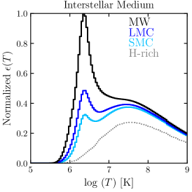
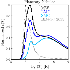
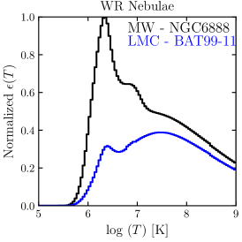
Figure 1: Emission coefficient $\epsilon(T)$ for the 0.3–2.0 keV energy range computed for different abundance sets. Left: ISM abundances from the Milky Way (MW) and the Large and Small Magellanic Clouds (LMC and SMC). For comparison we also show the result for a pure hydrogen gas. Center: PNe abundances. Right: Computed for two iconic WR nebulae abundances. The central panel also shows the results for the hydrogen-poor PN BD$+$30^∘3639 abundance set, which has been divided by 10 to fit on the same scale. The emission coefficient in each panel has been scaled to the corresponding MW value.

We begin by defining the two main tools we use in our analysis: the emission coefficient and the differential emission measure.

2.1 Emission coefficient

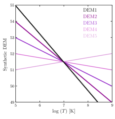
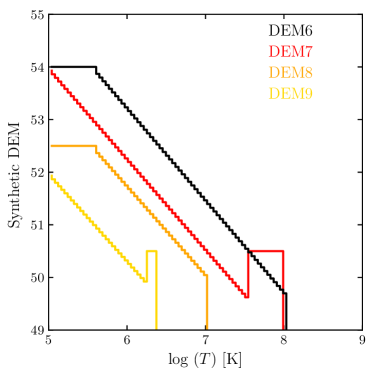
Figure 2: Representative synthetic differential emission measure (DEM) profiles. Left panel: generic DEM profiles with different slopes. Right panel: profiles typical of wind bubbles with evolving central stars.

The emissivity $\epsilon(T,E)$ takes into account the sum of all the contributions to the emission spectrum (e.g., collisionally excited lines, free-free, free-bound and two-photon continua, etc.) made by diffuse gas at a single temperature $T$. It also depends on the chemical abundances. The individual spectra for 100 temperature bins at 0.04 dex intervals in the range $5\leq\log(T)\leq 9$ were calculated using the chianti atomic database. The spectra all have bin widths of 0.01 Å  and a spectral-line full width at half maximum of 0.1 Å  is assumed. The emission coefficient over the X-ray energy band $[E_{1},E_{2}]$ is then defined as

$$\epsilon(T)=\int^{E_{\mathrm{2}}}_{E_{\mathrm{1}}}{\epsilon(T,E)dE}\ \ .$$ (2)

For the X-ray telescopes Chandra and XMM-Newton, the soft energy band corresponds to $E_{\mathrm{1}}=0.3$ keV and $E_{\mathrm{2}}=2.0$ keV.

In Figure 1 we plot the emission coefficient calculated for the following different abundance sets (see Appendix A for actual values):

1. Interstellar medium (ISM) abundances in the Milky Way (MW), the Large Magellanic Cloud (LMC) and the Small Magellanic Cloud (SMC).

2. Planetary nebulae (PN) abundances in the MW, LMC and SMC. Also, the hydrogen-poor PN BD$+30^{\circ}3639$, which is the brightest PN in X-rays in our Galaxy.

3. The representative WR nebulae NGC 6888, which is the most studied WR nebula in the MW, and BAT99-11 in the LMC.

4. Pure hydrogen gas.

For all the abundance sets except the pure hydrogen case, the emission coefficient has two characteristic features: a narrow peak at 1–$3\times 10^{6}$ K and a broad plateau or bump at higher temperatures. The exact position of the narrow peak, and the relative heights of the peak and broad bump change with metallicity. For Milky Way ISM abundances the narrow peak is twice the height of the broad bump, while for SMC ISM abundances the broad bump is marginally higher than the narrow peak. The pure hydrogen case has only the broad, high-temperature feature, thus the narrow peak can be associated directly to line emission from metals.

2.2 Differential Emission Measure

A useful tool for summarizing the hot gas properties of a numerical simulation, under the assumption that the hot bubble is optically thin at X-ray wavelengths, is the Differential Emission Measure (DEM), which we define as

$$\mathrm{DEM}(T_{\mathrm{b}})=\sum_{k,T_{k}\in T_{\mathrm{b}}}n_{\mathrm{e}}^{2}\Delta V_{k},$$ (3)

where $n_{\mathrm{e}}$ is the electron number density in cell $k$, $\Delta V_{k}$ is the volume of cell $k$ and the sum is performed over cells with gas temperature falling in the bin whose central temperature is $T_{\mathrm{b}}$ (see also Strickland & Stevens, 1998).

The DEM profile will be different for different types of astrophysical object and, for a given object, will evolve with time. For example, a PN has a stellar wind whose terminal velocity increases rapidly over a short timescale. This means that the temperature behind the inner wind shock will increase with time.

In Figure 2 we show synthetic DEMs, which cover a range of hypothetical behaviours. The left panel, showing DEM1–5, presents arbitrary DEMs that illustrate a variety of different slopes corresponding to power-law indices from $-1.75$ to $+0.25$. The right panel, showing DEM6–9, presents DEMs that are characteristic of stellar wind bubbles, WR nebulae and PNe such as those we have modeled using numerial simulations in previous work (see Toalá & Arthur, 2011, and Paper I). The temperature spread of these profiles reflects both the evolution of the stellar wind velocity and the effect of mixing seen at the edge of the hot bubble in our 2D simulations. The profiles with flat regions at $T<10^{6}$ K mimic the behaviour of models with thermal conduction, where the lower temperature region corresponds to the conduction layer. Note that a uniform velocity stellar wind with no mixing (e.g., Arthur, 2012) would give a DEM profile consisting of a single spike in the temperature bin corresponding to the postshock temperature.

2.3 Mean temperature

X-ray observations of hot bubbles often report a single plasma temperature ($T_{\mathrm{X}}$). This plasma temperature is obtained by fitting a single-component optically-thin plasma emission model to the observed spectrum (apec or mekal model).

We can use the emission coefficient and the DEM distribution to calculate an average temperature for the hot bubbles generated by numerical simulations. This temperature will be closer to the observationally derived X-ray temperature than either a mass-weighted or volume-weighted mean temperature (see, e.g., Rogers & Pittard, 2014). Strickland & Stevens (1998) defined an intrinsic (i.e., unabsorbed) flux-weighted average temperature $\langle T_{\mathrm{EW}}\rangle$ over the whole 0.005–15 keV energy range. Their definition results in very low average temperatures because it gives too much weight to cool gas emitting mainly in the UV.

In Paper I we defined the mean temperature as

$$T_{\mathrm{A}}=\frac{\int{\epsilon(T)\mathrm{DEM}(T)TdT}}{\int{\epsilon(T)\mathrm{DEM}(T)dT}},$$ (4)

where $\epsilon(T)$ is the emission coefficient in the X-ray band and $\mathrm{DEM}(T)$ is the differential emission measure at temperature $T$. The integral is performed over all the temperature bins of the simulation. This mean temperature is weighted by both emission coefficent and DEM and so takes into account the chemical abundances together with the mass and volume distribution of the hot gas. Although the $\mathrm{DEM}(T)$ profile itself may be weighted towards low temperatures ($T\sim 10^{5}$ K), the fact that the emission coefficient $\epsilon(T)$ is sharply peaked around a few times $10^{6}$ K means that gas with this temperature is preferentially selected (see figure 5 in Paper I), i.e., the emission coefficient acts as a temperature filter.

Table 1: Average temperatures ($T_{\mathrm{A}}$) in logarithmic values calculated for different DEMs and abundance sets.

Abundance	DEM1	DEM2	DEM3	DEM4	DEM5	DEM6	DEM7	DEM8	DEM9	DEMf
set
ISM-MW	6.306	6.502	6.928	7.614	8.237	6.300	6.482	6.268	6.218	7.957
ISM-LMC	6.384	6.630	7.107	7.757	8.293	6.374	6.644	6.314	6.230	8.055
ISM-SMC	6.459	6.739	7.216	7.826	8.315	6.446	6.774	6.362	6.243	8.098
PN-MW	6.200	6.379	6.802	7.529	8.210	6.197	6.335	6.176	6.168	7.903
PN-LMC	6.262	6.481	6.955	7.662	8.264	6.255	6.457	6.218	6.189	7.998
PN-SMC	6.461	6.742	7.230	7.837	8.319	6.448	6.784	6.360	6.242	8.105
BD$+30^{\circ}$3639	6.060	6.127	6.263	6.696	7.573	6.060	6.076	6.062	6.100	7.102
WR-MW (NGC 6888)	6.281	6.478	6.905	7.593	8.226	6.276	6.448	6.245	6.202	7.940
WR-LMC (BAT99-11)	6.400	6.685	7.186	7.814	8.312	6.388	6.703	6.310	6.216	8.092

2.4 Test Results

Table 1 reports the average temperatures obtained from combining the emission coefficients of Figure 1 with the DEM distributions of Figure 2 using Equation 4. Also included is the mean temperature that would be obtained from a completely flat DEM distribution (column DEM_f). There are two clear trends. Firstly, the mean temperature increases as the DEM slope (as a function of bin temperature) goes from steeply negative to positive. Secondly, the mean temperature increases with decreasing metallicity. Thus, for example, objects with a similar history (same DEM) will appear to be hotter in the SMC than in the Milky Way. Also, average temperatures for objects with enhanced abundances such as PNe and WR nebulae will be lower than objects such as stellar wind bubbles with ISM abundances, even though the DEM profiles are similar.

3 Results

We apply our methods to the results of 2D axisymmetric numerical simulations of PNe, WR nebulae and stellar wind bubbles in HII regions. These simulations have been reported in Toalá & Arthur (2014), Paper I, Toalá & Arthur (2011) and Arthur & Hoare (2006), respectively. Full details of the numerical codes used can be found in the cited references. In particular, in simulations with thermal conduction, the conduction is isotropic and saturation is taken into account by limiting the electron mean free path (Toalá & Arthur, 2014).

3.1 Simulated PNe

Figure 3: DEM profiles from selected times in the evolution of a PNe around a central star whose initial ZAMS mass was $1.5M_{\odot}$ and whose final white dwarf mass will be $0.597M_{\odot}$ (see Paper I).

For PNe, the timescales are so short (less than 10,000 yr) that radiative cooling is not yet important for the hot, shocked fast wind gas. The DEM profiles for a set of simulations corresponding to a $1.5M_{\odot}$ progenitor star that ends its life as a $0.597M_{\odot}$ white dwarf are shown in Figure 3. The upper panel is for simulations without thermal conduction, while the lower panel is for simulations where thermal conduction was included. Both sets of results show that the DEM profiles become steeper with time and that the maximum temperature of the profile moves to higher values. This is because the stellar wind velocity of the central star increases with time and the maximum temperature reflects the immediate postshock temperature at the inner wind shock.

The continuous spread of the DEM profile with temperature is typical of wind bubbles with turbulent mixing layers. Instabilities in the swept-up shell lead to the formation of filaments and clumps that interact with the fast wind and the ionizing photons resulting in gas with intermediate densities and temperatures between the hot, shocked fast wind and the warm, photoionized dense shell. The nebular gas is heated by shocks formed in hydrodynamic interactions in material photoevaporated or ablated from the filaments and clumps. Pressure fluctuations in the shocked fast wind as it squeezes past the obstacles lead to temperature fluctuations in the hot plasma. These hydrodynamic effects are not seen in 1D simulations (see Paper I).

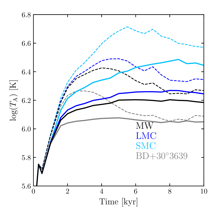
Figure 4: Evolution of the emission-coefficient-weighted mean temperature of simulated PNe for a $1.5M_{\odot}$ progenitor star for different abundance sets. The solid lines correspond to simulations with thermal conduction, the dashed lines are for simulations without conduction.

When conduction is included in the calculations, thermal energy is efficiently transferred from the hottest gas to the dense shell where it evaporates material into the conduction layer. This smoothes out the DEM profile at higher temperatures and the conduction layer results in the characteristic plateau for $\log_{\mathrm{10}}T<5.7$. The main body of the DEM profile has a very similar slope to the models without conduction but the DEM values are higher for a given temperature.

The emission-coefficient-weighted mean temperature as a function of time for these simulations is plotted in Figure 4 for PNe abundances in the Galaxy, the LMC and the SMC, and can be understood in the context of the test cases described in Section 2.4. The slopes of the DEM profiles for the models without conduction steepen with time and so we would expect the average temperature at early times to be higher but then tend to the peak value of the corresponding emission coefficient at later times. For the models with conduction, the plateau at $\log_{10}T<5.7$ K and smooth slope all the way to the maximum temperature lead to faster convergence of the mean temperature. The abundance set determines the maximum mean temperature: the Milky Way abundances result in $\log_{10}T_{\mathrm{A}}<6.4$ and a converged value $\log_{10}T_{\mathrm{A}}\sim 6.2$, while the SMC abundances have $\log_{10}T_{\mathrm{A}}<6.7$, which does not converge over the 10,000 yr timescale because of the competition between the DEM profile slope and the relative heights of the narrow and broad peaks of the emission coefficient (see Fig. 1).

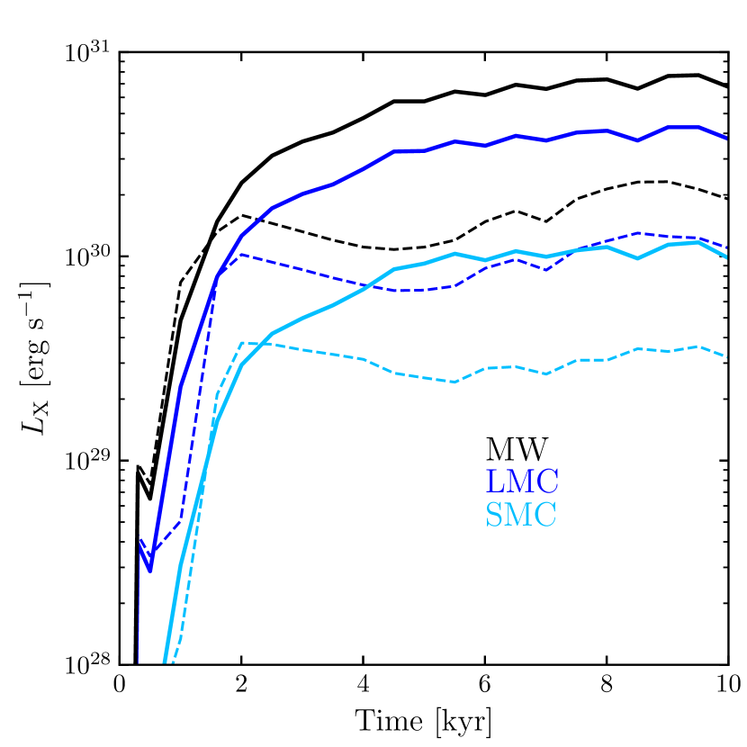
Figure 5: Evolution of the X-ray luminosity of simulated PNe for a $1.5M_{\odot}$ progenitor star for different abundance sets. The solid lines correspond to simulations with thermal conduction, the dashed lines are for simulations without conduction.

Figure 5 shows the luminosities corresponding to the same models as Figure 4. Results for the models with and without thermal conduction are presented. After a short initial evolution, the luminosities remain roughly constant for both types of model. It can be seen that lower metallicity objects are much less luminous, which has consequences for the possible detection of PNe in external, low-metallicity galaxies.

3.2 Simulated Wolf-Rayet Nebulae

WR nebulae are similar to PNe, in the sense that a fast, radiatively driven wind from a hot compact object interacts with a circumstellar medium formed by previous intense mass-loss episodes of the progenitor star. On the other hand, WR nebulae are different to PNe in that the mechanical luminosity of the wind does not drop off with time and the timescale of this evolutionary stage is much longer. Thus, the shocked wind material in the nebula becomes proportionately more significant as time progresses. There will be chemical abundance differences between the hydrogen-rich nebular gas and the fast wind material leaving the hydrogen-poor surface of the star. In particular, all elements such as oxygen, silicon, magnesium and iron should be in the gas phase in the stellar wind material, whereas in the nebular gas they may be partially locked up in silicate dust grains. Higher energy diffuse X-ray emission should reflect the shocked stellar wind, while the lower energy part of the spectrum will be produced by the nebular material.

The evolution of massive stars prior to the WR stage is very varied, depending on progenitor initial mass, metallicity and stellar rotation rate (Ekström et al., 2012; Eldridge & Tout, 2004; Eldridge et al., 2006). The mass expelled during the red supergiant (RSG) or luminous blue variable (LBV) stage can be distributed close to the WR star or in several shells at increasing distances, depending on the details of the mass-loss history (Toalá & Arthur, 2011). Moreover, the velocity of the circumstellar material will below ($\sim 30$ km s^-1) for RSG material but considerably higher ($\sim 200$ km s^-1) for LBV material. These factors affect the details of the wind-wind interaction and the nature of the instabilities that form in the interaction region.

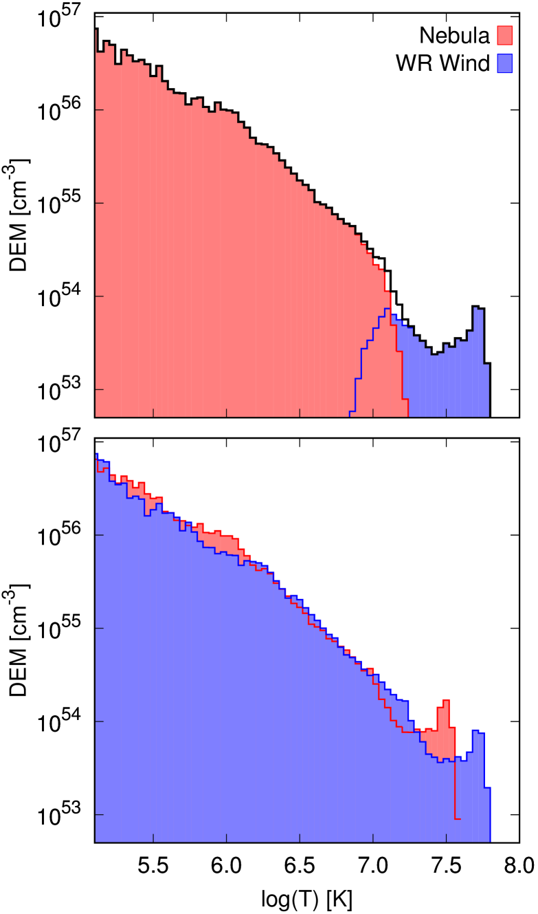
Figure 6: DEM profile for the numerical simulation. Top panel: red histogram is the nebular contribution (scalar $>0.5$) and the blue histogram is the WR fast stellar wind (scalar $<0.5$) contribution. Bottom panel: DEM profiles if the abundances were wholly nebular (red) or wholly WR star (blue) values.

In Appendix B we show the temperature and nebular gas (using an advected scalar label) distributions for a 2D axisymmetric numerical simulation of a simplified WR nebula consisting of a constant velocity fast wind ($v_{\infty}=1600$ km s^-1) interacting with a circumstellar medium generated by a constant slow dense wind that ejected $15M_{\odot}$ of material over a timescale of 200,000 years. Figure 6 shows the DEM profile for this simulation, depicted 15,000 years after the onset of the fast wind. Note that the interaction region produces a full spectrum of gas temperatures, with the nebular gas being heated up to $\log_{10}T\sim 7.2$ by shocks refracted by the clumps and filaments in the swept-up RSG material. On the other hand, the shocked fast-wind temperatures extend down to $\log_{10}T\sim 7.2$ due to pressure and density variations in the complex non-radial flows in the interaction region. The separation in temperature of nebular and wind material is maintained throughout the simulation.

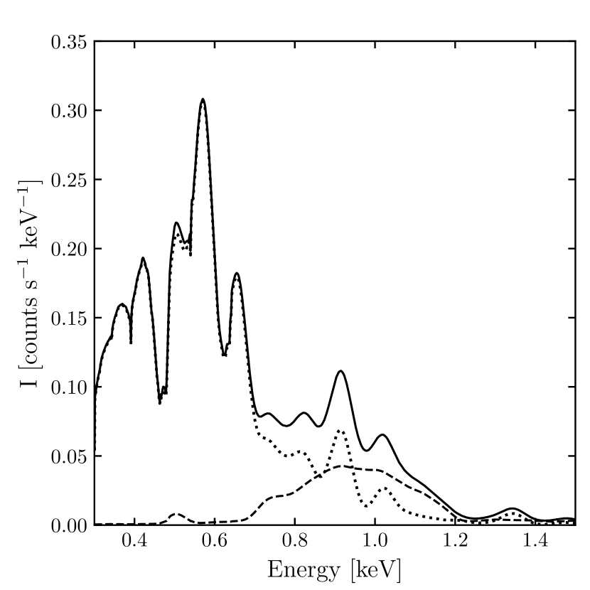
Figure 7: Synthetic spectrum obtained from the DEM profiles shown in Figure 6 (top panel). The spectrum has been corrected for absorption by a neutral hydrogen column density of $N_{\mathrm{H}}=3.13\times$10²¹ cm^-2 and convolved with the instrumental response matrices of the Chandra ACIS-S instrument. The spectrum is binned to a resolution of 60 eV. The solid line represents the total spectrum, the dotted line represents the contribution of the nebular gas and the dashed line shows the contribution of the hot, shocked fast-wind gas

.

The spectrum obtained from the simulation DEM profile (see Fig. 6) assuming abundances as for the galactic WR nebula NGC 6888 (see Table 2) is shown in Figure 7. The intrinsic spectrum has been corrected for the interstellar absorbing neutral hydrogen column density reported for its central star WR 136 ($N_{\mathrm{H}}=3.16\times 10^{21}$ cm^-2; Hamann et al., 1994) and convolved with the instrumental response matrices of Chandra ACIS-S. The total spectrum (solid line) and the contribution of the shocked fast wind (dashed line) indicate that the WR fast wind contributes considerably in the 0.8–1.0 keV spectral energy range. The spectrum shows strong similarities with the observed spectra reported by Toalá et al. (2014) (see also Toalá et al., 2016a, for comparison with XMM-Newton spectra): Most of the emission comes from energies below 0.7 keV with significant emission from the Fe complex and Ne ix line at 0.8–1.2 keV, declining to energies above 1.5 keV. As in other WR nebulae (see, e.g., Toalá et al., 2012), the observed spectrum of NGC 6888 was fit with a two-temperature apec model ($1.4\times 10^{6}$ K and $8.2\times 10^{6}$ K). The second component is necessary to give a good fit for energies above 0.8 keV. In our synthetic spectrum, the hot shocked fast wind continuum emission contributes about half the counts in this range and peaks are lines from an iron complex whose prominance is due to the high iron abundance in the nebular gas, which is closer to solar than to ISM or PNe values in this object.

3.3 Simulated stellar wind bubbles in HII regions

Following the work of Mackey et al. (2015), who studied stellar wind bubbles in HII regions around single O stars moving in a uniform medium, we decided to re-examine the simulations of Arthur & Hoare (2006). The DEM profiles calculated for some of their models are shown in Figure 8. The models that were available correspond to a stellar wind bubble and HII region evolving in (i) a uniform medium with density $n_{0}=6000$ cm^-3, (ii) a plane-stratified medium with exponential density distribution $n=n_{0}\exp(-z/H)$ where the scale height is $H=0.2$ pc and $n_{0}=8000$ cm^-3 (Model E of Arthur & Hoare, 2006) and (iii) a star moving up a density gradient with velocity $V_{*}=10$ km s^-1 (Model H of Arthur & Hoare, 2006). In each model the stellar wind velocity is $v_{\infty}=2000$ km s^-1 and the mass-loss rate is $\dot{M}=10^{-6}M_{\odot}$ yr^-1, while the ionizing photon rate is $2.2\times 10^{48}$ s^-1.

What we see in each case is a steep, negative DEM profile, very similar to the previous results seen for PNe and WR nebulae. Combining these DEM distributions with Milky Way ISM abundances, we find emission-coefficient-weighted mean temperatures of $\log(T_{\mathrm{A}})=6.40$, 6.38 and 6.32 for the uniform medium, exponential medium and moving star models, respectively. This is to be expected, given the form of the DEM profile.

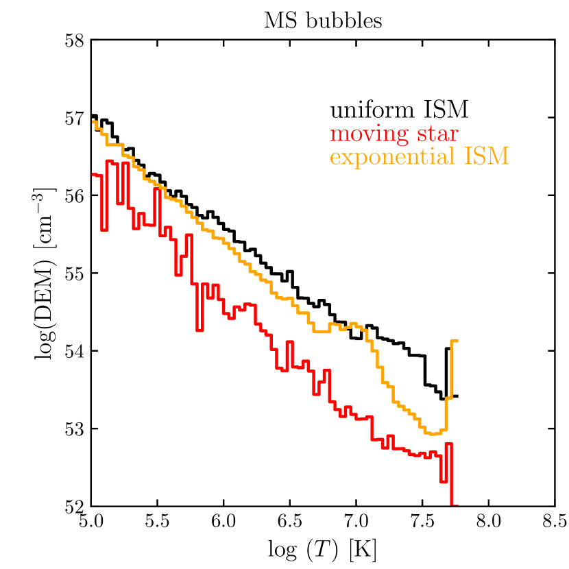
Figure 8: DEM profiles for a stellar wind bubble in an HII region in a uniform medium (black line), an exponential density distribution (yellow line) and a star moving up a density gradient (red line). In each case the simulation represents 20,000 yrs of evolution and the stellar wind parameters are identical (see text).

3.4 Temperature from Spectra

In order to evaluate whether the averaged temperature ($T_{\mathrm{A}}$) is a good estimate to what is obtained from observations ($T_{\mathrm{X}}$), that is, that $T_{\mathrm{A}}\approx T_{\mathrm{X}}$, we took one of the synthetic spectra presented in Paper I and used it as input in xspec (v12.9.0; Arnaud, 1996). We used the synthetic spectrum of the model 1.5-0.597 at 8000 yr without thermal conduction convolved by the Chandra telescope matrices presented in figure 17 in Paper I which has log($T_{\mathrm{A}}$)=6.24 ($kT_{A}$=0.151 keV). The spectrum was modelled assuming the same set of abundances for PNe (see column 5 in Table A1) with a fixed absorbing column density $N_{\mathrm{H}}$=8$\times$10²⁰ cm^-2. The best-fit model turned out to have a plasma temperature of $kT$=0.140 keV, a difference of $\sim$8 per cent with its corresponding $T_{\mathrm{A}}$. Thus, we are confident that the averaged plasma temperature obtained with the method described in Section 2.3 is a good estimate of the temperatures obtained from observations. We remark that the single temperature approach is not representative of the spatial distribution of temperatures in the hot bubble.

4 Discussion

There are 3 main aspects to the temperature of soft X-rays in diffuse objects: the chemical abundances, the actual distribution of temperatures in the diffuse object (i.e., the DEM profile) and the quality of the observations. We discuss PNe, WR nebulae, main sequence wind bubbles and cluster environments in the context of these considerations.

4.1 Planetary Nebulae

The shapes of the emission coefficients shown in Figure 1 are a direct result of the set of chemical abundances used in each case. For PNe, the peak is broader than for either the ISM or WR emission coefficients. The chemical abundances of PNe are the result of the various nucleosynthesis processes that modify the stellar surface chemical composition during the previous AGB-TP phase. The exact details depend on both initial stellar mass and metallicity of the gas from which the star formed. Individual nebulae can be carbon-rich (C/O $>1$) or oxygen-rich (C/O $<1$) depending on whether third dredge-up or hot bottom burning is important in the latter stages of AGB evolution (García-Hernández et al., 2016). Nitrogen can also be enhanced. Our generic PN abundances given in the Appendix represent a carbon-rich object with enhanced nitrogen. The major contributors to the emission coefficient around temperatures of $\sim 10^{6}$ K are bound-bound processes (collisionally excited line emission) of these elements.

In Paper I we showed that at early times the shocked fast wind is the main contributor to the X-ray emission but at later times the nebular gas is the dominant contributor, through the turbulent mixing layer or conduction layer. Thus we could expect evolution in the abundances of the X-ray emitting gas, from CSPN abundances through to PN abundances. The central stars of PNe have been broadly classified into hydrogen-rich and hydrogen-poor (Mendez, 1991; Weidmann, Méndez, & Gamen, 2015). However, there is a large variety of spectral classifications given the peculiar surface abundances and the presence of strong stellar winds.

Although the CHANPLANS program has indicated that up to 30% of their sample have been detected in diffuse X-rays (Kastner et al., 2012; Freeman et al., 2014), only three observations have sufficient spectral resolution and count rate to enable identification of spectral lines. Other PNe with diffuse X-ray detections in the CHANPLANS sample have too few counts ($<200$) to make any conclusive statements regarding spectral features (see Paper I).

The best example is BD$+$30^∘3639, which was observed with the Chandra X-ray telescope, resulting in a spectrum of $\sim 4500$ counts dominated by H-like lines of O viii and C vi and He-like lines of Ne ix and O vii (Yu et al., 2009). Spectral fitting suggests that C and Ne are highly enhanced with respect to O, compared to solar, while N and Fe are depleted. These abundances are consistent with those of the central star, which is a carbon-rich [WR]-type object, thus, no significant mixing has taken place. Spectral modelling suggests a range of plasma temperatures between $1.7\times 10^{6}$ K and $2.9\times 10^{6}$ K, which was determined using a two-component apec model. The current fast wind velocity is $700$ km s^-1 and the dynamical age is only 700 yrs (Leuenhagen et al., 1996). This is a very young, X-ray luminous object. Indeed, the emission coefficient curve for these abundances is almost an order of magnitude higher than the standard PN abundance set. We suggest that the success of the two-component model reflects that the emission coefficient curve peaks at $\log T=6.1$, while the DEM for such a young object will resemble the first profile shown in Figure 3, that is, almost flat but with a peak close to the maximum temperature, which is determined by the current fast wind velocity. The range of temperatures is produced principally by the evolution of the fast-wind velocity.

Another well-observed PN in diffuse X-rays is NGC 6543, the Cat’s Eye nebula. The spectrum of $\sim 1950$ counts has a clearly identifiable He-like emission line triplet of O vii but other lines cannot be unambiguously identified (Guerrero et al., 2015). The central star is hydrogen-rich, classified as OfWR(H) (Weidmann, Méndez, & Gamen, 2015). Spectral modelling with a single temperature plasma suggests a temperature of $1.7\times 10^{6}$ K for the hot gas and there is no evidence for over-abundances of C and Ne with respect ot O, which are modelled with nebular abundances. The data quality is not good enough to determine whether the nitrogen-to-oxygen ratio resembles that of the stellar wind or the nebular value. The fast-wind velocity of the CSPN is $1400$ km s^-1 (Prinja et al., 2007) and so this object is expected to be older than BD$+$30^∘3639, with a more evolved DEM profile (i.e. a steeper slope) and a greater contribution to the X-ray emission from the nebular gas through hydrodynamic interactions and/or thermal conduction (see Paper I).

A third PN, NGC 7027, has been detected in diffuse X-rays with 245 counts (Kastner, Vrtilek, & Soker, 2001). Spectral modelling indicates a plasma temperature of $3\times 10^{6}$ K, near-solar abundances of O and Ne, and overabundances of He, C, N, Mg and Si. The dynamical age of the nebula is only $\sim 600$ yr (Masson, 1989), which is consistent with the extremely high effective temperature of the central object ($T_{\mathrm{eff}}=118$ kK), which is known to be rapidly evolving (Zijlstra, van Hoof, & Perley, 2008). The central star is difficult to observe because of the low contrast with respect to the nebular emission, and no stellar wind parameters are reported for it in the literature. However, we can speculate that the wind will be similiar to or even less evolved than that of BD$+$30^∘3639. Thus, a flat DEM profile dominated by stellar wind material with a peak around the temperature given by the maximum wind velocity would be consistent with the reported diffuse X-ray temperature.

Other cases that exhibit diffuse X-ray emission are the hydrogen-deficient PNe A 30 and A 78 (Chu & Ho, 1995; Chu et al., 1997; Guerrero et al., 2012; Toalá et al., 2015a). A 30 and A 78 are part of the selected small number of PNe classified as born-again PNe in which the central star has experienced a very late thermal pulse (e.g., Herwig et al., 1999). These objects represent the coolest among all diffuse X-ray-emitters with plasma temperatures of $T_{\mathrm{X}}\lesssim$10⁶ K. In these cases the carbon-rich fast wind ($v_{\infty}\gtrsim$3000 km s^-1) from the central star slams into the hydrogen-poor material ejected from the very late thermal pulse producing a variety of complex dynamical processes (mass-loading, ablation, hydrodynamical mixing, etc) along with photoevaporation caused by the strong ionizing UV flux from the central star (Fang et al., 2014). These processes mix the metal-rich material creating pockets of X-ray-emitting gas, which will have an emission coefficient similar to that of BD$+$30^∘3639 (see Fig. 1 central panel), enhancing the production of very soft temperatures. Detailed simulations on the formation and X-ray emission from these objects will be desirable in order to deepen our understanding on the production of X-ray-emitting gas in such unique environments (Toalá & Arthur in prep.).

4.2 Wolf-Rayet Nebulae

The abundances for NGC 6888 given in Table 2 come from the most recent deep spectral study of this object by Esteban et al. (2016). There is enhanced He and N in this object, normal C abundance and some evidence of O deficiency, compared to solar. Interestingly, the nebular Fe abundance is closer to solar than to Galactic ISM abundances. This suggests that a substantial fraction of Fe is in the gas phase rather than being locked up in grains. It is this Fe abundance that is responsible for the plateau seen in the emission coefficient curve around log${}_{10}(T)\sim$ 6.7. The stellar surface abundances of WR136, as determined from stellar atmosphere model fits to optical and UV spectra (Reyes-Pérez et al., 2015) show increased He/O, N/O and Fe/O abundances, while C/O is diminished.

Diffuse X-ray emission has been detected in four WR nebulae: S 308, NGC 2359, NGC 3199 and NGC6888 around WR 6, WR 7, WR 18 and WR 136, respectively (Toalá et al., 2012, 2015b, 2016a, 2017). The spectral type of the central star of NGC 6888, WR136, is WN6, while the other three central stars are all WN4. The stellar wind velocities of the central stars are all very similar, between 1600 and 1800 km s^-1. These WR nebulae are much more extended than PNe detected with CHANPLANS, ranging from a radius of 2.5 pc (NGC 2359) to 9 pc (S 308) and a large number of total counts ($\sim 10,000$) is required to restrict the X-ray-emitting gas parameters. A general property of WR nebula X-ray spectra is the presence of two distinct temperature components. In the best-observed objects, NGC 3199 and NGC 6888, the principal component corresponds to gas at about $1.3\times 10^{6}$ K and accounts for around 90% of the flux, while the second corresponds to higher temperature gas of about $8.3\times 10^{6}$ K and represents $<8\%$ of the flux. The other two objects, S 308 and NGC 2359, have higher temperature second components ($>10^{7}$ K) but the derivation is more uncertain.

Our test simulation, reported in Appendix B shows that the two-component temperature distribution is due principally to the abundance set in the nebular gas as long as a fully populated DEM profile is present. The negative slope of the DEM profile means that the higher temperature component will never dominate the emission. The DEM profile (see Fig. 6) spans a full range of temperatures from photoionized gas through to the immediate post-shock temperature of the fast wind material. This is because the complex hydrodynamic interactions around the clumps and filaments formed by instabilities in the wind-wind interaction raise the temperature of the nebular material. Thus, rather than indicating two independent components with different temperatures, the X-ray spectra are telling us something about the gas-phase abundances in these objects. Esteban et al. (2016) report iron abundances an order of magnitude higher than ISM or average PN values for both S308 and NGC 6888. The high iron abundance responsible for the second component could be related to the life-cycle of grains in the RSG and WR stages of evolution. There are two possibilities, (i) that silicate grains never form in the atmosphere of the RSG (or yellow hypergiant) stage prior to the WR stage (ii) that the grains are destroyed by shock waves once the fast wind starts to sweep up the circumstellar medium.

4.3 Bubbles around hot main-sequence stars

It would be reasonable to think that hot main-sequence stars, sources of ionizing photons and possessing fast stellar winds, are prime candidates for diffuse X-ray emission. Indeed, many star-forming regions have been observed with the Chandra X-ray telescope (see, e.g., Townsley et al., 2014, for a full catalogue of observations). However, the data analysis of these observations is notoriously complicated, with background subtraction and point source excision requiring special treatment (Broos et al., 2010; Townsley et al., 2011b). Diffuse X-ray emission has been found associated with every massive star-forming region observed with Chandra and this emission has been attributed to hot plasma from stellar wind shocks (Townsley et al., 2014). When compared to observations at other wavelengths of the same regions, the diffuse X-ray emission in the 0.5–7 keV band is anticorrelated with the Spitzer mid-IR emission tracing the boundaries of the massive star-forming regions. It occupies the cavities in the molecular clouds and also appears to leak out through fissures in the clouds (cf. Rogers & Pittard, 2013).

The massive star-forming regions detected in diffuse X-rays typically contain clusters of massive stars and some of the regions will certainly have had supernova activity, which will contribute to the diffuse emission. The diffuse X-ray emission has been characterized for a handful of objects, with the best determinations made for the Carina Nebula ($\sim 1.0\times 10^{6}$ net counts) and M17 ($1.5\times 10^{5}$ net counts). The spectra were fitted with several components, where the principal component for the Carina Nebula has $kT=0.31$ keV ($3.6\times 10^{6}$ K), while that for M17 has $kT=0.28$ keV ($3.25\times 10^{6}$ K) (Townsley et al., 2011b). Carina is a star-forming complex containing 8 open clusters and of order 70 ionizing sources, including the luminous blue variable $\eta$ Car. The detection of neutron stars in Carina implies that there have been core-collapse supernova events. On the other hand, M17 is a very young giant HII region ($\sim 0.5\times 10^{6}$ yrs) with 14 known O stars. The estimated total band intrinsic luminosity of the Carina Nebula is an order of magnitude higher than that of M17 ($L_{\mathrm{X}}=1.7\times 10^{35}$ erg s^-1 against $L_{\mathrm{X}}=2\times 10^{34}$ erg s^-1 ).

The Orion Nebula is a young (age $<2\times 10^{6}$ yrs) compact HII region with 2 O stars and 7 early B stars. Diffuse X-ray emission from what is known as the Extended Orion Nebula, observed with XMM-Newton and reported by Güdel et al. (2008), is characterized by a temperature $\sim 2\times 10^{6}$ K and an estimated total band intrinsic luminosity 400 times less than that of M17. The diffuse emission is offset from the position of the ionizing stars, being located to the southwest in the low-density region furthest away from the main ionizing front.

Most recently, faint diffuse thermal X-ray emission characterized by a temperature of $2\times 10^{6}$ K has been detected around the runaway O star $\zeta$ Oph (Toalá et al., 2016b) with a total luminosity in the 0.4–4.0 keV energy range of $L_{\mathrm{X}}=7.6\times 10^{29}$ erg s^-1. The diffuse emission comes from the wake region of the bowshock structure around this isolated O9.5 star, which is moving through the interstellar medium at $\sim~{}30$ km s^-1. This is consistent with the results of numerical simulations of stellar wind bubbles around moving O stars by Mackey et al. (2015), who predicted that soft, faint X-ray emission is produced at the wake of the bow shock in the turbulent mixing layer between the hot, shocked stellar wind and the warm, photoionized gas of the HII region. However, currently $\zeta$ Oph is the only isolated O star with associated diffuse thermal X-ray emission.

We suspect that the surprisingly similar derived X-ray temperatures for these disparate objects have a common origin, namely that turbulent dissipation of the hot shocked fast wind energy in a mixing layer at the interface with the photoionized gas of the HII region forms the characteristic negative slope of the DEM profile. The emission coefficient applied to this DEM “selects” the gas with temperature close to the peak and this is representative of the derived X-ray temperature. For typical ISM or HII region abundances this temperature corresponds to $\log T=6.5$, i.e. $T\sim 2\times 10^{6}$ K. The turbulence at the interface can be triggered by many factors (Breitschwerdt & Kahn, 1988; Kahn & Breitschwerdt, 1990; Mackey et al., 2015): for single star bubbles in uniform media, the cooling swept-up shell can become unstable and the shadowing instability can enhance the instability and turbulence is generated as the hot shocked wind flows through gaps in the swept-up shell. Large-scale density gradients exist in many observed HII regions and these lead to shear flows, which generate turbulence (Arthur & Hoare, 2006). Moving stars in uniform media or density gradients also generate shear flows (Mackey et al., 2015; Arthur & Hoare, 2006). On the other hand, massive star-forming regions form in clumpy molecular clouds, where density inhomogeneities quickly lead to non-radial motions even in the photoionized gas (Mellema et al., 2006; Arthur et al., 2011; Medina et al., 2014).

The size of the turbulent mixing layer will depend on to what extent the stellar wind or the HII region dominates the dynamics of the bubble. Different authors have derived criteria for when the stellar wind can trap the ionization front (Raga et al., 2012; Capriotti & Kozminski, 2001; Weaver et al., 1977) but essentially high stellar wind mass-loss rate favours wind dominance and high photoionization rate favours HII region dominance. When the photoionized gas dominates the dynamics, a thick HII region forms outside the hot bubble and the turbulence is suppressed. In general, the stellar wind may dominate at very early times but the HII region can take over at later times. More extensive mixing layers appear to be favoured when the stellar wind is more dominant or when the shear layer becomes well developed in bubbles formed in density gradients (i.e., steep gradients) or around moving stars. The luminosity of the diffuse X-ray emission will be determined by the amount of gas in the turbulent mixing layer but the temperature is determined by the slope of the DEM distribution for temperatures around the peak of the emission coefficient.

4.4 Numerical Effects

Thus far we have not mentioned numerical effects in the hydrodynamic simulations. The hydrodynamical codes providing the results for this paper discretize the conservation form of the Euler equations and use a piecewise linear approximation to the fluid variables to construct the fluxes at the interfaces between computational cells by solving the Riemann problems here (Godunov, 1959; van Leer, 1977). The codes are second order in time and space (see Arthur & Hoare, 2006; Toalá & Arthur, 2011 for details of the codes). The numerical approximations have an associated truncation error, which leads to numerical diffusion (i.e., smearing) of features in the flow. The effects of numerical diffusion are most obvious at contact discontinuities between two fluids of different densities but equal pressures, where diffusion reduces the sharpness of the contact discontinuity. Furthermore, averaging of fluid properties within grid cells blurs local, i.e., small-scale discontinuities. Increasing the spatial resolution of the simulation can ameliorate the effects of numerical diffusion to a large extent, at the expense of computational memory and calculation time requirements. The effects of numerical diffusion on the outcomes of Eulerian hydrodynamical simulations of advected contact discontinuities and the growth and development of Kelvin-Helmholtz instabilities were discussed in depth by Robertson et al. (2010).

An associated problem has been termed numerical conduction by Parkin & Pittard (2010). At a contact discontinuity, the pressure is continuous but the density is discontinuous and so there should be a sharp discontinuity in the temperature on either side of the interface. Any smearing of the density distribution leads to a corresponding smearing of the temperature distribution. This can result in anomalous cooling in these intermediate-temperature grid cells or even order-of-magnitude overestimates of the X-ray luminosity (Parkin & Pittard, 2010).

In the present paper, we have discussed the results of previously published simulations of WR nebulae, PNe and HII regions. In the wind-blown bubble calculations, the interaction of the fast stellar wind with the surrounding circumstellar medium triggers instabilities in the thin, dense swept-up shell, which are exacerbated by the shadowing instability caused by photoionization and result in the break-up of the shell into clumps (Toalá & Arthur, 2011; Toalá et al., 2014; Arthur, 2015, Paper I). The clumps travel outwards more slowly than the main shock wave and the flow of the shocked fast wind around the clumps generates shear flows, which ablate the clump material and form the turbulent mixing layers. In the case of the HII region simulations (Arthur & Hoare, 2006), Kelvin-Helmholtz instabilities are generated near the head of the champagne-flow or bow-shock models and propagate along the interface between the shocked stellar wind and the photoionized medium, which leads to turbulent mixing layers downstream. In all of these simulations, numerical resolution plays a rôle in determining some of the properties of the clumps resulting from the instabilities, for example, their size and density (Arthur & Hoare, 2006). The size of the wind injection region can influence the number of clumps formed (Toalá & Arthur, 2014). On the other hand, short wavelength instabilities in the shear flows are damped in our simulations because the photoionization softens the density distribution around the dense clumps through photoevaporation, while the timescales of the simulations are too short for radiative cooling to be important in any component of the gas.

If we compare the simulations with and without thermal conduction, for example the PNe simulations reported in Toalá & Arthur (2014) and Paper I, we can assess how extreme diffusion affects the results: it increases the X-ray luminosity in the Chandra soft band by an order of magnitude. We can infer from this that numerical diffusion will affect the X-ray luminosity of the simulated objects. However, the main result of the present paper is unchanged, that is, the X-ray temperature of the hot, diffuse gas is in the observed narrow range [1–3]$\times 10^{6}$ K as a direct consequence of the sharply peaked emission coefficient.

In future work we intend to examine the effects of numerical resolution and diffusion on the properties of X-ray-emitting turbulent mixing layers in the context of the diffuse nebulae discussed in this paper. It is also important to understand how the results of 3-dimensional simulations might differ from the 2-dimensional simulations reported to date (see, e.g., van Marle et al., 2011).

5 SUMMARY

In this paper, we have analyzed the plasma temperature of the hot gas resulting from numerical simulations of diffuse nebulae around main-sequence and evolved stars and we have compared our findings with observations of diffuse X-rays in PNe, WR nebulae, massive star-forming regions and wind-blown bubbles around main-sequence stars. Our method first constructs the differential emission measure (DEM) profile of the simulation and then combines this with the X-ray emission coefficent $\epsilon(T)$ calculated using the atomic database chianti. We have studied the effect of varying the chemical abundances on the emission-coefficient-weighted mean temperature and on the diffuse X-ray spectrum in the Chandra soft energy band. Our main conclusions are:

• Different abundance sets produce their own signature in the X-ray emission coefficient $\epsilon(T)$ in the 0.3–2.0 keV energy range. For all the abundance sets used in this work, except for a pure hydrogen case, $\epsilon(T)$ presents two features: a narrow peak around [1–3]$\times 10^{6}$ K and a broad bump at higher temperatures peaking at $\log_{10}(T)\sim 7.5$. The relative contribution of the narrow peak decreases with decreasing metallicity, such that the pure hydrogen case does not possess a narrow peak. The absolute value of $\epsilon(T)$ is directly related to the X-ray luminosity and increases with increasing metallicity.

• The emission coefficient acts as a filter for the differential emission measure (DEM) profile of the gas and emphasizes the contribution of gas with temperatures close to that of the peak of $\epsilon(T)$ even though the actual temperature distribution of the source is much more complex. For low metallicity gas, the peak of the emission coefficient occurs at slightly higher temperatures.

• The DEM profiles calculated from numerical simulations of PNe, WR nebulae and stellar wind bubbles in H ii regions around main-sequence stars are all remarkably similar and have steep negative slopes over the temperature range $5<\log_{10}(T)<8$. The emission-coefficient-weighted mean temperature of these objects is thus always close to the temperature of the peak of the emission coefficent in the X-ray band. We showed that the averaged plasma temperature is a good estimate to the X-ray-emitting temperature obtained from spectral fits, that is, $T_{\mathrm{A}}\approx T_{\mathrm{X}}$. This is the reason why the temperature derived from observations always turns out to be in the range [1–3]$\times 10^{6}$ K.

• The DEM profiles of the simulated diffuse nebulae are all so similar because in each case turbulent mixing layers transfer energy from the hot shocked stellar wind to the warm ($T\sim 10^{4}$ K) photoionized gas, where it is dissipated. It does not matter whether thermal conduction is included in the simulations or not. Turbulent mixing layers are only produced in 2D or 3D simulations of diffuse nebulae and should be studied in more detail.

• The second temperature component obtained from spectral analysis of the diffuse X-ray emission from WR nebulae is due in part to the shocked fast wind material from the central star. Fast stellar winds from WR stars have much higher mass-loss rates than for either main-sequence stars or the central stars of PNe. A second temperature component has not been reported for these other sorts of objects. In WR nebulae, the wind contributes significantly to the spectrum in the $\sim$0.8–1.2 keV range.

• A diffuse nebula in the SMC will appear to be slightly hotter and up to an order of magnitude less luminous in X-rays than the same object in the Milky Way, simply on the basis of the emission coefficient in the soft X-ray band (0.3–2.0 keV).

Finally, we would like to remark that the number of PNe and WR nebulae that exhibit diffuse X-ray emission is realatively small (4 WR nebulae and only $\sim$30% of all PNe observed in the CHANPLANS survey) and in some cases the spectral quality is not good enough to make a confident analysis of the spectral properties of the X-ray-emitting plasma. It would be interesting to use the future generation of X-ray satellites (e.g., $Athena+$; Nandra et al., 2013) to try to unveil the presence of hotter components in the diffuse emission and properly characterise the abundances of the hot gas in these objects through resolved line emission.

Appendix A Abundance sets

Here we present the details of the abundances used for our calculations.

Table 2: Abundance sets.

Element	ISM			PNe				WR nebulae
	MWa	LMCb	SMCc	MWa	LMCd	SMCe	BD$+$30∘3639f	NGC 6888g	BAT99-11h
He	10.99	10.95	10.91	11.00	11.10	10.99	10.99	11.20	11.01
C	8.40	7.90	7.40	8.89	8.52	7.41	10.59	8.50	7.90
N	7.90	6.90	6.50	8.26	8.24	7.35	7.90	8.53	6.56
O	8.50	8.40	8.00	8.64	8.42	7.89	9.53	8.49	8.23
Ne	8.09	7.39	7.39	8.04	7.60	7.14	8.09	7.81	6.83
Na	5.50	5.50	5.50	6.28	5.50	5.50	6.28	5.50	5.50
Mg	7.10	6.80	6.40	6.20	6.15	6.40	6.20	7.10	6.80
Al	4.90	4.60	4.20	5.43	4.60	4.20	5.43	4.90	4.60
Si	6.50	6.70	6.30	7.00	7.10	6.30	7.00	6.50	6.70
S	7.51	6.77	6.77	7.00	6.94	6.98	7.00	7.23	6.20
Fe	5.80	5.49	5.10	5.70	5.49	5.10	5.70	6.84	5.49

• ^aPredefined for Cloudy (Ferland et al., 2013), ^bSchenck et al. (2016), Hughes et al. (1998) and Korn et al. (2000), ^cKorn et al. (2000), ^dDopita et al. (1997), ^eIdiart et al. (2007), ^fMarcolino et al. (2007) and Yu et al. (2009), ^gEsteban et al. (2016), and ^hStock et al. (2011).

Appendix B Simulation of a Wolf-Rayet Nebula

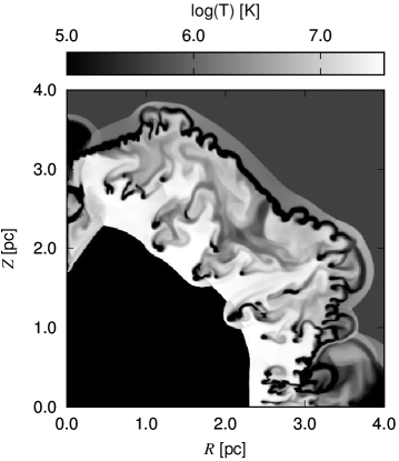
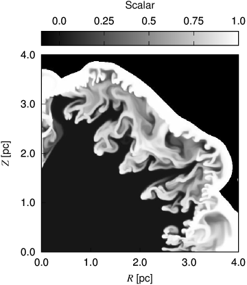
Figure 9: Simulation of a generic WR nebula (see Arthur, 2015). Left panel: gas temperature above $10^{5}$ K. The corrugated swept-up RSG wind shell (black) and the hot, shocked main-sequence bubble material outside it can be clearly distinguished. Right panel: advected scalar, which is used to trace the different components of the nebula. In this panel, negative values correspond to unperturbed main-sequence bubble material, scalar value 0 corresponds to unmixed fast stellar wind, while nebular gas (shocked main-sequence bubble material and RSG wind) has scalar value 1. Intermediate values of the scalar indicate mixing regions between the fast wind and the nebular material.

We have performed 2D axisymmetric simulations of the interaction between a fast wind and a dense circumstellar medium with parameters appropriate to a WR nebula, though without being tailored for any object in particular (Arthur, 2015). The simulations were done on a $500^{2}$ grid using the same code as used for the planetary nebula simulations of Toalá & Arthur (2014) and include photoionization and radiative cooling but thermal conduction is turned off. The chemical abundance set used in this model is appropriate to NGC 6888, the nebula around the WR star WR136. These simulations assume that the initial circumstellar medium represents the expelled RSG envelope and is composed of $15M_{\odot}$ of material that was ejected at a steady rate over 200,000 years at 15 km s^-1 into a uniform, hot ($T=4.27\times 10^{5}$ K), low-density ($n=0.01$ cm^-3), ionized medium (which represents the main-sequence hot, shocked stellar wind bubble). The WR star stellar wind is taken to have a constant velocity $v_{\infty}=1600$ km s^-1 and mass-loss rate $\dot{M}=7\times 10^{-5}M_{\odot}$ yr^-1. The dense shell marking the rim of the RSG wind is initially 2.7 pc from the star.

At the time shown in Figure 9, 15,000 years after the onset of the fast wind, the RSG material has been completely swept up and the bubble has broken out into the low density medium beyond. This is evident in the distribution of the scalar value and the gas temperature shown in the figure. The wind-wind interaction forms an unstable dense shell, which breaks up into knots and filaments as it travels down the $r^{-2}$ density gradient. Complex hydrodynamic interactions as shock waves are refracted around the clumps lead to a full range of gas temperatures in the wind bubble, as can be seen from the DEM profile (Fig. 6). Fast wind material occupies the higher temperature range, $\log T>7.2$, while nebular material dominates temperatures in the range $\log T<7.2$. The unshocked main-sequence-bubble material has a negligible ($<1\%$) contribution to the DEM in the temperature bin at $\log T=5.63$ because the density is so low in this gas.

References

- Arnaud (1996) Arnaud, K. A. 1996, Astronomical Data Analysis Software and Systems V, 101, 17
- Arthur (2012) Arthur, S. J. 2012, MNRAS, 421, 1283
- Arthur (2015) Arthur, S. J. 2015, in W.-R. Hamann, A. Sander, H. Todt ed., Wolf-Rayet Stars, Universitätsverlag Potsdam, p.315
- Arthur et al. (2011) Arthur, S. J., Henney, W. J., Mellema, G., de Colle, F., & Vázquez-Semadeni, E. 2011, MNRAS, 414, 1747
- Arthur & Hoare (2006) Arthur, S. J., & Hoare, M. G. 2006, ApJS, 165, 283
- Breitschwerdt & Kahn (1988) Breitschwerdt, D., & Kahn, F. D. 1988, MNRAS, 235, 1011
- Broos et al. (2010) Broos, P. S., Townsley, L. K., Feigelson, E. D., et al. 2010, ApJ, 714, 1582
- Capriotti & Kozminski (2001) Capriotti, E. R., & Kozminski, J. F. 2001, PASP, 113, 677
- Chu et al. (1997) Chu, Y.-H., Chang, T. H., & Conway, G. M. 1997, ApJ, 482, 891
- Chu & Ho (1995) Chu, Y.-H., & Ho, C.-H. 1995, ApJ, 448, L127
- Dere et al. (2009) Dere, K. P., Landi, E., Young, P. R., et al. 2009, A&A, 498, 915
- Dere et al. (1997) Dere, K. P., Landi, E., Mason, H. E., Monsignori Fossi, B. C., & Young, P. R. 1997, A&AS, 125
- Dopita et al. (1997) Dopita, M. A., Vassiliadis, E., Wood, P. R., et al. 1997, ApJ, 474, 188
- Dyson & Williams (1997) Dyson, J. E., & Williams, D. A. 1997, The physics of the interstellar medium. Edition: 2nd ed. Publisher: Bristol: Institute of Physics Publishing, 1997. Edited by J. E. Dyson and D. A. Williams. Series: The graduate series in astronomy. ISBN: 0750303069
- Ekström et al. (2012) Ekström, S., Georgy, C., Eggenberger, P., et al. 2012, A&A, 537, A146
- Eldridge et al. (2006) Eldridge, J. J., Genet, F., Daigne, F., & Mochkovitch, R. 2006, MNRAS, 367, 186
- Eldridge & Tout (2004) Eldridge, J. J., & Tout, C. A. 2004, MNRAS, 353, 87
- Esteban et al. (2016) Esteban, C., Mesa-Delgado, A., Morisset, C., & García-Rojas, J. 2016, MNRAS, 460, 4038
- Fang et al. (2014) Fang, X., Guerrero, M. A., Marquez-Lugo, R. A., et al. 2014, ApJ, 797, 100
- Ferland et al. (2013) Ferland, G. J., Porter, R. L., van Hoof, P. A. M., et al. 2013, Rev. Mex. Astron. Astrofis., 49, 137
- Freeman et al. (2014) Freeman, M., Montez, R., Jr., Kastner, J. H., et al. 2014, ApJ, 794, 99
- García-Hernández et al. (2016) García-Hernández D. A., Ventura P., Delgado-Inglada G., Dell’Agli F., Di Criscienzo M., Yagüe A., 2016, MNRAS, 461, 542
- Godunov (1959) Godunov, S., 1959, Math. Sbornik, 47, 271
- Güdel et al. (2008) Güdel, M., Briggs, K. R., Montmerle, T., et al. 2008, Science, 319, 309
- Guerrero & De Marco (2013) Guerrero, M. A., & De Marco, O. 2013, A&A, 553, A126
- Guerrero et al. (2012) Guerrero, M. A., Ruiz, N., Hamann, W.-R., et al. 2012, ApJ, 755, 129
- Guerrero et al. (2015) Guerrero M. A., Toalá J. A., Chu Y.-H., Gruendl R. A., 2015, A&A, 574, A1
- Hainich et al. (2015) Hainich, R., Pasemann, D., Todt, H., et al. 2015, A&A, 581, A21
- Hamann et al. (2006) Hamann, W.-R., Gräfener, G., & Liermann, A. 2006, A&A, 457, 1015
- Hamann et al. (1994) Hamann, W.-R., Wessolowski, U., & Koesterke, L. 1994, A&A, 281, 184
- Herwig et al. (1999) Herwig, F., Blöcker, T., Langer, N., & Driebe, T. 1999, A&A, 349, L5
- Hughes et al. (1998) Hughes, J. P., Hayashi, I., & Koyama, K. 1998, ApJ, 505, 732
- Idiart et al. (2007) Idiart, T. P., Maciel, W. J., & Costa, R. D. D. 2007, A&A, 472, 101
- Kahn & Breitschwerdt (1990) Kahn, F. D., & Breitschwerdt, D. 1990, MNRAS, 242, 209
- Kastner, Vrtilek, & Soker (2001) Kastner J. H., Vrtilek S. D., Soker N., 2001, ApJ, 550, L189
- Kastner et al. (2012) Kastner, J. H., Montez, R., Jr., Balick, B., et al. 2012, AJ, 144, 58
- Korn et al. (2000) Korn, A. J., Becker, S. R., Gummersbach, C. A., & Wolf, B. 2000, A&A, 353, 655
- Kwok et al. (1978) Kwok, S., Purton, C. R., & Fitzgerald, P. M. 1978, ApJ, 219, L125
- Landi et al. (2013) Landi, E., Young, P. R., Dere, K. P., Del Zanna, G., & Mason, H. E. 2013, ApJ, 763, 86
- Leuenhagen et al. (1996) Leuenhagen, U., Hamann, W. R., & Jeffery, C. S. 1996, A&A, 312, 167
- Mackey et al. (2015) Mackey, J., Gvaramadze, V. V., Mohamed, S., & Langer, N. 2015, A&A, 573, A10
- Marcolino et al. (2007) Marcolino, W. L. F., Hillier, D. J., de Araujo, F. X., & Pereira, C. B. 2007, ApJ, 654, 1068
- Masson (1989) Masson C. R., 1989, ApJ, 336, 294
- Medina et al. (2014) Medina, S.-N. X., Arthur, S. J., Henney, W. J., Mellema, G., & Gazol, A. 2014, MNRAS, 445, 1797
- Mellema et al. (2006) Mellema, G., Arthur, S. J., Henney, W. J., Iliev, I. T., & Shapiro, P. R. 2006, ApJ, 647, 397
- Mendez (1991) Mendez R. H., 1991, IAUS, 145, 375
- Nandra et al. (2013) Nandra, K., Barret, D., Barcons, X., et al. 2013, arXiv:1306.2307
- Parkin & Pittard (2010) Parkin, E. R., & Pittard, J. M. 2010, MNRAS, 406, 2373
- Prinja et al. (2007) Prinja, R. K., Hodges, S. E., Massa, D. L., Fullerton, A. W., & Burnley, A. W. 2007, MNRAS, 382, 299
- Raga et al. (2012) Raga, A. C., Cantó, J., & Rodríguez, L. F. 2012, Rev. Mex. Astron. Astrofis., 48, 199
- Reyes-Iturbide et al. (2009) Reyes-Iturbide, J., Velázquez, P. F., Rosado, M., et al. 2009, MNRAS, 394, 1009
- Reyes-Pérez et al. (2015) Reyes-Pérez, J., Morisset, C., Peña, M., & Mesa-Delgado, A. 2015, MNRAS, 452, 1764
- Robertson et al. (2010) Robertson, B. E., Kravtsov, A. V., Gnedin, N. Y., Abel, T., & Rudd, D. H. 2010, MNRAS, 401, 2463
- Rogers & Pittard (2014) Rogers, H., & Pittard, J. M. 2014, MNRAS, 441, 964
- Rogers & Pittard (2013) Rogers, H., & Pittard, J. M. 2013, MNRAS, 431, 1337
- Ruiz et al. (2013) Ruiz, N., Chu, Y.-H., Gruendl, R. A., et al. 2013, ApJ, 767, 35
- Schenck et al. (2016) Schenck, A., Park, S., & Post, S. 2016, AJ, 151, 161
- Soker (1994) Soker, N. 1994, AJ, 107, 276
- Steffen et al. (2008) Steffen, M., Schönberner, D., & Warmuth, A. 2008, A&A, 489, 173
- Stock et al. (2011) Stock, D. J., Barlow, M. J., & Wesson, R. 2011, MNRAS, 418, 2532