Alleviating partisan gerrymandering: can math and computers help to eliminate wasted votes?

Abstract

Partisan gerrymandering is a major cause for voter disenfranchisement in United States. However, convincing US courts to adopt specific measures to quantify gerrymandering has been of limited success to date. Recently, McGhee in [23] and Stephanopoulos and McGhee in [29] introduced a new and precise measure of partisan gerrymandering via the so-called ”efficiency gap” that computes the absolutes difference of wasted votes between two political parties in a two-party system. Quite importantly from a legal point of view, this measure was found legally convincing enough in a US appeals court in a case that claims that the legislative map of the state of Wisconsin was gerrymandered; the case is now pending in US Supreme Court (Gill v. Whitford, US Supreme Court docket no $16$-$1161$, decision pending). In this article, we show the following:

1. We provide interesting mathematical and computational complexity properties of the problem of minimizing the efficiency gap measure. To the best of our knowledge, these are the first non-trivial theoretical and algorithmic analyses of this measure of gerrymandering.

2. We provide a simple and fast algorithm that can “un-gerrymander” the district maps for the states of Texas, Virginia, Wisconsin and Pennsylvania by bring their efficiency gaps to acceptable levels from the current unacceptable levels. Our work thus shows that, notwithstanding the general worst-case approximation hardness of the efficiency gap measure as shown by us, finding district maps with acceptable levels of efficiency gaps is a computationally tractable problem from a practical point of view. Based on these empirical results, we also provide some interesting insights into three practical issues related the efficiency gap measure.

We believe that, should the US Supreme Court uphold the decision of lower courts, our research work and software will provide a crucial supporting hand to remove partisan gerrymandering.

1 Introduction and Motivation

Gerrymandering, namely creation of district plans with highly asymmetric electoral outcomes to disenfranchise voters, has continued to be a curse to fairness of electoral systems in USA for a long time in spite of general public disdain for it. Even though the US Supreme Court ruled in $1986$ [11] that gerrymandering is justiciable, they could not agree on an effective way of estimating it. Indeed, a huge impediment to removing gerrymandering lies in formulating an effective and precise measure for it that will be acceptable in courts.

In $2006$, the US Supreme Court opined [21] that a measure of partisan symmetry may be a helpful tool to understand and remedy gerrymandering. Partisan symmetry is a standard for defining partisan gerrymandering that involves the computation of counterfactuals typically under the assumption of uniform swings. To illustrate lack of partisan symmetry consider a two-party voting district and suppose that Party A wins by getting $60\%$ of total votes and $70\%$ of total seats. In such a case, a partisan symmetry standard would hold if Party B would also win $70\%$ of the seats had it won $60\%$ of the votes in a hypothetical election. Two frequent indicators cited for lack of partisan symmetry are cracking, namely dividing supporters of a specific party between two or more districts when they could be a majority in a single district, and packing, namely filling a district with more and more supporters of a specific party as long as this does not make this specific party the winner in that district.

There have been many theoretical and empirical attempts at remedying the lack of partisan symmetry by “quantifying” gerrymandering and devising redistricting methods to optimize such quantifications using well-known notions such as compactness and symmetry [25, 7, 6, 8, 26, 18, 3, 16]. Since it is often simply not possible to go over every possible redistricting map to optimize the gerrymandering measure due to rapid combinatorial explosion, researchers such as [22, 30, 7] have also investigated designing efficient algorithmic approach for this purpose. In particular, a popular gerrymandering measure in the literature is symmetry, which attempts to quantify the discrepancy between the share of votes and the share of seats of a party [26, 18, 3, 16]. In spite of such efforts, their success in convincing courts to adopt one or more of these measures has been unfortunately somewhat limited to date.

Recently, researchers Stephanopoulos and McGhee in two papers [23, 29] have introduced a new gerrymandering measure called the “efficiency gap”. Informally speaking, the efficiency gap measure attempts to minimize the absolute difference of total wasted votes between the parties in a two-party electoral system. This measure is very promising in several aspects. Firstly, it provides a mathematically precise measure of gerrymandering with many desirable properties. Equally importantly, at least from a legal point of view, this measure was found legally convincing in a US appeals court in a case that claims that the legislative map of the state of Wisconsin is gerrymandered; the case is now pending in US Supreme Court [17].

1.1 Informal Overview of Our Contribution and Its Significance

Redistricting based on minimizing the efficiency gap measure however requires one to find a solution to an combinatorial optimization problem. To this effect, the contribution of this article is as follows:

1. As a necessary first step towards investigating the efficiency gap measure, in Section 2 we first formalize the optimization problem that corresponds to minimizing the efficiency gap measure.

2. Subsequently, in Section 3 we study the mathematical properties of the formalized version of the measure. Specifically, Lemma 1 and Corollary 2 show that the efficiency gap measure attains only a finite discrete set of rational values; these properties are of considerable importance in understanding the sensitivity of the measure and in designing efficient algorithms for computing this measure.

3. Next, in Sections 4 and 5 we investigate computational complexity and algorithm design issues of redistricting based on the efficiency gap measure. Although Theorem 4 shows that in theory one can construct artificial pathological examples for which designing efficient algorithms is provably hard, Theorem 10 and Theorem 11 provide justification as to why the result in Theorem 4 is overly pessimistic for real data that do not necessarily correspond to these pathological examples. For example, assuming that the districts are geometrically compact ($y$-convex in our terminology), Theorem 11 shows how to find a district map efficiently in polynomial time that minimizes the efficiency gap.

4. Finally, to show that it is indeed possible in practice to solve the problem of minimization of the efficiency gap, in Section 6 we design a fast randomized algorithm based on the local search paradigm in combinatorial optimization for this problem (cf. Fig. 4). Our resulting software was tested on four electoral data for the $2012$ election of the (federal) house of representatives for the US states of Wisconsin [36, 35], Texas [38, 37], Virginia [33, 34] and Pennsylvania [31, 32]. The results computed by our fast algorithm are truly outstanding: the final efficiency gap was lowered to $3.80\%$, $3.33\%$, $3.61\%$ and $8.64\%$ from $14.76\%$, $4.09\%$, $22.25\%$ and $23.80\%$ for Wisconsin, Texas, Virginia and Pennsylvania, respectively, in a small amount of time. Our empirical results clearly show that it is very much possible to design and implement a very fast algorithm that can “un-gerrymander” (with respect to the efficiency gap measure) the gerrymandered US house districts of four US states.

   Based on these empirical results, we also provide some interesting insights into three practical issues related the efficiency gap measure, namely issues pertaining to seat gain vs. efficiency gap, compactness vs. efficiency gap and the naturalness of original gerrymandered districts.

To the best of our knowledge, our results are first algorithmic analysis and implementation of minimization of the efficiency gap measure. Our results show that it is practically feasible to redraw district maps in a small amount of time to remove gerrymandering based on the efficiency gap measure. Thus, should the Supreme Court uphold the ruling of the lower court, our algorithm and its implementation will be a necessary and valuable asset to remove partisan gerrymandering.

1.2 Beyond scientific curiosity: impact on US judicial system

Beyond its scientific implications on the science of gerrymandering, we expect our algorithmic analysis and results to have a beneficial impact on the US judicial system also. Some justices, whether at the Supreme Court level or in lower courts, seem to have a reluctance to taking mathematics, statistics and computing seriously [28, 12], For example, during the hearing in our previously cite most recent US Supreme Court case on gerrymandering [17], some justices opined that the math was unwieldy, complicated, and newfangled. One justice called it baloney, and Chief Justice John Roberts dismissed the attempts to quantify partisan gerrymandering by saying

“It may be simply my educational background, but I can only describe it as sociological gobbledygook.”

Our theoretical and computational results show that the math, whether complicated or not (depending on one’s background), can in fact yield fast accurate computational methods that can indeed be applied to un-gerrymander the currently gerrymandered maps.

1.3 Some Remarks and Explanations Regarding the Technical Content of This Paper

To avoid any possible misgivings or confusions regarding the technical content of the paper as well as to help the reader towards understanding the remaining content of this article, we believe the following comments and explanations may be relevant. We encourage the reader to read this section and explore the references mentioned therein before proceeding further.

1. We employ a randomized local-search heuristic for combinatorial optimization for our algorithm in Fig. 4. Our algorithmic paradigm is quite different from Markov Chain Monte Carlo simulation, simulated annealing approach, Bayesian methods and related similar other methods (e.g., no temperature parameter, no Gibbs sampling, no calculation of transition probabilities based on Markov chain properties, etc.). Thus, for example, our algorithmic paradigm and analysis for the efficiency gap measure is different and incomparable to that used by researchers for other different measure, such as by Herschlag, Ravier and Mattingly [19], by Fifield et al. [13] or by Cho and Liu [8].

   For a detailed exposition of randomized algorithms the reader is referred to excellent textbooks such as [24, 2] and for a detailed exposition of local-search algorithmic paradigm in combinatorial optimization the reader is referred to the excellent textbook [1].

2. While we do provide several non-trivial theoretical algorithmic results, we do not provide any theoretical analysis of the randomized algorithm in Fig. 4. The justification for this is that, due to Theorem 4 and Lemma 12, no such non-trivial theoretical algorithmic complexity results exist in general assuming P$\neq\mathsf{NP}$ for deterministic local-search algorithms or assuming RP$\neq\mathsf{NP}$ for randomized local-search algorithms. One can attribute this to the usual “difference between theory and practice” doctrine.

   For readers unfamiliar with the complexity-theoretic assumptions P$\neq\mathsf{NP}$ and RP$\neq\mathsf{NP}$, these are core complexity-theoretic assumptions that have been routinely used for decades in the field of algorithmic complexity analysis. For example, starting with the famous Cook’s theorem [9] in $1971$ and Karp’s subsequent paper in $1972$ [20], the P$\neq\mathsf{NP}$ assumption is the central assumption in structural complexity theory and algorithmic complexity analysis. For a detailed technical coverage of the basic structural complexity field, we refer the reader to the excellent textbook [4].

3. In this article we use the data at the county level as opposed to using data at finer (more granular) level such as the “Voting Tabulation District” (VTD) level (VTDs are the smallest units in a state for which the election data are available). The reason for this is as follows. Note that our algorithmic approach already returns an efficiency gap of below $4\%$ for three states (namely, WI, TX and VA), and for PA it cuts down the current efficiency gap by a factor of about $3$ (cf. Table 2). This, together with the observation in [29, pp. 886-888] that the efficiency gap should not be minimized to a very low value to avoid unintended consequences, shows that even just by using county-level data our algorithm can already output almost desirable (if not truly desirable) values of the efficient gap measure and thus, by Occam’s razor principle widely used in computer science, we should not be using more data at finer levels. In fact, using more data at a finer level may lead to what is popularly known as “overfitting” in the context of machine learning and elsewhere [5] that may hide its true performance on yet unexplored maps. In this context, our suggestion to future algorithmic researchers in this direction is to use a minimal amount of data that is truly necessary to generate an acceptable solution.

4. In this article we are not comparing our approaches empirically to those in existing literature such as in [19, 13, 8]. The reason for this is that, to the best of our knowledge, there is currently no other published work that gives a software to optimize the efficiency gap measure. In fact, it would be grossly unfair to other existing approaches if we compare our results with their results. For example, suppose we consider an optimal result using an approach from [8] and find that it gives an efficiency gap of $15\%$ whereas the approach in this article gives an efficiency gap of $5\%$. However, it would be grossly unfair to say that, based on this comparison, our algorithm is better than the one in [8] since the authors in [8] never intended to minimize the efficiency gap. Furthermore, even the two maps cannot be compared directly by geometric methods since no court has so far established a firm and unequivocal ground truth on gerrymandering by having a ruling of the following form:

   [court]: “a district map is gerrymandered if and only if such-and-such conditions are satisfied”

   (the line is crossed out above just to doubly clarify that such a ruling does not exist).

   For certain scientific research problems, algorithmic comparisons are possible because of the existence of ground truths (also called ”gold standards” or “benchmarks”). For example, different algorithmic approaches for reverse engineering causal relationships between components of a biological cellular system can be compared by evaluating how close the methods under investigation are in recovering known gold standard networks using widely agreed upon metrics such as recall rates or precision values [10]. Unfortunately, for gerrymandering this is not the case and, in our opinion, comparison of algorithms for gerrymandering that optimize substantially different objectives should be viewed with a grain of salt.

5. The main research goal of this paper is to minimize the efficiency gap measure exactly as introduced by Stephanopoulos and McGhee in [23, 29]. However, should future researchers like to introduce additional computable constraints or objectives, such as compactness or respect of community boundaries, on top of our efficiency gap minimization algorithm, it is a conceptually easy task to modify our algorithm in Fig. 4 for this purpose. For example, to introduce compactness on top of minimization of the efficiency gap measure, the following two lines in Fig. 4

   if $\mathsf{Effgap}_{\kappa}(\mathcal{P},\mathcal{Q}^{\prime}_{1},\dots,\mathcal{Q}^{\prime}_{\kappa})<\mathsf{Effgap}_{\kappa}(\mathcal{P},\mathcal{Q}_{1},\dots,\mathcal{Q}_{\kappa})$ then

   should be changed to something like (changes are indicated in bold):

   if $\mathsf{Effgap}_{\kappa}(\mathcal{P},\mathcal{Q}^{\prime}_{1},\dots,\mathcal{Q}^{\prime}_{\kappa})<\mathsf{Effgap}_{\kappa}(\mathcal{P},\mathcal{Q}_{1},\dots,\mathcal{Q}_{\kappa})$
                          and each of $\boldsymbol{\mathcal{Q}^{\prime}_{1},\dots,\mathcal{Q}^{\prime}_{\kappa}}$ are compact then

   and appropriate minor changes can be made to other parts of the algorithm for consistency with this modification.

2 Formalization of the Optimization Problem to Minimize the Efficiency Gap Measure

Figure 1: Input polygon $\mathcal{P}$ of size $15$ placed on a grid of size $6\times 4$; the cell $p_{2,1}$ is shown.

Based on [23, 29], we abstract our problem in the following manner. We are given a rectilinear polygon $\mathcal{P}$ without holes. Placing $\mathcal{P}$ on a unit grid of size $m\times n$, we will identify an individual unit square (a “cell”) on the $i^{\mathrm{th}}$ row and $j^{\mathrm{th}}$ column in $\mathcal{P}$ by $p_{i,j}$ for $0\leq i<m$ and $0\leq j<n$ (see Fig. 1). For each cell $p_{i,j}\in\mathcal{P}$, we are given the following three integers:

1. an integer ${\mathrm{Pop}}_{i,j}\geq 0$ (the “total population” inside $p_{i,j}$), and

2. two integers ${\mathrm{PartyA}}_{i,j},{\mathrm{PartyB}}_{i,j}\geq 0$ (the total number of voters for Party A and Party B, respectively) such that ${\mathrm{PartyA}}_{i,j}+{\mathrm{PartyB}}_{i,j}={\mathrm{Pop}}_{i,j}$.

Let $|\mathcal{P}|=\left|\,\left\{p_{i,j}\,:\,p_{i,j}\in\mathcal{P}\right\}\,\right|$ denote the “size” (number of cells) of $\mathcal{P}$. For a rectilinear polygon $\mathcal{Q}$ included in the interior of $\mathcal{P}$ (i.e., a connected subset of the interior of $\mathcal{P}$), we defined the following quantities:

Party affiliations in $\mathcal{Q}$:

${\mathrm{PartyA}}(\mathcal{Q})=\sum_{p_{i,j}\in\mathcal{Q}}{\mathrm{PartyA}}_{i,j}$ and ${\mathrm{PartyB}}(\mathcal{Q})=\sum_{p_{i,j}\in\mathcal{Q}}{\mathrm{PartyB}}_{i,j}$.

Population of $\mathcal{Q}$:

${\mathrm{Pop}}(\mathcal{Q})={\mathrm{PartyA}}(\mathcal{Q})+{\mathrm{PartyB}}(\mathcal{Q})$.

Efficiency gap of $\mathcal{Q}$:

$\mathsf{Effgap}(\mathcal{Q})=$

$$\left\{\begin{array}[]{r l}\Big{(}{\mathrm{PartyA}}(\mathcal{Q})-\frac{1}{2}{\mathrm{Pop}}(\mathcal{Q})\Big{)}-{\mathrm{PartyB}}(\mathcal{Q})=2{\mathrm{PartyA}}(\mathcal{Q})-\frac{3}{2}{\mathrm{Pop}}(\mathcal{Q}),&\mbox{if ${\mathrm{PartyA}}(\mathcal{Q})\geq\frac{1}{2}{\mathrm{Pop}}(\mathcal{Q})$}\\[5.0pt] {\mathrm{PartyA}}(\mathcal{Q})-\Big{(}{\mathrm{PartyB}}(\mathcal{Q})-\frac{1}{2}{\mathrm{Pop}}(\mathcal{Q})\Big{)}=2{\mathrm{PartyA}}(\mathcal{Q})-\frac{1}{2}{\mathrm{Pop}}(\mathcal{Q}),&\mbox{otherwise}\end{array}\right.$$

Note that if ${\mathrm{PartyA}}(\mathcal{Q})={\mathrm{PartyB}}(\mathcal{Q})=\frac{1}{2}{\mathrm{Pop}}(\mathcal{Q})$ then $\mathsf{Effgap}(\mathcal{Q})=-{\mathrm{PartyB}}(\mathcal{Q})$, i.e., in case of a tie, we assume Party A is the winner. Also, note that $\mathsf{Effgap}(\mathcal{Q})=0$ if and only if either ${\mathrm{PartyA}}(\mathcal{Q})={{\mathrm{Pop}}(\mathcal{Q})}/{4}$ or ${\mathrm{PartyB}}(\mathcal{Q})={{\mathrm{Pop}}(\mathcal{Q})}/{4}$.

Our problem can now be defined as follows.

Problem name: $\kappa$-district Minimum Wasted Vote Problem (Min-wvp_κ). Input: a rectilinear polygon $\mathcal{P}$ with ${\mathrm{Pop}}_{i,j},{\mathrm{PartyA}}_{i,j},{\mathrm{PartyB}}_{i,j}$ for every cell $p_{i,j}\in\mathcal{P}$, and a positive integer $1<\kappa\leq|\mathcal{P}|$. Definition: a $\kappa$-equipartition of $\mathcal{P}$ is a partition of the interior of $\mathcal{P}$ into exactly $\kappa$ rectilinear polygons, say $\mathcal{Q}_{1},\dots,\mathcal{Q}_{\kappa}$, such that ${\mathrm{Pop}}(\mathcal{Q}_{1})=\dots={\mathrm{Pop}}(\mathcal{Q}_{\kappa})$. Assumption: $\mathcal{P}$ has at least one $\kappa$-equipartition. Valid solution: Any $\kappa$-equipartition $\mathcal{Q}_{1},\dots,\mathcal{Q}_{\kappa}$ of $\mathcal{P}$. Objective: minimize the total absolute efficiency gap$\mathsf{Effgap}_{\kappa}(\mathcal{P},\mathcal{Q}_{1},\dots,\mathcal{Q}_{\kappa})=\left|\,\sum_{j=1}^{\kappa}\mathsf{Effgap}(\mathcal{Q}_{j})\,\right|$. Notation: ${\mathsf{OPT}}_{\kappa}(\mathcal{P})\stackrel{{\scriptstyle\mathrm{def}}}{{=}}\min\left\{\,\mathsf{Effgap}_{\kappa}(\mathcal{P},\mathcal{Q}_{1},\dots,\mathcal{Q}_{\kappa})\,\,|\text{ $\mathcal{Q}_{1},\dots,\mathcal{Q}_{\kappa}$ is a $\kappa$-equipartition of $\mathcal{P}$}\right\}$.

3 Mathematical Properties of Efficiency Gaps: Set of Values Attainable by the Efficiency Gap Measure

The following lemma sheds some light on the set of rational numbers that the total efficiency gap of a $\kappa$-equipartition can take. As an illustrative example, if we just partition the polygon $\mathcal{P}$ into $\kappa=2$ regions, then $\mathsf{Effgap}_{2}(\mathcal{P},\mathcal{Q}_{1},\mathcal{Q}_{2})$ can only be one of the following $3$ possible values:

$$\left|\,2\,{\mathrm{PartyA}}(\mathcal{P})-\frac{1}{2}\,{\mathrm{Pop}}(\mathcal{P})\,\right|\,\,\text{ or }\,\,\left|\,2\,{\mathrm{PartyA}}(\mathcal{P})-{\mathrm{Pop}}(\mathcal{P})\,\right|\,\,\text{ or }\,\,\left|\,2\,{\mathrm{PartyA}}(\mathcal{P})-\frac{3}{2}\,{\mathrm{Pop}}(\mathcal{P})\,\right|$$

Lemma 1

 

(a)

For any $\kappa$-equipartition $\mathcal{Q}_{1},\dots,\mathcal{Q}_{\kappa}$ of $\mathcal{P}$, $\mathsf{Effgap}_{\kappa}(\mathcal{P},\mathcal{Q}_{1},\dots,\mathcal{Q}_{\kappa})$ always assumes one of the $\kappa+1$ values of the form $\left|\,2\,{\mathrm{PartyA}}(\mathcal{P})-\Big{(}z+\frac{\kappa}{2}\Big{)}\frac{{\mathrm{Pop}}(\mathcal{P})}{\kappa}\,\right|$ for $z=0,1,\dots,\kappa$.

(b)

If $\mathsf{Effgap}_{\kappa}(\mathcal{P},\mathcal{Q}_{1},\dots,\mathcal{Q}_{\kappa})=\left|\,2\,{\mathrm{PartyA}}(\mathcal{P})-\Big{(}z+\frac{\kappa}{2}\Big{)}\frac{{\mathrm{Pop}}(\mathcal{P})}{\kappa}\,\right|$ for some $z\in\{0,1,\dots,\kappa\}$ and some $\kappa$-equipartition $\mathcal{Q}_{1},\dots,\mathcal{Q}_{\kappa}$ of $\mathcal{P}$, then $\frac{{\mathrm{Pop}}(\mathcal{P})}{2\,\kappa}z\leq{\mathrm{PartyA}}(\mathcal{P})\leq\frac{{\mathrm{Pop}}(\mathcal{P})}{2\,\kappa}z+\frac{1}{2}{\mathrm{Pop}}(\mathcal{P})$.

Proof.  To prove (a), consider any $\kappa$-equipartition $\mathcal{Q}_{1},\dots,\mathcal{Q}_{\kappa}$ of $\mathcal{P}$ with ${\mathrm{Pop}}(\mathcal{Q}_{1})=\dots\mathrm{Pop}(\mathcal{Q}_{\kappa})=\frac{1}{\kappa}{\mathrm{Pop}}(\mathcal{P})$. Note that for any $\mathcal{Q}_{j}$ we have $\mathsf{Effgap}(\mathcal{Q}_{j})=2{\mathrm{PartyA}}(\mathcal{Q}_{j})-r_{j}{\mathrm{Pop}}(\mathcal{Q})$ where

$$r_{j}=\left\{\begin{array}[]{r l}\nicefrac{{3}}{{2}},&\mbox{if ${\mathrm{PartyA}}(\mathcal{Q}_{j})\geq{{\mathrm{Pop}}(\mathcal{Q}_{j})}/{(2\,\kappa)}$}\\ \nicefrac{{1}}{{2}},&\mbox{otherwise}\end{array}\right.$$

Letting $z$ be the number of $r_{j}$’s that are equal to $3/2$, it follows that

$$\mathsf{Effgap}_{\kappa}(\mathcal{P},\mathcal{Q}_{1},\dots,\mathcal{Q}_{\kappa})=\left|\,\sum_{j=1}^{\kappa}\mathsf{Effgap}(\mathcal{Q}_{j})\,\right|=\left|\,2{\mathrm{PartyA}}(\mathcal{P})-\Big{(}\frac{3}{2}z+\frac{1}{2}(\kappa-z)\Big{)}\frac{{\mathrm{Pop}}(\mathcal{P})}{\kappa}\,\right|\\ =\left|\,2\,{\mathrm{PartyA}}(\mathcal{P})-\Big{(}z+\frac{\kappa}{2}\Big{)}\frac{{\mathrm{Pop}}(\mathcal{P})}{\kappa}\,\right|$$

To prove (b), note that, since $0\leq{\mathrm{PartyA}}(\mathcal{Q}_{j})\leq\frac{{\mathrm{Pop}}(\mathcal{P})}{\kappa}$ for any $j$, we have ${\mathrm{PartyA}}(\mathcal{P})=\sum_{j=1}^{\kappa}{\mathrm{PartyA}}(\mathcal{Q}_{j})\geq\sum_{j\,:\,r_{j}=3/2}\frac{{\mathrm{Pop}}(\mathcal{P})}{2\,\kappa}=\frac{{\mathrm{Pop}}(\mathcal{P})}{2\,\kappa}z$ and ${\mathrm{PartyA}}(\mathcal{P})=\sum_{j=1}^{\kappa}{\mathrm{PartyA}}(\mathcal{Q}_{j})<\sum_{j\,:\,r_{j}=3/2}\frac{{\mathrm{Pop}}(\mathcal{P})}{\kappa}+\sum_{j\,:\,r_{j}=1/2}\frac{{\mathrm{Pop}}(\mathcal{P})}{2\,\kappa}=\frac{{\mathrm{Pop}}(\mathcal{P})}{\kappa}z+\frac{{\mathrm{Pop}}(\mathcal{P})}{2\,\kappa}(\kappa-z)=\frac{{\mathrm{Pop}}(\mathcal{P})}{2\,\kappa}z+\frac{1}{2}{\mathrm{Pop}}(\mathcal{P})$. ❑

Corollary 2

Using the reverse triangle inequality of norms, the absolute difference between two successive values of $\mathsf{Effgap}_{\kappa}(\mathcal{P},\mathcal{Q}_{1},\dots,\mathcal{Q}_{\kappa})$ is given by

$$\left|\,\,\left|\,2\,{\mathrm{PartyA}}(\mathcal{P})-\left(\frac{z}{\kappa}-\frac{1}{2}\right){\mathrm{Pop}}(\mathcal{P})\,\right|-\left|\,2\,{\mathrm{PartyA}}(\mathcal{P})-\left(\frac{z+1}{\kappa}-\frac{1}{2}\right){\mathrm{Pop}}(\mathcal{P})\,\right|\,\,\right|\\ \leq\left|\,\,\left(\,2\,{\mathrm{PartyA}}(\mathcal{P})-\left(\frac{z}{\kappa}-\frac{1}{2}\right){\mathrm{Pop}}(\mathcal{P})\,\right)\,-\,\left(\,2\,{\mathrm{PartyA}}(\mathcal{P})-\left(\frac{z+1}{\kappa}-\frac{1}{2}\right){\mathrm{Pop}}(\mathcal{P})\,\right)\,\,\right|=\frac{{\mathrm{Pop}}(\mathcal{P})}{\kappa}$$

Corollary 3 (see also [29, p. 853])

For any $\kappa$-equipartition $\mathcal{Q}_{1},\dots,\mathcal{Q}_{\kappa}$ of $\mathcal{P}$, consider the following quantities as defined in [29]:

(Normalized) seat margin of Party A:

$\frac{\big{|}\left\{\mathcal{Q}_{j}\,:\,{\mathrm{PartyA}}(\mathcal{Q}_{j})\geq\frac{1}{2}{\mathrm{Pop}}(\mathcal{Q}_{j})\right\}\big{|}}{\kappa}\,-\,\frac{1}{2}$.

(Normalized) vote margin of Party A:

$\frac{{\mathrm{PartyA}}(\mathcal{P})}{{\mathrm{Pop}}(\mathcal{P})}-\frac{1}{2}$.

Then, we can write $\frac{2\,{\mathrm{PartyA}}(\mathcal{P})-\Big{(}z+\frac{\kappa}{2}\Big{)}\frac{{\mathrm{Pop}}(\mathcal{P})}{\kappa}}{{\mathrm{Pop}}(\mathcal{P})}$ as $2\left(\frac{{\mathrm{PartyA}}(\mathcal{P})}{{\mathrm{Pop}}(\mathcal{P})}-\frac{1}{2}\right)-\left(\frac{z}{\kappa}-\frac{1}{2}\right)$, and identifying $z$ with the quantity $\big{|}\left\{\mathcal{Q}_{j}\,:\,{\mathrm{PartyA}}(\mathcal{Q}_{j})\geq\frac{1}{2}{\mathrm{Pop}}(\mathcal{Q}_{j})\right\}\big{|}$ we get

$$\frac{\mathsf{Effgap}_{\kappa}(\mathcal{P},\mathcal{Q}_{1},\dots,\mathcal{Q}_{\kappa})}{{\mathrm{Pop}}(\mathcal{P})}=\big{|}\,2\times(\text{vote margin of Party~{}A})-(\text{seat margin of Party~{}A})\,\big{|}$$

4 Approximation Hardness Result for Min-wvp_κ

Recall that, for any $\rho\geq 1$, an approximation algorithm with an approximation ratio of $\rho$ (or, simply an $\rho$-approximation) is a polynomial-time solution of value at most $\rho$ times the value of an optimal solution [15].

Theorem 4

Assuming $\mathrm{P}\neq\mathsf{NP}$, for any rational constant $\varepsilon\in(0,1)$, the Min-wvp_κ problem for a rectilinear polygon $\mathcal{P}$ does not admit a $\rho$-approximation algorithm for any $\rho$ and all $2\leq\kappa\leq\varepsilon|\mathcal{P}|$.

Remark 1

Since the PARTITION problem is not a strongly $\mathsf{NP}$-complete problem (i.e., admits a pseudo-polynomial time solution), the approximation-hardness result in Theorem 4 does not hold if the total population ${\mathrm{Pop}}(\mathcal{P})$ is polynomial in $|\mathcal{P}|$ (i.e., if ${\mathrm{Pop}}(\mathcal{P})=O(|\mathcal{P}|^{c})$ for some positive constant $c$). Indeed, if ${\mathrm{Pop}}(\mathcal{P})$ is polynomial in $|\mathcal{P}|$ then it is easy to design a polynomial-time exact solution via dynamic programming for those instances of Min-wvp_κ problem that appear in the proof of Theorem 4.

Proof of Theorem 4. We reduce from the $\mathsf{NP}$-complete PARTITION problem [15] which is defined as follows: given a set of $n$ positive integers $\mathcal{A}=\left\{a_{0},\dots,a_{n-1}\right\}$, decide if there exists a subset $\mathcal{A}^{\prime}\subset\mathcal{A}$ such that $\sum_{a_{i}\in\mathcal{A}^{\prime}}a_{i}=\sum_{a_{j}\notin\mathcal{A}^{\prime}}a_{j}$. Note that we can assume without loss of generality that $n$ is sufficiently large and each of $a_{0},\dots,a_{n-1}$ is a multiple of any fixed positive integer. For notational convenience, let $\Delta=\sum_{j=0}^{n-1}a_{j}$.

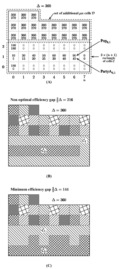
Figure 2: An illustration of the construction in the proof of Theorem 4 when the instance of the PARTITION problem is $\mathcal{A}=\{10,30,40,50,60,80,90\}$.

Let $\mu\geq 0$ be such that $\kappa=2+\mu n$ (we will later show that $\mu$ is at most the constant $\frac{6\varepsilon}{1-\varepsilon}$). Our rectilinear polygon $\mathcal{P}$, as illustrated in Fig. 2 (A), consists of a rectangle $\mathcal{C}=\left\{p_{i,j}\,|\,0\leq i\leq n,\,0\leq j\leq 2\right\}$ of size $3\times(n+1)$ with additional $\mu n$ cells attached to it in any arbitrary manner to make the whole figure a connected polygon without holes. For convenience, let $\mathcal{D}=\left\{p_{i,j}\,|\,p_{i,j}\notin\mathcal{C}\right\}$ be the set of the additional $\mu n$ cells. The relevant numbers for each cell are as follows:

$${\mathrm{Pop}}_{i,j}=\left\{\begin{array}[]{r l}\nicefrac{{\Delta}}{{2}},&\mbox{if $i=j=0$ or if $i=0,j=2$}\\ a_{j},&\mbox{if $i=1$ and $j<n$}\\ \Delta,&\mbox{if $p_{i,j}\in\mathcal{D}$}\\ 0,&\mbox{otherwise}\end{array}\right.\,\,\,\,\,\,\,\,\,\,{\mathrm{PartyA}}_{i,j}=\left\{\begin{array}[]{r l}\nicefrac{{\Delta}}{{2}},&\mbox{if $i=j=0$}\\ \nicefrac{{a_{j}}}{{2}},&\mbox{if $i=1$ and $j<n$}\\ \nicefrac{{3\Delta}}{{4}},&\mbox{if $p_{i,j}\in\mathcal{D}$}\\ 0,&\mbox{otherwise}\end{array}\right.$$

First, we show how to select a rational constant $\mu$ such that any integer $\kappa$ in the range $[\,2,\varepsilon|\mathcal{P}|\,]$ can be realized. Assume that $\kappa=\varepsilon^{\prime}|\mathcal{P}|\in[\,2,\varepsilon|\mathcal{P}|\,]$ for some $\varepsilon^{\prime}$. Since $|\mathcal{P}|=3(n+1)+\mu n$ the following calculations hold:

$$\kappa=2+\mu n=\varepsilon^{\prime}|\mathcal{P}|=\varepsilon^{\prime}(3(n+1)+\mu n)\,\equiv\,\mu=\frac{3\varepsilon^{\prime}(n+1)-2}{(1-\varepsilon^{\prime})n}<\frac{4\varepsilon^{\prime}}{1-\varepsilon^{\prime}}<\frac{4\varepsilon}{1-\varepsilon}$$

Claim 4.1 $\mathsf{Effgap}(p_{i,j})=0$ for each $p_{i,j}\in\mathcal{D}$, and moreover each $p_{i,j}\in\mathcal{D}$ must be a separate partition by itself in any $\kappa$-equipartition of $\mathcal{P}$.

Proof.  By straightforward calculation, $\mathsf{Effgap}(p_{i,j})=2\times\frac{3\Delta}{4}-\frac{3\Delta}{2}=0$. Since $\kappa=2+\mu n$ and ${\mathrm{Pop}}(\mathcal{P})=\sum_{p_{i,j}\in\mathcal{P}}{\mathrm{Pop}}_{i,j}=\Delta+\Delta+\mu n\Delta=(2+\mu n)\Delta$, each partition in any $\kappa$-equipartition of $\mathcal{P}$ must have a population of $\frac{{\mathrm{Pop}}(\mathcal{P})}{\kappa}=\Delta$ and thus each $p_{i,j}\in\mathcal{D}$ of population $\Delta$ must be a separate partition by itself. ❑

Using Claim 4.1 we can simply ignore all $p_{i,j}\in\mathcal{D}$ in the calculation of of efficiency gap of a valid solution of $\mathcal{P}$ and it follows that the total efficiency gap of a $\kappa$-equipartition of $\mathcal{P}$ is identical to that of a $2$-equipartition of $\mathcal{C}$. A proof of the theorem then follows provided we prove the following two claims.

     (soundness)

If the PARTITION problem does not have a solution then ${\mathsf{OPT}}_{2}(\mathcal{C})=\Delta$.

(completeness)

If the PARTITION problem has a solution then ${\mathsf{OPT}}_{2}(\mathcal{C})=0$.

Proof of soundness (refer to Fig. 2 (B))

Suppose that there exists a valid solution (i.e., a $2$-equipartition) $\mathcal{C}_{1},\mathcal{C}_{2}$ of Min-wvp₂ for $\mathcal{C}$ with $p_{0,0}\in\mathcal{C}_{1},p_{0,2}\in\mathcal{C}_{2}$, and let $\mathcal{A}^{\prime}=\left\{a_{j}\,|\,p_{1,j}\in\mathcal{C}_{1}\right\}$. Then,

$$\Delta=\frac{{\mathrm{Pop}}(\mathcal{C})}{2}={\mathrm{Pop}}_{0,0}+\sum_{p_{1,j}\in\mathcal{C}_{1}}{\mathrm{Pop}}_{1,j}=\frac{\Delta}{2}+\sum_{a_{j}\in\mathcal{A}^{\prime}}a_{j}\,\equiv\,\sum_{a_{j}\in\mathcal{A}^{\prime}}a_{j}=\frac{\Delta}{2}$$

and thus $\mathcal{A}^{\prime}$ is a valid solution of PARTITION, a contradiction!

Thus, assume that both $p_{0,0}$ and $p_{0,2}$ belong to the same partition, say $\mathcal{C}_{1}$. Then, since ${\mathrm{Pop}}_{0,0}+{\mathrm{Pop}}_{0,4}=\Delta=\frac{{\mathrm{Pop}}(\mathcal{C})}{2}$, every $p_{1,j}$ must belong to $\mathcal{C}_{2}$. Moreover, every $p_{i,j}\in\mathcal{C}$ with $\eta_{i,j}=0$ must belong to $\mathcal{C}_{1}$ since otherwise $\mathcal{C}_{1}$ will not be a connected region. This provides ${\mathrm{Pop}}(\mathcal{C}_{1})={\mathrm{Pop}}(\mathcal{C}_{2})=\Delta$, showing that $\mathcal{C}_{1},\mathcal{C}_{2}$ is indeed a valid solution (i.e., a $2$-equipartition) of Min-wvp₂ for $\mathcal{C}$. The total efficiency gap of this solution can be calculated as

$$\mathsf{Effgap}_{2}(\mathcal{C},\mathcal{C}_{1},\mathcal{C}_{2})=|\,\mathsf{Effgap}(\mathcal{C}_{1})+\mathsf{Effgap}(\mathcal{C}_{2})\,|\\ =\left|\,2\,{\mathrm{PartyA}}(\mathcal{C}_{1})-\frac{3}{2}{\mathrm{Pop}}(\mathcal{C}_{1})+2\,{\mathrm{PartyA}}(\mathcal{C}_{1})-\frac{3}{2}{\mathrm{Pop}}(\mathcal{C}_{1})\,\right|=\left|\,2\frac{\Delta}{2}-\frac{3}{2}\Delta+2\frac{\Delta}{2}-\frac{3}{2}\Delta\,\right|=\Delta$$

Proof of completeness (refer to Fig. 2 (C))

Suppose that there is a valid solution of $\mathcal{A}^{\prime}\subset\mathcal{A}$ of PARTITION and consider the two polygons

$$\mathcal{C}_{1}=\left\{p_{2,j}\,|\,0\leq j\leq n\right\}\cup\left\{p_{1,j}\,|\,a_{j}\in\mathcal{A}^{\prime}\right\},\,\,\,\,\,\,\mathcal{C}_{2}=\mathcal{C}\setminus\mathcal{C}_{1}$$

By straightforward calculation, it is easy to verify the following:

• ${\mathrm{Pop}}(\mathcal{C}_{1})=\sum_{a_{j}\in\mathcal{A}^{\prime}}a_{j}+\sum_{j=0}^{n}{\mathrm{Pop}}_{2,j}=\Delta$, ${\mathrm{Pop}}(\mathcal{C}_{2})=\sum_{a_{j}\notin\mathcal{A}^{\prime}}a_{j}+\sum_{j=0}^{n}{\mathrm{Pop}}_{2,j}=\Delta$, and thus $\mathcal{C}_{1},\mathcal{C}_{2}$ is a valid solution (i.e., a $2$-equipartition) of Min-wvp₂ for $\mathcal{C}$.

• $\mathsf{Effgap}_{2}(\mathcal{C},\mathcal{C}_{1},\mathcal{C}_{2})=0{\mathsf{OPT}}_{2}(\mathcal{C})=0$ since

  $$\mathsf{Effgap}_{2}(\mathcal{C},\mathcal{C}_{1},\mathcal{C}_{2})=|\,\mathsf{Effgap}(\mathcal{C}_{1})+\mathsf{Effgap}(\mathcal{C}_{2})\,|\\ =\left|\,2\,{\mathrm{PartyA}}(\mathcal{C}_{1})-\frac{3}{2}{\mathrm{Pop}}(\mathcal{C}_{1})+2\,{\mathrm{PartyA}}(\mathcal{C}_{1})-\frac{1}{2}{\mathrm{Pop}}(\mathcal{C}_{1})\,\right|\\ =\left|\,2\,\left(\frac{\Delta}{2}+\frac{\Delta}{4}\right)-\frac{3}{2}\Delta+2\frac{\Delta}{4}-\frac{1}{2}\Delta\,\right|=0$$

❑

5 Efficient Algorithms Under Realistic Assumptions

Although Theorem 4 seems to render the problem Min-wvp_κ intractable in theory, our empirical results show that the problem is computationally tractable in practice. This is because in real-life applications, many constraints in the theoretical formulation of Min-wvp_κ are often relaxed. For example:

(i) Restricting district shapes:

Individual partitions of the $\kappa$-equipartition of $\mathcal{P}$ may be restricted in shape. For example, $37$ states require their legislative districts to be reasonably compact and $18$ states require congressional districts to be compact [39].

(ii) Variations in district populations:

A partition $\mathcal{Q}_{1},\dots,\mathcal{Q}_{\kappa}$ of $\mathcal{P}$ is only approximately $\kappa$-equipartition, i.e., ${\mathrm{Pop}}(\mathcal{Q}_{1}),\dots,{\mathrm{Pop}}(\mathcal{Q}_{\kappa})$ are approximately, but not exactly, equal to $\nicefrac{{{\mathrm{Pop}}(\mathcal{P})}}{{\kappa}}$. For example, the usual federal standards require equal population as nearly as is practicable for congressional districts but allow more relaxed substantially equal population (e.g., no more than $10\%$ deviation between the largest and smallest district) for state and local legislative districts [39].

(iii) Bounding the efficiency gap measure away from zero:

A $\kappa$-equipartition $\mathcal{Q}_{1},\dots,\mathcal{Q}_{\kappa}$ of $\mathcal{P}$ is a valid solution only if $\mathsf{Effgap}_{\kappa}(\mathcal{P},\mathcal{Q}_{1},\dots,\mathcal{Q}_{\kappa})\geq\varepsilon{\mathrm{Pop}}(\mathcal{P})$ for some $0<\varepsilon<1$. Indeed, the authors that originally proposed the efficiency gap measure provided in [29, pp. 886-887] several reasons for not requiring $\mathsf{Effgap}_{\kappa}(\mathcal{P},\mathcal{Q}_{1},\dots,\mathcal{Q}_{\kappa})/{\mathrm{Pop}}(\mathcal{P})$ to be either zero or too close to zero.

In this section, we explore algorithmic implications of these types of relaxations of constraints for Min-wvp_κ.

5.1 The Case of Two Stable and Approximately Equal Partitions

This case considers constraints (ii) and (iii). The following definition of “near partitions” formalizes the concept of variations in district populations.

Definition 5 (Near partitions)

Let $\kappa\in\mathbb{N}$, and let $\mathcal{P}$ be an instance of Min-wvp_κ. Let $\phi\stackrel{{\scriptstyle\mathrm{def}}}{{=}}\mathcal{Q}_{i},\ldots,\mathcal{Q}_{\kappa}$ be such that $\mathcal{Q}_{1},\ldots,\mathcal{Q}_{\kappa}$ is a partition of $\mathcal{P}$, such that for each $i\in\{1,\ldots,\kappa\}$, we have

$$\left(\frac{1}{\kappa}-\delta\right)\cdot{\mathrm{Pop}}(\mathcal{P})\leq{\mathrm{Pop}}(\mathcal{Q}_{i})\leq\left(\frac{1}{\kappa}+\delta\right)\cdot{\mathrm{Pop}}(\mathcal{P}),$$

for some $\delta\geq 0$. Then we say that $\phi$ is a $\delta$-near partition.

The next definition of “stability” formalizes the concept of bounding away from zero the efficiency gap of each partition.

Definition 6 (Stability)

Let $\kappa\in\mathbb{N}$, let $\mathcal{P}$ be an instance of Min-wvp_κ, and let $\phi\stackrel{{\scriptstyle\mathrm{def}}}{{=}}\mathcal{Q}_{1},\ldots,\mathcal{Q}_{\kappa}$ be a partition for $\mathcal{P}$. We say that $\phi$ is $\gamma$-stable, for some $\gamma>0$, if for all $i\in\{1,\ldots,\kappa\}$, we have

$$\mathsf{Effgap}(\mathcal{Q}_{i})>\gamma\cdot{\mathrm{Pop}}(\mathcal{Q}_{i}).$$

Figure 3: The $10$-basic rectangles of a $32\times 32$ grid (left), the $10$-basic tree (middle), and a $10$-canonical solution (right).

Definition 7 (Canonical solution)

Let $\mathcal{P}$ be an instance of Min-wvp₂. Let $t\in\mathbb{N}$. Let $\mathcal{B}$ be the partition of $\mathcal{P}$ obtained as follows: We partition $\mathcal{P}$ into $\lfloor m/t\rfloor\cdot\rfloor n/t\rfloor$ rectangles, where each rectangle consists of the intersection of $t$ rows with $t$ columns, except possibly for the rectangles that are incident to the right-most and the bottom-most boundaries of $\mathcal{P}$. We refer to the rectangles in $\mathcal{B}$ as $t$-basic (see figure 3). Let $T$ be the set of cells consisting of the union of the left-most column of $\mathcal{P}$, the top row of $\mathcal{P}$, and for each $t$-basic rectangle $X$, the bottom row of $X$, and the right-most column of $X$, except for the cell that is next to the top cell of that column (see figure 3). We refer to $T$ as the $t$-basic tree For each $t$-basic rectangle $X$, we define its interior to be the set of cells in $X$ that are at distance at least $2$ from $T$. A solution $\phi\stackrel{{\scriptstyle\mathrm{def}}}{{=}}\mathcal{Z}_{1},\mathcal{Z}_{2}$ of $\mathcal{P}$ is called $t$-canonical if it satisfies the following properties.

(1) $T\subseteq Z_{1}$.

(2) Let $X$ be a $t$-basic rectangle, and let $X^{\prime}$ be its interior. For each $i\in\{1,2\}$, let $A_{i}$ be the set of connected components of $X^{\prime}\cap\mathcal{Z}_{i}$. Then, for each $Y\in A_{1}$, there exists a unique cell in $T_{1}$ that is adjacent to both $Y$ and $T$. Moreover, all other cells in $X\setminus(X^{\prime}\cup T)$ are in $\mathcal{Z}_{2}$ (see Figure 3).

Lemma 8

Let $\mathcal{P}$ be an instance of Min-wvp₂. Suppose that there are no empty cells and the maximum number of people in any cell of $\mathcal{P}$ is $C$. Let $\gamma>0$, and suppose that there exists a $\gamma$-stable solution $\phi\stackrel{{\scriptstyle\mathrm{def}}}{{=}}\mathcal{Q}_{1},\mathcal{Q}_{2}$ for $P$. Then, for any $\varepsilon>0$, at least one of the following conditions hold:

(1) Either $\mathcal{Q}_{1}$ or $\mathcal{Q}_{2}$ is contained in some $1/\varepsilon$-basic rectangle.

(2) There exists a $\lceil 1/\varepsilon\rceil$-canonical $\delta$-near solution $\phi^{\prime}=\mathcal{Q}^{\prime}_{1},\mathcal{Q}^{\prime}_{2}$ of $\mathcal{P}$, for some $\delta=O(\varepsilon C)$, such that for all $i\in\{1,2\}$, we have $|{\mathrm{PartyA}}(\mathcal{Q}_{i})-{\mathrm{PartyA}}(\mathcal{Q}_{i}^{\prime})|\leq O(C\varepsilon n+m)$, and $|{\mathrm{PartyB}}(\mathcal{Q}_{i})-{\mathrm{PartyB}}(\mathcal{Q}_{i}^{\prime})|\leq O(C\varepsilon nm)$.

Proof.  It suffices to show that if condition (1) does not hold, then condition (2) does. We define a partition $\phi^{\prime}\stackrel{{\scriptstyle\mathrm{def}}}{{=}}\mathcal{Q}^{\prime}_{1},\mathcal{Q}^{\prime}_{2}$ of $\mathcal{P}$ as follows. We initialize $\mathcal{Q}^{\prime}_{1}$ to be empty. Let $T$ be the $1/\varepsilon$-basic tree. We add $T_{1}$ to $\mathcal{Q}^{\prime}_{1}$. For each $1/\varepsilon$-basic rectangle $X$, let $X^{\prime}$ be its interior. For each $i\in\{1,2\}$, let $A_{i}$ be the set of connected components of $X^{\prime}\cap\mathcal{Q}_{1}$. Since $\phi$ is a valid solution, we have that $\mathcal{Q}_{1}$ is connected. Since condition (1) does not hold, it follows that $\mathcal{Q}_{1}$ intersects at least two $1/\varepsilon$-basic rectangles. Therefore, each component $W\in A_{1}$ must contain some cell $c_{W}$ on the boundary of $X^{\prime}$. By construction, $c_{W}$ must be incident to some cell $c_{W}^{\prime}$ that is incident to $T$. We add $c_{W}^{\prime}$ to $\mathcal{Q}^{\prime}_{1}$. Repeating this process for all basic rectangles, and for all components $W$ as above. Finally, we define $\mathcal{Q}^{\prime}_{2}=\mathcal{P}\setminus\mathcal{Q}^{\prime}_{1}$. This completes the definition of the partition $\phi^{\prime}\stackrel{{\scriptstyle\mathrm{def}}}{{=}}\mathcal{Q}^{\prime}_{1},\mathcal{Q}^{\prime}_{2}$ of $\mathcal{P}$. It remains to show that this is the desired solution.

First, we need to show that $\phi^{\prime}$ is a valid solution. To that end, it suffices to show that both $\mathcal{Q}^{\prime}_{1}$ and $\mathcal{Q}^{\prime}_{2}$ are connected. The fact that $\mathcal{Q}^{\prime}_{1}$ is connected follows directly from its construction. To show that $\mathcal{Q}^{\prime}_{2}$ is connected we proceed by induction on the construction of $\mathcal{Q}^{\prime}_{1}$. Initially, $\mathcal{Q}^{\prime}_{1}$ consists of just the cells in $T$, and thus its complement is clearly connected. When we consider a component $W$, we add $W\cup\{c^{\prime}_{W}\}$ to $\mathcal{Q}^{\prime}_{1}$. Since we add only a single cell that is incident to both $W$ and $\mathcal{Q}^{\prime}_{1}$, it follows inductively that $\mathcal{Q}^{\prime}_{1}$ remains simply connected (that is, it does not contain any holes), and therefore its complement remains connected. This concludes the proof that both $\mathcal{Q}^{\prime}_{1}$ and $\mathcal{Q}^{\prime}_{2}$ are connected, and therefore $\phi^{\prime}$ is a valid solution.

The solutions $\phi$ and $\phi^{\prime}$ can disagree only on cells that are not in the interior of any basic rectangle. All these cells are contained in the union of $O(\varepsilon m)$ rows and $(\varepsilon n)$ columns. Thus, the total number of voters in these cells is at most $O(C\varepsilon nm)$. It follows that for each $i\in\{1,2\}$, we have $|{\mathrm{PartyA}}(\mathcal{Q}_{i})-{\mathrm{PartyA}}(\mathcal{Q}_{i}^{\prime})|\leq O(C\varepsilon nm)$, and $|{\mathrm{PartyB}}(\mathcal{Q}_{i})-{\mathrm{PartyB}}(\mathcal{Q}_{i}^{\prime})|\leq O(C\varepsilon nm)$.

Since there are no empty cells, we have ${\mathrm{Pop}}(\mathcal{P})\geq nm$. It follows that for all $i\in\{1,2\}$, we have

$$|{\mathrm{Pop}}(\mathcal{Q}_{i})-{\mathrm{Pop}}(\mathcal{Q}^{\prime}_{i})|\leq O(C\varepsilon nm)\leq C\cdot\varepsilon\cdot{\mathrm{Pop}}(\mathcal{P}).$$

Thus $\phi^{\prime}$ is $\delta$-near, for some $\delta=O(\varepsilon C)$, which concludes the proof. ❑

Lemma 9

Let $\gamma>0$. Let $\mathcal{P}$ be an instance of Min-wvp₂. Suppose that there are no empty cells and the maximum number of people in any cell of $\mathcal{P}$ is $C$. Suppose that there exists a $\delta$-stable partition $\phi\stackrel{{\scriptstyle\mathrm{def}}}{{=}}\mathcal{Q}_{1},\mathcal{Q}_{2}$ of $P$. Then, for any fixed $\varepsilon>0$, there exists an algorithm which given $\mathcal{P}$ computes some $\delta$-near partition $\phi^{\prime}\stackrel{{\scriptstyle\mathrm{def}}}{{=}}\mathcal{Q}^{\prime}_{1},\mathcal{Q}^{\prime}_{2}$ of $\mathcal{P}$, for some $\delta=O(\varepsilon C)$, such that for all $i\in\{1,2\}$, we have $|{\mathrm{PartyA}}(\mathcal{Q}_{i})-{\mathrm{PartyA}}(\mathcal{Q}_{i}^{\prime})|\leq O(C\varepsilon nm)$, and $|{\mathrm{PartyB}}(\mathcal{Q}_{i})-{\mathrm{PartyB}}(\mathcal{Q}_{i}^{\prime})|\leq O(C\varepsilon nm)$, in time $2^{O(1/\varepsilon^{2})}(nmC)^{O(1)}$.

Proof.  We can check whether there exist a partition $\phi\stackrel{{\scriptstyle\mathrm{def}}}{{=}}\mathcal{Q}_{1},\mathcal{Q}_{2}$ satisfying the conditions, and such that either $\mathcal{Q}_{1}$ or $\mathcal{Q}_{1}$ is contained in the interior of a single $1/\varepsilon$-basic rectangle. This can be done by trying all $1/\varepsilon$-basic rectangles, and all possible subsets of the interior of each $1/\varepsilon$-basic rectangle, in time $(n/\varepsilon)(m/\varepsilon)2^{O(1/\varepsilon^{2})}=nm2^{O(1/\varepsilon^{2})}$.

It remains to consider the case where neither of $\mathcal{Q}_{1}$ and $\mathcal{Q}_{2}$ is contained in the interior of any $1/\varepsilon$-basic rectangle. It follows that condition (2) of Lemma 8 holds. That is, there exists some $\lceil 1/\varepsilon\rceil$-canonical $\delta$-near solution $\phi^{\prime}\stackrel{{\scriptstyle\mathrm{def}}}{{=}}\mathcal{Q}^{\prime}_{1},\mathcal{Q}^{\prime}_{2}$ of $\mathcal{P}$, for some $\delta=O(\varepsilon C)$, such that for all $i\in\{1,2\}$, we have $|{\mathrm{PartyA}}(\mathcal{Q}_{i})-{\mathrm{PartyA}}(\mathcal{Q}_{i}^{\prime})|\leq O(C\varepsilon n+m)$, and $|{\mathrm{PartyB}}(\mathcal{Q}_{i})-{\mathrm{PartyB}}(\mathcal{Q}_{i}^{\prime})|\leq O(C\varepsilon nm)$. We can compute such a partition $\phi^{\prime}$ via dynamic programming, as follows. Let $I$ be the union of the interiors of all $1/\varepsilon$-basic rectangles. By the definition of a canonical partition, it suffices to compute $\mathcal{Q}^{\prime}_{1}\cap I$ and $\mathcal{Q}^{\prime}_{2}\cap I$. Since $\mathcal{Q}^{\prime}_{2}\cap I=I\setminus(\mathcal{Q}^{\prime}_{1}\cap I)$, it suffices to compute $\mathcal{Q}^{\prime}_{1}\cap I$. Let $L_{\mathrm{PartyA}}={\mathrm{PartyA}}(\mathcal{Q}^{\prime}_{1}\cap I)$, and $L_{\mathrm{PartyB}}={\mathrm{PartyB}}(\mathcal{Q}^{\prime}_{1}\cap I)$. Clearly, $L_{\mathrm{PartyA}},L_{\mathrm{PartyB}}\in\{0,\ldots,Cnm\}$. Thus there are at most $O((nmC)^{2})$ different values for the pair $(L_{\mathrm{PartyA}},L_{\mathrm{PartyB}})$. We construct a dynamic programming table, containing one entry for each possible value for the pair $(L_{\mathrm{PartyA}},L_{\mathrm{PartyB}})$. Initially, all entries of the table are unmarked, except for the entry that corresponds to the pair $(0,0)$. We iteratively consider all $1/\varepsilon$-basic rectangles. When considering some $1/\varepsilon$-basic rectangle $X$, with interior $X^{\prime}$, we enumerate all possibilities for $Y=X^{\prime}\cap\mathcal{Q}^{\prime}_{1}$. There are $2^{O(1/\varepsilon^{2})}$ possibilities for $Y$. For each such possibility, we update the dynamic programming table by marking the position $(i+{\mathrm{PartyA}}(Y),j+{\mathrm{PartyB}}(Y))$, if the position $(i,j)$ is already marked from the previous iteration. The total running time is $2^{O(1/\varepsilon^{2})}(nmC)^{O(1)}$. ❑

Theorem 10

Let $\gamma>0$. Let $\mathcal{P}$ be an instance of Min-wvp₂. Suppose that there are no empty cells and the maximum number of people in any cell of $\mathcal{P}$ is $C$. Suppose that there exists a $\delta$-stable $\gamma$-near partition $\phi\stackrel{{\scriptstyle\mathrm{def}}}{{=}}\mathcal{Q}_{1},\mathcal{Q}_{2}$ of $P$. Then, for any fixed $\varepsilon>0$, there exists an algorithm which given $\mathcal{P}$ computes some $\delta$-near partition $\phi^{\prime}\stackrel{{\scriptstyle\mathrm{def}}}{{=}}\mathcal{Q}^{\prime}_{1},\mathcal{Q}^{\prime}_{2}$ of $\mathcal{P}$, for some $\delta=O(\varepsilon C)$, such that $\mathsf{Effgap}(\phi^{\prime})\leq(1+\varepsilon)\mathsf{Effgap}(\phi)$, in time $2^{O(1/\varepsilon^{2})}2^{O(C/\delta)^{2}}(nmC)^{O(1)}$.

Proof.  It follows from Lemma 9 by setting $\varepsilon=\min\{\varepsilon,O(\delta/C)\}$. ❑

5.2 The Case of Convex Shaped Partitions

This case encompasses constraint (i) since convexity has been used in gerrymandering studies such as [40] as a measure of compactness to examine how redistricting reshapes the geography of congressional districts. We recall that some $X\subseteq\mathbb{R}^{2}$ is called $y$-convex if for every vertical line $\ell$, we have that $X\cap\ell$ is either empty, or a line segment. We also say that a $\kappa$-partition ${\cal Q}_{1},\ldots,Q_{\kappa}$ of ${\cal P}$ is $y$-convex if for all $i\in\{1,\ldots,\kappa\}$, ${\cal Q}_{i}$ is $y$-convex.

Theorem 11

Let ${\cal P}$ be a rectilinear polygon realized in the $m\times n$ grid, and let $N={\mathrm{Pop}}({\cal P})$ be the total population on ${\cal P}$. There exists an algorithm for computing a $y$-convex $\kappa$-equipartition of ${\cal P}$ of minimum efficiency gap, with running time $N^{O(\kappa)}$. In particular, the running time is polynomial when the total population is polynomial and the total number of partitions is a constant.

Proof.  Let ${\cal P}^{*}={\cal Q}_{1}^{*},\ldots,{\cal Q}_{\kappa}^{*}$ be a $y$-convex $\kappa$-equipartition of ${\cal P}$ of minimum efficiency gap. For any $i\in\{1,\ldots,n\}$, let $C_{i}$ be the $i$-th column of ${\cal P}$. We observe that for all $i\in\{1,\ldots,n\}$, and for all $j\in\{1,\ldots,\kappa\}$, we have that ${\cal Q}^{*}_{j}\cap C_{i}$ is either empty, or consists of a single rectangle of width $1$. Let ${\cal C}_{i}$ be the set of all partitions of $C_{i}$ into exactly $\kappa$ (possibly empty) segments, each labeled with a unique integer in $\{1,\ldots,\kappa\}$. We further define

$$a^{*}_{i,j}={\mathrm{PartyA}}({\cal Q}_{j}^{*}\cap(C_{1}\cup\ldots\cup C_{i})),$$

and

$$b^{*}_{i,j}={\mathrm{PartyB}}({\cal Q}_{j}^{*}\cap(C_{1}\cup\ldots\cup C_{i})).$$

The algorithm proceeds via dynamic programming. For each $i\in\{1,\ldots,n\}$, let $I_{i}=\mathbb{N}^{2\kappa}\times{\cal S}_{i}$. Let $X_{i}=(a_{i,1},b_{i,1},\ldots,a_{i,\kappa},b_{i,\kappa},{\cal Z}_{i})\in I_{i}$. If $i=1$, then we say that $X_{i}$ is feasible if for all $j\in\{1,\ldots,\kappa\}$, the unique set $Y\in{\cal Z}_{1}$ labeled $j$ satisfies

$$a_{1,j}={\mathrm{PartyA}}(Y)\text{ and }b_{1,j}={\mathrm{PartyB}}(Y).$$

Otherwise, if $i>1$, we say that $X_{i}$ is feasible if the following holds: There exists some feasible $X_{i-1}=(a_{i-1,1},b_{i-1,1},\ldots,a_{i-1,\kappa},b_{i-1,\kappa},{\cal Z}_{i-1})\in I_{i-1}$, such that for all $j\in\{1,\ldots,\kappa\}$, we have that the unique set $Y\in{\cal Z}_{i}$ labeled $j$ satisfies

$$a_{i,j}=a_{i-1,j}+{\mathrm{PartyA}}(Y)\text{ and }b_{i,j}=b_{i-1,j}+{\mathrm{PartyB}}(Y).$$

For each $i\in\{1,\ldots,n\}$ we inductively compute the set ${\cal F}_{i}$ of all feasible $X_{i}\in I_{i}$. This can clearly be done in time $N^{O(\kappa)}$. It is immediate that for all $i\in\{1,\ldots,n\}$, there exists some $X_{i}\in I_{i}$ that achieves efficiency gap equal to the restriction of ${\cal P}^{*}$ on the union of the first $i$ columns. Thus, by induction on $i$, the algorithm computes a feasible solution with optimal efficiency gap. ❑

6 Experimental Results for Real Data on Four Gerrymandered States

To show that it is indeed possible in practice to solve the problem of minimization of the efficiency gap, we design a fast randomized algorithm based on the local search paradigm for this problem. Our algorithm starts with a given $\mathcal{Q}_{1},\dots,\mathcal{Q}_{\kappa}$ partition of the input state $\mathcal{P}$. Note that $\mathcal{Q}_{1},\dots,\mathcal{Q}_{\kappa}$ was only an approximate equipartition in the sense that the values ${\mathrm{Pop}}(\mathcal{Q}_{1}),\dots,{\mathrm{Pop}}(\mathcal{Q}_{\kappa})$ are as close to each other as practically possible but need not be exactly equal (cf. US Supreme Court ruling in Karcher v. Daggett $1983$). For designing alternate valid district plans, we therefore allow any partition $\mathcal{Q}^{\prime}_{1},\dots,\mathcal{Q}^{\prime}_{\kappa}$ of $\mathcal{P}$ such that, for every $j$, $\min_{1\leq i\leq\kappa}\left\{{\mathrm{Pop}}(\mathcal{Q}_{i})\right\}\leq{\mathrm{Pop}}(\mathcal{Q}^{\prime}_{j})\leq\max_{1\leq i\leq\kappa}\left\{{\mathrm{Pop}}(\mathcal{Q}_{i})\right\}$.

6.1 Input preprocessing

We preprocess the input map to generate an undirected unweighted planar graph ${\mathfrak{G}}=({\mathfrak{V}},{\mathfrak{E}})$. Each node in the graph corresponds to a planar subdivision of a county that is assigned to a district (or to an entire county if it is assigned to a district as a whole). Two nodes are connected by an edge if and only if they share a border on the map. Each node $v\in{\mathfrak{V}}$ has three corresponding numbers: ${\mathrm{PartyA}}(v)$ (total number of voters for Party A), ${\mathrm{PartyB}}(v)=$ (total number of voters for Party B), and ${\mathrm{Pop}}(v)={\mathrm{PartyA}}(v)+{\mathrm{PartyB}}(v)$ (total population in $v$). A district $\mathcal{Q}$ is then a connected sub-graph of ${\mathfrak{G}}$ with ${\mathrm{PartyA}}(\mathcal{Q})=\sum_{v\in\mathcal{Q}}{\mathrm{PartyA}}(v)$ and ${\mathrm{PartyB}}(\mathcal{Q})=\sum_{v\in\mathcal{Q}}{\mathrm{PartyB}}(v)$.

6.2 Availability and Format of Raw Data

Link to all data files for the three states used in the paper are available in http://www.cs.uic.edu/~dasgupta/gerrymander/index.html. Each data is an EXCEL spreadsheet. Explanations of various columns of the spreadsheet are as follows:

Column 1: District:

This column identifies the district number of the county in column 3.

Column 2: County_id:

Column 1 and column 2 together form an unique identifier for the counties in column 3. A county is identified by its County_id (column 2) and the District (column 1) it belongs to. This was specifically needed to identify and differentiate the counties that belonged to more than one district.

The software considers the counties belonging to different districts as separate entities.

Column 3: County:

This column contains the name of the county.

Column 4: Republicans:

This contains the total number of votes in favor of the Republican party (GOP) in the county identified by column 1 and column 2.

Column 4: Democrats:

This contains the total number of votes in favor of the Democratic party in the county identified by column 1 and column 2.

Column 5: Neighbors:

This column contains information about the “neighboring counties” of the given county. Neighboring counties represent the counties that share a boundary with the county identified by column 1 and column 2. Individual neighbors are separated by commas.

6.3 The Local-search Heuristic

Informally, our algorithm starts with the existing (possibly gerrymandered) districts and then repeatedly attempts to reassign counties (or parts of counties) into neighboring districts. This was done on a semi-random basis, and on average about $100$ iterations were carried out in each run. Each time a county (or a part of a county) was shifted, the efficiency gap was calculated to check if it was less than the prior efficiency gap. Exact details of our algorithm are shown in Fig. 4.

start with the current districts, say $\mathcal{Q}_{1},\dots,\mathcal{Q}_{\kappa}$

repeat $\mu$ times $(*$ $\mu$ was set to $100$ in actual run $*)$

select a random $r$ from the set $\{0,1,\dots,k\}$ for some $0<k<|V|$       $(*$ $k=20$ in actual run $*)$

select $r$ nodes $v_{1},\dots,v_{r}$ from ${\mathfrak{G}}$ at random       $(*$ Note that a node is a county or part of a county $*)$

$\mathsf{counties\_done}\leftarrow\emptyset$

for each $v_{i}$ do

if all neighbors of $v_{i}$ do not belong to the same district as $v_{i}$ then

if $v_{i}\notin\mathsf{counties\_done}$ then

add $v_{i}$ to $\mathsf{counties\_done}$

for every neighbor $v_{j}$ of $v_{i}$ do

if assigning $v_{i}$ to the district of $v_{j}$ produces no district with disconnected parts then

assign $v_{i}$ to the district of one of its neighbors

recalculate new districts, say $\mathcal{Q}^{\prime}_{1},\dots,\mathcal{Q}^{\prime}_{\kappa}$

if $\min_{1\leq i\leq\kappa}\left\{{\mathrm{Pop}}(\mathcal{Q}_{i})\right\}\leq{\mathrm{Pop}}(\mathcal{Q}^{\prime}_{j})\leq\max_{1\leq i\leq\kappa}\left\{{\mathrm{Pop}}(\mathcal{Q}_{i})\right\}$ for every $j$ then

if $\mathsf{Effgap}_{\kappa}(\mathcal{P},\mathcal{Q}^{\prime}_{1},\dots,\mathcal{Q}^{\prime}_{\kappa})<\mathsf{Effgap}_{\kappa}(\mathcal{P},\mathcal{Q}_{1},\dots,\mathcal{Q}_{\kappa})$ then

$\mathcal{Q}_{1}\leftarrow\mathcal{Q}^{\prime}_{1}$ ; $\mathcal{Q}_{2}\leftarrow\mathcal{Q}^{\prime}_{2}$ ; $\dots\dots$ ; $\mathcal{Q}_{\kappa}\leftarrow\mathcal{Q}^{\prime}_{\kappa}$

endif

endif

endif

endfor

endif

endif

endfor

endrepeat

Figure 4: A local search algorithm for computing efficiency gap. The algorithm was implemented using the PYTHON language.

One cannot provide any theoretical analysis of the randomized algorithm in Fig. 4 because no such analysis is possible (due to Theorem 4) as stated formally in the following lemma.

Lemma 12

Assuming $P\neq\mathsf{NP}$ (respectively, $RP\neq\mathsf{NP}$), there exists no deterministic local-search algorithms (respectively, randomized local-search algorithms) that reaches a solution with a finite approximation ratio in polynomial time starting at any non-optimal valid solution.

Proof.  This follows from the proof of Theorem 4 once observes that the specific instance of the Min-wvp_κ problem created in the reduction of the theorem has exactly one (trivial) non-optimal solution and every other valid solution is an optimal solution. ❑

6.4 Results and Implications

Our resulting software was tested on four electoral data for the $2012$ election of the (federal) house of representatives for the US states of Wisconsin [36, 35], Texas [38, 37], Virginia [33, 34] and Pennsylvania [31, 32]. Some summary statistics for these data are shown in Table 1. The results of running the local-search algorithm in Fig. 4 on the four real data-sets are tabulated in Table 2, and the corresponding maps are shown in Fig. 5–8. The results computed by our algorithm are truly outstanding: the final efficiency gap was lowered to $3.80\%$, $3.33\%$, $3.61\%$ and $8.64\%$ from $14.76\%$, $4.09\%$, $22.25\%$ and $23.80\%$ for Wisconsin, Texas, Virginia and Pennsylvania, respectively, in a small amount of time. Our empirical results clearly show that it is very much possible to design and implement a very fast algorithm that can “un-gerrymander” (with respect to the efficiency gap measure) the gerrymandered US house districts of three US states.

	Vote share		Number of Seats		Normalized efficiency gap
	Democrats	GOP	Democrats	GOP	(current)
	$\boldsymbol{\dfrac{{\mathrm{PartyA}}(\mathcal{P})}{{\mathrm{Pop}}(\mathcal{P})}}$	$\boldsymbol{\dfrac{{\mathrm{PartyB}}(\mathcal{P})}{{\mathrm{Pop}}(\mathcal{P})}}$			$\boldsymbol{\mathsf{Effgap}_{\kappa}(\mathcal{P},\dots\dots)/{\mathrm{Pop}}(\mathcal{P})}$
Wisconsin	$50.75\%$	$49.25\%$	$3$	$5$	$14.76\%$
Texas	$43.65\%$	$56.35\%$	$12$	$24$	$4.09\%$
Virginia	$51.96\%$	$48.04\%$	$4$	$7$	$22.25\%$
Pennsylvania	$50.65\%$	$49.35\%$	$5$	$13$	$23.80\%$

Table 1: Summary statistics for $2012$ election data for election of the (federal) house of representatives for the states of Texas, Wisconsin, Virginia and Pennsylvania.

A closer look at the new district maps shown in Fig. 5–8 also reveal the following interesting insights:

Seat gain vs. efficiency gap.

Lowering the efficiency gap from $15\%$ to $3.75\%$ for the state of Wisconsin did not affect the total seat allocation ($3$ democrats vs. $5$ republicans) between the two parties. Indeed, this further reinforces the assertion in [29] that the efficiency gap and partisan symmetry are different concepts, and thus fewer absolute difference of wasted votes does not necessarily lead to seat gains for the loosing party.

Compactness vs. efficiency gap.

The new district maps for the state of Virginia reveals an interesting aspect. Our new district map have fewer districts that are oddly shaped compared to the map used for the $2012$ election, even though minimizing wasted votes does not take into consideration shapes of districts.

How natural are gerrymandered districts?

Since our algorithm applies a sequence of carefully chosen semi-random perturbations to the original gerrymandered districts to drastically lower the absolute difference of wasted votes, one can hypothesize that the original gerrymandered districts are far from being a product of arbitrarily random decisions. However, to reach a definitive conclusion regarding this point, one would need to construct a suitable null model, which we do not have yet.

	Number of Seats					Normalized efficiency gap
	Original		New			$\boldsymbol{\mathsf{Effgap}_{\kappa}(\mathcal{P},\dots\dots)/{\mathrm{Pop}}(\mathcal{P})}\,\,\,\,\,\,\,\,\,\,\,\,$
	Democrats	GOP	Democrats	GOP		Original	New
Wisconsin	$3$	$5$	$3$	$5$		$14.76\%$	$3.80\%$
Texas	$12$	$24$	$12$	$24$		$4.09\%$	$3.33\%$
Virginia	$3$	$8$	$5$	$6$		$22.25\%$	$3.61\%$
Pennsylvania	$5$	$13$	$6$	$12$		$23.80\%$	$8.64\%$

Table 2: Redistricting results obtained by running the algorithm in Fig. 4 for the states of Texas, Wisconsin, Virginia and Pennsylvania in comparison to the $2012$ district plans.

Figure 5: The district maps of Wisconsin: (A) original [36] and (B) after applying our local search algorithm in Fig. 4.

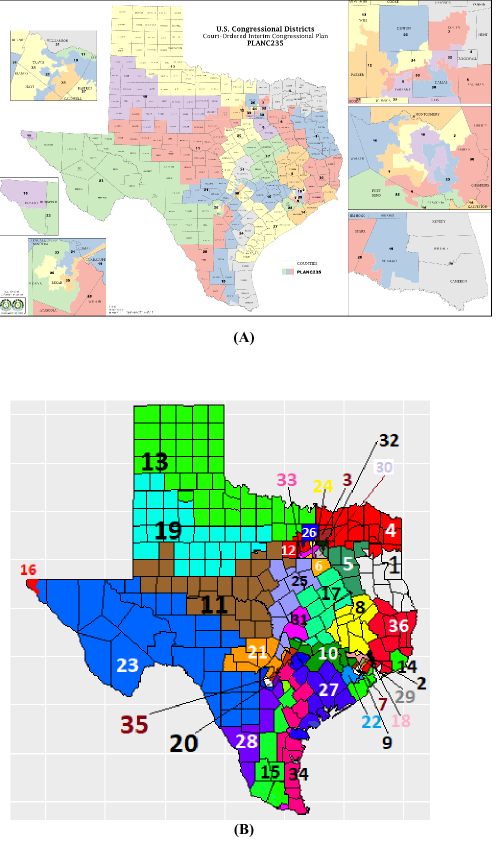
Figure 6: The district maps of Texas: (A) original [38] and (B) after applying our local search algorithm in Fig. 4.

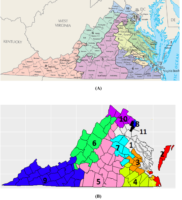
Figure 7: The district maps of Virginia: (A) original [34] and (B) after applying our local search algorithm in Fig. 4.

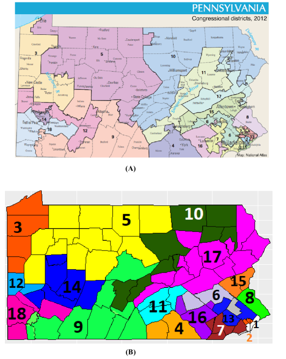
Figure 8: The district maps of Pennsylvania: (A) original [32] and (B) after applying our local search algorithm in Fig. 4.

7 Conclusion and future research

In this article we have performed algorithmic analysis of the recently introduced efficiency gap measure for gerrymandering both from a theoretical (computational complexity) as well as a practical (software development and testing on real data) point of view. The main objective of the paper was to provide a scientific analysis of the efficiency gap measure and to provide a crucial supporting hand to remove partisan gerrymandering should the US courts decide to recognize efficiency gap as at least a partially valid measure of gerrymandering. Of course, final words on resolving gerrymandering is up to the US judicial systems.

References

- [1] E. Aarts, J. K. Lenstra (Editors), Local Search in Combinatorial Optimization (Princeton University Press 2003).
- [2] N. Alon, J. H. Spencer, The Probabilistic Method (Wiley Inc., 2016).
- [3] M. Altman, A Bayesian approach to detecting electoral manipulation. Political Geography 21, 39-48 (2002).
- [4] J. L. Balcazar, J. Diaz, J. Gabarró, Structural Complexity I (Springer, 1995).
- [5] K. P. Burnham, D. R. Anderson, Model Selection and Multimodel Inference (Springer, 2002).
- [6] E. B. Cain. Simple v. complex criteria for partisan gerrymandering: a comment on Niemi and Grofman. UCLA Law Review 33, 213-226 (1985).
- [7] J. Chen, J. Rodden, Cutting through the thicket: redistricting simulations and the detection of partisan gerrymanders. Election Law Journal 14(4), 331-345 (2015).
- [8] W. K. T. Cho, Y. Y. Liu, Toward a talismanic redistricting tool: a computational method for identifying extreme redistricting plans. Election Law Journal: Rules, Politics, and Policy 15(4), 351-366 (2016).
- [9] S. A. Cook, The complexity of theorem proving procedures. In Annual ACM Symposium on the Theory of Computing, 151-158 (1971).
- [10] B. DasGupta, J. Liang, Models and Algorithms for Biomolecules and Molecular Networks (John Wiley & Sons, 2016).
- [11] Davis v. Bandemer, 478 US 109 (1986).
- [12] D. L. Faigman, To have and have not: assessing the value of social science to the law as science and policy. Emory Law Journal 38, 1005-1095 (1989).
- [13] B. Fifield, M. Higgins, K. Imai, A. Tarr, A new automated redistricting simulator using markov chain monte carlo. (manuscript, Princeton University, Princeton, NJ, 2018; available from https://imai.princeton.edu/research/files/redist.pdf).
- [14] W. M. Fitch, Toward defining the course of evolution: minimum change for a specified tree topology. Systematic Zoology 20(4), 406-416 (1971).
- [15] M. R. Garey, D. S. Johnson, Computers and Intractability - A Guide to the Theory of NP-Completeness (W. H. Freeman & Co., San Francisco, CA, 1979).
- [16] A. Gelman, G. King, A unified method of evaluating electoral systems and redistricting plans. American Journal of Political Science 38(2), 514-554 (1994).
- [17] Gill v. Whitford, US Supreme Court docket no -, decision pending (2017)
- [18] S. Jackman, Measuring electoral bias: Australia, 1949-93. British Journal of Political Science 24(3), 319-357 (1994).
- [19] G. Herschlag, R. Ravier, J. C. Mattingly, Evaluating Partisan Gerrymandering in Wisconsin. arXiv:1709.01596 (2017).
- [20] R. M. Karp, Reducibility Among Combinatorial Problems. In R. E. Miller and J.W. Thatcher (editors), Complexity of Computer Computations 85-103 (1972).
- [21] League of united latin american citizens v. Perry, 548 US 399 (2006).
- [22] Y. Y. Liu, K. Wendy, T. Cho, S. Wang, PEAR: a massively parallel evolutionary computational approach for political redistricting optimization and analysis. Swarm and Evolutionary Computation 30, 78-92 (2016).
- [23] E. McGhee, Measuring partisan bias in single-member district electoral systems. Legislative Studies Quarterly 39(1), 55-85 (2014).
- [24] R. Motwani, P. Raghavan, Randomized Algorithms (Cambridge University Press, 1995).
- [25] R. G. Niemi, B. Grofman, C. Carlucci, T. Hofeller, Measuring compactness and the role of a compactness standard in a test for partisan and racial gerrymandering. Journal of Politics 52(4), 1155-1181 (1990).
- [26] R. G. Niemi, J. Deegan, A theory of political districting. The American Political Science Review 72(4), 1304-1323 (1978).
- [27] “Ockham’s razor”, Encyclopædia Britannica (2010).
- [28] J. E. Ryan, The limited influence of social science evidence in modern desegregation cases. North Carolina Law Review 81(4), 1659-1702 (2003).
- [29] N. Stephanopoulos, E. McGhee, Partisan gerrymandering and the efficiency gap. University of Chicago Law Review 82(2), 831-900 (2015).
- [30] J. Thoreson, J. Liittschwager, Computers in behavioral science: legislative districting by computer simulation. Behavioral Science 12, 237-247 (1967).
- [31] http://elections.nbcnews.com/ns/politics/2012/Pennsylvania
- [32] https://en.wikipedia.org/wiki/Pennsylvania%27s_congressional_districts#/media/File:Pennsylvania_Congressional_Districts,_113th_Congress.tif
- [33] http://elections.nbcnews.com/ns/politics/2012/Virginia
- [34] http://www.virginiaplaces.org/government/congdist.html
- [35] http://elections.nbcnews.com/ns/politics/2012/Wisconsin
- [36] https://en.wikipedia.org/wiki/Wisconsin%27s_congressional_districts.
- [37] http://elections.sos.state.tx.us/elchist164_raceselect.htm
- [38] http://www.unityparty.us/State/texas-congressional-districts.htm
- [39] http://redistricting.lls.edu/where.php.
- [40] “Redrawing the map on redistricting 2010: a national study” (Azavea White Paper, © Azavea, 2009; https://cdn.azavea.com/com.redistrictingthenation/pdfs/Redistricting_The_Nation_White_Paper_2010.pdf).
- [41] https://en.wikipedia.org/wiki/Virginia’s_congressional_districts, see also https://www.onevirginia2021.org/