A Computational Study of the Collapse of
a Cloud with $12^{\prime}500$ Gas Bubbles in a Liquid

Abstract

We investigate the process of cloud cavitation collapse through large-scale simulation of a cloud composed of $12^{\prime}500$ gas bubbles. A finite volume scheme is used on a structured Cartesian grid to solve the Euler equations, and the bubbles are discretized by a diffuse interface method. We investigate the propagation of the collapse wave front through the cloud and provide comparisons to simplified models. We analyze the flow field to identify each bubble of the cloud and its associated microjet. We find that the oscillation frequency of the bubbles and the velocity magnitude of the microjets depend on the local strength of the collapse wave and hence on the radial position of the bubbles in the cloud. At the same time, the direction of the microjets is influenced by the distribution of the bubbles in its vicinity. Finally, an analysis of the pressure pulse spectrum shows that the pressure pulse rate is well captured by an exponential law.

I Introduction

Cavitation, i.e., the growth and rapid collapse of bubbles in a liquid subjected to large pressure variations, is often associated with damage on engineering devices such as marine propellers, hydroelectric turbines and fuel injectors Escaler:2006 ; Kumar:2010 ; Mitroglou:2017 . At the same time, the destructive power of cavitation is harnessed for non-invasive biomedical procedures such as kidney stone lithotripsy, drug delivery and tissue ablation histotripsy Ikeda:2006 ; Coussios:2008 ; Xu:2008 . The collapse of large numbers of bubbles (“clouds”) is among the most damaging types of cavitation, resulting in impulsive loads of high amplitude and short duration on surfaces. Such loads may cause local damage to the material known as cavitation erosion, largely attributed to the collapse of individual bubbles near the surface Kim:2014 .

Cloud cavitation collapse has been investigated both experimentally and numerically. Experiments have studied the collapse of a cloud of bubbles via the formation of an inward propagating shock wave and the geometric focusing of this shock at the center of the cloud Morch:1980 . Experimental measurements with hydrofoils subjected to cloud cavitation, conducted in Reisman:1998 , showed that very large pressure pulses occur within the cloud and are radiated outward during the collapse process. A technique developed in Bremond:2006 allowed for controlling the bubble distance within a two-dimensional cloud and thus ensured reproducibility of the cavitation events. The study revealed the shielding effect of the outer bubbles and showed the microjet formation. The final stage of the collapse of a hemispherical cloud near a solid surface was investigated using ultra high-speed photography in Brujan:2011 . Cloud cavitation in a water jet, including erosion tests, was examined in Yamamoto:2016 . Various numerical studies were also reported in literature; for instance, early ones assuming a potential flow in the liquid in Chahine:1992 ; Wang:1999 . The recently presented study in Ma:2015 used an Euler-Lagrange approach, combining the Navier-Stokes equations with subgrid-scale spherical bubbles governed by a Rayleigh-Plesset-like equation, to investigate spherical clouds collapsing near a rigid wall. A similar approach was applied in Chahine:2014c to study the impulsive loads generated by a cloud with $400$ bubbles under an imposed oscillating pressure field. Resolved and deforming bubbles were considered in Peng:2015 ; Adams:2013 ; Tiwari:2015 ; Sukys:2017 . A two-dimensional simulation of the collapse of a small cluster with 7 bubbles in an incompressible liquid using a front tracking method was presented in Peng:2015 . The collapse dynamics of a cloud composed of $125$ vapor bubbles with random radii was studied in Adams:2013 while  Tiwari:2015 reported the evolution of a hemispherical cloud of $50$ air bubbles. A comparison with the results of a homogeneous-mixture model and a coupled system of Rayleigh-Plesset-like equations revealed that both simplified models provided a qualitatively different prediction of the pressure field. A recent study  Sukys:2017 addressed uncertainty quantification for the collapse of clouds with $500$ randomly located gas bubbles. The goal of this paper is to advance the state of the art in studies of cloud cavitation collapse by simulating thousands of bubbles and studying their collective interactions.

Numerical methods for multicomponent flow that resolve both components on the computational grid may be classified into single-fluid and two-fluid approaches. In two-fluid methods, each component is governed by an individual set of conservation equations for mass, momentum and energy, and discontinuities at the interface are treated explicitly Fedkiw:1999 ; Hu:2009 ; Lauer:2012 ; Xu:2017 . In contrast, single-fluid methods, such as the diffuse interface method Allaire:2002 ; Saurel:1999a ; Saurel:2009 ; Tiwari:2013 introduce a zone around each interface where the transition from one component to the other is smeared over a few grid cells. In this context, single-fluid models present a compromise between accuracy and computational efficiency; that is, both components are explicitly distinguished, while the same numerical scheme can be used throughout the computational domain. This feature renders diffuse interface methods particularly appropriate for the large-scale simulation of flow problems with thousands of bubbles, as demonstrated by the compressible multicomponent flow solver presented in Rossinelli:2013 which showed a throughput of up to $7\cdot 10^{11}$ computational cells per second on $96$ racks of the IBM Sequoia.

Here, we employ an extended version of this compressible multicomponent flow solver to simulate the collapse process of a cloud of $12^{\prime}500$ resolved gas bubbles. The number of bubbles in the present simulation is up to two orders of magnitude larger than the ones considered in previous studies. Clouds of this size recover the separation of scales, i.e., a cloud of large extent formed by small bubbles. Therefore, the present cloud complies with the assumptions of simplified models for the propagation of the pressure wave resulting from the cloud collapse. At the same time, the large bubble count enables reliable statistics on the behavior of the individual bubbles and their associated microjets. Furthermore, the present simulation provides the data necessary to compile the pressure pulse spectrum of cloud cavitation collapse, in terms of the collective effect of individual bubble collapses.

The paper is organized as follows: Sec. II summarizes the governing equations together with the computational method and presents the setup of the cloud collapse problem. Sec. III reports on the cloud collapse dynamics from a macroscopic point of view. In Sec. IV, the dynamical behavior of the bubbles and their associated microjets are analyzed. The generated pressure pulse spectrum is examined in Sec. V. Sec. VI concludes the study.

II Governing equations and computational approach

In the following, we summarize the governing equations, the employed numerical scheme and the setup of the cloud collapse problem. The simulation presented in this study is conducted using the open source software Cubism-MPCF Rossinelli:2013 ; Hadjidoukas:2015b and cubism_link for download. The reader is referred to Rasthofer:2017 for the verification and validation of the compressible multicomponent flow solver in two-component shock-tube problems and for single-bubble collapse. A quantitative comparison to the solution of a coupled system of Rayleigh-Plesset-like equations for smaller clouds of 5 to 630 bubbles is presented in Rasthofer:2017b .

II.1 Governing equations

We study cloud cavitation collapse through the evolution of gas (air) bubbles in a liquid (water). The two components (water and air) are assumed immiscible and are captured by the diffuse interface method for compressible multicomponent flows. The present investigation involves the collapse of highly non-spherical bubbles that come along with strong microjets. In the case of strong microjets, inertia forces dominate the collapse process while viscous effects and surface tension may be considered negligible; see Betney:2015 . Hence, we adopt the Euler equations consisting of the mass conservation equations for each component, conservation equations for momentum and total energy in mixture- (or single-)fluid formulation and a transport equation for the volume fraction of one of the two components:

$$\frac{\partial\alpha_{1}\rho_{1}}{\partial t}+\nabla\cdot{\left(\alpha_{1}\rho_{1}\mathbf{u}\right)} =0,$$ (1)

$$\frac{\partial\alpha_{2}\rho_{2}}{\partial t}+\nabla\cdot{\left(\alpha_{2}\rho_{2}\mathbf{u}\right)} =0,$$ (2)

$$\frac{\partial\left(\rho\mathbf{u}\right)}{\partial t}+\nabla\cdot{\left(\rho\mathbf{u}\otimes\mathbf{u}+p\mathbf{I}\right)} =\mathbf{0},$$ (3)

$$\frac{\partial E}{\partial t}+\nabla\cdot{\left(\left(E+p\right)\mathbf{u}\right)} =0,$$ (4)

$$\frac{\partial\alpha_{2}}{\partial t}+\mathbf{u}\cdot\nabla{\alpha_{2}} =K\,\nabla\cdot{\mathbf{u}},$$ (5)

where

$$K=\frac{\alpha_{1}\alpha_{2}(\rho_{1}c_{1}^{2}-\rho_{2}c_{2}^{2})}{\alpha_{1}\rho_{2}c_{2}^{2}+\alpha_{2}\rho_{1}c_{1}^{2}};$$ (6)

see Murrone:2005 ; Perigaud:2005 for derivation. In Eqs. (1)-(5), $\mathbf{u}$ denotes the velocity, $p$ the pressure, $\mathbf{I}$ the identity tensor, $\rho$ the (mixture) density, $E$ the (mixture) total energy $E=\rho e+1/2\rho(\mathbf{u}\cdot\mathbf{u})$, where $e$ is the (mixture) specific internal energy. Moreover, $\rho_{k}$, $\alpha_{k}$ and $c_{k}$ with $k\in\{1,2\}$ are density, volume fraction and speed of sound of the two components. It holds that $\alpha_{1}+\alpha_{2}=1$ as well as $\rho=\alpha_{1}\rho_{1}+\alpha_{2}\rho_{2}$ and $\rho e=\alpha_{1}\rho_{1}e_{1}+\alpha_{2}\rho_{2}e_{2}$ for the mixture quantities. The source term on the right-hand side of the transport equation for $\alpha_{2}$ was originally derived in Kapila:2001 and is non-zero within the diffuse interface only. It allows for treating the interface zone as a compressible, homogeneous mixture of gas and liquid by capturing the reduction of the gas volume fraction when a compression wave travels across the mixing region and the increase for an expansion wave. As shown in Tiwari:2013 ; Rasthofer:2017 , the inclusion of this term notably increases the accuracy and lowers the resolution requirements. Moreover, it allows for a smooth transition to a homogeneous mixture model, if the resolution limit is reached by a collapsed bubble.

The system of Eqs. (1)-(5) is closed by the stiffened equation of state Menikoff:1989 :

$$p=\left(\gamma_{k}-1\right)\rho_{k}e_{k}-\gamma_{k}p_{\mathrm{c},k},$$ (7)

where isobaric closure is assumed Perigaud:2005 . The speed of sound is then given by

$$\rho_{k}c_{k}^{2}=\gamma_{k}\left(p+p_{\mathrm{c},k}\right).$$ (8)

The material parameters $\gamma_{k}$ and $p_{\mathrm{c},k}$ are assumed constant. Here, the values of Tiwari:2015 ; Saurel:1999a are used, which are given by $\gamma_{1}=4.4$ and $p_{\mathrm{c},1}=6.0\cdot 10^{2}\>\mathrm{MPa}$ for water and $\gamma_{2}=1.4$ and $p_{\mathrm{c},2}=0.0\>\mathrm{MPa}$ for air.

II.2 Numerical method

The system of governing equations (1)-(5) is expressed in a quasi-conservative form as

$$\frac{\partial\mathbf{Q}}{\partial t}+\nabla\cdot{\mathbf{F}}=\mathbf{R},$$ (9)

where $\mathbf{Q}=(\alpha_{1}\rho_{1},\alpha_{2}\rho_{2},\rho{\mathbf{u}},E,\alpha_{2})^{\mathrm{T}}$. The vector $\mathbf{F}=(\mathbf{F}^{(x)},\mathbf{F}^{(y)},\mathbf{F}^{(z)})^{\mathrm{T}}$ combines the fluxes $\mathbf{F}^{(x)}=(\alpha_{1}\rho_{1}u_{x},\alpha_{2}\rho_{2}u_{x},\rho u_{x}^{2}+p,\rho u_{y}u_{x},\rho u_{z}u_{x},(E+p)u_{x},\alpha_{2}u_{x})^{\mathrm{T}}$, $\mathbf{F}^{(y)}=(\alpha_{1}\rho_{1}u_{y},\alpha_{2}\rho_{2}u_{y},\rho u_{x}u_{y},\rho u_{y}^{2}+p,\rho u_{z}u_{y},(E+p)u_{y},\alpha_{2}u_{y})^{\mathrm{T}}$ and $\mathbf{F}^{(z)}=(\alpha_{1}\rho_{1}u_{z},\alpha_{2}\rho_{2}u_{z},\rho u_{x}u_{z},\rho u_{y}u_{z},\rho u_{z}^{2}+p,(E+p)u_{z},\alpha_{2}u_{z})^{\mathrm{T}}$. The right-hand-side vector $\mathbf{R}=(0,0,0,0,0,0,(K+\alpha_{2})\,\nabla\cdot{\mathbf{u}})^{\mathrm{T}}$ is zero except for the last component which comprises the source term of Eq. (5) and a contribution obtained from reformulating its convective term.

We solve Eq. (9) using a Godunov-type finite volume method on a uniform Cartesian grid. The choice of a uniform Cartesian grid enables the exploitation of High Performance Computing (HPC) architectures Rossinelli:2013 .The numerical fluxes at the cell faces are computed by an HLLC approximate Riemann solver, originally introduced for single-phase flow in Toro:1994 and more recently extended to multicomponent flows in Johnsen:2006 ; Tiwari:2013 ; Coralic:2014 . The fluxes are based on the primitive variables $\mathbf{u}$, $p$, $\alpha_{1}\rho_{1}$, $\alpha_{2}\rho_{2}$ and $\alpha_{2}$ at the cell faces, which are reconstructed from the cell average values using a shock-capturing third-order WENO scheme Jiang:1996 . Primitive variables are used for reconstruction to prevent numerical instabilities at the interface  Johnsen:2006 ; Karni:1994 . The approach suggested in Johnsen:2006 is adopted for the application of the HLLC Riemann solver to the evolution of $\alpha_{2}$. In summary, the resulting semi-discrete system reads as

$$\frac{d\mathbf{V}(t)}{dt} =\mathcal{L}(\mathbf{V}(t)),$$ (10)

where $\mathbf{V}$ denotes the vector of cell average values and $\mathcal{L}(\cdot)$ the spatially-discrete forms of divergence and source term in Eq. (9). Eq. (10) is discretized in time by a Total Variation Diminishing (TVD), low-storage, explicit third-order Runge-Kutta scheme  Gottlieb:1998 with a the time step dictated by the Courant-Friedrichs-Lewy (CFL) condition.

II.3 Cloud setup

We investigate an initially spherical cloud of radius $R_{\mathrm{C}}=45\>\mathrm{mm}$, composed of $n_{\mathrm{B}}=12^{\prime}500$ spherical bubbles of radius $R_{\mathrm{B}_{i}}$ with $i\in{1,...,n_{\mathrm{B}}}$. The cloud is generated by randomly positioning bubbles within a sphere of radius $R_{\mathrm{C}}$ using a uniform distribution and subject to the constraint that the minimum distance between the surfaces of any two bubbles is greater than $d_{\mathrm{G}}=0.4\>\mathrm{mm}$. The radius of the bubbles is chosen in the range $[R_{\mathrm{B,min}},R_{\mathrm{B,max}}]$ using a log-normal probability distribution. The minimum and maximum bubble radii values, $R_{\mathrm{B,min}}=0.5\>\mathrm{mm}$ and $R_{\mathrm{B,max}}=1.25\>\mathrm{mm}$, are based on the respective values suggested in Adams:2013 ; Tiwari:2015 . A two-dimensional sketch of the cloud setup is shown in Fig. 1.

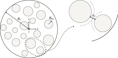
Figure 1: Sketch of spherical cloud with radius $R_{\mathrm{C}}$ composed of bubbles with radius $R_{\mathrm{B}}$ (left) as well as close-up of two bubbles separated by distance $d_{\mathrm{G}}$ (right).

The bubble cloud is characterized by the gas volume fraction $\alpha_{\mathrm{C}}$ and the cloud interaction parameter $\beta_{\mathrm{C}}$, defined as

$$\alpha_{\mathrm{C}}=\frac{1}{R_{\mathrm{C}}^{3}}\sum\limits_{i=1}^{n_{\mathrm{B}}}R_{\mathrm{B}_{i}}^{3},$$ (11)

$$\beta_{\mathrm{C}}=\alpha_{\mathrm{C}}\left(\frac{R_{\mathrm{C}}}{R_{\mathrm{B,avg}}}\right)^{2},$$ (12)

where

$$R_{\mathrm{B,avg}}=\frac{1}{n_{\mathrm{B}}}\sum_{i=1}^{n_{\mathrm{B}}}R_{\mathrm{B}_{i}}$$ (13)

denotes the average bubble radius. Higher $\beta_{\mathrm{C}}$ values indicate stronger interactions among the bubbles  Wang:1999 ; Brennen:1998 . For the present cloud, $\alpha_{\mathrm{C}}=4.9\%$, $\beta_{\mathrm{C}}=208$, and $R_{\mathrm{B,avg}}=0.69\>\mathrm{mm}$. Fig. 2 shows a histogram of the distribution of the bubble radius and a visualization of the generated cloud.

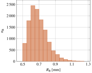
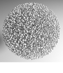
Figure 2: Distribution of bubble radius (left) and rendering of the initial cloud (right).

The cloud is centered in a cubic computational domain of size $6R_{\mathrm{C}}\times 6R_{\mathrm{C}}\times 6R_{\mathrm{C}}$. The domain is uniformly discretized using $6144\times 6144\times 6144$ cells, leading to $R_{\mathrm{B,min}}/h=11.38$ for the minimum bubble resolution and $R_{\mathrm{B,max}}/h=28.44$ for the maximum bubble resolution, where the cell length is denoted by $h$. Initially, a zero velocity field is assumed. The density of water is set to $\rho_{1}(\mathbf{x},t=0)=\rho_{1}(0)=1000.0\>\mathrm{kg/m^{3}}$ and of air to $\rho_{2}(0)=1.0\>\mathrm{kg/m^{3}}$. Moreover, a smoothed initial pressure field Tiwari:2015 is used which is essential in order to attenuate the emission of spurious pressure waves caused by the initial conditions. The bubble and liquid pressure in the sphere defining the cloud is set to $p_{\mathrm{C}}=0.1\>\mathrm{MPa}$ and the ambient pressure to $p_{\infty}=1.0\>\mathrm{MPa}$. Following  Tiwari:2015 , the initial pressure field in the liquid outside of the cloud is then obtained via

$$p(\mathbf{x},t=0)=\begin{cases}p_{\mathrm{C}}\quad&\text{if}\;\|\mathbf{x}-\mathbf{x}_{\mathrm{C}}\|\leq R_{\mathrm{C}},\\ p_{\mathrm{C}}+\mathrm{tanh}\left(\frac{\|\mathbf{x}-\mathbf{x}_{\mathrm{C}}\|-R_{\mathrm{C}}}{\lambda}\right)\left(p_{\infty}-p_{\mathrm{C}}\right)\quad&\text{otherwise},\end{cases}$$ (14)

where $\mathbf{x}_{\mathrm{C}}$ denotes the center of the cloud. Parameter $\lambda$ defines how fast the pressure increases from the cloud surface to the ambient and is set to $50\>\mathrm{mm}$. Non-reflecting, characteristic-based conditions Thompson:1987 ; Thompson:1990 ; Poinsot:1992 are applied at the boundaries of the computational domain. Additionally, we impose the ambient pressure $p_{\infty}$ in the far-field by adding the term $C_{\mathrm{bc}}(p-p_{\infty})$ to the incoming wave Rudy:1980 . Coefficient $C_{\mathrm{bc}}=\sigma(1-\mbox{{Ma}}^{2})c_{1}/\ell\approx\sigma c_{1}/\ell$ depends on a characteristic length $\ell=3R_{\mathrm{C}}$, the speed of sound $c_{1}$ in the liquid at the boundary, the Mach number Ma at the boundary, which is assumed negligible, and a user-defined parameter $\sigma=0.75\>\mathrm{s}$. Moreover, the CFL number is set to $0.3$.

III Cloud collapse dynamics

In this section, the cloud cavitation collapse is examined from a macroscopic point of view without considering the dynamics of the individual bubbles. The temporal evolution of characteristic quantities is provided together with visualizations of the collapsing cloud. Subsequently, the propagation of the collapse wave through the cloud is analyzed and compared to predictions by simplified models.

III.1 Temporal evolution and visualizations

We quantify the cloud collapse process through the temporal evolution of a number of local and global quantities. Fig. 3 shows the development of the gas volume $V_{2}/V_{2}(0)$, the point-wise maximum pressure $p_{\mathrm{max}}/p_{\mathrm{peak}}$ within the computational domain, the average pressure $p_{\mathrm{C}}/p_{\mathrm{C,peak}}$ within the cloud, the average pressure $p_{\mathrm{S}}/p_{\mathrm{S,peak}}$ within a sensor at the center of the cloud, further described below, and the total kinetic energy $E_{\mathrm{kin,C}}/E_{\mathrm{kin,C,peak}}$ within the cloud. All quantities are normalized by their peak (i.e., maximum) values. The symbols on top of the curve for the gas volume coincide with the time instants for which three-dimensional visualizations of the cloud together with the pressure iso-surface at $p_{\text{iso}}=0.15\>\mathrm{MPa}$ are shown in Fig. 4 and numerical schlieren of the pressure field in the $xy$-plane at $z=0$ in Fig. 5. The last two symbols correspond to the time of peak pressure $p_{\mathrm{S,peak}}$ within the sensor and the time of minimum gas volume, respectively. The remaining symbols are spaced evenly between $t=0$ and the time of occurrence of $p_{\mathrm{S,peak}}$.

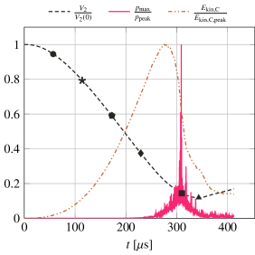
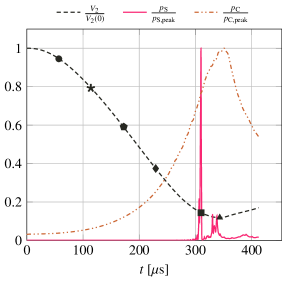
Figure 3: Temporal evolution of gas volume $V_{2}/V_{2}(0)$ together with point-wise maximum pressure $p_{\mathrm{max}}/p_{\mathrm{peak}}$ within domain and average kinetic energy $E_{\mathrm{kin,C}}/E_{\mathrm{kin,C,peak}}$ within cloud (left) as well as $V_{2}/V_{2}(0)$ together with average pressure $p_{\mathrm{C}}/p_{\mathrm{C,peak}}$ within cloud and average pressure $p_{\mathrm{S}}/p_{\mathrm{S,peak}}$ within sensor at cloud center (right). All quantities are normalized by their peak values. Symbols mark time instants for three-dimensional visualizations and numerical schlieren.

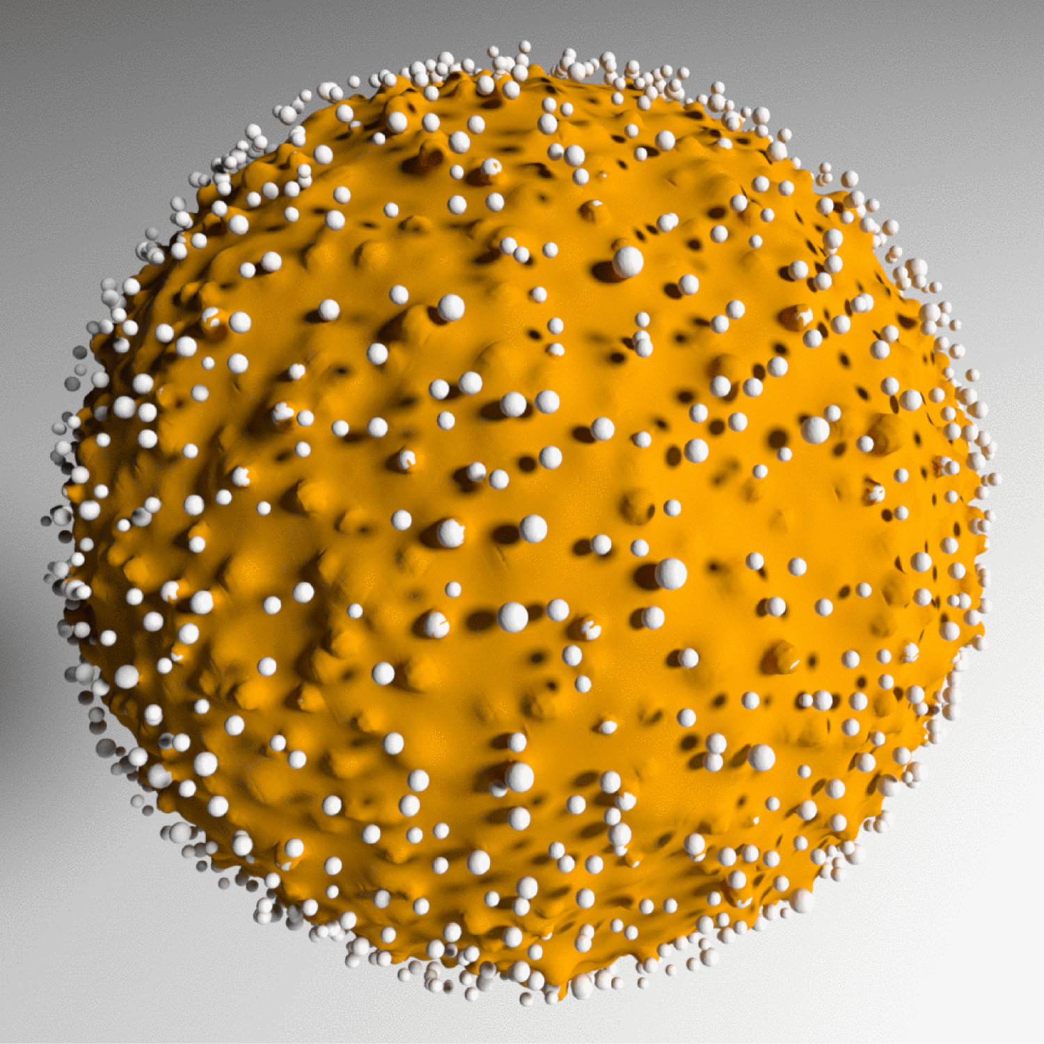
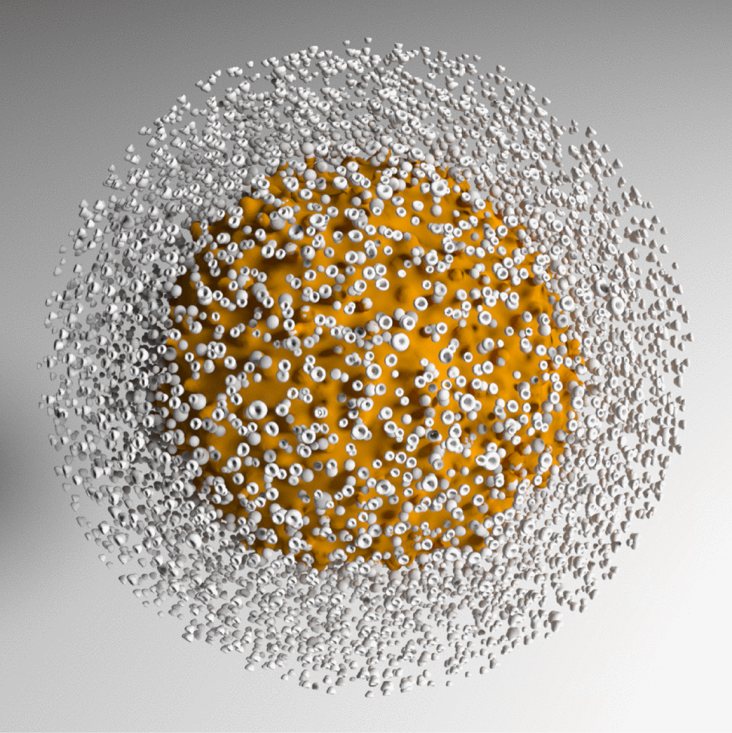
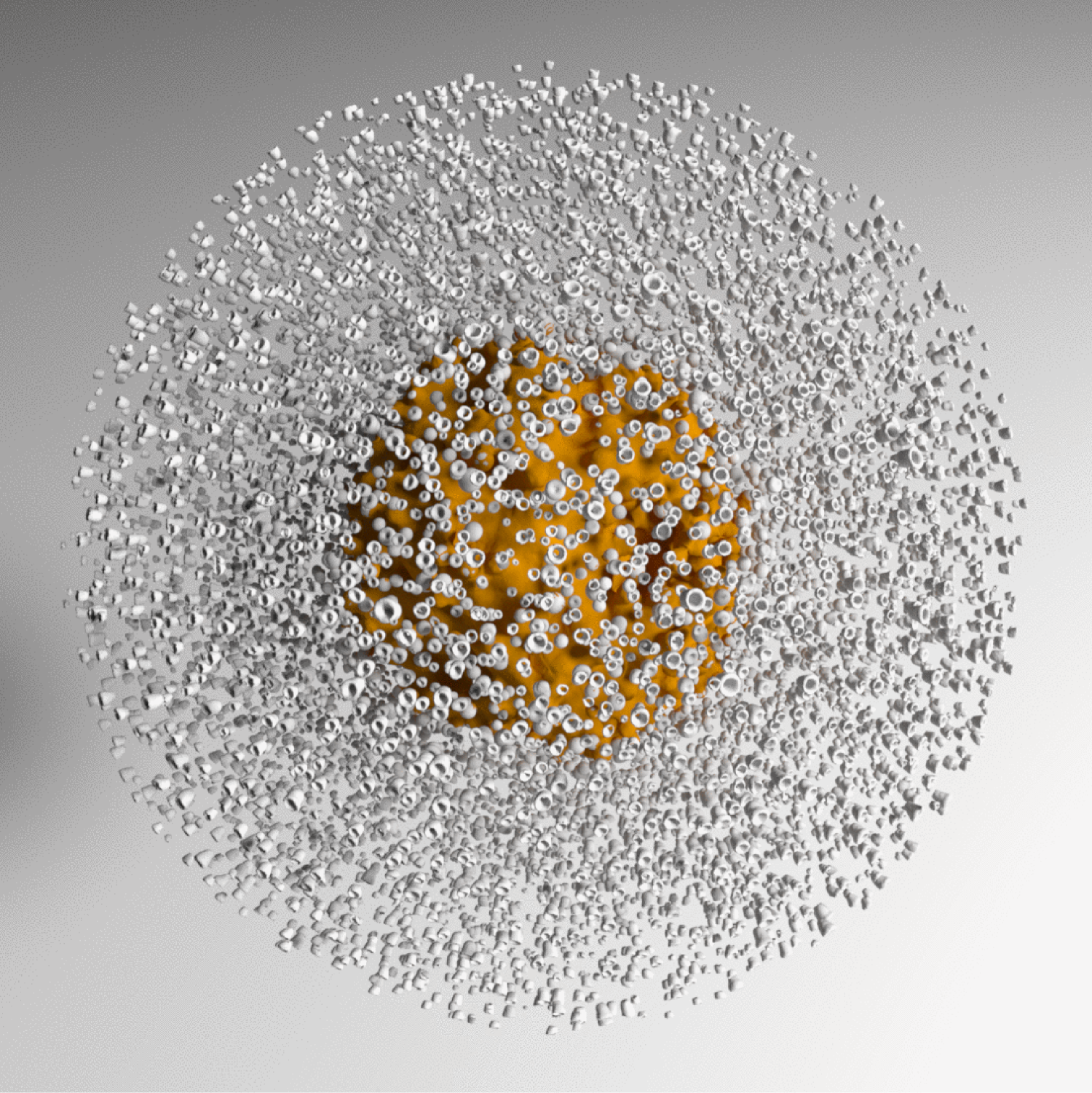
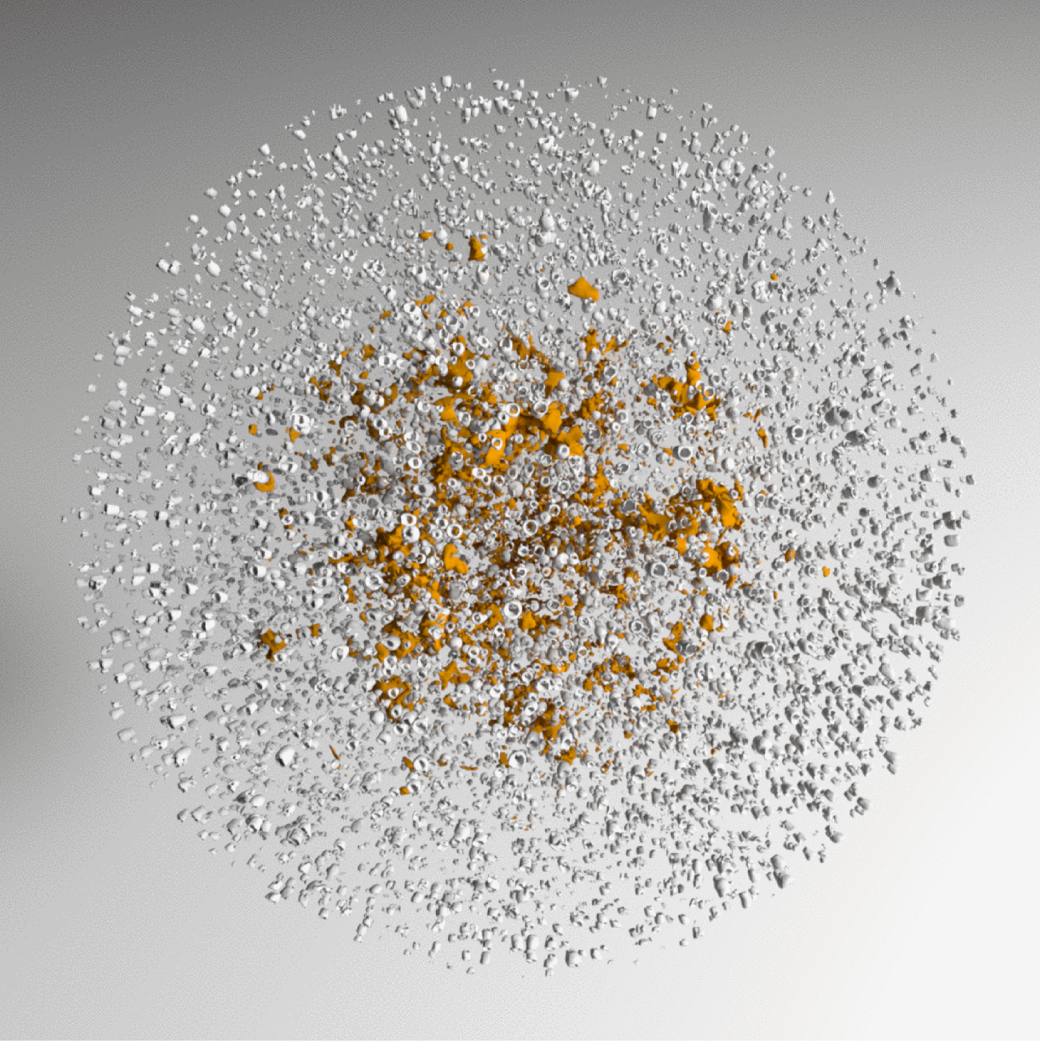
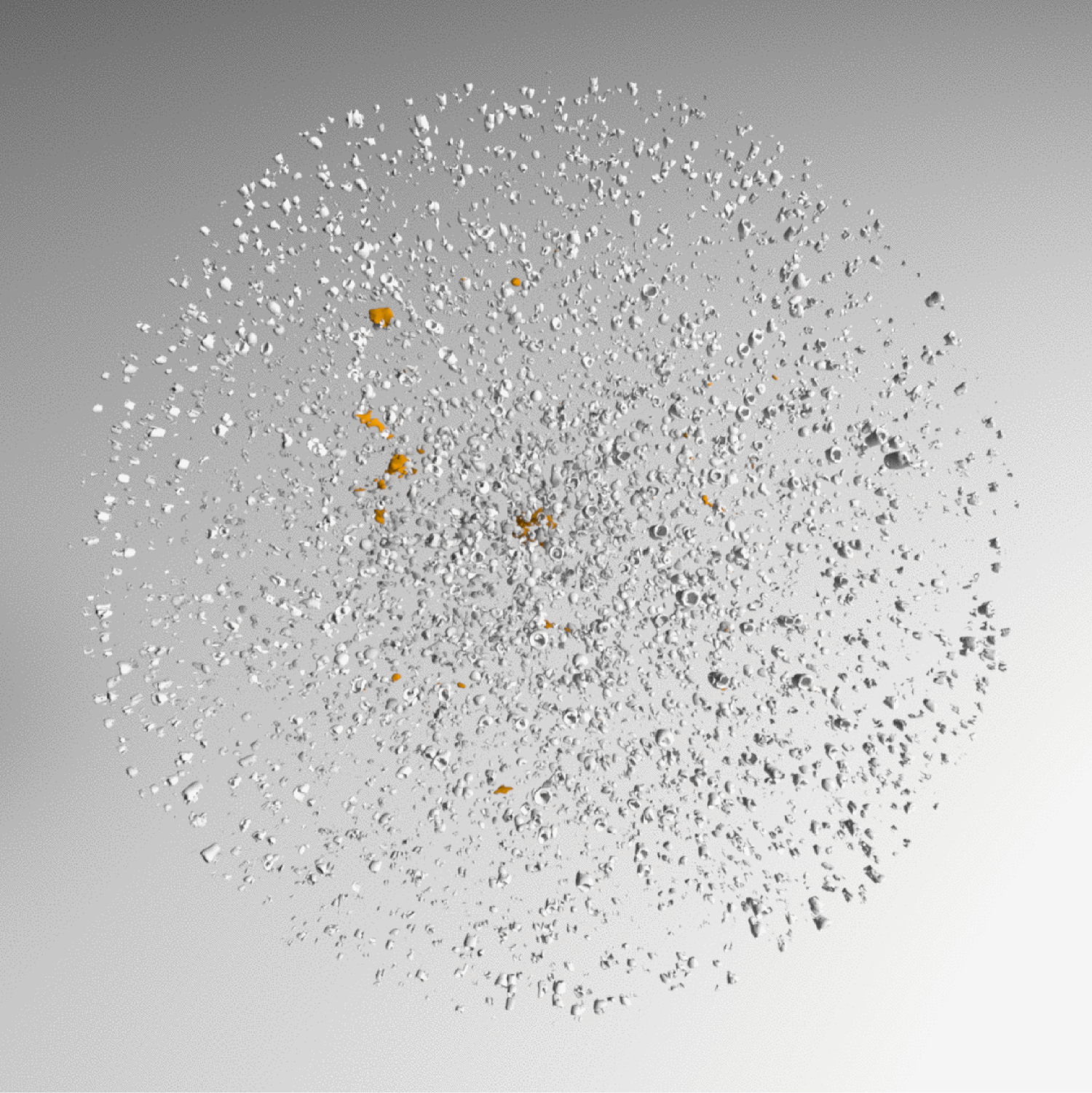
Figure 4: Temporal evolution of collapsing cloud with pressure iso-surface at $p_{\text{iso}}=0.15\>\mathrm{MPa}$.

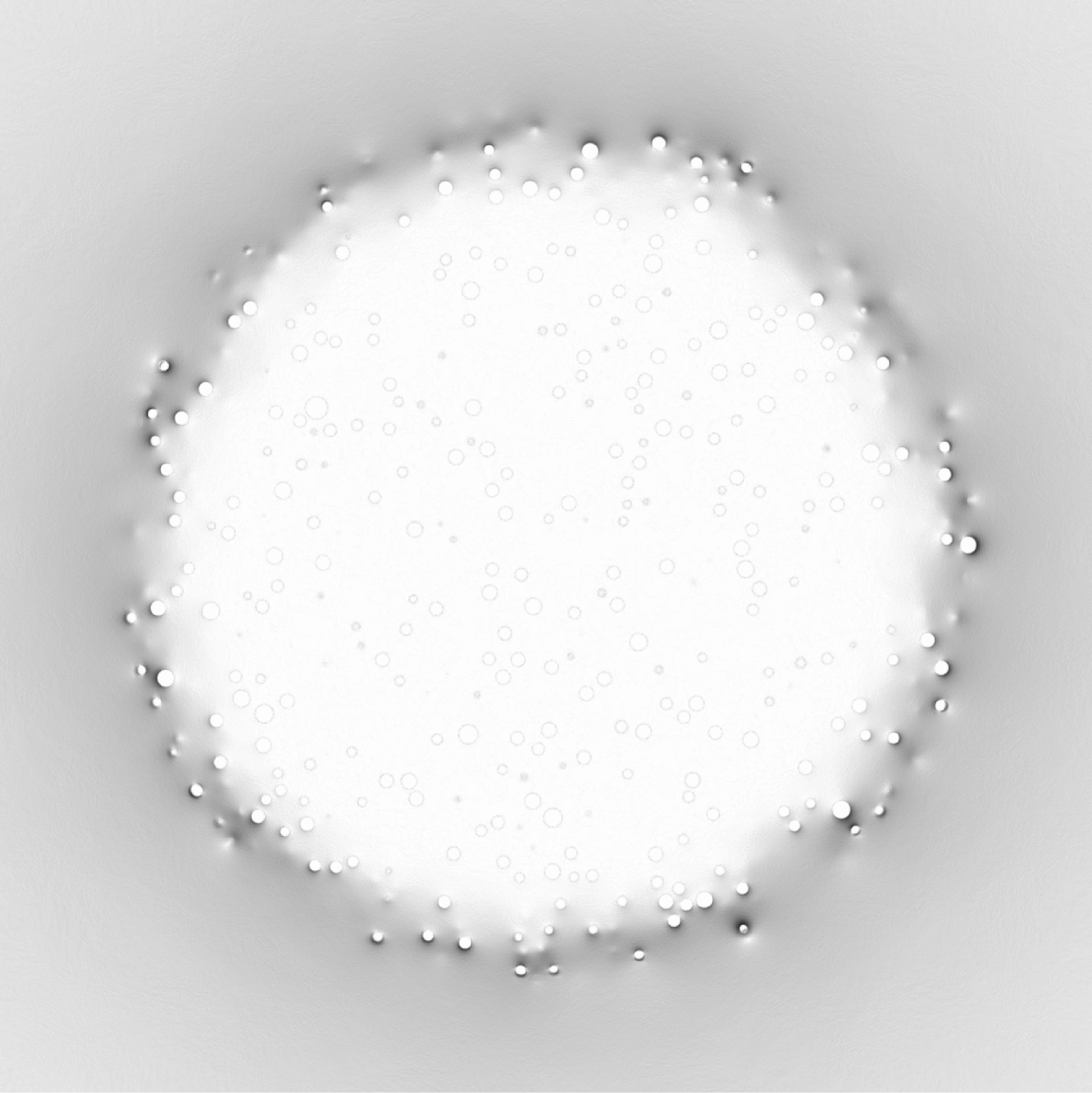
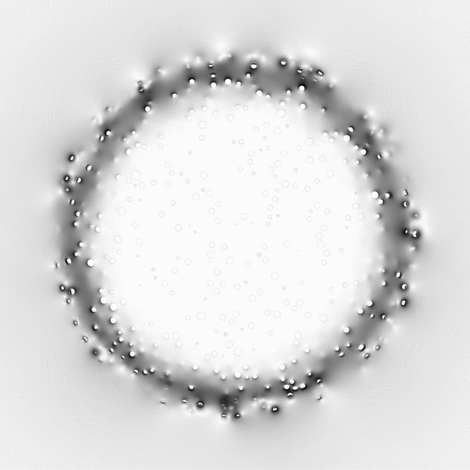
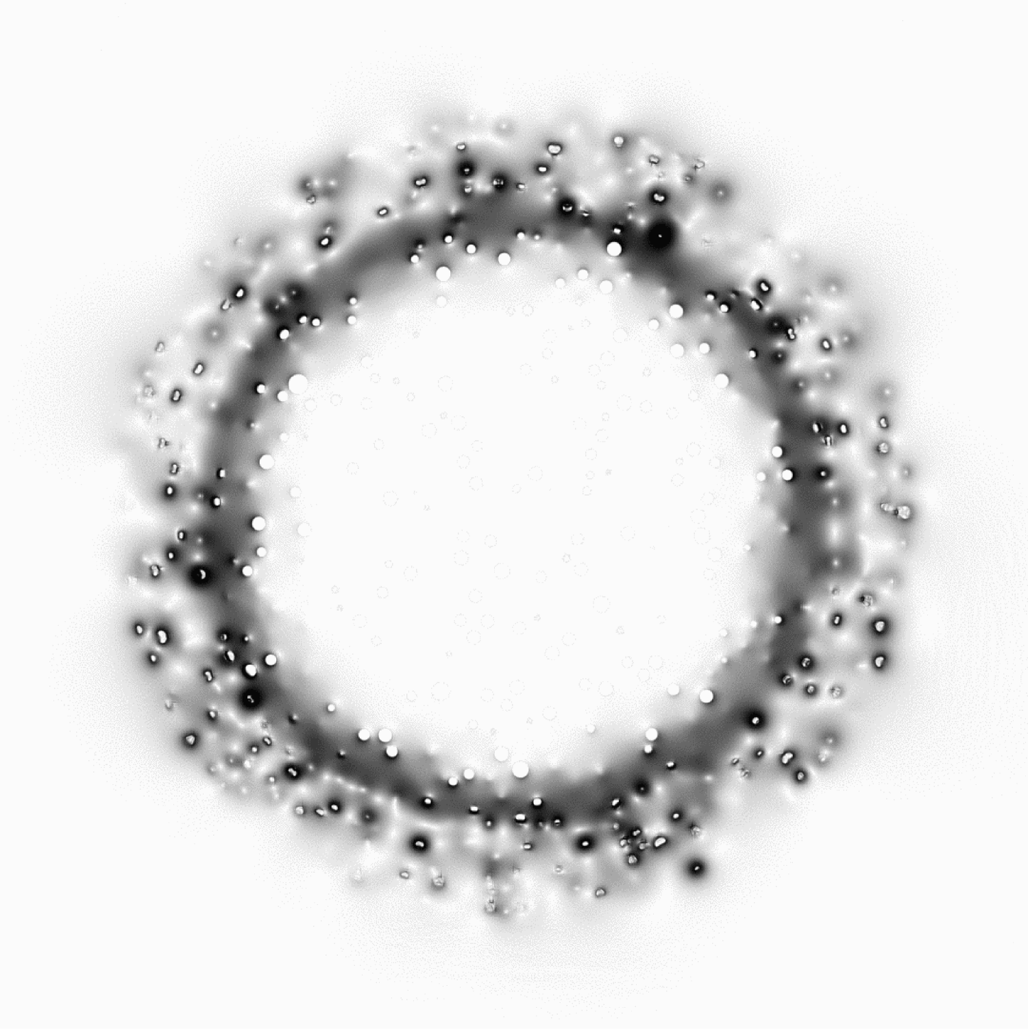
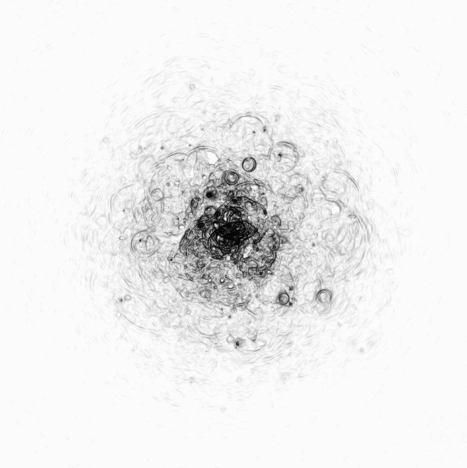
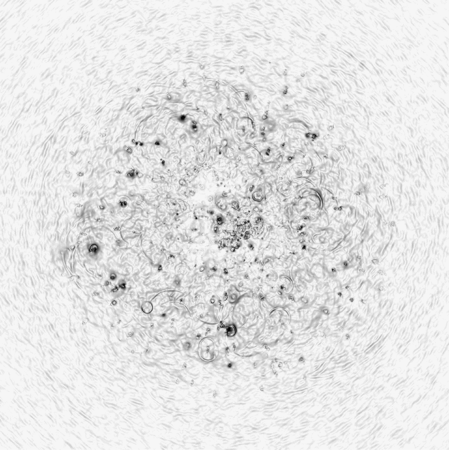
Figure 5: Temporal evolution of collapsing cloud visualized using numerical schlieren images of the pressure field in the $xy$-plane at $z=0$.

The minimum gas volume is reached at time $t_{\mathrm{C}}=343.9\>\mathrm{\mu s}$, which is referred to as the cloud collapse time in the following. At this time, the gas volume is reduced by $88$% compared to its initial value. The point-wise maximum pressure $p_{\mathrm{max}}$ is a highly fluctuating quantity. Its peak $p_{\mathrm{peak}}=3.41\>\mathrm{GPa}$ is detected at time $t/t_{\mathrm{C}}=0.898$ and occurs before the minimum gas volume is encountered. A similar observation was made in Yamamoto:2016 . To capture the behavior in the core of the cloud, we center a spherical pressure sensor of radius $R_{\mathrm{S}}=1\>\mathrm{mm}$ at the center of the cloud. The sensor measures the average pressure $p_{\mathrm{S}}$ over its domain. The maximum value of $p_{\mathrm{S}}$ amounts to $p_{\mathrm{S,peak}}=89.5\>\mathrm{MPa}$ and is observed at time $t/t_{\mathrm{C}}=0.901$. The pressure curve of the sensor reveals the shielding effect dAgostino:1989 ; Brennen:2005 of the outer bubbles in the cloud. Although a broad time interval of high pressures is observed for $p_{\mathrm{max}}$, merely the major peak and one smaller peak are detected by the sensor. Strong pressure waves emitted away from the immediate surrounding of the sensor are absorbed by bubbles between the source of the pressure wave and the sensor by contributing to the compression of these bubbles. The maximum value of the average pressure within the cloud is $p_{\mathrm{C,peak}}=3.69\>\mathrm{MPa}$ and significantly smaller than $p_{\mathrm{S,peak}}$. Furthermore, it is encountered at a later time $t/t_{\mathrm{C}}=1.021$, which is almost exactly the time of minimum gas volume. The kinetic energy of the mixture in the cloud region increases until it reaches its peak value of $E_{\mathrm{kin,C,peak}}=3.69\>\mathrm{J}$ at $t/t_{\mathrm{C}}=0.800$, which is before the occurrence of $p_{\mathrm{peak}}$. At time $t_{\mathrm{C}}$, the kinetic energy is already reduced by $72$%.

Fig. 4 illustrates the deformation of the bubbles, which is caused by the formation of microjets. As the collapse of the cloud progresses, the extracted pressure iso-surface is moving inward. Accordingly, an evolving circular front is detected by the numerical schlieren of the pressure field shown in Fig. 5. Figs. 4 and 5 thus reveal an inward-propagating spherical collapse wave and the aforementioned shielding effect. While the bubbles behind the front are subject to a collapse process, bubbles ahead of the front remain at their initial state. From the fourth to the fifth frame, a break-down of the shielding effect is observed. Furthermore, strong spherical pressure waves emitted from individual bubble collapses are clearly visible in the fifth numerical schlieren frame.

III.2 Collapse wave propagation

The large number of bubbles in the cloud renders the macroscopic flow spherically symmetric and allows for analyzing the collapse wave observed in the previous section. Therefore, spherical averages $\bar{\alpha}_{2}(r,t)$, $\bar{p}(r,t)$ and $\bar{u}(r,t)$ of the gas volume fraction, the pressure and the velocity magnitude are computed over spheres with radius $r$ centered at the cloud center. The radial position of the collapse wave front is defined by the location of the maximum average velocity magnitude as

$$R_{\mathrm{F}}(t)=\operatorname*{arg\,max}_{r}\bar{u}(r,t).$$ (15)

Fig. 6 shows the front trajectory in the $r$-$t$-space on top of a contour plot of $\bar{\alpha}_{2}(r,t)$ as well as the evolution of the front speed $\dot{R}_{\mathrm{F}}$.

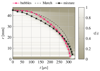
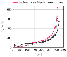
Figure 6: Front trajectory of collapse wave on $\bar{\alpha}_{2}$ contour plot (left) and front speed (right). Results obtained with the Mørch model and a homogeneous mixture approach are included for comparison.

Apart from these curves, labeled “bubbles”, predictions by simplified models which are further addressed below are also included. The propagation of the front starts immediately. The front gradually accelerates so that the front speed reaches $100\>\mathrm{m/s}$ at $t=150\>\mathrm{\mu s}$ and $200\>\mathrm{m/s}$ at $t=240\>\mathrm{\mu s}$. These velocities are lower than the speed of sound in both pure fluids which amounts to $1625\>\mathrm{m/s}$ for water and to $374\>\mathrm{m/s}$ for air under pressure $p_{\mathrm{C}}=0.1\>\mathrm{MPa}$. Eventually, the front reaches the speed of sound of air at approximately $t=270\>\mathrm{\mu s}$. At about the same time, the kinetic energy of the mixture in the cloud starts to decrease and pressure disturbances penetrate the front despite the shielding effect; see Fig. 3.

Profiles of the spherical averages at various time instants $t=139,183,218,245,267,285$ and $297\>\mathrm{\mu s}$ corresponding to $R_{\mathrm{F}}=40,35,30,25,20,15$ and $10\>\mathrm{mm}$ are shown in Fig. 7.

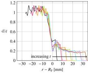
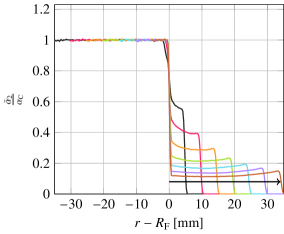
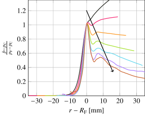
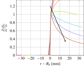
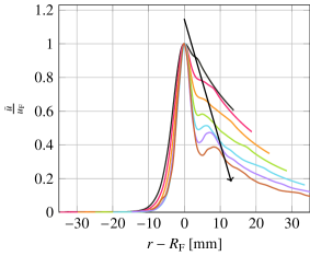
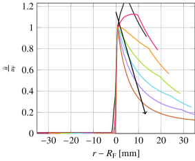
Figure 7: Normalized profiles of spherical averages of the gas volume fraction, pressure and velocity magnitude corresponding to $R_{\mathrm{F}}=40,35,30,25,20,15$ and $10\>\mathrm{mm}$. Simulation with resolved bubbles (left) and homogeneous mixture approach (right). Arrows indicate increasing time.

The profiles are normalized and plotted in the frame of reference of the front, i.e., depending on the relative radial location $r-R_{\mathrm{F}}(t)$. The normalized gas volume fraction, pressure and velocity are defined as ${\bar{\alpha}_{2}}/{\alpha_{\mathrm{C}}}$, $(\bar{p}-p_{\mathrm{C}})/(\bar{p}_{\mathrm{F}}-p_{\mathrm{C}})$ and ${\bar{u}}/{\bar{u}_{\mathrm{F}}}$, where $\bar{p}_{\mathrm{F}}(t)=\bar{p}(R_{\mathrm{F}}(t),t)$ and $\bar{u}_{\mathrm{F}}(t)=\bar{u}(R_{\mathrm{F}}(t),t)$ are pressure and velocity at the front. The gas volume fraction shows some oscillations which decay towards the cloud surface as more bubbles contribute to the averages with increasing $r$. The normalization of the radial profiles reveals their self-similarity in the vicinity of the front. The collapse wave, or bubbly shock, does not exhibit a sharp front, but has a finite thickness which is related to the dynamics of the individual collapsing bubbles (see Wijngaarden:1970 ; Ganesh:2016 and references therein). Consistent with the observations of the aforementioned studies, the thickness of the front is of the size of a few bubble length scales. From the velocity profiles in Fig. 7, we obtain a front thickness of approximately $10\>\mathrm{mm}$, which is about seven bubble diameters. Owing to the shielding effect by the outer bubbles, all fields remain at their initial values ahead of the front, i.e., for $r-R_{\mathrm{F}}<-10\>\mathrm{mm}$. Closer to the front, the gas volume fraction gradually decreases to $\alpha_{2}/\alpha_{\mathrm{C}}\approx 0.2$ at the front, while the pressure and the velocity grow towards their peak values. Behind the front, the gas volume fraction rebounds and reaches a value of $\alpha_{2}/\alpha_{\mathrm{C}}\approx 0.4$ at a distance of $r-R_{\mathrm{F}}\approx 3\>\mathrm{mm}$. The gas volume fraction rebound behind the front  Brennen:2005 is accompanied by a drop in the pressure and velocity. Farther outward from the cloud center, all profiles keep declining. At the cloud surface, the gas volume fraction drops to zero in a sharp fashion whereas pressure and velocity decrease smoothly to their prescribed far field values.

The values of the pressure and velocity at the front increase as seen from their temporal evolution shown in Fig. 8. As derived from mass and momentum balance Wijngaarden:1970 ; Morch:1989 , $p_{\mathrm{F}}$ and $u_{\mathrm{F}}$ are related to the front speed. Approximate relations for these quantities near the front are given by

$$p_{\mathrm{F}}-p_{\mathrm{C}} \sim\rho_{1}(1-\alpha_{\mathrm{C}})\alpha_{\mathrm{C}}\dot{R}_{\mathrm{F}}^{2},$$ (16)

$$u_{\mathrm{F}} \sim\alpha_{\mathrm{C}}\dot{R}_{\mathrm{F}}.$$ (17)

up to a scaling factor which depends on the definition of the front location. Fitting these relations to the simulation data results in

$$p_{\mathrm{F}}-p_{\mathrm{C}} =5.95\rho_{1}(1-\alpha_{\mathrm{C}})\alpha_{\mathrm{C}}\dot{R}_{\mathrm{F}}^{2},$$ (18)

$$u_{\mathrm{F}} =2.39\alpha_{\mathrm{C}}\dot{R}_{\mathrm{F}}$$ (19)

and provides a good approximation to the present results; see Fig. 8.

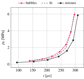
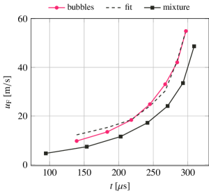
Figure 8: Temporal evolution of average pressure (left) and average velocity magnitude (right) at the front.

A model proposed by Mørch in Morch:1989 describes the collapse of a spherical cloud of vapor bubbles in the form of a Rayleigh-Plesset-like equation:

$$R_{\mathrm{F}}\ddot{R}_{\mathrm{F}}+\left(\frac{3}{2}-\frac{1}{2}(1-\psi)(1-\alpha_{\mathrm{C}})\right)\dot{R}_{\mathrm{F}}^{2}=-\frac{p_{\infty}-p_{v}}{\alpha_{\mathrm{C}}\rho_{1}},$$ (20)

where $p_{v}$ denotes the vapor pressure of the liquid and $\psi$ an energy conservation factor. The energy conservation factor accounts for energy losses due to the radiation of acoustic waves and dissipation. A larger value leads to a higher front speed. According to Morch:1989 , the energy conservation factor should be in the range $0\leq\psi\leq 0.5$. The model assumes that the bubbles are small compared to the cloud radius and that the vapor volume fraction is sufficiently high. In contrast to the present simulation of a cloud of gas bubbles, the Mørch model is derived for vapor bubbles which means that the pressure inside the bubbles remains constant during the collapse and that the bubbles collapse completely without any rebound stage. When setting $p_{v}=p_{\mathrm{C}}$, the Mørch model also provides a reasonable prediction for the front trajectory and speed of the present case, as can be seen from Fig. 6 where the respective curves are labeled “Mørch”. For the curves shown in Fig. 6, the energy conservation factor, which is only of minor influence, is set to $\psi=0.5$.

Furthermore, results obtained by a homogeneous mixture approach are included for comparison. The mathematical description introduced in Sec. II.1 may also be used to describe a homogeneous mixture of gas and liquid owing to the right-hand-side term of Eq. (5). Instead of initially prescribing a cloud composed of individual bubbles, a uniform gas volume fraction $\alpha_{2}=\alpha_{\mathrm{C}}$ is set within the sphere of radius $R_{\mathrm{C}}$. The initial conditions for the velocity and the pressure as well as the applied boundary conditions remain unchanged compared to the case with resolved bubbles. A similar approach was used in Tiwari:2015 . For the homogeneous mixture approach, the computational domain is discretized by $1024$ cells per spatial direction. Spherically averaged profiles for $R_{\mathrm{F}}=40,35,30,25,20,15$ and $10\>\mathrm{mm}$ corresponding to $t=94,154,203,242,271,293$ and $309\>\mathrm{\mu s}$, are shown in Fig. 7. In contrast to the case with resolved bubbles, the radial profiles are discontinuous at the front and do not demonstrate features such as the gas volume fraction rebound behind the front or the gradual transition of the profiles ahead of the front. Therefore, the location of the collapse wave front for the homogeneous mixture case is determined from the gas volume fraction via

$$R_{\mathrm{F}}(t)=\operatorname*{arg\,max}_{r}\left|\frac{\partial\bar{\alpha}_{2}}{\partial t}(r,t)\right|,$$ (21)

which detects the discontinuity in $\bar{\alpha}_{2}$. The front trajectory and speed, shown in Fig. 6 by the curves labeled “mixture”, are qualitatively similar to the ones of the resolved simulation. However, the front speed is underestimated starting from $t=150\>\mathrm{\mu s}$, and the deviation grows in time reaching about $50\>\mathrm{m/s}$ at $t=250\>\mathrm{\mu s}$. The temporal evolution of the pressure and the velocity at the front are included in Fig. 8. The values observed with the homogeneous mixture approach are about $30\%$ lower compared to the resolved simulation. In summary, our results indicate that the front trajectory and speed observed in the simulation with large numbers of bubbles are well captured by simplified models. The evolution of the pressure and the velocity near the front matches the theoretical relations and in turn validates the present numerical results.

IV Bubble dynamics

Next, the evolution of the bubbles in the cloud is examined. Their oscillation frequencies as well as the microjets leading to their deformation are investigated.

IV.1 Bubble oscillations

The shape of the bubbles is implicitly described by the gas-volume-fraction field $\alpha_{2}$, which is sampled at a frequency of $0.63\>\mathrm{MHz}$. The center $\mathbf{x}_{\mathrm{B}_{i}}(t)$ and the equivalent radius $R_{\mathrm{B}_{i}}(t)$ of bubble $i$ are calculated as

$$\mathbf{x}_{\mathrm{B}_{i}}(t) =\frac{1}{V_{\mathrm{B}_{i}}(t)}\int\limits_{\Omega_{\mathrm{B}_{i}}}\alpha_{2}\mathbf{x}\>\mathrm{d}V,$$ (22)

$$R_{\mathrm{B}_{i}}(t) =\left(\frac{3}{4\pi}V_{\mathrm{B}_{i}}(t)\right)^{1/3},$$ (23)

where

$$V_{\mathrm{B}_{i}}(t)=\int\limits_{\Omega_{\mathrm{B}_{i}}}\alpha_{2}\>\mathrm{d}V$$ (24)

is the bubble volume. The integration is performed over a spherical domain $\Omega_{\mathrm{B}_{i}}$ concentric with the bubble center of the previous time sample and with a radius equal to the initial bubble radius $R_{\mathrm{B}_{i}}(0)$. In order to improve the accuracy of peak detection, the function $R_{\mathrm{B}_{i}}(t)$ is interpolated in time with a cubic spline.

Fig. 9 shows the evolution of the equivalent bubble radius for a few bubbles selected at various radial locations. All curves are normalized by the initial bubble radius. A bubble starts to oscillate once it is overtaken by the collapse induced wave.

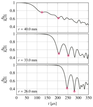
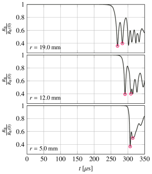
Figure 9: Temporal evolution of equivalent radius of selected bubbles at various radial locations $r=40.0,33.0,26.0,19.0,12.0$ and $5.0\>\mathrm{mm}$ (from top to bottom and left to right). Circles mark the minima for estimation of the oscillation frequency. All curves are normalized by the corresponding initial radius.

The oscillation frequency of each bubble in the cloud is calculated from the time between the first and second minimum of its equivalent radius, as marked in Fig. 9. A scatter plot of the bubble oscillation frequencies depending on the radial location is shown in Fig. 10 along with the moving average and the corresponding standard deviation computed with a window length of $4\>\mathrm{mm}$.

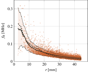
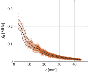
Figure 10: Scatter plot of bubble oscillation frequencies with respect to their radial location. Detailed simulation (left) and theoretical relation for a single bubble in an infinite liquid (right). Moving averages of the simulation data (solid line) and theoretical data (dashed line) are shown. Color shades indicate the standard deviation.

The oscillation frequency is higher for bubbles closer to the cloud center. The natural frequency of a single bubble oscillating in an unbounded liquid  Franc:2004 depends on the ambient pressure and the equilibrium radius of the bubble. Using $p_{{\mathrm{B}_{i}},\mathrm{F}}$, which is the average pressure $\bar{p}(r,t)$ at the front when it reaches bubble $i$, and the associated equilibrium radius obtained via

$$R_{{\mathrm{B}_{i}},\mathrm{F}}=R_{\mathrm{B}_{i}}(0)\left(\frac{p_{C}}{p_{{\mathrm{B}_{i}},\mathrm{F}}}\right)^{\frac{1}{3\gamma_{2}}},$$ (25)

the frequency of each bubble in the cloud is estimated as

$$f_{\mathrm{B}_{i}}=\frac{1}{2\pi R_{{\mathrm{B}_{i}},\mathrm{F}}}\sqrt{\frac{3\gamma_{2}p_{{\mathrm{B}_{i}},\mathrm{F}}}{\rho_{1}}}.$$ (26)

The resulting frequencies are likewise shown in Fig. 10. Although Eq. (26) does not account for the influence of the other bubbles in the cloud, this estimation is in a reasonable agreement with the simulation results. In particular, this result shows that the oscillation frequency of a bubble is governed by the front pressure and therefore, given Eq. (16), by the front speed.

IV.2 Microjet formation

The evolving pressure gradient along the bubble surface leads to the formation of a localized liquid jet of high velocity which notably deforms the bubble and eventually pierces though it. Following Jayaprakash:2012 , the tip $\mathbf{x}_{\mathrm{tip}_{i}}$ of the microjet associated with bubble $i$ is identified as the location of minimum curvature on the bubble surface. Here, the interface is represented by the iso-surface $\alpha_{2}=0.5$ of the gas-volume-fraction field. The curvature of any iso-contour of $\alpha_{2}$ can be calculated from the gas-volume-fraction field via $\kappa=-\nabla\cdot\frac{\nabla\alpha_{2}}{|\nabla\alpha_{2}|}$.

Fig. 11 illustrates the evolution of the microjet for three bubbles.

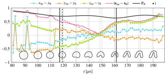
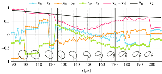
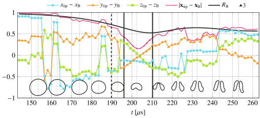
Figure 11: Temporal evolution of microjets for three selected bubbles. Trajectory of microjet tip relative to the bubble center (solid lines), linear fit (dashed lines) and equivalent radius (black solid line). All quantities are normalized by the corresponding initial radius. Fitting range $[t_{\mathrm{tip},i},t_{\mathrm{imp},i}]$ (vertical solid lines), collapse wave arrival $t_{\mathrm{F}}$ (vertical dashed line) and intervals of $10\>\mathrm{\mu s}$ with corresponding iso-lines of $\alpha_{2}=0.5$ at the bottom (vertical dotted lines).

The relative location of the tip, $\mathbf{x}_{\mathrm{tip},i}-\mathbf{x}_{\mathrm{B}_{i}}$, as well as the bubble radius $R_{\mathrm{B}_{i}}$ are displayed as a function of time. Additionally, bubble shapes are shown for selected time instants. At the beginning of the collapse process, the bubble surface is largely spherical and possesses a positive curvature. Therefore, the distance between the location of minimum curvature and the bubble center is approximately equal to the equivalent radius, but the location itself is not well-defined and thus bounces from one point to another. Once the microjet starts to form, the curvature changes its sign. The location of minimum curvature then identifies the tip of the microjet. The microjet deforms the bubble into a cap-like shape until it pierces through the bubble on the opposite surface; see Fig. 11. At this time, the distance between the location of minimum curvature and the bubble center again approximately equals the equivalent radius. Hence, the characteristic quantities of the microjets are evaluated during the time interval $[t_{\mathrm{tip},i},t_{\mathrm{imp},i}]$ for which

$$|\mathbf{x}_{\mathrm{B}_{i}}-\mathbf{x}_{\mathrm{tip},i}|<0.75R_{\mathrm{B}_{i}}$$ (27)

holds. As observed in Fig. 11, the relative trajectory $\mathbf{x}_{\mathrm{tip},i}-\mathbf{x}_{\mathrm{B}_{i}}$ of the tip of the microjet travels with approximately a constant velocity within this interval. The microjet velocity $\mathbf{u}_{\mathrm{tip},i}$ is defined by the time derivative of a linear fit of $\mathbf{x}_{\mathrm{tip},i}-\mathbf{x}_{\mathrm{B}_{i}}$ in the time interval $[t_{\mathrm{tip},i},t_{\mathrm{imp},i}]$. In order to obtain reliable statistics, the fitting range is required to comprise at least six samples in time (i.e., has duration of at least $10\>\mathrm{\mu s}$) and the root-mean-square error of the fitting has to be below $0.1\,R_{\mathrm{B}_{i}}(0)$. Due to the limited data sampling frequency and the complexity of the microjet tip trajectories, not all bubbles satisfy these requirements. Such bubbles are excluded from the subsequent analysis of the microjets, leaving about $7500$ bubbles (i.e., $60\%$ of the bubbles) for further evaluation.

As reported in preceding studies on cloud cavitation collapse Bremond:2006 ; Tiwari:2015 , the microjets point towards the core of the cloud. As shown in the present work, the axes of these microjets are not perfectly aligned with the radial direction $\mathbf{x}_{\mathrm{C}}-\mathbf{x}_{\mathrm{B}_{i}}(0)$ from the initial bubble center to the cloud center. The inclination angle $\theta_{i}$ denotes the angle between the radial direction and the direction of the microjet velocity corresponding to bubble $i$ as illustrated in Fig. 12.

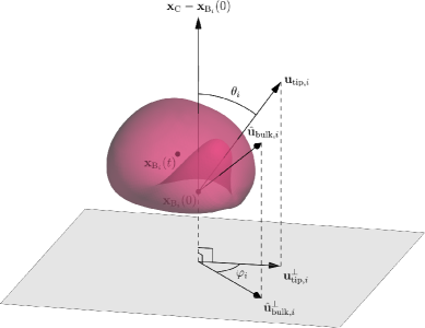
Figure 12: Bubble surface with microjet velocity $\mathbf{u}_{\mathrm{tip},i}$, bulk velocity indicator $\hat{\mathbf{u}}_{\mathrm{bulk},i}$ as well as their projections $\mathbf{u}^{\perp}_{\mathrm{tip},i}$ and $\hat{\mathbf{u}}^{\perp}_{\mathrm{bulk},i}$ onto a plane perpendicular to the radial direction.

A microjet with $\theta_{i}=0^{\circ}$ is directed towards the cloud center. Values of the inclination angle for bubbles shown in Fig. 11 are given in Table 1 where the microjet of bubble “2” is distinguished by stronger inclination. Fig. 13 depicts a scatter plot of the inclination angle $\theta_{i}$ versus the radial distance $r$.

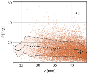
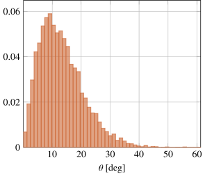
Figure 13: Microjet inclination angle $\theta_{i}$ depending on radial location (left) and PDF of the inclination angle (right).

All scatter plots shown in this subsection also contain the moving average and the standard deviation computed with a window length equal to $10\%$ of the corresponding horizontal axis range. The bubbles selected in Fig. 11 are also marked. Furthermore, Fig. 13 depicts the Probability Density Function (PDF) of the inclination angle. The average inclination angle for the present cloud collapse process is $13.2^{\circ}$. Furthermore, $90\%$ of the bubbles exhibit an inclination angle smaller than $24^{\circ}$. Local mean values of the inclination angle range from $10^{\circ}$ at $r=45\>\mathrm{mm}$ to $18^{\circ}$ at $r=26\>\mathrm{mm}$. As a result, the microjet inclination angle increases slightly towards the cloud center indicating a weak dependence on the collapse wave speed, which strongly depends on $r$. Very large inclination angles in the range of $35^{\circ}$ to $61^{\circ}$ are observed for $1\%$ of the bubbles. Closer examination of these microjets reveals that the microjet inclination is affected by the surrounding bubbles. Fig. 15 shows the neighborhood of a bubble with an inclination angle of $50^{\circ}$.

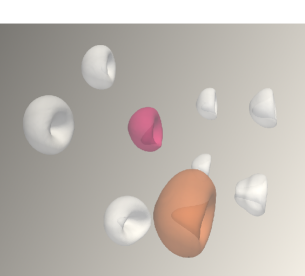
Figure 14: Neighborhood of a small bubble (red) with a large inclination angle of $50^{\circ}$ that is attracted towards a significantly larger bubble nearby (brown).

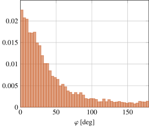
Figure 15: PDF of angle $\varphi_{i}$ between $\mathbf{u}^{\perp}_{\mathrm{tip},i}$ and $\hat{\mathbf{u}}^{\perp}_{\mathrm{bulk},i}$.

The microjet is inclined towards one specific neighboring bubble that has a significantly larger size than the considered bubble as well as all the other bubbles in its vicinity. This observation suggests that the microjet inclination mainly depends on the geometrical arrangement of the bubbles. Larger bubbles have a stronger influence on the liquid flow. Assuming potential flow away from the bubbles, the velocity in the surrounding liquid is given by  Mettin:1997 :

$$\mathbf{u}(\mathbf{x},t)=\sum\limits_{j=1}^{n_{B}}\frac{R_{\mathrm{B}_{j}}^{2}\dot{R}_{\mathrm{B}_{j}}}{|\mathbf{x}-\mathbf{x}_{\mathrm{B}_{j}}|^{3}}(\mathbf{x}-\mathbf{x}_{\mathrm{B}_{j}}).$$ (28)

Furthermore, the bubble compression rate $\dot{R}_{\mathrm{B}_{j}}$ in Eq. (28) is taken to be constant and negative leading to a non-dimensional bulk velocity

$$\hat{\mathbf{u}}_{\mathrm{bulk},i}=\sum\limits_{\begin{subarray}{c}j=1\\ j\neq i\end{subarray}}^{n_{B}}\frac{-R_{\mathrm{B}_{j}}^{2}(0)}{|\mathbf{x}_{\mathrm{B}_{i}}(0)-\mathbf{x}_{\mathrm{B}_{j}}(0)|^{3}}(\mathbf{x}_{\mathrm{B}_{i}}(0)-\mathbf{x}_{\mathrm{B}_{j}}(0))$$ (29)

at the center $\mathbf{x}_{\mathrm{B}_{i}}$ of bubble $i$. Eq. (29) provides an estimation for the bulk flow direction and its strength which is purely based on the initial geometrical arrangement. The assumption of constant $\dot{R}_{\mathrm{B}_{j}}$ does not exactly hold for cloud collapses since the bubbles behind the collapse front compress but remain at rest ahead of it. Therefore, Eq. (29) characterizes only the flow velocity perpendicular to the radial direction which is governed by the arrangement of bubbles along the collapse front. To examine the influence of the bulk flow induced by the collapse of the surrounding bubbles on the microjet direction, $\mathbf{u}_{\mathrm{tip},i}$ and $\hat{\mathbf{u}}_{\mathrm{bulk},i}$ are projected onto a plane perpendicular to the radial direction. The resulting velocity components are marked by the additional superscript $(\cdot)^{\perp}$ and are also schematically represented in Fig. 12. The angle between $\mathbf{u}^{\perp}_{\mathrm{tip},i}$ and $\hat{\mathbf{u}}^{\perp}_{\mathrm{bulk},i}$ is denoted $\varphi_{i}$. The PDF of $\varphi_{i}$ as well as scatter plots of $\varphi_{i}$ versus $\theta_{i}$ and $\theta_{i}$ versus the magnitude $|\hat{\mathbf{u}}^{\perp}_{\mathrm{bulk},i}|$ of the projected bulk velocity are shown in Figs. 15 and 16, respectively. For $68\%$ of the bubbles, $\varphi_{i}$ is smaller than $45^{\circ}$, which demonstrates that the microjets are inclined towards the direction of the bulk liquid flow around the bubble. This angle reduces with increasing inclination. The mean value of $\varphi_{i}$ is $45^{\circ}$ for $\theta_{i}=10^{\circ}$ and $25^{\circ}$ for $\theta_{i}=40^{\circ}$. Moreover, a positive correlation between the inclination angle $\theta_{i}$ and the magnitude of the projected component of the bulk flow indicator $|\hat{\mathbf{u}}^{\perp}_{\mathrm{bulk},i}|$ is observed.

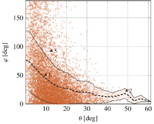
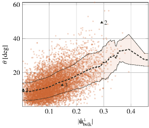
Figure 16: Angle $\varphi_{i}$ between $\mathbf{u}^{\perp}_{\mathrm{tip},i}$ and $\hat{\mathbf{u}}^{\perp}_{\mathrm{bulk},i}$ depending on inclination angle $\theta_{i}$ (left) and inclination angle depending on the magnitude $|\hat{\mathbf{u}}^{\perp}_{\mathrm{bulk},i}|$ (right).

Fig. 17 displays scatter plots of the microjet velocity magnitude depending on various quantities.

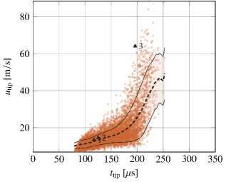
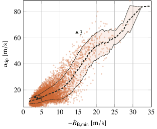
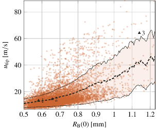
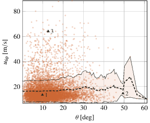
Figure 17: Microjet tip velocity depending on microjet initiation time $t_{\mathrm{tip},i}$, bubble compression rate $-\dot{R}_{\mathrm{B}_{i},\mathrm{min}}$, bubble initial radius $R_{\mathrm{B}_{i}}(0)$ and inclination angle $\theta_{i}$ (from left to right and top to bottom).

The velocity magnitude of the microjets increases with their time of initiation. For instance, the mean value amounts to $10\>\mathrm{m/s}$ for $t_{\mathrm{tip}}=80\>\mathrm{\mu s}$ and to $50\>\mathrm{m/s}$ for $t_{\mathrm{tip}}=250\>\mathrm{\mu s}$. This behavior is consistent with the acceleration of the cavitation collapse wave and the growth of the pressure at the front. One of the fastest microjets is observed for bubble “3” included in Fig. 11 and Table 1. The scatter plot of the microjet velocity magnitude versus the initial bubble radius $R_{B}(0)$ shows that larger bubbles exhibit faster microjets. The mean value rises from $20$ to $40\>\mathrm{m/s}$ for bubbles with an initial radius between $0.5$ and $1.2\>\mathrm{mm}$. Another quantity relevant to the collapse strength of a bubble is the peak compression rate $-\dot{R}_{\mathrm{B}_{i},\min}$ which is evaluated within the time interval $[t_{\mathrm{tip},i},t_{\mathrm{imp},i}]$. A positive correlation of the compression rate with the magnitude of the microjet velocity is observed in Fig. 17. In contrast, the inclination angle $\theta_{i}$ does not affect the magnitude of the microjet velocity. The analyzed relations reveal that the microjet velocity is influenced by both parameters of individual bubbles (e.g., the initial bubble radius) and macroscopic parameters of the cloud collapse (e.g., the collapse front speed). However, the overall large dispersion of these relations indicates the influence of further factors such as the spatial configuration of the surrounding bubbles.

Table 1: Microjet parameters of selected bubbles.

bubble	$r\>\mathrm{[mm]}$	$\theta\>\mathrm{[deg]}$	$u_{\mathrm{tip}}\>\mathrm{[m/s]}$	$R_{\mathrm{B}}(0)\>\mathrm{[mm]}$	$-\dot{R}_{\mathrm{B},\min}\>\mathrm{[m/s]}$	$\varphi\>\mathrm{[deg]}$	$|\hat{\mathbf{u}}^{\perp}_{\mathrm{bulk}}|$
1	41.9	9.8	13.4	0.58	3.9	50.6	0.005
2	41.4	49.4	14.6	0.66	3.3	22.9	0.293
3	34.1	12.6	64.1	1.14	14.7	92.5	0.148

V Pressure pulse spectrum

While the propagation of the collapse wave through the cloud may also be well recovered by analytically simplified relations and homogeneous mixture approaches as shown in Sec. III.2, predictions regarding the hydrodynamic aggressiveness of cloud cavitation collapse require capturing the pressure pulses generated by individual bubble collapses  Kim:2014 . The pressure pulse spectrum describes the rate and strength of collapse-induced pressure pulses and may also be used to assess the erosive potential in case of wall-bounded cavitating flow. If the pressure pulses are continuously emitted close to a material surface, the resulting repeated loading acting on the surface causes failure of the material and mass loss. To experimentally capture collapse-induced pressure loads, high frequency pressure sensors placed at predefined locations are frequently used Franc:2011b ; Singh:2013 . Alternatively, they are recovered from pitting tests with ductile materials  Jayaprakash:2012b ; Franc:2012a . In contrast to experiments, numerical simulations provide spatially and temporally resolved information, enabling a more comprehensive picture.

V.1 Identification of pressure pules

We evaluate the pressure pulse spectrum by identifying individual pressure pulses encountered in the center plane, i.e., the $xy$-plane at $z=0$, of the cloud. This identification involves the following steps:

• Each grid cell of the center plane serves as a pressure sensor whose sampling frequency is $2.53\>\mathrm{MHz}$, as illustrated in Fig. 18. Data is collected up to the collapse time of the cloud, i.e., the time of minimum gas volume.

• For each cell, all pressure peaks are collected that are above a threshold pressure $p_{\mathrm{th}}=20\>\mathrm{MPa}$; see also Fig. 18. If several peaks are detected for a time interval with $p>p_{\mathrm{th}}$, only the highest peak value is kept, as also done for experimentally measured pressure signals Singh:2013 .

• At each sampling time, all cells exhibiting a peak pressure above $p_{\mathrm{th}}$ are considered as potential locations of a pressure pulse.

• For a given sampling time, neighboring cells with a peak pressure above $p_{\mathrm{th}}$ are grouped together to form the footprint of a single pressure pulse acting at this time. The number of cells contributing to the footprint is denoted by $n_{cf}$.

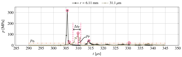
Figure 18: Pressure signal at two cells located at $r=6.11\>\mathrm{mm}$ and $31.1\>\mathrm{\mu m}$. Collected pressure peaks are marked by circles. The threshold pressure is indicated by a horizontal line. Characteristic quantities of a pressure pulse are illustrated.

The center $\mathbf{x}_{\mathrm{P}}$ of the footprint of a pulse detected at time $t_{\mathrm{P}}$ is given by the location of the cell $n_{i}$ with the highest peak pressure value $p_{\mathrm{P}}=\max{p_{n_{i}}}$, where $i\in{1,...,n_{cf}}$. The extent of the footprint is defined as the equivalent diameter of the area covered by the $n_{cf}$ combined cells, i.e., $d_{\mathrm{P}}=2h\sqrt{n_{cf}/\pi}$. The duration $\Delta t_{\mathrm{P}}$ of the action of the pulse is given by the time period with $p>p_{\mathrm{th}}$ at the cell with pressure $p_{\mathrm{P}}$; see also Fig. 18.

Fig. 20 visualizes the pressure pulses detected in the center plane during the collapse of the cloud. Each pressure pulse is represented by a circle with diameter $d_{\mathrm{P}}$ centered at $\mathbf{x}_{\mathrm{P}}$ and colored by $p_{\mathrm{P}}$.

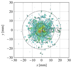
Figure 19: Pressure pulses visualized by colored circles with diameter $d_{\mathrm{P}}$. Blue color corresponds to pressure values close to the threshold pressure and red color to highest pressures.

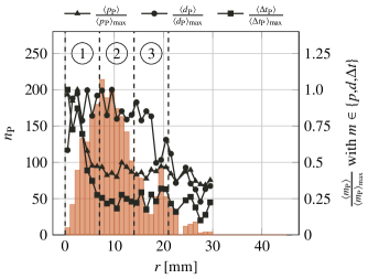
Figure 20: Histogram of pressure pulse distribution versus the distance from the center of the cloud and normalized average values for the peak pressure $\langle p_{\mathrm{P}}\rangle$, diameter $\langle d_{\mathrm{P}}\rangle$ and duration $\langle\Delta t_{\mathrm{P}}\rangle$.

The highest pressure in pulses is observed close to the center of the cloud. The histogram in Fig. 20 shows the number of pressure pulses depending on the radial distance along with the corresponding average values $\langle d_{\mathrm{P}}\rangle$, $\langle p_{\mathrm{P}}\rangle$ and $\langle\Delta t_{\mathrm{P}}\rangle$. All average quantities are normalized by their maximum values, which are $\langle d_{\mathrm{P}}\rangle_{\mathrm{max}}=0.69\>\mathrm{mm}$, $\langle p_{\mathrm{P}}\rangle_{\mathrm{max}}=67.06\>\mathrm{MPa}$ and $\langle\Delta t_{\mathrm{P}}\rangle_{\mathrm{max}}=1.63\>\mathrm{\mu s}$, respectively. The average diameter remains approximately constant up to a radial distance of $r=17\>\mathrm{mm}$ and then rapidly decreases. As also indicated by Fig. 20, the pressure achieves its highest value near the center, decreases as long as $r<7\>\mathrm{mm}$ and continues without changing significantly. A similar behavior is observed for the average pulse duration. The number of pulses quickly increases from the center reaching its maximum close to $r=7\>\mathrm{mm}$ and declines afterwards. Therefore, the center region is exposed to few but strong pressure pulses whereas the majority of weaker pulses occurs away from the center.

V.2 Pressure pulse rate

A collapsing cloud of bubbles causes a rich distribution of pressure pulses. For further analysis, the center region, where almost all pulses are encountered, is divided into three circular rings of equal thickness $\Delta r=7\>\mathrm{mm}$ as illustrated in Figs. 20 and 20. As seen in Fig. 20, the center-most ring $1$ contains the strongest and widest pressure pulses, ring $2$ in the middle summarizes the first part of the plateau region into which most of the pulses fall, and the outer-most ring $3$ is determined by the second part of the plateau region where the pulses are only very loosely packed.

The detected pressure pulses in each ring $1$ to $3$ can be classified according to their peak pressure, the diameter of their footprints and the duration of their action. The results are presented in the form of cumulative histograms of the pressure pulse rate as a function of the aforementioned quantities. The cumulative pressure pulse rate $\dot{N}_{\mathrm{P}}$ is defined as the number of pulses per unit time and unit area whose peak pressure, footprint or duration exceeds a given threshold value. The cumulative pressure pulse rate of the simulation is obtained by dividing the number of pressure pulses, counted based on the criterion given above, by the exposure time and the area of the region of interest. The exposure time is equal to the collapse time of the cloud, i.e., the complete sampling period. The region of interest is given by the area of the circular ring for which $\dot{N}_{\mathrm{P}}$ is evaluated.

Fig. 21 displays the cumulative pressure pulse rate versus the peak pressure $p_{\mathrm{P}}$, the diameter $d_{\mathrm{P}}$ and the duration $\Delta t_{\mathrm{P}}$. Data from all three rings are included.

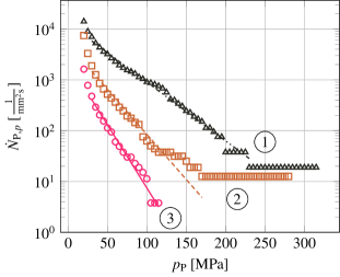
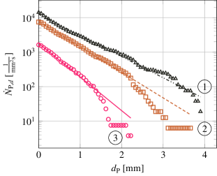
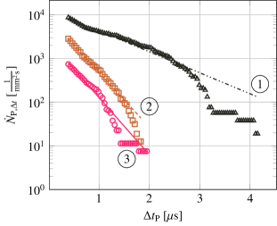
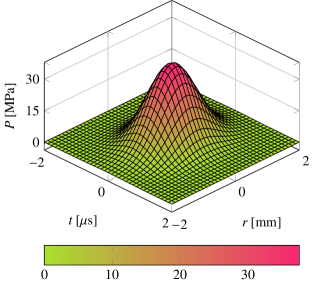
Figure 21: Cumulative histograms of pressure pulse rate versus peak pressure $p_{\mathrm{P}}$, diameter $d_{\mathrm{P}}$ and duration $\Delta t_{\mathrm{P}}$ for all rings as well as representative pressure pulse $P$ for the center-most ring $1$ (from left to right and top to bottom). Symbols correspond to simulation data and lines to fitted curves.

It has been suggested in Franc:2011b ; Singh:2013 ; Jayaprakash:2012b that the cumulative pressure pulse rate can be approximated by an exponential function of the form

$$\dot{N}_{\mathrm{P},m}=\dot{N}_{\mathrm{P},m}^{*}\mathrm{e}^{-\frac{m_{\mathrm{P}}}{m_{\mathrm{P}}^{*}}},$$ (30)

where $m\in\{p,d,\Delta t\}$. Exponent $-m_{\mathrm{P}}/m_{\mathrm{P}}^{*}$ may be additionally enhanced by a shape factor $\ell$ leading to $-(m_{\mathrm{P}}/m_{\mathrm{P}}^{*})^{\ell}$ Jayaprakash:2012b ; Singh:2013 . As done in Franc:2011b , a simple exponential law (i.e., $\ell=1$) is applied since it already provides appropriate approximations to our data. The two parameters $\dot{N}_{\mathrm{P},m}^{*}$ and $m_{\mathrm{P}}^{*}$ are a reference cumulative pressure pulse rate and a reference pressure, diameter or duration, respectively, that characterize the hydrodynamic aggressiveness of the collapsing cloud. To fit Eq. (30), which is of exponential form $y=a\mathrm{e}^{bx}$, to the data, a least squares method minimizing the residual $\sum y_{i}(\ln y_{i}-a-bx_{i})^{2}$ is used. The fitted curves are also included in Fig. 21, and the corresponding values for $\dot{N}_{\mathrm{P},m}^{*}$ and $m_{\mathrm{P}}^{*}$ are provided in Tab. 2.

Table 2: Regression parameters of the exponential function for the cumulative pressure pulse rate.

ring	$\dot{N}_{\mathrm{P},p}^{*}\>\mathrm{[1/(mm^{2}s)]}$	$p_{\mathrm{P}}^{*}\>\mathrm{[MPa]}$	$\dot{N}_{\mathrm{P},d}^{*}\>\mathrm{[1/(mm^{2}s)]}$	$d_{\mathrm{P}}^{*}\>\mathrm{[mm]}$	$\dot{N}_{\mathrm{P},\Delta t}^{*}\>\mathrm{[1/(mm^{2}s)]}$	$\Delta t_{\mathrm{P}}^{*}\>\mathrm{[\mu s]}$
$1$	$12968$	$37.56$	$12551$	$0.71$	$12958$	$0.90$
$2$	$4996$	$24.51$	$7750$	$0.59$	$8729$	$0.35$
$3$	$2280$	$17.48$	$1794$	$0.45$	$2596$	$0.33$

All data sets are well captured by the exponential law for the smaller values of $m_{\mathrm{P}}$. Both $\dot{N}_{\mathrm{P},m}^{*}$ and $m_{\mathrm{P}}^{*}$ decrease from the center-most ring $1$ to the outer-most ring $3$. The present results for $d_{\mathrm{P}}$ and $p_{\mathrm{P}}$ compare well to the respective diagrams from other cavitation problems provided in Franc:2012a (see Fig. $5$ therein for the diameter) and Mihatsch:2015 (see Fig. $15$ therein for the pressure). Those diagrams also recover the exponential law for the smaller values of $m_{\mathrm{P}}$ and reveal some deviations for larger values. In particular, larger values of $m_{\mathrm{P}}$ correspond to rare events which are not fully captured by only one collapse process. Furthermore, a maximum diameter has to be expected according to Kim:2014 for $d_{\mathrm{P}}$ which explains the fast decrease of $\dot{N}_{\mathrm{P},d}$ for larger values. A similar fast decay is observed for $\dot{N}_{\mathrm{P},\Delta t}$ here.

The values for $p_{\mathrm{P}}^{*}$, $d_{\mathrm{P}}^{*}$ and $\Delta t_{\mathrm{P}}^{*}$ allow for recovering a representative pressure pulse $P$ for the present cloud collapse process. Following Singh:2013 ; Choi2014 , the encountered impact loads caused by the collapse of cavitation bubbles can be approximated by a Gaussian function in space and time as

$$P=p_{\mathrm{P}}^{*}\mathrm{e}^{-\left(\frac{t}{\Delta t_{\mathrm{P}}^{*}}\right)^{2}}\mathrm{e}^{-\left(\frac{r}{d_{\mathrm{P}}^{*}}\right)^{2}}.$$ (31)

In Singh:2013 , the characteristic pressure and duration of Eq. (31) were estimated by using a linear curve fitted to the peak pressure versus the duration for a Gaussian function in time only. Exemplarily, Fig. 21 displays the representative impact load of ring $1$.

V.3 Coverage rate

Using $\dot{N}_{\mathrm{P},d}^{*}=8/(\pi\delta^{2}\tau)$ and $d_{\mathrm{P}}^{*}=\delta/2$, Eq. (30) may be rewritten as

$$\dot{N}_{\mathrm{P}}=\frac{8}{\pi\delta^{2}\tau}\mathrm{e}^{-\frac{2d_{\mathrm{P}}}{\delta}},$$ (32)

see Franc:2012a . The values of the two parameters $\delta$ and $\tau$ are calculated from $\dot{N}_{\mathrm{P},d}^{*}$ and $d_{\mathrm{P}}^{*}$ and are provided in Tab. 3.

Table 3: Characteristic parameters of the coverage rate.

ring	$\delta\>\mathrm{[mm]}$	$\tau\>\mathrm{[ms]}$
$1$	$1.42$	$0.10$
$2$	$1.18$	$0.24$
$3$	$0.89$	$1.79$

Parameter $\delta$ is a characteristic diameter of the footprint and parameter $\tau$ a characteristic time. Both parameters are related to the cumulative coverage rate $\beta$ which is given by

$$\beta=\frac{1}{\tau}\left(1+\frac{2d_{\mathrm{P}}}{\delta}+\frac{2d_{\mathrm{P}}^{2}}{\delta^{2}}\right)\mathrm{e}^{-\frac{2d_{\mathrm{P}}}{\delta}}$$ (33)

and derived in Franc:2012a . The cumulative coverage rate $\beta$ is interpreted as the fraction of the center plane that encounters pressure pulses with a footprint larger than a given $d_{\mathrm{P}}$. When $d_{\mathrm{P}}$ approaches zero, $\beta$ goes to $1/\tau$. Hence, $\tau$ denotes the coverage time and represents the time required to fully cover the center plane by pressure pulses. Fig. 22 displays the cumulative coverage rate obtained from the simulation together with the curves obtained from Eq. (33) by inserting the values for $\delta$ and $\tau$ given in Tab. 3. The cumulative coverage rate of the simulation is determined by, first, summing up the area of all impacts that exhibit a footprint with a diameter larger than a specified threshold value and, second, dividing by the exposure time and the area of the region of interest, as done for $\dot{N}_{\mathrm{P}}$.

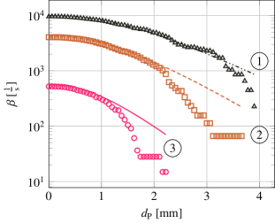
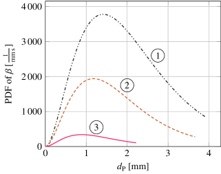
Figure 22: Cumulative histogram of coverage rate (left) and its estimated PDF (right). Symbols correspond to simulation data and lines to fitted curves.

The PDF of $\beta$ reads as

$$-\frac{\mathrm{d}\beta}{\mathrm{d}d_{\mathrm{P}}}=\frac{4}{\delta^{3}\tau}d_{\mathrm{P}}^{2}\mathrm{e}^{-\frac{2d_{\mathrm{P}}}{\delta}}$$ (34)

and enables an interpretation of $\delta$. It provides the contribution of the pressure pulses to the covered area as a function of their diameter and is depicted in Fig. 21. The curves shown in Fig. 21 are again obtained by inserting the parameters $\delta$ and $\tau$ given in Tab. 3 into Eq. (34). The maximum value of the PDF of $\beta$ occurs for a pressure pulse with diameter $d_{\mathrm{P}}=\delta$. Tab. 3 illustrates that $\delta$ decreases from the center-most ring to the outer-most one. Together with the increasing area of the outer rings, more time is required to cover the entire ring by pressure pulses. While $\tau$ for ring $1$ and $2$ is smaller than the collapse time of the cloud, a significantly larger value is obtained for ring $3$. Hence, ring $1$ and $2$ should be fully covered by pressure pulses at least once. As seen from Fig. 20, this is the case for ring $1$. For ring $2$, some non-covered regions are left towards its outer boundary, whereas many overlapping impacts occur towards its inner boundary, which in turn contribute to cover the entire ring area. In contrast, mainly non-covered regions are observed for ring $3$ consistent with the large value for $\tau$.

VI Conclusions

We have presented the results from state-of-the-art simulations of the collapse of a spherical cloud of $12^{\prime}500$ gas-filled bubbles, corresponding to a gas volume fraction of $4.9\%$. This cloud composed by many small bubbles allows for proper averaging over the global system and enables a large sample count for reliable statistics on the scale of the bubbles. To capture the dynamics of the bubbles, i.e., their interactions and deformations, a diffuse interface finite volume method that represents the bubbles on the computational grid has been applied.

Starting from a macroscopic point of view, we have examined the collapse process which starts at the surface of the cloud and then propagates inward focusing in the core of the cloud. We have calculated spherical averages of the gas-volume-fraction, pressure and velocity-magnitude fields and have identified the collapse wave front. The collapse wave front advances in accordance with simplified models such as Mørch’s ordinary differential equation or homogeneous mixture approaches. In contrast to those simplified models, the detailed simulation discloses the thickness of the collapse wave front which is of the order of a few bubble diameters. Furthermore, we have examined the bubbles individually. We have analyzed their oscillation frequency and have used their deformation to recover the microjets. We have shown that the oscillation frequency of the bubbles is governed by the pressure of the collapse wave front at their location. Our investigations have revealed that the microjets do in general not exactly point towards the cloud center. For the present cloud configuration, they are inclined to an angle up to $50^{\circ}$ with respect to the radial direction. Closer examinations have demonstrated the correlation between this inclination and the bubble distribution in the vicinity of the microjets. For the velocity at the tip of the microjet, we have observed correlations with the radial location and the size of the bubble from which the microjet has been extracted. Eventually, we have evaluated the pressure pulse spectrum of the considered cloud collapse process. We have found that the region around the center particularly suffers from many strong pressure pulses and have reconstructed the corresponding characteristic pressure pulse. The pressure pulse rate is in good agreement with an experimental law.

References

- (1) X. Escaler, E. Egusquiza, M. Farhat, F. Avellan, M.Coussirat, Detection of cavitation in hydraulic turbines, Mechanical Systems and Signal Processing 20 (2006) 983–1007.
- (2) P. Kumar, R. Saini, Study of cavitation in hydro turbines - a review, Renewable and Sustainable Energy Reviews 14 (2010) 374–383.
- (3) N. Mitroglou, V. Stamboliyski, I. Karathanassis, K. Nikas, M. Gavaises, Cloud cavitation vortex shedding inside an injector nozzle, Experimental Thermal and Fluid Science 84 (2017) 179–189.
- (4) T. Ikeda, S. Yoshizawa, M. Tosaki, J. S. Allen, S. Takagi, N. Ohta, T. Kitamura, Y. Matsumoto, Cloud cavitation control for lithotripsy using high intensity focused ultrasound, Ultrasound in Medicine & Biology 32 (2006) 1383–1397.
- (5) C. C. Coussios, R. Roy, Applications of acoustics and cavitation to noninvasive therapy and drug delivery, Annual Review of Fluid Mechanics 40 (2008) 395–420.
- (6) Z. Xu, M. Raghavan, T. L. Hall, M.-A. Mycek, J. B. Fowlkes, Evolution of bubble clouds induced by pulsed cavitational ultrasound therapy - histotripsy, IEEE Transactions on Ultrasonics, Ferroelectrics, and Frequency Control 55 (2008) 1122–1132.
- (7) K.-H. Kim, G. Chahine, J.-P. Franc, A. Karimi (Eds.), Advanced experimental and numerical techniques for cavitation erosion prediction, no. 106 in Fluid Mechanics and Its Applications, Springer, 2014.
- (8) K. A. Mørch, On the collapse of cavity clusters in flow cavitation, in: W. Lauterborn (Ed.), Cavitation and Inhomogeneities in Underwater Acoustics, Springer, 1980, pp. 95–100.
- (9) G. E. Reisman, Y.-C. Wang, C. E. Brennen, Observations of shock waves in cloud cavitation, Journal of Fluid Mechanics 355 (1998) 255–283.
- (10) N. Bremond, M. Arora, C.-D. Ohl, D. Lohse, Controlled multibubble surface cavitation, Physical Review Letters 96 (2006) 224501.
- (11) E. Brujan, T. Ikeda, K. Yoshinaka, Y. Matsumoto, The final stage of the collapse of a cloud of bubbles close to a rigid boundary, Ultrasonics Sonochemistry 18 (2011) 59–64.
- (12) K. Yamamoto, Investigation of bubble clouds in a cavitating jet, in: Y. Shibata, Y. Suzuki (Eds.), Mathematical Fluid Dynamics, Present and Future, Springer, 2016, pp. 349–373.
- (13) G. L. Chahine, R. Duraiswami, Dynamical interactions in a multi-bubble cloud, ASME Journal of Fluids Engineering 114 (1992) 680–686.
- (14) Y.-C. Wang, C. E. Brennen, Numerical computation of shock waves in a spherical cloud of cavitation bubbles, Journal of Fluids Engineering 121 (1999) 872–880.
- (15) J. Ma, C.-T. Hsiao, G. L. Chahine, Euler-Largange simulations of bubble cloud dynamics near a wall, Journal of Fluids Engineering 137 (2015) 041301.
- (16) G. L. Chahine, C.-T. Hsiao, R. Raju, Scaling of cavitation bubble cloud dynamics on propellers, in: K.-H. Kim, G. Chahine, J.-P. Franc, A. Karimi (Eds.), Advanced experimental and numerical techniques for cavitation erosion prediction, no. 106 in Fluid Mechanics and Its Applications, Springer, 2014, pp. 345–372.
- (17) G. Peng, G. Tryggvason, S. Shimizu, Two-dimensional direct numerical simulation of bubble cloud cavitation by front-tracking method, IOP Conf. Series: Materials Science and Engineering 72 (2015) 012001.
- (18) N. A. Adams, S. J. Schmidt, Shocks in cavitation flows, in: C. F. Delale (Ed.), Bubble dynamics and shock waves, no. 8 in Shockwave, Spinger, 2013, pp. 235–256.
- (19) A. Tiwari, C. Pantano, J. B. Freund, Growth-and-collapse dynamics of small bubble clusters near a wall, Journal of Fluid Mechanics 775 (2015) 1–23.
- (20) J. Šukys, U. Rasthofer, F. Wermelinger, P. Hadjidoukas, P. Koumoutsakos, Optimal fidelity multi-level Monte Carlo for quantification of uncertainty in simulations of cloud cavitation collapse, (2017) submitted for publication (available online: https://arxiv.org/abs/1705.04374).
- (21) R. P. Fedkiw, T. Aslam, B. Merriman, S. Osher, A non-oscillatory eulerian approach to interfaces in multimaterial flows (the ghost fluid method), Journal of Computational Physics 152 (1999) 457–492.
- (22) X. Y. Hu, N. A. Adams, G. Iaccarino, On the HLLC Riemann solver for interface interaction in compressible multi-fluid flow, Journal of Computational Physics 228 (2009) 6572–6589.
- (23) E. Lauer, X. Y. Hu, S. Hickel, N. A. Adams, Numerical investigation of collapsing cavity arrays, Physics of Fluids 24 (2012) 052104.
- (24) L. Xu, T. Liu, Explicit interface treatments for compressible gas-liquid simulations, Computers & Fluids 153 (2017) 34–48.
- (25) G. Allaire, S. Clerc, S. Kokh, A five-equation model for the simulation of interfaces between compressible fluids, Journal of Computational Physics 181 (2002) 577–616.
- (26) R. Saurel, R. Abgrall, A simple method for compressible multifluid flows, SIAM Journal on Scientific Computing 21 (1999) 1115–1145.
- (27) R. Saurel, F. Petitpas, R. A. Berry, Simple and efficient relaxation methods for interfaces separating compressible fluids, cavitating flows and shocks in multiphase mixtures, Journal of Computational Physics 228 (2009) 1678–1712.
- (28) A. Tiwari, J. B. Freund, C. Pantano, A diffuse interface model with immiscibility preservation, Journal of Computational Physics 252 (2013) 290–309.
- (29) D. Rossinelli, B. Hejazialhosseini, P. Hadjidoukas, C. Bekas, A. Curioni, A. Bertsch, S. Futral, S. J. Schmidt, N. A. Adams, P. Koumoutsakos, 11 PFLOP/s simulations of cloud cavitation collapse, in: Proceedings of the International Conference on High Performance Computing, Networking, Storage and Analysis, no. 13 in SC, ACM, New York, USA, 2013, pp. 1–13.
- (30) P. E. Hadjidoukas, D. Rossinelli, F. Wermelinger, J. Sukys, U. Rasthofer, C. Conti, B. Hejazialhosseini, P. Koumoutsakos, High throughput simulations of two-phase flows on Blue Gene/Q, in: Parallel Computing: on the Road to Exascale, Proceedings of the International Conference on Parallel Computing, ParCo 2015, 1-4 September 2015, Edinburgh, Scotland, UK, 2015, pp. 767–776.
- (31) https://gitlab.ethz.ch/mavt-cse/cubism-mpcf.
- (32) U. Rasthofer, F. Wermelinger, P. Hadjidoukas, P. Koumoutsakos, Large scale simulation of cloud cavitation collapse, Procedia Computer Science 108C (2017) 1763–1772.
- (33) U. Rasthofer, F. Wermelinger, , P. Koumoutsakos, A comparative study on cloud cavitation collapse: Rayleigh-Plesset-like equations versus full three-dimensional simulations, (2017) submitted for publication.
- (34) M. R. Betney, B. Tully, N. A. Hawker, Y. Ventikos, Computational modelling of the interaction of shock waves with multiple gas-filled bubbles in a liquid, Physics of Fluids 27 (2015) 036101.
- (35) A. Murrone, H. Guillard, A five equation reduced model for compressible two phase flow problems, Journal of Computational Physics 202 (2005) 664–698.
- (36) G. Perigaud, R. Saurel, A compressible flow model with capillary effects, Journal of Computational Physics 209 (2005) 139–178.
- (37) A. K. Kapila, R. Menikoff, J. B. Bdzil, S. F. Son, D. S. Stewart, Two-phase modeling of deflagration-to-detonation transition in granular materials: reduced equations, Physics of Fluids 13 (2001) 3002–3024.
- (38) R. Menikoff, B. J. Plohr, The Riemann problem for fluid flow of real materials, Reviews of Modern Physics 61 (1989) 75–130.
- (39) E. F. Toro, M. Spruce, W. Speares, Restoration of the contact surface in the HLL-Riemann solver, Shock Waves 4 (1994) 25–34.
- (40) E. Johnsen, T. Colonius, Implementation of WENO schemes in compressible multicomponent flow problems, Journal of Computational Physics 219 (2006) 715–732.
- (41) V. Coralic, T. Colonius, Finite-volume WENO scheme for viscous compressible multicomponent flows, Journal of Computational Physics 274 (2014) 95–121.
- (42) G. S. Jiang, C. W. Shu., Efficient implementation of weighted ENO schemes, Journal of Computational Physics 126 (1996) 202–228.
- (43) S. Karni, Multicomponent flow calculations by a consistent primitive algorithm, Journal of Computational Physics 112 (1994) 31–43.
- (44) S. Gottlieb, C.-W. Shu, Total variation diminishing Runge-Kutta schemes, Mathematics of Computation of the American Mathematical Society 67 (1998) 73–85.
- (45) C. E. Brennen, Cloud cavitation: Observations, calculations and shock waves, Multiphase Science and Technology 10 (1998) 303–321.
- (46) K. W. Thompson, Time dependent boundary conditions for hyperbolic systems, Journal of Computational Physics 68 (1987) 1–24.
- (47) K. W. Thompson, Time dependent boundary conditions for hyperbolic systems II, Journal of Computational Physics 89 (1990) 439–461.
- (48) T. J. Poinsot, S. K. Lele, Boundary conditions for direct simulations of compressible viscous flows, Journal of Computational Physics 101 (1992) 104–129.
- (49) D. H. Rudy, J. C. Strikwerda, A non-reflecting outflow boundary condition for subsonic Navier-Stokes calculations, Journal of Computational Physics 36 (1980) 55–77.
- (50) L. d’Agostino, C. E. Brennen, Linearized dynamics of spherical bubble clouds, Journal of Fluid Mechanics 199 (1989) 155–176.
- (51) C. E. Brennen, Fundamentals of multiphase flow, Cambridge University Press, 2005.
- (52) L. van Wijngaarden, On the structure of shock waves in liquid-bubble mixtures, Applied Scientific Research 22 (1970) 366–381.
- (53) H. Ganesh, S. A. Mäkiharju, S. L. Ceccio, Bubbly shock propagation as a mechanism for sheet-to-cloud transition of partial cavities, Journal of Fluid Mechanics 802 (2016) 37–78.
- (54) K. A. Mørch, On cavity cluster formation in a focused acoustic field, Journal of Fluid Mechanics 201 (1989) 57–76.
- (55) J.-P. Franc, J.-M. Michel, Fundamentals of cavitation, Kluwer Academic Publishers, 2004.
- (56) A. Jayaprakash, C.-T. Hsiao, G. Chahine, Numerical and experimental study of the interaction of a spark-generated bubble and a vertical wall, Journal of Fluids Engineering 134 (3) (2012) 031301.
- (57) R. Mettin, I. Akhatov, U. Parlitz, C. D. Ohl, W. Lauterborn, Bjerknes forces between small cavitation bubbles in a strong acoustic field, Physical Review E 56 (1997) 2924–2931.
- (58) J.-P. Franc, M. Riondet, A. Karimi, G. L. Chahine, Impact load measurements in an erosive cavitating flow, ASME Journal of Fluids Engineering 133 (2011) 121301.
- (59) S. Singh, J.-K. Choi, G. L. Chahine, Characterization of cavitation fields from measured pressure signals of cavitating jets and ultrasonic horns, ASME Journal of Fluids Engineering 135 (2013) 091302.
- (60) A. Jayaprakash, J.-K. Choi, G. L. Chahine, F. Martin, M. Donnelly, J.-P. Franc, A. Karimi, Scaling study of cavitation pitting from cavitating jets and ultrasonic horns, Wear 296 (2012) 619–629.
- (61) J.-P. Franc, M. Riondet, A. Karimi, G. L. Chahine, Material and velocity effects on cavitation erosion pitting, Wear 274–275 (2012) 248–259.
- (62) M. S. Mihatsch, S. J. Schmidt, N. A. Adams, Cavitation erosion prediction based on analysis of flow dynamics and impact load spectra, Physics of Fluids 27 (2015) 103302.
- (63) J.-K. Choi, A. Jayaprakash, A. Kapahi, C.-T. Hsiao, G. L. Chahine, Relationship between space and time characteristics of cavitation impact pressures and resulting pits in materials, Journal of Materials Science 49 (2014) 3034–3051.