Fragmentation and disk formation during high-mass star formation

Abstract

Context. High-mass stars form in clusters, but neither the early fragmentation processes nor the detailed physical processes leading to the most massive stars are well understood.

Aims. We aim to understand the fragmentation as well as the disk formation, outflow generation and chemical processes during high-mass star formation on spatial scales of individual cores.

Methods. Using the IRAM Northern Extended Millimeter Array (NOEMA) in combination with the 30 m telescope, we have observed in the IRAM large program CORE the 1.37 mm continuum and spectral line emission at high angular resolution ($\sim$0.4^′′) for a sample of 20 well-known high-mass star-forming regions with distances below 5.5 kpc and luminosities larger than $10^{4}$ L_⊙.

Results. We present the overall survey scope, the selected sample, the observational setup and the main goals of CORE. Scientifically, we concentrate on the mm continuum emission on scales on the order of 1000 AU. We detect strong mm continuum emission from all regions, mostly due to the emission from cold dust. The fragmentation properties of the sample are diverse. We see extremes where some regions are dominated by a single high-mass core whereas others fragment into as many as 20 cores. A minimum-spanning-tree analysis finds fragmentation at scales on the order of the thermal Jeans length or smaller suggesting that turbulent fragmentation is less important than thermal gravitational fragmentation. The diversity of highly fragmented versus singular regions can be explained by varying initial density structures and/or different initial magnetic field strengths.

Conclusions. A large sample of high-mass star-forming regions at high spatial resolution allows us to study the fragmentation properties of young cluster-forming regions. The smallest observed separations between cores are found around the angular resolution limit which indicates that further fragmentation likely takes place on even smaller spatial scales. The CORE project with its numerous spectral line detections will address a diverse set of important physical and chemical questions in the field of high-mass star formation.

1 Introduction

The central questions in high-mass star formation research focus on the fragmentation properties of the initial gas clumps that ultimately result in the final clusters, and the disk formation and accretion processes around the most massive young stars within these clusters. Furthermore, related processes such as the overall gas inflow, energetic molecular outflows and the rich chemistry in these environments are still not comprehensively understood. For detailed discussions about these topics we refer to, e.g., Beuther et al. (2007); Zinnecker & Yorke (2007); Tan et al. (2014); Frank et al. (2014); Reipurth et al. (2014); Li et al. (2014); Beltrán & de Wit (2016); Motte et al. (2017).

Since high-mass star formation proceeds in a clustered mode at distances mostly of several kpc, high spatial resolution is mandatory to resolve the different physical processes. In addition, much of the future evolution is likely set during the earliest and still cold molecular phase, so observations at mm wavelengths are the path to follow. Most high-resolution investigations in the last decade targeted individual regions, but they did not address the topics of fragmentation, disk formation and accretion in a statistical sense. A notable exception is the fragmentation study by Palau et al. (2013, 2014) who compiled a literature sample comprised largely of intermediate- rather than high-mass star-forming regions. However, fragmentation needs to be further studied in diverse samples, recovering larger spatial scales, and including regions of higher masses, in order to test how fragmentation behaves over a broad range of properties in high-mass star-forming regions.

To overcome these limitations, we conducted an IRAM Northern Extended Millimeter Array (NOEMA) large program named CORE: “Fragmentation and disk formation in high-mass star formation”. This program covered a sample of 20 high-mass star-forming regions at high angular resolution ($\sim 0.3^{\prime\prime}-0.4^{\prime\prime}$ corresponding to roughly 1000 AU at a typical 3 kpc distance) in the 1.3 mm band in the continuum and spectral line emission. The main scientific questions to be addressed with this survey are: (a) What are the fragmentation properties of high-mass star-forming regions during the early evolutionary stages of cluster formation? (b) Can we identify genuine high-mass accretion disks, and if yes, what are their properties? Are rotating structures large gravitationally (un)stable toroids and/or do embedded Keplerian entities exist? Or are the latter embedded in the former? (c) How is the gas accumulated into the central cores and what are the larger-scale gas accretion flow and infall properties? Are the high-density cores mainly isolated objects or continuously fed by large-scale accretion flows/global gravitational collapse? (d) What are the properties of the energetic outflows and how do they relate to the underlying accretion disks? (e) What are the chemical properties of distinct sub-structures within high-mass star-forming regions?

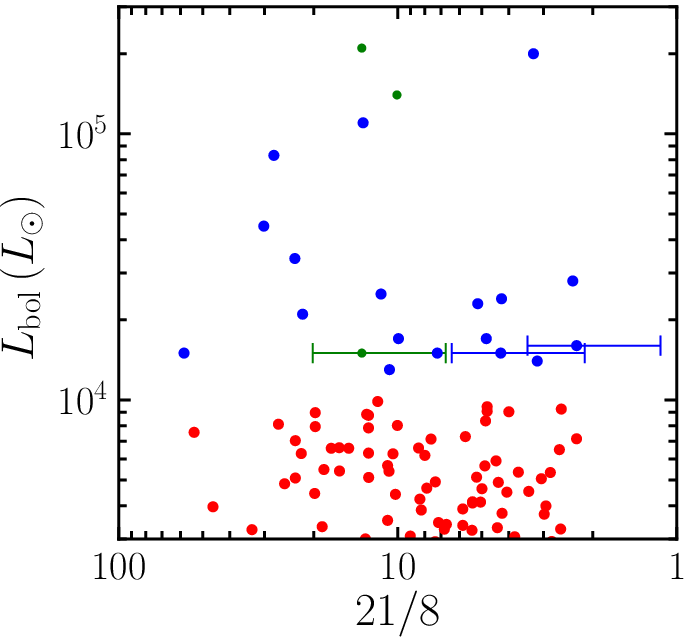
Figure 1: Sample selection plot where the luminosity (in units of L_⊙) is plotted against the MSX 21/8 $\mu$m color. Horizontal bars mark uncertainties in the color. While the blue sources fulfill our selection criteria, the red ones are below our luminosity cut of $10^{4}$ L_⊙. Green sources are those for which high-resolution mm data already exist and which were therefore excluded from the observations.

Regarding cluster formation and the early fragmentation processes, it is well established that high-mass stars typically form in a clustered mode with a high degree of multiplicity (e.g., Zinnecker & Yorke 2007; Bonnell et al. 2007a; Bressert et al. 2010; Peters et al. 2010; Chini et al. 2012; Peter et al. 2012; Krumholz 2014; Reipurth et al. 2014). Furthermore, the dynamical interactions between cluster members may even dominate their evolution (e.g., Gómez et al. 2005; Sana et al. 2012). High-spatial-resolution studies over the last decades have shown that most massive gas clumps do not remain single entities but fragment into multiple objects. However, the degree of fragmentation varies between regions (e.g., Zhang et al. 2009; Bontemps et al. 2010; Pillai et al. 2011; Wang et al. 2011; Rodón et al. 2012; Beuther et al. 2012; Palau et al. 2013; Wang et al. 2014; Csengeri et al. 2017; Cesaroni et al. 2017). The previous data indicate that high-mass monolithic condensations may be rare, but they could nevertheless exist (e.g., Bontemps et al. 2010; Csengeri et al. 2017; Sánchez-Monge et al. 2017). Going to sub-arcsecond resolution, most regions indeed fragment, but exceptions exist: For example, our recent investigations with the Plateau de Bure Interferometer (PdBI, now renamed to NOEMA) of the famous high-mass star-forming regions NGC7538IRS1 and NGC7538S revealed that NGC7538S has fragmented into several sub-sources at $\sim 0.3^{\prime\prime}$ resolution whereas at the same spatial resolution the central core of NGC7538IRS1 remains a single compact source (Beuther et al. 2012; see also Qiu et al. 2011 for more extended cores in the environment). At an even higher angular resolution of $\leq 0.2^{\prime\prime}$ or spatial scales below 1000 AU, Beuther et al. (2013) found that even the innermost structure of NGC7538IRS1 starts to fragment. This implies that the scales of fragmentation do vary from region to region. Other fragmentation studies do not entirely agree on the physical processes responsible for driving the fragmentation. For example, the infrared dark cloud study by Wang et al. (2014) indicates that turbulence may be needed to explain the large fragment masses. Similarly, Pillai et al. (2011) argue for two young pre-protocluster regions that turbulent Jeans fragmentation can explain their data. However, other studies like those by Palau et al. (2013, 2014, 2015) favor pure gravitational fragmentation. Similar results are also indicated in a recent ALMA study towards a number of hypercompact Hii regions (Klaassen et al., 2017). In addition to the thermal and turbulent gas properties, theoretical as well as observational investigations indicate the importance of the magnetic field for the fragmentation processes during (high-mass) star formation (Commerçon et al., 2011; Peters et al., 2011; Tan et al., 2013; Fontani et al., 2016). Furthermore, radiation feedback from forming protostars is also capable of reducing the fragmentation of the high-mass star-forming region (e.g., Krumholz et al. 2007).

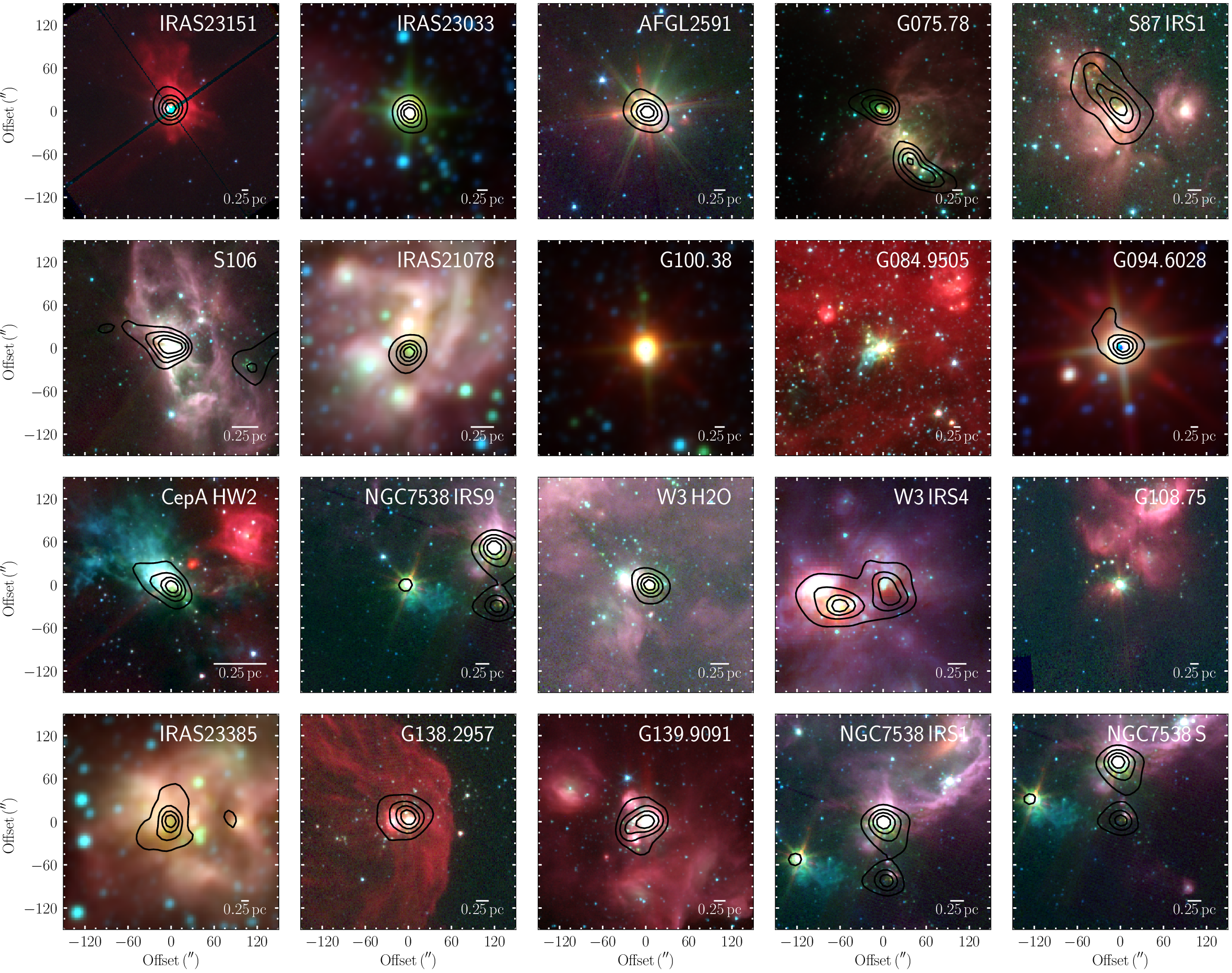
Figure 2: Large-scale overview images for the whole CORE sample. The color-scale show 3-color images with blue, green and red from Spitzer 3.6, 4.5 and 8.0 $\mu$m for all sources except IRAS 23033, IRAS21078, G100, G094 and IRAS 23385 for which WISE 3.4, 4.6 and 12 $\mu$m data are presented. Furthermore, W3IRS4 uses Spitzer 3.6, 4.5 $\mu$m and MSX 8 $\mu$m. The contours show SCUBA 850 $\mu$m continuum data (di Francesco et al. 2007; contour levels 20, 40, 60, 80% of the peak emission) for all sources except G100, G084 and G108 where these data do not exist.

It is important to keep in mind that fragmentation occurs on all scales, from large-scale molecular clouds down to the fragmentation of disks (e.g., Dobbs et al. 2014; André et al. 2014; Kratter & Lodato 2016). Different fragmentation processes may dominate on different spatial scales. In the continuum study presented here, we are concentrating on the fragmentation of pc-scale clumps into cores with sizes of typically several thousand AU. Smaller-scale disk fragmentation will also be addressed by the CORE program (see section 3) through the spectral line analysis of high-mass accretion disk candidates (e.g., Ahmadi et al., subm.).

The previous investigations of NGC7538IRS1 and NGC7538S (Beuther et al., 2012, 2013; Feng et al., 2016) can be considered as a pilot study for the CORE survey presented here. With an overall sample of 20 high-mass star-forming regions (see sample selection below) observed at uniform angular resolution ($\sim 0.3^{\prime\prime}-0.4^{\prime\prime}$) in the 1.3 mm wavelength band with NOEMA, we can investigate how (un)typical such fragmentation properties on core scales are. Fragmentation signatures to be investigated are, for example, the fragment mass, size and separation distributions, and how they relate to basic underlying physical processes.

In this paper, we present the sample selection, the general survey strategy as well as the observational characteristics. The rest of the paper will then focus on the continuum data and the fragmentation properties of the sample. The other scientific aspects of this survey will be presented in separate publications (e.g., Ahmadi et al. subm., Mottram et al. in prep., Bosco et al. in prep.).

2 Sample

Table 1: CORE Sample (grouped in track-sharing pairs)

Source	R.A.	Dec.	$\varv_{\rm{lsr}}$	$D$	$L$	$M^{a}$	$L/M$	$S_{8\mu m}$	$S_{21\mu m}$	IR-	a.f.e	Ref.
	(J2000.0)	(J2000.0)	$\left(\frac{\rm{km}}{\rm{s}}\right)$	(kpc)	($10^{4}$L⊙)	(M⊙)	$\left(\frac{\rm{L}_{\odot}}{\rm{M}_{\odot}}\right)$	(Jy)	(Jy)	bright
IRAS23151+5912	23:17:21.01	+59:28:47.49	-54.4	3.3	2.4	215b	112	23.8	101.1	+	b	d1,l2
IRAS23033+5951	23:05:25.00	+60:08:15.49	-53.1	4.3	1.7	495	34	5.0	24.0	–	a,b	d2,l1
AFGL2591	20:29:24.86	+40:11:19.40	-5.5	3.3	20.0	638	313	313.8	1023.4	+	a,b	d3,l1
G75.78+0.34	20:21:44.03	+37:26:37.70	-0.5	3.8	11.0	549	200	3.5	46.4	–	a,c	d4,l1
S87 IRS1	19:46:20.14	+24:35:29.00	22.0	2.2	2.5	1421	18	19.6	225.1	+	a	d5,l1
S106	20:27:26.77	+37:22:47.70	-1.0	1.3	3.4	47	723	53.1	1240.9	+	a,b	d6,l2
IRAS21078+5211	21:09:21.64	+52:22:37.50	-6.1	1.5	1.3	177	73	2.1	8.8	–	a,b	dl1
G100.3779-03.578	22:16:10.35	+52:21:34.70	-37.6	3.5	1.5	206d		12.9	92.7	+	b	d1,l2
G084.9505-00.691	20:55:32.47	+44:06:10.10	-34.6	5.5	1.3	648c	20	1.4	14.6	+	b	d2,l2
G094.6028-01.797	21:39:58.25	+50:14:20.90	-43.6	4.0	2.8	1525	18	63.9	150.5	+	b,c	d1,l2
CepAHW2	22:56:17.98	+62:01:49.50	-10.0	0.7	1.5	40	375	4.6	271.7	–	a,b,c	d7,l1
NGC7538IRS9	23:14:01.68	+61:27:19.10	-57.0	2.7	2.3	214	107	38.1	197.0	+	b	d7,l1
W3(H2O)	02:27:04.60	+61:52:24.73	-48.5	2.0	8.3	307	270	10.7	298.9	–	a,b,c	d8,l2
W3IRS4	02:25:31.22	+62:06:21.00	-42.8	2.0	4.5	481	93	15.4	465.2	+	a,b	d8,l1
G108.7575-00.986	22:58:47.25	+58:45:01.60	-51.5	4.3	1.4	6204d		6.9	21.9	+	b,c	d2,l3
IRAS23385+6053	23:40:54.40	+61:10:28.20	-50.2	4.9	1.6	510	31	1.6	3.5	–	b	dl2
G138.2957+01.555	03:01:31.32	+60:29:13.20	-37.5	2.9	1.4	197	71	9.1	90.0	+	a,b	d2,l1
G139.9091+00.197	03:07:24.52	+58:30:48.30	-40.5	3.2	1.1	349	32	12.9	282.2	+	a,b	d2,l1
Pilot study
NGC7538IRS1	23:13:45.36	+61:28:10.55	-57.3	2.7	21.0	1570	133	109.2	1468.6	+	a,b,c	d7,l1
NGC7538S	23:13:44.86	+61:26:48.10	-56.4	2.7	1.5	238	63	1.1	15.3	–	b,c	d7

^a Masses are calculated mainly from the SCUBA 850 $\mu$m fluxes by Di Francesco et al. (2008).
^b Based on 1.2 mm continuum data from Beuther et al. (2002)
^c Based on 1.1 mm continuum data from Ginsburg et al. (2013)
^d Based on C¹⁸O(3–2) data from Maud et al. (2015); effective radii for G100 $\sim$0.34 pc and for G108 $\sim$1.4 pc
^e Associated features (a.f.): a: cm continuum; b: H₂O maser; c: CH₃OH maser
References for distances and luminosities: d1: Choi et al. 1993, d2: Urquhart et al. 2011, d3: Rygl et al. 2012, d4: Ando et al. 2011, d5: Xu et al. 2009, d6: Xu et al. 2013, d7: Moscadelli et al. 2009, d8: Hachisuka et al. 2006; Xu et al. 2006, dl1: Molinari et al. 1996, dl2: Molinari et al. 1998
l1: RMS survey database (http://rms.leeds.ac.uk/cgi-bin/public/RMS_DATABASE.cgi), using SED fitting from Mottram et al. (2011) including Herschel fluxes and the latest distance determination
l2: RMS survey database (http://rms.leeds.ac.uk/cgi-bin/public/RMS_DATABASE.cgi), using SED fitting from Mottram et al. (2011) updated to the latest distance determination
l3: RMS survey database (http://rms.leeds.ac.uk/cgi-bin/public/RMS_DATABASE.cgi), calculated from the MSX 21 $\mu$m flux using the scaling relation derived by Mottram et al. (2011) and updated to the latest distance determination.

Our sample of young high-mass star-forming regions was selected to fulfill several criteria: (a) luminosities $>10^{4}$ L_⊙ indicating that at least an 8 M_⊙ star is forming, (b) distance-limited to below 6 kpc to ensure high linear resolution ($\sim$1000 AU), (c) high-declination sources (decl.$>$24^∘) to obtain the best possible uv-coverage (implying that they are either not at all or at most poorly accessible with the Atacama Large Millimeter Array, ALMA). Furthermore, only sources with extensive complementary high-spatial resolution observations at other wavelengths were selected to better characterize their overall properties. In this context, the sample is also part of a large e-Merlin project led by Co-I Melvin Hoare to characterize the cm continuum emission of the sample at an anticipated spatial resolution of down to 30 mas. The initial luminosity selection was based on luminosity and color-color criteria. Figure 1 presents the corresponding luminosity-color plot. We use the luminosity-color plot as a sample selection tool as the y- and x-axes act as proxies for stellar mass and evolutionary stage, respectively. By the time massive forming stars have reached $10^{4}$ L_⊙ the luminosity is determined primarily by the stellar mass as at this stage the accretion luminosity only contributes a small fraction of the total luminosity even at high accretion rates (e.g., Hosokawa & Omukai 2009; Hosokawa et al. 2010; Kuiper & Yorke 2013; Klassen et al. 2016). We also expect over time that the IR colors will evolve from red to blue as the envelope material is dispersed and/or accreted (e.g., Zhang et al. 2014).

Many sample sources are covered by the RMS survey (Red MSX sources, Lumsden et al. 2013), and a few additional prominent northern hemisphere regions are included as well. Our sample excludes the few sources that fulfill these selection criteria but which already have been observed at mm wavelengths with high angular resolution (e.g., W3IRS5, NGC7538IRS1/S, Rodón et al. 2008; Beuther et al. 2012). The resulting sample of 18 regions is complete within these described selection criteria. Because NGC7538IRS1 and NGC7538S were observed in an almost identical setup (only the compact D-array data were not taken), they are considered as a pilot study and their results are incorporated into the analysis of the CORE project. Table 1 presents a summary of the main source characteristics, including their local-standard-of-rest velocity $\varv_{\rm lsr}$, distance $D$, luminosity $L$, mass $M$ (see also section 5.3), their 8 and 21 $\mu$m fluxes, H₂O, CH₃OH maser and cm continuum associations as well as references for the distances and luminosities. Figure 2 shows a larger-scale overview of the twenty regions with the near- to mid-infrared data shown in color and the 850 $\mu$m continuum single-dish data (Di Francesco et al., 2008) presented in contours.

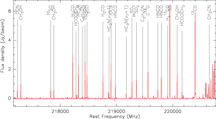
Figure 3: Example wide-band spectrum extracted toward AFGL2591. The most important lines in the bandpass are marked.

Regarding the evolutionary stage of the sample, they are all luminous and massive young stellar objects (MYSOs) or otherwise named high-mass protostellar objects (HMPOs). Subdividing the regions a bit further, some regions show very strong (sub)mm spectral line emission indicative of hot molecular cores (AFGL2591, G75.78+0.34, CepAHW2, W3(H₂O), NGC7538IRS1), other regions are line-poor (e.g., S87IRS1, S106, G100.3779, G084.9505, G094.6028, G138.2957, G139.9091), and the remaining sources exhibit intermediate-rich spectral line data. Furthermore, the sample covers various combinations of associated cm continuum, H₂O and class II CH₃OH maser emission (Table 1). Following Motte et al. (2007), we checked whether the sources belong to the so-called IR-bright or IR-quiet categories with the dividing line defined as IR-quiet when $S_{21\mu m}<10\rm{Jy}\left(\frac{1.7\rm{kpc}}{D}\right)^{2}\left(\frac{L}{1000\rm{L}_{\odot}}\right)$. In contrast to our initial expectation that all sources would classify as IR-bright, we clearly find some diversity among the sample (see Table 1). While the majority indeed qualified as IR-bright, a few sources fall in the IR-quiet category. Maybe slightly surprising, a few of our line-brightest sources are categorized as IR-quiet (e.g., CepA and W3(H₂O)). Therefore, the differentiation in these two categories only partly implies that the IR-quiet sources are potentially younger, but it suggests at least that these sources are still very deeply embedded into their natal cores. In this embedded stage, they are already capable of driving dynamic outflows, have high luminosities and produce a rich chemistry.

A different evolutionary time indicator sometimes used is the luminosity-over-mass ratio $L/M$ of the regions (see Table 1, e.g., Sridharan et al. 2002; Molinari et al. 2008, 2016; Ma et al. 2013; Cesaroni et al. 2017; Motte et al. 2017). The CORE sample covers a relatively broad range in this parameter space between roughly 20 and 700 L_⊙/M_⊙. However, this ratio is not entirely conclusive either. For example, the region with our lowest ratio (S87IRS1 with $L/M\sim 18$ L_⊙/M_⊙), that could be indicative of relative youth, is classified otherwise as IR-bright which seems counterintuitive at first sight. Since the various age-indicators are derived from parameters averaged over different scales, it is possible that they are averaging over sub-regions with varying evolutionary stages and are hence not giving an unambiguous evolutionary picture.

In summary, the CORE sample consists of regions containing HMPOs/MYSOs above $10^{4}$ L_⊙ from the pre-hot-core stage to typical hot-cores and also a few more evolved regions that have likely already started to disrupt their original gas core. The evolutionary stages are comparable to the sample by Palau et al. (2013, 2015) with the difference that they had a large fraction of sources below $10^{4}$ L_⊙ and even below $10^{3}$ L_⊙ (only four regions above $10^{4}$ L_⊙).

3 CORE large program strategy

Based on our experience with NGC7538IRS1 and NGC7538S (Beuther et al., 2012, 2013), we devised the CORE survey in a similar fashion. The full sample is observed in the 1.3 mm band, and a sub-sample of five regions will also subsequently be observed at 843 $\mu$m. Here we focus on the 1.3 mm part of the survey for the full sample. The shorter wavelength study will be presented after its completion.

Several aspects were considered to achieve the goals of the project: (i) The most extended A-configuration of NOEMA was used for the highest possible spatial resolution (ii) Complementary observations with more compact configurations of the interferometer recover information on larger spatial scales. Simulations showed that adding the B and D configurations provided the best compromise between spatial information and observing time. (iii) To also cover very extended spectral line emission, short spacing observations from the IRAM 30m telescope were added. (iv) Spectrally, among other lines our survey covers CH₃CN to trace high-density gas as might be found in accretion disks and/or toroids (e.g., Cesaroni et al. 2007) and H₂CO which traces lower-density, larger-scale structures. Both, CH₃CN and H₂CO are also well known temperature tracers (e.g., Mangum & Wootten 1993; Zhang et al. 1998; Araya et al. 2005). Furthermore, outflow tracers like ¹³CO and SO are included. A plethora of additional lines are also covered to investigate the chemical properties of the regions. An early example of such investigation can be found in the paper about the pilot study sources NGC7538IRS1 and NGC7538S by Feng et al. (2016).

Table 2: Spectral lines at high spectral resolution

Line	$\nu$	$E_{u}/k$
	(GHz)	(K)
H2CO$(3_{0,3}-2_{0,1})$	218.222	21
HCOOCH${}_{3}(17_{3,14}-16_{3,13})$	218.298	100
HC3N$(24-23)$	218.325	131
CH3OH$(4_{2,2}-3_{1,2})$	218.440	46
NH2CHO$(10_{1,9}-9_{1,8})$	218.460	61
H2CO$(3_{2,2}-2_{2,1})$	218.476	68
OCS$(18-17)$	218.903	100
HCOOCH${}_{3}(17_{4,13}-16_{4,12})$	220.167	103
CH2CO$(11_{1,11}-10_{1,10})$	220.178	77
HCOOCH${}_{3}(17_{4,13}-16_{4,12})$	220.190	103
CH3CN$(12_{6}-11_{6})$	220.594	326
CH${}_{3}^{13}$CN$(12_{3}-11_{3})$	220.600	133
CH${}_{3}^{13}$CN$(12_{2}-11_{2})$	220.621	98
CH3CN$(12_{5}-11_{5})$	220.641	248
CH3CN$(12_{4}-11_{4})$	220.679	183
CH3CN$(12_{3}-11_{3})$	220.709	133
CH3CN$(12_{2}-11_{2})$	220.730	98
CH3CN$(12_{1}-11_{1})$	220.743	76
CH3CN$(12_{0}-11_{0})$	220.747	69

With the wide-band correlator units WIDEX, a spectral range from 217.167 to 220.834 GHz was covered at a spectral resolution of 1.95 MHz, corresponding to a velocity resolution of $\sim$2.7 km s^-1 at the given frequencies. Figure 3 shows an example spectrum from AFGL2591. These wide-band units are used to extract the line-free continuum as well as to get a chemical census of the region. Furthermore, the velocity resolution is sufficient for outflow investigations. However, to study the kinematics of the central rotating structures, higher spectral resolution is required. Therefore, we positioned the eight narrow band correlator units to specific spectral locations covering the most important lines at a spectral resolution of 0.312 MHz, corresponding to a velocity resolution of $\sim$0.43 km s^-1 at the given frequencies. Table 2 shows the spectral lines covered at this high spectral resolution. For more details about the spectral line coverage we refer the reader to the CORE paper by Ahmadi et al. (subm.).

For the complementary IRAM 30 m short spacings observations, we mapped all regions with approximate map sizes of $1^{\prime}$ in the on-the-fly mode in the 1 mm band. Since the bandpasses at the 30 m telescope are broader and the receivers work in a double-sideband mode, the 30 m data cover a broader range of frequencies between $\sim$213 and $\sim$221 GHz in the lower sideband and between $\sim$229 and $\sim$236 GHz in the upper sideband. The line data that are covered by the NOEMA and 30 m observations can be merged and imaged together whereas the remaining 30 m bandpass data can be used as standalone data products. Since we do not use the single-dish data for the continuum study presented here, we refer to the CORE paper by Mottram et al. (in prep.) for more details on the IRAM 30 m data.

More details about the CORE project are provided at the team web-page at http://www.mpia.de/core. There, we will also provide the final calibrated visibility data and imaged maps. The data release will take place in a staged fashion: the continuum data are published now, the corresponding line data will be provided subsequently.

4 Observations

The entire CORE sample (except the pilot sources NGC7538IRS1 and NGC7538S) was observed at 1.37 mm between summer 2014 and January 2017 in the three PdBI/NOEMA configurations A, B and D to cover as many spatial scales as possible (see section 3). The baseline ranges for all tracks in terms of uv-radius are given in Table 3. The shortest baselines, typically between 15 and 20 m, correspond to theoretically largest recoverable scales of $16^{\prime\prime}-20^{\prime\prime}$. For each track, two sources were observed together in a track-sharing mode. The phase centers of each source and the respective source pairs for the track-sharing are shown in Table 1. Since each source was observed in three different configurations, at least three (half-) tracks were observed per source. Depending on the conditions, several source pairs were observed in more than three (partial) tracks in order to achieve the required sensitivity and uv-coverage. Altogether, this multi-configuration and multi-track approach resulted in excellent uv-coverage for each source, an example of which is shown in Fig. 4. Typically two phase calibrators were observed in the loops with the track-sharing pairs. For the final phase calibration, we mostly only used the stronger ones. Depending on array configuration and weather conditions, the phase noise varied between $\sim$10 and $\sim 50\deg$. Bandpass calibration was conducted with observations of strong quasars, e.g., 3C84, 3C273, or 3C454.3. The resulting spectral baselines are very good, over the broad WIDEX bandpass as well as the narrow-band bandpasses (e.g., see Fig. 3). The absolute flux calibration was conducted in most cases with the source MWC349 where an absolute model flux of 1.86 Jy at 220 GHz was assumed . For only very few tracks in which that source was not observed, the flux calibration was conducted with other well-known calibrators (e.g., LKH$\alpha$101). The absolute flux scale is estimated to be correct to within 20%.

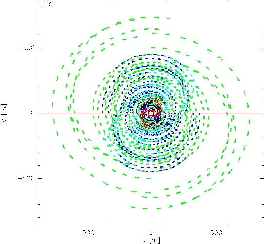
Figure 4: Example uv-coverage for CepA. The different colors correspond to different observed (half-)tracks. Red and black correspond to D-array observations, blue and cyan to B-array, and green to A-array data.

Table 3: CORE parameters

Source	Beam	lin. res.d	uv-radiuse	rms	rmssc	$5\sigma$	$S_{\rm{peak}}$	$S_{\rm{int}}$	mfa	$T$(H2CO)	$\Delta\varv$(H2CO)
	(′′, PA)	(AU)	(m)	($\frac{\rm{mJy}}{\rm{beam}}$)	($\frac{\rm{mJy}}{\rm{beam}}$)	(M⊙)	($\frac{\rm{mJy}}{\rm{beam}}$)	(mJy)	(%)	(K)	(km s-1)
IRAS23151	$0.45^{\prime\prime}\times 0.37^{\prime\prime}$(50∘)	1350	21-764	0.19	0.10	0.05	32.6	100	78	59	3.4
IRAS23033	$0.45^{\prime\prime}\times 0.37^{\prime\prime}$(47∘)	1760	20-765	0.46	0.28	0.28	38.9	310	64	55	3.5
AFGL2591	$0.47^{\prime\prime}\times 0.36^{\prime\prime}$(65∘)	1370	31-765	0.60	0.40	0.18	87.3	249	84	69	3.1
G75.78	$0.48^{\prime\prime}\times 0.37^{\prime\prime}$(60∘)	1615	21-765	0.60	0.42	0.16	64.7	256	87	108	5.3
S87IRS1	$0.54^{\prime\prime}\times 0.35^{\prime\prime}$(37∘)	980	16-765	0.23	0.21	0.06	33.7	214	87	48	3.7
S106	$0.47^{\prime\prime}\times 0.34^{\prime\prime}$(47∘)	530	19-765	1.25	0.62	0.02	73.9	170	87	135	4.8
IRAS21078	$0.48^{\prime\prime}\times 0.33^{\prime\prime}$(41∘)	650	34-765	0.60	0.28	0.03	34.7	1020	53	66	4.9
G100	$0.49^{\prime\prime}\times 0.33^{\prime\prime}$(56∘)	1440	16-765	0.08	0.05	0.03	8.5	67	–b	58	2.3
G084	$0.43^{\prime\prime}\times 0.38^{\prime\prime}$(69∘)	2230	15-753	0.10	0.08	0.22	6.2	85	67c	35	3.5
G094	$0.41^{\prime\prime}\times 0.39^{\prime\prime}$(77∘)	1600	15-762	0.14	0.11	0.36	13.6	90	81	18	2.5
CepA	$0.44^{\prime\prime}\times 0.38^{\prime\prime}$(80∘)	290	19-765	4.00	1.70	0.02	440.9	1225	72	119	5.3
NGC7538IRS9	$0.44^{\prime\prime}\times 0.38^{\prime\prime}$(80∘)	1110	19-765	0.30	0.15	0.04	41.2	237	76	86	4.0
W3(H2O)	$0.43^{\prime\prime}\times 0.32^{\prime\prime}$(86∘)	750	19-760	4.50	1.90	0.13	451.6	5292	25	162	6.6
W3IRS4	$0.45^{\prime\prime}\times 0.32^{\prime\prime}$(83∘)	770	19-762	0.60	0.60	0.11	39.3	377	87	66	4.2
G108	$0.50^{\prime\prime}\times 0.44^{\prime\prime}$(49∘)	2020	17-765	0.25	0.15	0.24	14.8	60	–b	36	3.3
IRAS23385	$0.48^{\prime\prime}\times 0.43^{\prime\prime}$(58∘)	2230	18-764	0.25	0.11	0.11	18.0	190	56	73	3.8
G138	$0.50^{\prime\prime}\times 0.41^{\prime\prime}$(60∘)	1320	20-764	0.16	0.16	0.12	6.2	100	82	36	2.9
G139	$0.51^{\prime\prime}\times 0.40^{\prime\prime}$(56∘)	1460	21-764	0.17	0.15	0.10	13.9	26	95	48	1.4
	previous pilot study
NGC7538IRS1	$0.33^{\prime\prime}\times 0.32^{\prime\prime}$(-55∘)	880	68-765	10.0	5.20	1.34	2334	2838	50	82	4.5
NGC7538S	$0.34^{\prime\prime}\times 0.31^{\prime\prime}$(-81∘)	880	68-765	0.60	0.50	0.14	28.1	253	91	78	5.6

The columns give the synthesized beam, the linear resolution, the baseline range (uv-radius), the rms noise before and after self-calibration, the $5\sigma$ mass sensitivity, the measured peak and integrated flux densities $S_{\rm{peak}}$ and $S_{\rm{int}}$, the missing flux ratios as well as the H₂CO derived temperatures $T$ and line widths $\Delta\varv$.
^a Missing flux, for details see main text
^b No single-dish data available
^c Based on BOLOCAM 1.1 mm flux measurement in $40^{\prime\prime}$ aperture (Ginsburg et al., 2013)
^d Average linear resolution
^e Projected uv baseline range

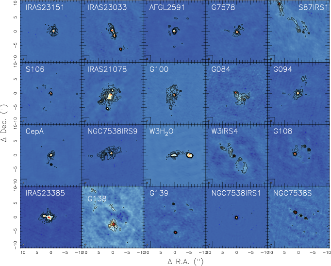
Figure 5: Compilation of 1.37 mm continuum images for CORE sample on the same angular scale. The contouring is in $5\sigma$ steps (see Table 3). The sources are labeled in each panel, and the synthesized beams are shown at the bottom-left of each panel. A comparison figure converted to linear scales is shown in Fig. 6. Zooms and absolute flux-scales are shown in Appendix B.

To achieve the highest angular resolution, uniform weighting was applied during the imaging process. The final synthesized beams for the continuum combining all NOEMA data vary between $\sim 0.32^{\prime\prime}$ and $\sim 0.5^{\prime\prime}$ with exact values for each source given in Table 3. The full width at half maximum of the primary beam of our observations is $\sim$22^′′. To create the continuum images, we carefully inspected the WIDEX bandpasses for each source individually and created the continuum from the line-free parts only. The $1\sigma$ continuum rms correspondingly varies from source to source. This depends not only on the chosen line-free channels, but also on the side-lobe noise introduced by the strongest sources in the fields. Although the uv-coverage is very good (Fig. 4), not all side-lobes can be properly subtracted, and the final noise depends on that as well.

To reduce calibration, side-lobe and imaging issues, we explored how much self-calibration would improve the data quality. For that purpose, we exported the continuum uv-tables to casa format and did the self-calibration within casa (version 4.7.2, McMullin et al. 2007). We performed phase self-calibration only, and the time intervals used for the process varied from source to source depending on the source strength. Solution intervals of either 220, 100 or 45 sec were used, where 45 sec is the smallest possible interval due to averaging of the data during data recording. Interactive masking during the self-calibration loops was applied, with only the strong peaks used in the first iterations and then subsequently adapted to the weaker structures. After the self-calibration, we again exported the data to gildas format and conducted all the imaging within gildas to enable direct comparisons with the original datasets. Again, uniform weighting was applied and we cleaned the data down to a $2\sigma$ threshold. To show the differences of the images prior to and after the self-calibration process, Appendix B presents the derived images before and after the self-calibration. The contouring is done in both cases in $5\sigma$ steps. Careful inspection of all data shows that no general structural changes were created during the self-calibration process. The self-calibration improved the data considerably with reduced rms noise and slightly increased peak fluxes. We find that the flux-ratios between the main sub-structures within individual regions remained relatively constant prior to and after self-calibration. In the rest of the paper, we will conduct the analysis with the self-calibrated dataset. Table 3 presents the $1\sigma$ continuum rms for all sources before and after self-calibration. We typically achieve sub-mJy rms with a range between 0.05 and 1.9 mJy beam^-1 for the 18 new targets. Only the pilot source NGC7538IRS1 has a slightly higher rms of $5.2\,$ mJy beam^-1 which can be attributed to the higher source strength and the missing D-array observations. Primary-beam correction was applied to the final images, and the fluxes were extracted from these primary-beam corrected data (section 5.2). Evaluating the measured peak flux densities $S_{\rm peak}$ and noise values (rms_sc) in Table 3 we find signal-to-noise ratios between 39 and 326 with the majority of region (13) exhibiting signal-to-noise ratios greater than 100. We are providing in electronic form the original pre-self-calibration images, the images after applying self-calibration as well as the primary-beam corrected images.

Simulated observations:

To better understand how the imaging affects our results, we simulated a typical observation. The details of the simulations can be found in Appendix A. To summarize the method and results: We used real single-dish dust continuum data from the large-scale SCUBA-2 850 $\mu$m map of Orion by Lane et al. (2016), converted the flux to 1.37 mm wavelength (assuming a $\nu^{3.5}$ frequency-relation), rescaled the spatial resolution and flux density to a distance of 3 kpc, and imaged different parts of Orion with the typical uv-coverage and integration time from the CORE project. Similar to our observations, the rms varied depending on whether a strong source (in this case Orion-KL) was present in the observed field. While the point source mass sensitivity is very good, between 0.01 and 0.1 M_⊙ (depending on the rms), with our spatial resolution typical Orion cores are extended structures, rather than point sources, even at a distance of 3 kpc. Hence, the dependence of the rms noise on the strongest sources in the field strongly affects the actual core mass sensitivity for extended structures as well. Taking the two examples shown in Appendix A, cores with masses down to $\sim$1 M_⊙ are detectable in fields without very strong sources. If such a low-mass core were within the stronger Orion-KL field, it would not be detectable anymore. Therefore, the core mass sensitivities strongly depend on the strongest and most massive sources within the respective observed fields. The dynamic range limit of the simulations of Orion-KL is approximately 53.

5 Continuum structure and fragmentation results

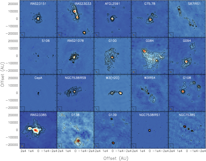
Figure 6: Compilation of 1.37 mm continuum images for CORE sample converted to linear resolution elements. The contouring is in $5\sigma$ steps (see Table 3). The sources are labeled in each panel, and the synthesized beams are shown at the bottom-left of each panel.

5.1 Source structures

Figures 5 and 6 present the 1.37 mm continuum data of the full CORE sample. While Fig. 5 shows the data in angular resolution over the full area of the primary beam of the observations, Fig. 6 uses the distances of the sources (Table 1) and presents the data at the same linear scales, making direct comparisons between sources possible. The first impression one gets from these dust continuum images is that the structures are far from uniform. While some sources are dominated by single cores (e.g., IRAS23151, AFGL2591, S106, NGC7538IRS1), other regions clearly contain multiple cores with a lot of substructures (e.g., S87IRS1, IRAS 21078, W3IRS4), some of which have more than 10 cores within a single observed field (see section 5.2). We see no correlation between the number of fragments and the distances to the sources. We will discuss this fragmentation diversity in more detail in section 6.

5.2 Source extraction

To extract the sources from our 20 images, we used the classical clumpfind algorithm by Williams et al. (1994) on our self-calibrated images. As input parameters we used the $5\sigma$ contour levels presented in Figures 5 and 6 as well as in Appendix B. These images sometimes also show negative $5\sigma$ contours, indicating that the interferometric noise is neither uniform nor really Gaussian. Therefore, we inspected all sources identified by clumpfind individually and only included those where the peak flux density is $\geq$10$\sigma$ (two positive contours minimum in Appendix B). The derived positional offsets from the phase center, peak flux densities $S_{\rm{peak}}$, integrated flux densities $S_{\rm{int}}$ and equivalent core radii (calculated from the measured core area assuming a spherical distribution) are presented in Table LABEL:mass_flux ($S_{\rm{peak}}$ and $S_{\rm{int}}$ are derived from the primary-beam corrected data).

To estimate the amount of missing flux filtered out by the interferometric observations, we extracted the 850 $\mu$m peak flux densities from single-dish observations, mainly from the SCUBA legacy archive catalogue (Di Francesco et al., 2008). Since this dataset has a final beam size of $22.9^{\prime\prime}$ it covers our primary beam size very well. Scaling this 850 $\mu$m data with a typical $\nu^{3.5}$ dependency to the approximate flux at our observing frequency of 220 GHz, we can compare these values to the sum of the integrated fluxes measured for each target region from our previous clumpfind analysis. Table 3 presents the corresponding missing flux values (mf in percentage) for the sample (for two regions – G100 & G108 – we did not find corresponding single-dish data). The amount of missing flux varies significantly over the sample, typically ranging between 60 and 90%. The only extreme exception is W3(H₂O) where only 25% of the flux is filtered out. This implies that for this region the flux is strongly centrally concentrated without much of a more extended envelope structure. For the remaining sources, even with the comparably good uv-coverage (Fig. 4) a significant fraction of the flux is filtered out. The variations from source to source indicate that the spatial density structure varies strongly from region to region as well (see also discussion in section 6).

There is a broad distribution in the number of cores identified in each region. We find between 1 and 20 cores among the different regions (see Table 4). To check whether this range of identified cores is related to our mass sensitivity, in Figure 7 we plot the 5$\sigma$ mass sensitivity (Table 3 and section 5.3) versus the number of identified cores (excluding NGC7538IRS1 because of its unusually poor mass sensitivity limit, Table 3). While there might be a slight trend of more cores towards lower mass sensitivity limits, our lowest mass sensitivity limit region CepA also shows only two cores. In the main regime of $5\sigma$ mass sensitivities between 0.1 and 0.3 M_⊙ we do not see a relation between the number of identified cores and the mass sensitivity. Hence, the number of identified cores does not seem to be strongly dependent on our mass sensitivity limits below 0.4 M_⊙.

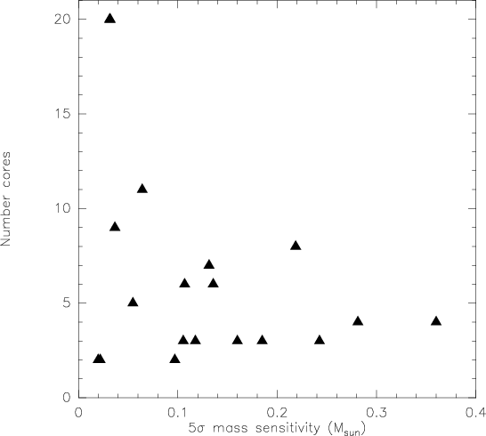
Figure 7: Number of identified cores plotted against the $5\sigma$ mass sensitivity. NGC7538IRS1 is excluded because of its unusually high mass sensitivity limit).

5.3 Mass and column density distributions

Assuming optically thin dust continuum emission at 220 GHz, we can estimate the gas masses and peak column densities for all identified cores in the sample. Following the original outline by Hildebrand (1983) in the form presented by Schuller et al. (2009), we use a gas-to-dust mass ratio of 150 (Draine, 2011), a dust mass absorption coefficient $\kappa$ of 0.9 cm²g^-1 (Ossenkopf & Henning 1994 at densities of $10^{6}$ cm^-3 with thin ice mantles) and average temperatures for each region derived from the CORE IRAM 30m H₂CO data. H₂CO is a well-known gas thermometer in the interstellar medium (Mangum & Wootten, 1993), and we derive beam-averaged temperatures from the single-dish spectra toward the peak positions of each region at a spatial resolution of $11^{\prime\prime}$. For the temperature estimates we fitted the data with the xclass tool (eXtended casa Line Analysis Software Suite) tool (Möller et al., 2017). xclass models the spectra by solving the radiative transfer equation for an isothermal homogeneous object in local thermodynamic equilibrium (LTE), using the molecular databases VAMDC and CDMS (http://www.vamdc.org and Müller et al. 2001). xclass employs the model optimizer package magix (Modeling and Analysis Generic Interface for eXternal numerical codes) to find the best fit solutions (Möller et al., 2013). The derived temperatures are shown in Table 3. Since we are deriving beam-averaged temperatures from the single-dish data, the actual temperatures of individual cores at smaller spatial scales may vary compared to that. More detailed temperature analysis from the combined interferometer plus single-dish data is beyond the scope of this paper and will be conducted in future work on the CORE data. The mass estimates are in general lower limits since we are filtering out large-scale flux that may be associated with the dense cores (see also Appendix A). Furthermore, while the optically thin assumption for the dust emission should be valid in most cases, there may be some exceptions like CepA where high peak flux densities (Tables 3 & LABEL:mass_flux) imply high brightness temperatures indicating moderate optical depth at these peak positions. However, since the masses are calculated typically over areas larger than just the peak, and the brightness temperatures decrease quickly with distance from the peak, this effect should be comparably weak.

The derived core masses and column densities are presented in Table LABEL:mass_flux and roughly span 0.1 to 40 M_⊙, and $5\times 10^{22}$ to $10^{25}$ cm^-2. For the mass and column density analysis, we excluded sources for which the continuum emission is clearly dominated by Hii regions and hence show barely dust continuum emission. These are specifically W3(OH) (cores #1 and #2 in W3(H₂O), the southern ring-like region in W3IRS4 (sources #5 and #6) and core #2 in S87IRS1. For several other cores, the fluxes were corrected for free-free emission for the mass determinations (see Table LABEL:mass_flux).

Using similar assumptions, we also re-estimated the large-scale mass reservoir for the sample. For most sources, we used the integrated 850 $\mu$m fluxes derived by Di Francesco et al. (2008), while for IRAS 23151 the 1.2 mm flux was derived from the MAMBO data presented in Beuther et al. (2002), and for G084 we used the 1.1 mm BOLOCAM data from Ginsburg et al. (2013). The used gas-to-dust mass ratio and average H₂CO derived temperatures are the same as above, and we used for the single-dish data dust absorption coefficients $\kappa$ of 0.78, 0.9 and 1.4 cm²g^-1 at 1.2, 1.1 and 0.85 mm wavelengths, respectively (Ossenkopf & Henning 1994 at densities of $10^{5}$ cm^-3). The derived total masses are presented in Table 1 (for G100 and G108, the masses are taken from C¹⁸O(3–2) data from Maud et al. 2015). While the regions have typical mass reservoirs of several 100 M_⊙, the sample spans a comparably broad range between $\sim$40 and $\sim$1500 M_⊙ (for G108 even higher masses are measured, however over a comparably large area with radius 1.4 pc, Table 1 and Maud et al. 2015).

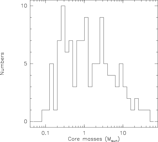
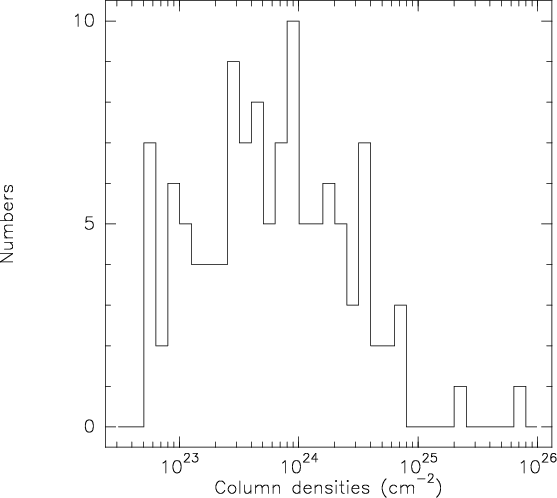
Figure 8: Histograms of masses (top panel) and column densities (bottom panel) for all detected cores.

For the NOEMA-only derived core parameters, Figure 8 shows histograms of the masses and column densities. The combined mass distribution shows that most detected cores are in the range between $\sim$0.1 and $\sim$10 M_⊙ with only a few cores exceeding 10 M_⊙. The most massive core is in NGC7538IRS1 with 43 M_⊙ (although significant free-free contamination may affect the estimate for this source, Beuther et al. 2012). Regarding the cores in excess of 10 M_⊙, there is no clear trend whether they are found as isolated objects or embedded in fragmented regions. For example, comparably massive cores are found in the low-fragmentation regions NGC7538IRS1 or AFGL2591, but cores of similar mass are also found in more fragmented regions like IRAS 23151, IRAS 23033, G75.78, as well as in the intermediately fragmented region W3(H₂O). The peak column densities are very large, typically exceeding $10^{23}$ cm^-2 and even going above $10^{25}$ cm^-2 for a few exceptional regions. Figure 9 plots the column densities against the masses, and while we see a scatter, there remains nevertheless a trend that column densities and masses are correlated. If one takes into account the distance-dependencies of our derived parameters (color-coding in Fig. 9), we see that the higher-mass-lower-column-density sources are found on average at larger distances. With increasing distance the physical size of the beam, where the column density is measured within, increases as well. Such larger area beams cover the central highest-column-density peak position but also more lower-column-density environmental gas. This smoothing slightly decreases the measured column densities with increasing distance. The other way round, increasing the covered area with distance also increases the measured masses. Hence, part of the scatter in Fig. 9 is caused by the distance range of our sample. For smaller distance bins, the scatter is significantly reduced.

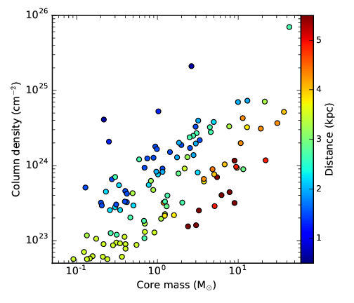
Figure 9: Gas column densities versus masses for all detected cores. The color-coding shows the distances of the sources.

Using the derived equivalent radii of the cores from the clumpfind analysis (Table LABEL:mass_flux), we can also derive mean densities for all cores under the assumption of spherical symmetry. Figure 10 plots these mean densities against the corresponding core masses, again color-coded with distance. While these average densities are rather high, typically between $10^{6}$ and $10^{8}$ cm^-3, there is no clear trend between the densities and the masses. Taking again the distances into account the scatter is reduced but identifying trends within distance-limited ranges is still difficult. Hence, in this sample, the core densities are similar over the whole range of observed core masses. Having a correlation between mass and column density but less good correlation between mass and average density implies that the core masses should correlate with their sizes, i.e., equivalent radii. Figure 11 presents the corresponding data again color-coded with distance. And indeed mass and size are well correlated for the sample, again much tighter if one looks at limited distance ranges. Figure 11 also plots lines of constant column densities between $10^{23}$ and $10^{25}$ cm^-2. While most regions scatter between the $10^{23}$ and $10^{24}$ cm^-2 lines, also sub-samples between limited distance ranges do not follow constant column density distributions but increase in column density with increasing mass, as already shown in Fig. 9.

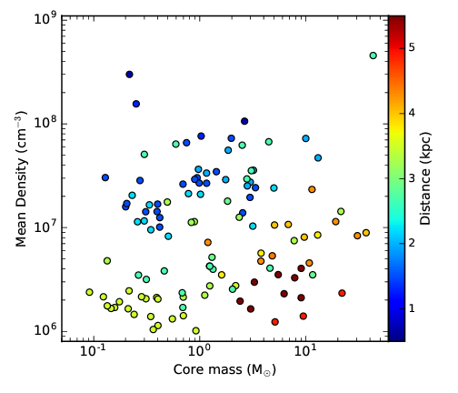
Figure 10: Mean core densities versus masses for all detected cores. The color-coding shows the distances of the sources.

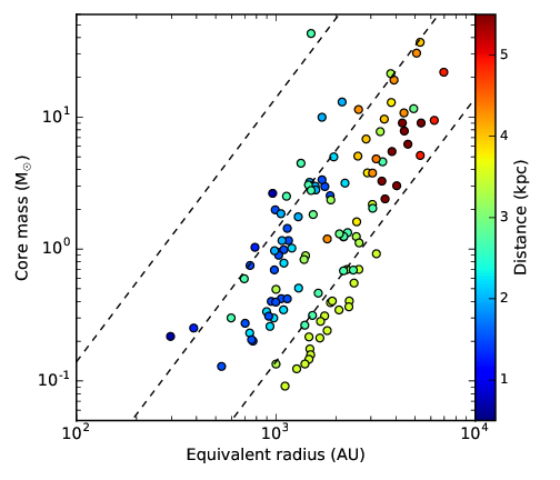
Figure 11: Core masses versus equivalent radii for all detected cores. The color-coding shows the distances of the sources. The dashed lines show constant column density with levels of $10^{23}$, $10^{24}$ and $10^{25}$ cm^-2 from right to left.

To estimate the typical Jeans fragmentation lengths and masses for the clump scales, we assume mean densities of the original larger-scale parental gas clumps between $10^{5}$ and $10^{6}$ cm^-3 (e.g., Beuther et al. 2002; Palau et al. 2014) and a temperature range between 20 and 50 K, typical for regions in the given evolutionary stages. For such conditions, the estimated Jeans length is between $\sim$5500 and 27700 AU. For comparison, the corresponding Jeans masses in this parameter range vary between 0.3 and 3.5 M_⊙. While a large fraction of the core masses lies within the regime of the Jeans masses, a non-negligible number of sources also have higher masses ($\sim 36\%$) in excess of the Jeans mass of the original cloud. Since our mass estimates are lower limits, even more cores may exceed the estimated Jeans masses. However, since the mass estimates are affected by many uncertainties (in addition to the missing flux, the assumed dust properties and temperatures are adding an uncertainty of factors 2-4), the core separations may be a better proxy for analyzing the fragmentation properties of the gas clumps.

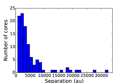
Figure 12: Nearest neighbor separation histogram from minimum spanning tree analysis

5.4 Core separations

To quantify the core separations in all 20 sample regions, we employed the minimum spanning tree algorithms available within the astroML software package (VanderPlas et al., 2012) which determines the shortest distances that can possibly connect each of the cores in the sampled field. From this, the minimum, maximum and mean separations of the cores in each field were determined, and are presented in Table 4, with the distribution of nearest neighbor separations shown in Figure 12. Since our data are 2D projections of 3D distributions, these measured separations are necessarily lower limits. The minimum core separations are typically on the order of a few 1000 AU (peak at $\sim$2000 AU, similar to Palau et al. 2013) with only a few core separations for the most nearby sources being measured below 1000 AU. However, this lower limit is most likely not a real physical lower separation limit but associated with the spatial resolution. With typical resolution elements around $0.3^{\prime\prime}-0.4^{\prime\prime}$ (Table 3) at distances of several kpc (Table 1), the linear spatial resolution is below 1000 AU for the most nearby sources (Table 3).

In contrast to likely not resolving all sub-structures within the regions, we nevertheless observe strong fragmentation in many targets. In particular, given the above estimated Jeans length between $\sim$5500 and 27700 AU (depending on density and temperature), most regions appear to fragment at or below this thermal Jeans length scale. Alternatively, the cores could have initially fragmented on Jeans length scales, and then the fragments could have approached each other even further due to the ongoing bulk motions from the global collapse of the regions. In contrast to that, the turbulent Jeans analysis, which includes the turbulent contributions to the sound speed, results in significantly larger mass and length scales (e.g., Pillai et al. 2011; Wang et al. 2014) than the classical thermal Jeans analysis.

Table 4: Linear Minimum Spanning Tree Analysis

Source	#cores	mean sep	min sep	max sep
		(AU)	(AU)	(AU)
IRAS23151	5	3763	2195	5264
IRAS23033	4	12185	5124	22616
AFGL2591	3	15012	8284	21739
G75.78	4	4392	3202	5924
S87IRS1	11	4564	1728	18625
S106	2	5029	5029	5029
IRAS21078	20	1482	710	2491
G100.3779	20	3027	1573	7247
G084.9505	8	6810	4247	9406
G094.6028	4	9175	4521	18397
CepAHW2	2	2382	2382	2382
NGC7538IRS9	9	3087	1558	4524
W3H2O	7	2583	1410	6071
W3IRS4	6	3785	1069	7298
G108.7575	3	13774	8341	19206
IRAS23385	3	7413	6918	7909
G138.2957	3	22088	16537	27640
G139.9091	2	32468	32468	32468
NGC7538IRS1	1
NGC7538S	6	7828	1520	13663

6 Discussion

Fragmentation occurs in general on various spatial scales and is likely a hierarchical process. Within our CORE project, we investigate the fragmentation processes on clump scales in high-mass star-forming regions. We concentrate on the dense central structures on scales above $\sim$1000 AU and roughly below 50000 AU or 0.25 pc. These largest scales correspond roughly to the largest theoretically recoverable scales with 15 m baselines at 3 kpc distance (section 4). In the continuum study presented here we investigate the fragmentation of clumps into cores. Fragmentation on smaller disk-like scales will also be investigated by the CORE program, however, that is more strongly based on the spectral line data and will be discussed in complementary papers (e.g., Ahmadi et al. subm., Bosco et al. in prep.).

6.1 Thermal versus turbulent fragmentation

With respect to the fragmentation of massive gas clumps, some important questions are: What controls the fragmentation properties of high-mass star-forming clumps? Is thermal Jeans fragmentation sufficient? How important are additional parameters like an initial non-uniform density profile or the magnetic field properties? How important is global accretion onto the clump from the diffuse ISM?

Regarding turbulent and thermal contributions, a number of studies have investigated this problem. For example, Wang et al. (2014) found that the observed masses of fragments within massive infrared dark cloud clumps are often more than 10 M_⊙. These masses are an order of magnitude larger than the thermal Jeans mass of the clump. Therefore they argue that the massive cores in a protocluster are more consistent with turbulent Jeans fragmentation (i.e., including a turbulent contribution to the velocity dispersion). Similar results were found by Pillai et al. (2011) in their study of two young pre-protocluster regions. On the other hand, Palau et al. (2013, 2014, 2015) found in their compiled sample of more evolved (IR-bright) star-forming regions that the masses of most of the fragments are comparable to the expected thermal Jeans mass, while the most massive fragments have masses a factor of 10 larger than the Jeans mass. Palau et al. (2013, 2014, 2015) concluded that these objects are consistent with thermal Jeans fragmentation of the parental cloud, in agreement with recent other investigations (e.g., Henshaw et al. 2017; Cyganowski et al. 2017). Recent ALMA studies of regions containing hypercompact Hii regions also show small fragment separation scales (Klaassen et al., 2017). In addition to this, Fontani et al. (2016) argue that the magnetic field is important for the fragmentation of IRAS 16061–5048c1 (see also Commerçon et al. 2011; Peters et al. 2011).

In our sample of high-mass star-forming regions, including regions in an evolutionary stage comparable to those studied by Palau et al. (2013, 2014, 2015), we find that most of the fragment masses approximately agree with a plausible range of Jeans masses, and most nearest-neighbor separations are below the predicted scales of thermal Jeans fragmentation. To explore that in more detail, Fig. 13 plots the derived core masses against the nearest neighbor separation derived from the minimum spanning tree analysis. The full and dashed lines show the relation between both thermal Jeans mass and Jeans length depending on density and temperature. In general, we do not find a clear trend between the two properties, and distance does not seem to be the primary factor in the observed scatter either. The Figure also shows that for the plausible range of densities and temperatures ($10^{5}$ to $10^{7}$ cm^-3 and 10 to 100 K) the observed parameters are difficult to explain. One has to keep in mind that both observables are lower limits: the mass because of missing flux and the separation because of projection effects. Accounting for these effects, the measurements could shift a bit closer to the predicted lines, but could also shift sources parallel to them. For comparison, in the turbulent Jeans fragmentation picture, the sound speed is replaced by the velocity dispersion (e.g., Wang et al. 2014), which is typically a factor 5 to 10 higher than the thermal sound speed (see H₂CO line width $\Delta v$(H₂CO) in Table 3). Even if not all the observed line width is caused by pure turbulent motions, but also has contributions from organized motions due to, e.g., large-scale infall, the regions clearly exhibit turbulent motions. Since the Jeans length and mass depend to the first and third power on the sound speed, respectively, replacing the thermal sound speed with the turbulent sound speed would shift the drawn correlations in Fig. 13 largely outside the observed box beyond the top-right corner. While we cannot conclude that thermal fragmentation explains everything, our data seem to refute that a turbulent contribution is needed if one applies a simple Jeans analysis for these spatial scales.

Several factors contributed to the apparent difference in fragmentation analysis between Wang et al. (2014) or Pillai et al. (2011) on the one side, and Palau et al. (2013, 2014, 2015) and the study here on the other side. First, the Wang et al. (2014) sample, incorporating data from Zhang et al. (2009) and Zhang & Wang (2011), has a typical $1\sigma$ mass sensitivity of 1 $M_{\odot}$. Therefore, lower mass fragments close to the global Jeans mass were not detected in these observations. Indeed, more sensitive observations from ALMA toward one of the objects in the sample, IRDC G28.34, revealed lower mass fragments (Zhang et al., 2015). Secondly, time evolution must play a role since fragmentation is a continuous process. As mentioned in section 5.4, the separation scales between fragments may also change with evolutionary time. In the picture of globally collapsing clouds and gas clumps, one would expect larger fragment separation at early evolutionary stages. Then, during the ongoing collapse, the fragments may move closer together, following the overall gravitational contraction of the region. Therefore, the observed state of fragmentation only represents a snapshot in the time evolution. The less evolved regions such as those in Wang et al. (2014) or Pillai et al. (2011) may present a deficit of low-mass fragments because the typical density of the cloud/clump is still lower so that a distributed low-mass protostar population may not have formed yet (e.g., Zhang et al. 2015). Furthermore, the more evolved objects such as those in this paper here have higher densities (Fig. 10), and therefore experience more fragmentation and are potentially more advanced in forming low-mass protostars.

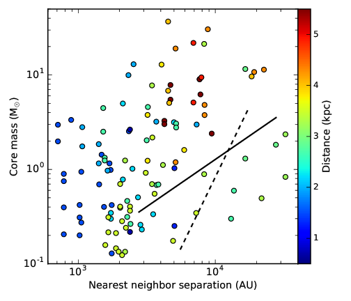
Figure 13: Fragment masses against nearest neighbor separation from the minimum spanning tree analysis. The full line corresponds to the Jeans lengths and Jeans masses calculated at 50 K for a density grid between $10^{5}$ and $10^{7}$ cm^-3. For comparison, the dashed line corresponds to the Jeans lengths and Jeans masses calculated at a fixed density of $5\times 10^{5}$ cm^-3 (Beuther et al., 2002) with temperatures between 10 and 100 K. The color-coding shows the distances of the sources.

In addition to the presented fragmentation properties, we point out that the nearest separations of cores are peaking around the spatial resolution limit of the observation (Fig. 12). Hence, fragmentation is also expected on even smaller scales. This can be investigated for this sample by higher spatial resolution observations with the future upgraded NOEMA (the baselines lengths are expected to be doubled), and for more southern sources with ALMA.

Recently, Csengeri et al. (2017) reported limited fragmentation for earlier evolutionary stages based on Atacama Compact Array data at $3.5^{\prime\prime}-4.6^{\prime\prime}$. At the given spatial resolution and a mass sensitivity $>11$ M_⊙ they find that in 77% of their sample only three or fewer massive cores are found. However, because of the lower angular resolution and worse mass sensitivity, a direct comparison between their and this study is not possible. The data of Csengeri et al. (2017) are complemented with ALMA 12 m array data, and the combined dataset will be very valuable for comparison with the CORE project.

A different aspect to be considered is that the fragmentation properties likely change with spatial scale. Kainulainen et al. (2013, 2017) have shown for two filaments (the infrared dark cloud G11.11 and the Orion integral shape filament) that the fragmentation properties appear to show distinct signatures at different spatial scales. In particular for the infrared dark cloud, Kainulainen et al. (2013) argue that filament fragmentation dominates on large spatial scales ($\geq 1$ pc), whereas on smaller spatial scales thermal Jeans fragmentation takes over ($\sim 0.2$ pc). With respect to our CORE sample, analyzing the filamentary properties on larger spatial scales is beyond the scope of this paper. However, it is clear that the CORE study deals with massive star-forming regions at high densities and not with the larger-scale, potentially filamentary clouds. In relation to the work by Kainulainen et al. (2013, 2017), we are in the second regime that would be dominated by Jeans fragmentation. Therefore, our general result that the CORE sample is more consistent with thermal Jeans fragmentation is in agreement with the results by Kainulainen et al. (2013, 2017).

6.2 Fragmentation diversity

Our sample clearly shows that the fragmentation properties within high-mass star-forming regions are not uniform, finding a diversity from highly fragmented regions to those that host one or only very few cores (see also Bontemps et al. 2010; Palau et al. 2013; Csengeri et al. 2017). While this sample seems in general largely consistent with thermal Jeans fragmentation (see previous subsection), it should be noted that we also find a few massive cores in excess of 10 M_⊙ (sec. 5.3 and Fig. 8). A high level of fragmentation with many low-mass cores favors high-mass star formation scenarios in the framework of competitive accretion (e.g., Clark & Bonnell 2006; Bonnell et al. 2007b; Smith et al. 2009), whereas individual massive cores are more strongly needed in the turbulent core picture (e.g., McKee & Tan 2003; Tan et al. 2014). Because we find examples for both pictures in our CORE sample, this may indicate that different high-mass star formation scenarios are possible or even interplay with each other.

Since the sample is selected to host high-mass protostellar objects (HMPOs), the range of evolutionary stages is not broad. Nevertheless, as discussed in section 2, within the HMPO category, we cover regions with varying IR-brightness and luminosity-to-mass ratios. Hence, while evolution is unlikely to be the main explanation for the observed fragmentation diversity, it cannot be entirely excluded. Furthermore, as discussed in the previous subsection, different levels of initial turbulence are also unlikely to be the underlying cause. Other possibilities to explain the different levels of fragmentation are variations in the initial density profiles and/or variations in the magnetic field properties. Differences in the density profiles could also arise from environmental effects like global collapse where the central gas clumps are continuously fed by some larger-scale cloud envelope.

Since the whole sample is observed with rather uniform uv-coverages, one wonders whether the amount of missing flux may be related to density structure of the parental gas clump and by that to the observed fragmentation properties of the cores. Therefore, we compare a few extreme cases: The two comparably isolated regions AFGL2591 and NGC7538IRS1 (both at similar distances at 3.3 and 2.7 kpc, Table 1) show very different amounts of missing flux with values of 84% and 50% of the flux being filtered out. At the other extreme, two highly fragmented sources like S87IRS1 and IRAS21078 (at distances of 2.2 and 1.5 kpc, Table 1) also exhibit very different values of 87% and 53% of flux being filtered out. Hence, the overall fraction of flux being lost because of the interferometric observations – or rather the amount of mass in a diffuse, larger-scale reservoir – appears not to be an important issue for the observed fragmentation differences.

Girichidis et al. (2011) have shown with simulations of star-forming regions how the density profile affects the level of fragmentation: While flat profiles ($\rho\propto$constant) resulted in many fragments, they find that density profiles like $\rho\propto r^{-2}$ (over cloud radii of $\sim$0.1 pc) quickly lead to the formation of a single object at the center where further fragmentation is prohibited. In their simulations, the intermediate case with $\rho\propto r^{-1.5}$ is also dominated by a central object but additional fragments can form depending on their initial turbulence field. Observations of the density profiles of high-mass gas clumps by different groups typically find density slopes $\rho\propto r^{-\alpha}$ with $\alpha$ between 1.5 and 2.6 (e.g., Beuther et al. 2002; Mueller et al. 2002; Fontani et al. 2002; Hatchell & van der Tak 2003). Furthermore, Palau et al. (2014) find a weak inverse trend between level of fragmentation and steepness of density profile, i.e., less fragmentation for steep density profiles. Hence, it seems reasonable that a range of initial density profiles can at least partly explain the observed diversity of fragmentation properties in our CORE sample. In future work, we are going to follow up on that and will investigate the density structure of the regions based on the combination of single-dish data with the interferometer data in more depth.

In addition to this, different magnetic field properties in the parental gas clumps can cause similar effects. Typically, the ratio between gravity and magnetic field is phrased in terms of the critical mass-to-flux ratio (e.g., Tilley & Pudritz 2007). Commerçon et al. (2011) modeled the collapse of high-mass star-forming regions with a range of magnetic field strengths. While their low-magnetic field case results in a larger number of fragments, the high-magnetic field case is dominated by a central massive object (see also Fontani et al. 2016). Similarly, Peters et al. (2011) also find reduced fragmentation with increasing magnetic field strength. To really differentiate whether the initial density profile and/or magnetic field properties are the dominant reason explaining the observed fragmentation diversity, we need to know the magnetic field strength as well as the initial density profile. For two regions within the CORE sample (W3(H₂O) and NGC7538IRS1) magnetic field studies have already been conducted with the Submillimeter Array on arcsecond resolution scale (Chen et al., 2012; Frau et al., 2014). The derived magnetic field strengths are comparably high in both regions with 17.0 and 2.5 mG, respectively. Since both regions exhibit very few or even only one fragment, the observed high magnetic field values are consistent with the low degree of fragmentation in these two regions. Future investigations in this direction are anticipated for the whole sample, which in particular will reveal whether regions with a high degree of fragmentation have a lower magnetic field strength.

7 Conclusions and Summary

With the goals of studying the fragmentation, disk formation, outflows and chemical properties during the birth of the most massive stars, we have conducted the IRAM NOEMA large program CORE, observing a sample of 20 high-mass star-forming regions at $0.3^{\prime\prime}-0.4^{\prime\prime}$ resolution in the 1.37 mm continuum and spectral line emission. In this paper, we present the survey scope, its main observational characteristics, the sample selection and the overall goals of the project. More details about the project as well as the first data release of the continuum data are provided at http://www.mpia.de/core. For a first scientific analysis of the data, we concentrated on the 1.37 mm dust continuum emission to investigate the fragmentation properties during early high-mass cluster formation.

We observe diverse fragmentation morphologies ranging from regions that are dominated by single high-mass cores to those that fragment into up to 20 cores. Since the sample contains mainly high-mass protostellar objects (although with some range of evolution within that category), larger-scale evolutionary effects are unlikely to explain all the differences. Observational artifacts like interferometric missing flux or different physical resolution can also be ruled out. The typical nearest neighbor separations peak below the thermal Jeans length determined from estimates of the initial average cloud density, indicating that thermal gravitational fragmentation is sufficient to explain the main observed core separations, and that additional turbulent contributions to the Jeans analysis are not needed for this sample. The diversity between regions with few or only one fragment versus those with many fragments may be explained by differences in the initial density structures of the maternal gas clumps (potentially caused by environmental effects like global gas infall from a surrounding envelope) and/or variations in the initial magnetic field configurations. Since the nearest neighbor separation peaks around our spatial resolution limit, it is likely that further fragmentation takes place on even smaller spatial scales. With NOEMA, we will be able to address such questions for this northern hemisphere sample in a few years when the available baseline lengths will be doubled. Furthermore, ALMA observations of complementary southern hemisphere sources will investigate these questions in even greater depth.

Other scientific questions related to the disk formation, outflow properties and chemical processes during the formation of high-mass stars will be addressed by complementary CORE papers focusing on the spectral line data.

Table 5: Continuum source parameters

#	$\Delta x$	$\Delta y$	$S_{\rm{peak}}$	$S_{\rm{int}}$	$r$	$M$	$N$
	(′′)	(′′)	($\frac{\rm{mJy}}{\rm{beam}}$)	(mJy)	(AU)	(M⊙)	($10^{24}$ cm-2)
IRAS23151
1	-0.89	0.07	32.6	70.8	3339	7.8	3.32
2	-1.26	1.63	2.2	11.3	2534	1.2	0.23
3	-0.44	-1.18	1.9	10.2	2617	1.1	0.20
4	0.15	-0.07	1.6	6.4	2273	0.7	0.17
5	-1.26	2.29	1.1	1.2	1002	0.1	0.12
IRAS23033
1	0.30	0.30	33.4	151.9	5081	30.5	3.68
2	-2.73	-6.36	38.9	56.8	2599	11.4	4.28
3	-0.59	-1.55	28.2	95.0	3915	19.1	3.10
4	0.44	-2.14	2.9	5.9	1811	1.2	0.32
AFGL2591
1	0.22	0.07	87.3	234.3	3770	21.4	7.11
2	1.92	1.92	5.6	9.6	1410	0.9	0.47
3	-4.58	4.58	5.1	5.3	1002	0.5	0.43
G7578
1	-0.15	-0.22	64.7	169.4	3794	12.9	3.24
2	-0.96	1.48	12.2	49.6	2881	3.8	0.61
3	0.67	-1.55	4.4	21.1	2544	1.6	0.22
4	-0.74	0.67	4.3	16.2	2185	1.2	0.21
S87IRS1
1	6.87	9.75	33.7	81.6	1953	5.0	3.81
2	-0.15	0.37	5.8	18.7	1584	0.0	0.00
3	-1.70	-0.30	4.8	5.5	899	0.3	0.55
4	6.13	7.61	7.2	51.7	2222	3.2	0.81
5	-3.62	-0.59	4.0	3.8	740	0.2	0.45
6	6.65	11.60	6.8	16.6	1203	1.0	0.76
7	0.22	1.55	2.6	8.3	1301	0.5	0.29
8	-2.51	1.77	2.5	4.9	975	0.3	0.28
9	7.24	10.64	4.9	12.8	1097	0.8	0.55
10	-2.00	2.36	2.3	5.7	1093	0.3	0.26
11	-3.03	0.59	2.3	4.2	935	0.3	0.25
S106
1	0.00	0.07	136.0	162.5	786	1.0	5.27
2	2.66	2.88	7.0	7.5	387	0.3	2.08
IRAS21078
1	0.67	-0.44	34.7	148.3	1761	3.0	3.29
2	1.40	-1.77	23.0	166.9	1705	3.3	2.18
3	1.03	-0.74	19.8	98.8	993	2.0	1.88
4	0.07	1.11	18.1	126.5	1872	2.5	1.71
5	4.36	-2.88	18.9	47.1	1039	0.9	1.79
6	2.88	-0.59	15.9	71.5	1142	1.4	1.51
7	1.92	-5.39	17.4	49.3	1096	1.0	1.65
8	2.36	-2.14	13.4	44.7	1033	0.9	1.27
9	2.00	-1.77	13.1	37.4	743	0.8	1.24
10	1.63	0.44	9.6	57.8	1158	1.2	0.91
11	3.62	-2.29	9.9	34.6	983	0.7	0.94
12	5.03	-3.10	6.9	13.6	702	0.3	0.66
13	-2.44	0.59	5.4	6.4	534	0.1	0.51
14	3.77	-1.11	4.8	20.0	949	0.4	0.46
15	2.66	0.89	4.4	20.9	1065	0.4	0.42
16	-1.48	1.26	3.4	20.9	1142	0.4	0.33
17	1.70	-3.40	3.5	19.8	999	0.4	0.33
18	3.10	0.37	3.4	10.0	768	0.2	0.32
19	1.63	-4.29	3.2	15.4	921	0.3	0.30
20	2.07	-3.77	3.1	10.2	756	0.2	0.29
G100
1	0.15	-0.59	8.5	17.3	3049	2.2	0.91
2	0.67	2.29	1.2	5.6	2610	0.7	0.13
3	1.63	-2.14	1.2	7.3	3194	0.9	0.13
4	1.11	1.92	1.1	3.1	1880	0.4	0.11
5	-2.14	0.81	1.0	1.4	1482	0.2	0.11
6	2.36	-1.11	0.9	2.5	1756	0.3	0.09
7	1.63	-1.26	0.8	3.2	1919	0.4	0.09
8	2.00	-0.81	0.8	1.7	1467	0.2	0.09
9	1.11	0.81	0.8	4.4	2468	0.6	0.09
10	1.48	-4.36	0.9	2.7	2074	0.3	0.09
11	2.59	-2.07	0.8	2.3	1676	0.3	0.09
12	-0.30	0.30	0.7	3.2	2336	0.4	0.08
13	2.66	-2.66	0.7	1.0	1273	0.1	0.07
14	-0.74	0.81	0.6	2.9	2325	0.4	0.06
15	2.07	1.55	0.6	1.3	1495	0.2	0.06
16	2.59	0.30	0.6	1.7	1663	0.2	0.06
17	2.07	0.44	0.5	1.2	1467	0.1	0.06
18	1.48	-0.44	0.5	1.9	1811	0.2	0.06
19	2.29	0.96	0.5	1.1	1399	0.1	0.06
20	2.51	1.48	0.5	0.7	1112	0.1	0.06
G084
1	0.38	0.23	6.2	16.5	4311	9.0	1.16
2	-2.70	-2.18	3.8	10.0	3824	5.5	0.70
3	-1.88	-1.95	2.4	14.3	4410	7.8	0.44
4	-3.90	-1.43	2.2	11.4	4595	6.2	0.40
5	-0.45	-0.90	1.7	16.5	5354	9.0	0.32
6	-1.13	-2.40	1.4	6.0	3403	3.3	0.25
7	-0.75	-3.08	0.9	5.5	4038	3.0	0.16
8	-2.55	-0.38	0.8	4.4	3531	2.4	0.15
G094
1	0.15	0.07	13.6	57.1	5295	36.9	5.18
2	-0.89	-0.37	2.4	10.4	2837	6.8	1.04
3	-2.00	5.27	2.2	14.7	3499	9.6	0.93
4	-1.19	0.74	1.8	7.7	2579	5.1	0.76
CepA
1	0.00	0.07	440.9	1131.7	964	2.6	21.10
2	-0.15	-3.33	85.7	93.1	296	0.2	4.10
NGC7538IRS9
1	0.52	0.74	41.2	93.7	3434	4.6	2.79
2	2.81	0.44	5.9	27.2	2293	1.3	0.40
3	3.18	0.89	4.9	25.4	2191	1.2	0.33
4	3.77	-0.22	4.7	41.6	3061	2.0	0.32
5	1.11	1.77	3.0	9.5	1632	0.5	0.20
6	-0.22	2.14	2.7	14.0	2185	0.7	0.18
7	1.33	2.66	1.9	5.4	1397	0.3	0.13
8	1.92	2.00	1.8	6.4	1526	0.3	0.12
9	-1.63	2.36	1.6	14.2	2446	0.7	0.11
W3H2O
1	-5.28	0.30	451.6	1879.3	1740	0.0	0.00
2	-4.90	-0.37	320.0	1464.2	1553	0.0	0.00
3	0.89	-0.07	172.3	940.6	2150	13.0	7.31
4	-0.37	0.00	165.3	720.3	1704	10.0	7.02
5	-1.26	0.74	47.4	133.9	1061	1.9	2.01
6	-1.04	1.41	19.4	83.7	1074	1.2	0.82
7	-2.08	0.74	19.5	70.1	985	1.0	0.83
W3IRS4
1	0.89	-0.22	39.3	92.9	1478	3.2	3.97
2	5.34	2.74	19.4	86.6	1575	3.0	1.97
3	2.00	1.26	13.6	81.2	1586	2.8	1.38
4	1.70	1.70	12.7	50.8	1295	1.8	1.29
5	-1.48	-1.33	9.0	36.6	1159	0.0	0.00
6	-0.59	-2.00	7.7	29.0	1177	0.0	0.00
G108
1	1.26	0.44	14.8	33.2	4392	10.8	1.99
2	-3.69	2.00	6.7	14.9	3187	4.8	0.89
3	-2.22	3.25	4.9	11.6	3054	3.8	0.66
IRAS23385
1	0.81	0.00	18.0	114.0	6956	21.9	1.18
2	2.36	0.44	14.7	49.2	6232	9.4	0.96
3	-0.59	0.15	4.4	26.7	5301	5.1	0.29
G138
1	-0.30	-0.37	6.2	78.7	4912	11.6	0.89
2	7.24	11.60	5.4	12.4	1539	1.8	0.78
3	0.07	5.32	2.0	8.9	2083	1.3	0.29
G139
1	-0.22	-5.47	13.9	19.7	1887	2.4	1.30
2	0.44	4.66	6.0	6.4	1386	0.8	0.63
NGC7538IRS9
1	0.07	-0.15	2334.1	2837.7	1596	43.0	70.00
NGC7538S
1	0.96	1.70	28.1	82.3	1337	4.5	3.24
2	-2.51	-0.37	23.4	56.4	1459	3.1	2.70
3	-0.81	0.52	21.6	51.2	1502	2.8	2.49
4	1.48	1.92	20.6	46.3	1131	2.5	2.38
5	-6.95	2.07	10.5	11.0	694	0.6	1.21
6	-2.07	-5.17	6.1	5.5	597	0.3	0.70

Table 5: continued.

Notes: For the mass calculations, the fluxes for several sources are corrected for free-free emission. For the Hii region W3OH, we do not calculate masses. The cores 5 and 6 in W3IRS4 are also not used for mass calculations because they are part of an Hii region (Tieftrunk et al., 1995). Also S87IRS1 source 2 is taken out because all emission should be free-free (Kurtz et al., 1994). For other sources the masses are calculated from mm fluxes that are corrected for their free-free contribution: AFGL2591 source 1 (van der Tak & Menten, 2005), S106 source 1 (Kurtz et al., 1994), G094 source 1 (Skinner et al., 1993), G139 source 1 (Manjarrez et al., 2012), NGC7538IRS1 source 1 (Beuther et al., 2012).

Appendix A Simulating CORE observations

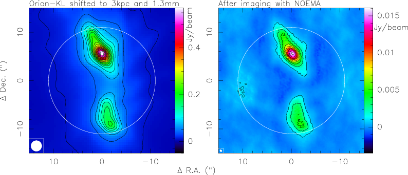
Figure 14: Simulated CORE observations at 1.3 mm wavelength using original data obtained for Orion-KL by Lane et al. (2016). For details of the simulations see appendix A. The beam for the left panel (Orion shifted to 3 kpc) is $2.19^{\prime\prime}$, whereas the synthesized beam of the simulated image in the right panel is $0.44^{\prime\prime}\times 0.34^{\prime\prime}$ (P.A. 44 deg). The contours in the left panel start at 10 mJy beam^-1 and continue in 30 mJy beam^-1 steps. The contours in the right image start at $3\sigma$ and continue in $6\sigma$ steps ($1\sigma\sim 0.3$ mJy beam^-1). The large circles are of $22^{\prime\prime}$ diameter marking the FWHM of the primary beam.

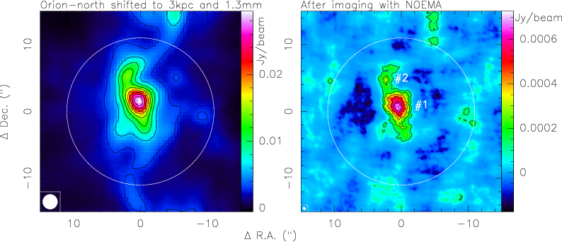
Figure 15: Simulated CORE observations at 1.3 mm wavelength using original data obtained for a field in the northern filament of Orion A by Lane et al. (2016). For details of the simulations see appendix A. The beam for the left panel (Orion shifted to 3 kpc) is $2.19^{\prime\prime}$, whereas the synthesized beam of the simulated image in the right panel is $0.44^{\prime\prime}\times 0.34^{\prime\prime}$ (P.A. 44 deg). The contours in the left panel are in 3 mJy beam^-1 steps. The contours in the right image start are in $3\sigma$ steps ($1\sigma\sim 0.04$ mJy beam^-1). The large circles are of $22^{\prime\prime}$ diameter marking the FWHM of the primary beam.

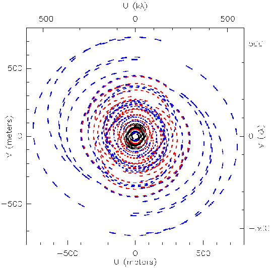
Figure 16: Simulated uv-coverage.

To get a better quantitative understanding on how much the imaging and spatial filtering of the interferometer affects our results, we simulated CORE observations using a distance-scaled bolometer dataset from the Orion molecular cloud. The original Orion 850 $\mu$m data are the large-scale SCUBA-2 observations of Orion A by Lane et al. (2016).

For the simulations, several steps had to be applied to this original dataset. (i) Since our CORE data are at 1.3 mm wavelength, we scaled the flux densities $S$ of the SCUBA-2 850 $\mu$m data by a typical spectral index at (sub)mm wavelength of $S\propto\nu^{3.5}$. (ii) We adapted the intrinsic spatial resolution of the data from the 450 pc distance of Orion (Lane et al., 2016) to 3 kpc (the typical distance of the CORE sample). This implied that the flux densities decrease by $S\propto\left(\frac{450}{3000}\right)^{2}$. (iii) The angular resolution of the original SCUBA-2 data of $14.6^{\prime\prime}$ corresponds at the given distance of 450 pc to a linear resolution of 6570 AU. To maintain the same linear resolution at 3 kpc distance, we changed the pixel size of the image accordingly (from $3^{\prime\prime}$ to $0.45^{\prime\prime}$ pixel size). (iv) Furthermore, we converted the units of the image from mJy arcsec^-2 to mJy beam^-1 and then to K.

From the originally large Orion A image, we selected two sub-regions as examples: (a) a very strong region (Orion-KL), and (b) a fragmented weaker core within the northern part of the integral shape filament (refered to as “Orion-north” in the remaining part of the section). These two files are our model images that are run through the NOEMA simulator as described below. The two model images in units of mJy beam^-1 are shown in Figures 14 and 15 (left panels).

Table 6: Simulation parameters

	Orion-KL	Orion-north
rms (mJy beam-1)	0.3	0.04
rms (mK)	49.8	6.6
$3\sigma\leavevmode\nobreak\ N_{\rm{H_{2}}}$ sensitivity @50 K (cm-2)	$1.5\times 10^{23}$	$1.9\times 10^{22}$
$3\sigma\leavevmode\nobreak\ m_{\rm{H_{2}}}$ sensitivity @50 K (M⊙)	0.1	0.01
missing flux (%)	55	72
$S_{\rm{peak}}(\#1)$ (mJy beam-1)		0.73
$S_{\rm{int}}(\#1)$ (mJy)		40
$S_{\rm{int}}(\#1)$-model (mJy)		99
$S_{\rm{peak}}(\#2)$ (mJy beam-1)		0.3
$S_{\rm{int}}(\#2)$ (mJy)		10
$S_{\rm{int}}(\#2)$-model (mJy)		28

The actual NOEMA simulations were then conducted within the gildas package. As a first step, a representative uv-coverage has to be created within the ASTRO-sub-package by the command uv_tracks. To emulate our simulations best, we used a setup employing the D, B and A-configurations. In each configuration the source was visited 15 times for a length of 15 min each with separations of 40 min between the visits. As target coordinates we used W3(H₂O) (Table 1). The resulting uv-coverage is shown in Fig. 16.

Finally, the visibilities are produced within the gildas sub-package MAPPING and the task uv_fmodel using the above described model images (converted to K) and the given uv-coverage. The resulting visibility data files can then be imaged in exactly the same way as our original CORE data described in section 4. The synthesized beam of the simulated data is $0.44^{\prime\prime}\times 0.34^{\prime\prime}$ (P.A. 44 deg).

As for the original CORE data, the rms varies corresponding to the side-lobes produced by the strongest sources in the field. In the strong Orion-KL field, the rms is 0.3 mJy beam^-1 whereas it is almost an order of magnitude lower (0.04 mJy beam^-1) in the weaker Orion-north field. For details of the simulation parameters see Table 6.

Quantitatively, we extracted the fluxes toward the two main sources (#1 and #2) in Orion-north (Fig. 15, Table 6). Assuming optically thin dust emission at mm wavelengths with an assumed dust temperature of 50 K, we can calculate the corresponding core masses as in the main part of the paper (section 5). The approximate core masses of sources #1 and #2 in Orion-north are then 10.6 and 3.0 M_⊙, respectively. In the Orion-north field itself with the lower rms, we detect both sources well, however, with reduced integrated fluxes at 35 to 40% of the model fluxes (Table 6). Hence, the core masses are underestimated by the same factor. The situation would be different if these two sources were in the same field as Orion-KL. With an rms of 0.3 mJy beam^-1 in the Orion-KL simulation, the peak flux densities of sources #1 and #2 of 0.73 and 0.3 mJy beam^-1 are not above the $3\sigma$ thresholds.

If these Orion-north sources are typical for star-forming regions, then in fields with strong main sources, sub-sources of up $\sim$10 M_⊙ could be difficult to detect. In contrast to that, in fields with weaker main sources, our core mass sensitivity should extend down to 1 M_⊙ or even lower. Therefore, our core-mass sensitivity within the CORE survey is dynamic-range and source-structure limited, and depends on the strongest source in the field. While for weaker sources like Orion-north, we reach almost the thermal noise limit, for stronger sources like Orion-KL, the dynamic range limit of these simulations is $\sim$53.

It should be noted that the above derived core mass sensitivity strongly depends on the size of the cores and hence how much we resolve them. As shown in Table 6, the point source mass sensitivity in both simulations is much smaller at 0.1 and 0.01 M_⊙, respectively. However, this is only valid for point sources. If our model cores were much more compact and all flux within a single synthesized beam, we could easily detect them. But since we know from the original Orion observations their actual sizes, the emission extends over many beams which reduces the mass sensitivity for extended objects significantly.

If we now compare these simulations to the actual range of identified core masses in the survey (Fig. 8), we find that most cores have masses between $\sim$0.2 and 6 M_⊙, below the regime estimated from our simulations. This difference can on the one hand be attributed to the missing flux implying that the core masses themselves are underestimated. But on the other hand, the source structure may also be different in our target regions compared to the Orion data used in these simulations. Beuther et al. (2015) have compared three different starless regions from the low-mass B68 to the intermediate-mass IRDC 19175 and the high-mass IRDC 18310-4 region. They found that the average densities between these three regions varied between $10^{4}$ cm^-3 for the low-mass case to $10^{6}$ cm^-3 for the high-mass region. While the Orion-north region within the integral-shape filament forms rather low- to intermediate-mass stars (in contrast to the high-mass region Orion-KL), our sample is selected to form high-mass stars. Hence, higher densities and more compact structures are expected for the CORE sample. As outlined above, such compact structures make detections of lower-mass objects easier than if the emission is distributed over larger areas. Such structural differences may partly explain the differences between the simulated mass sensitivities and the observed ones.

Appendix B Individual continuum images

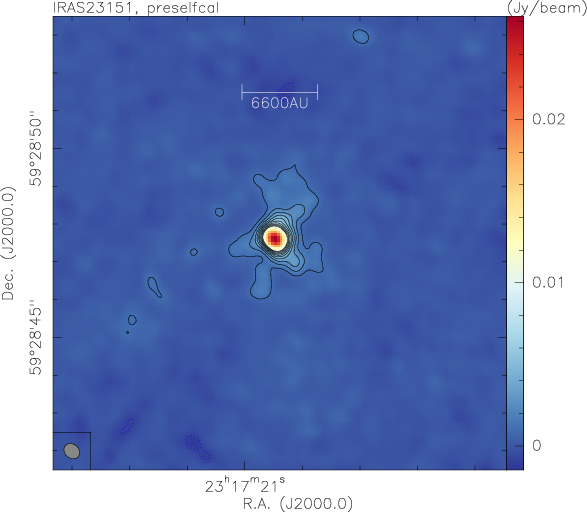
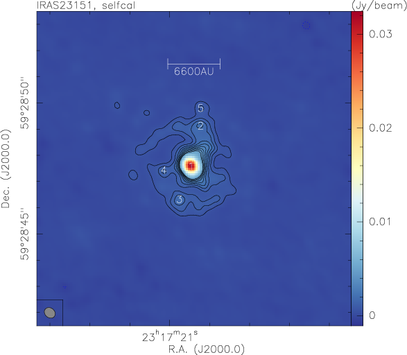
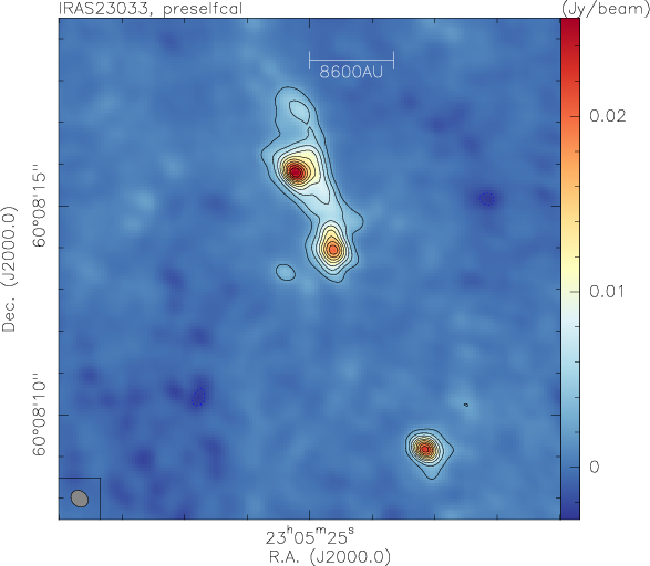
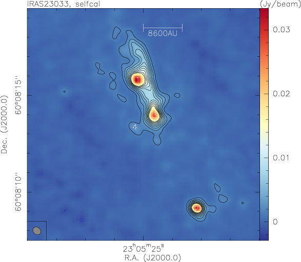
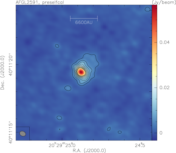
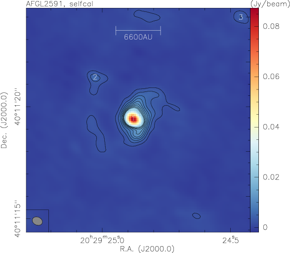
Figure 17: 1.37 mm continuum data for CORE sources. The left panels always show the data without applying self-calibration, and the right panels show them after applying self-calibration. The contours are always in 5$\sigma$ steps (see table 3). The right panels mark the cores identified with clumpfind.

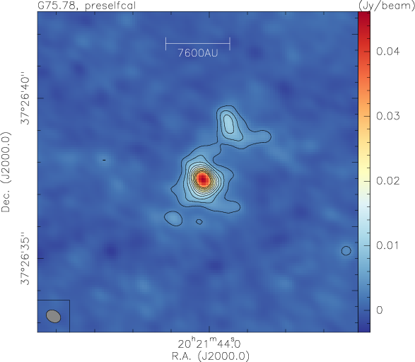
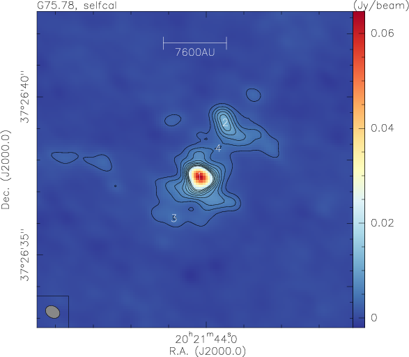
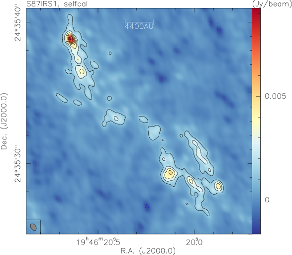
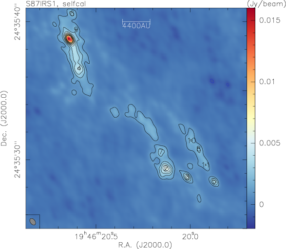
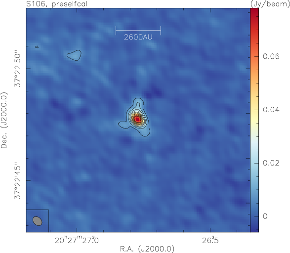
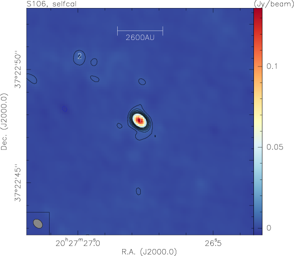
Figure 18: 1.37 mm continuum data for CORE sources. The left panels always show the data without applying self-calibration, and the right panels show them after applying self-calibration. The contours are always in 5$\sigma$ steps (see table 3). The right panels mark the cores identified with clumpfind.

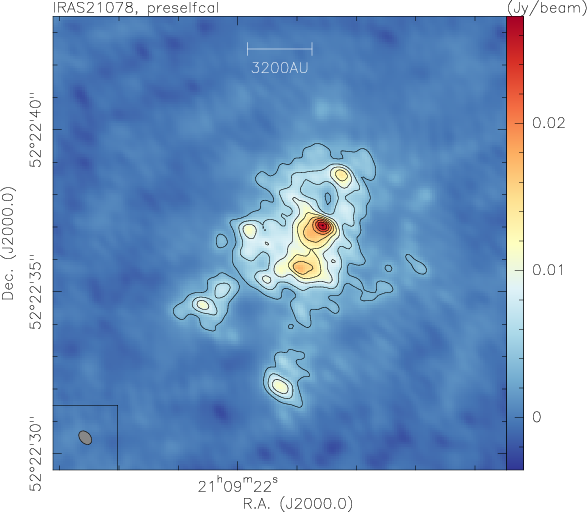
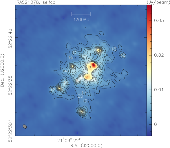
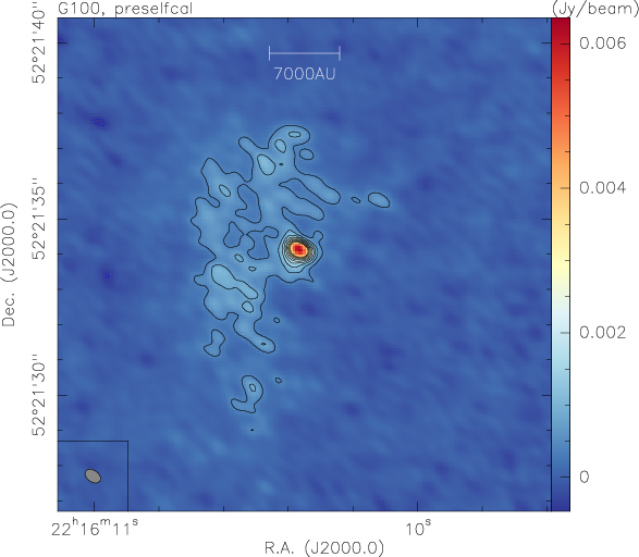
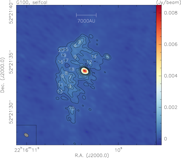
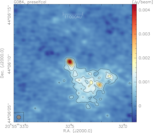
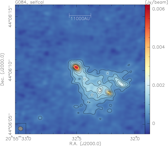
Figure 19: 1.37 mm continuum data for CORE sources. The left panels always show the data without applying self-calibration, and the right panels show them after applying self-calibration. The contours are always in 5$\sigma$ steps (see table 3). The right panels mark the cores identified with clumpfind.

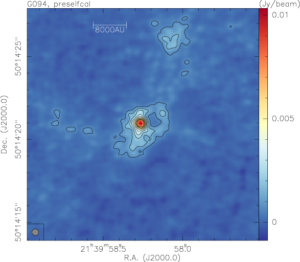
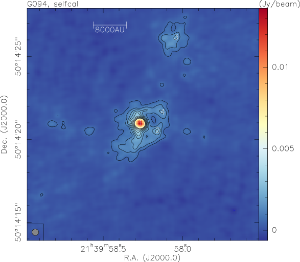
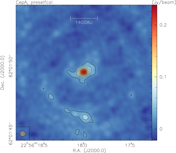
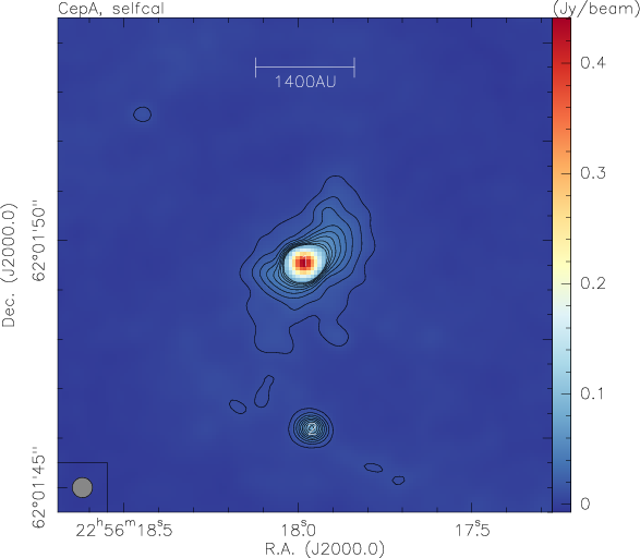
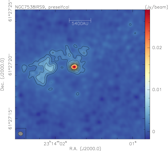
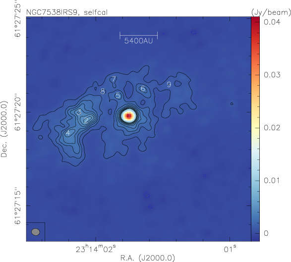
Figure 20: 1.37 mm continuum data for CORE sources. The left panels always show the data without applying self-calibration, and the right panels show them after applying self-calibration. The contours are always in 5$\sigma$ steps (see table 3). The right panels mark the cores identified with clumpfind.

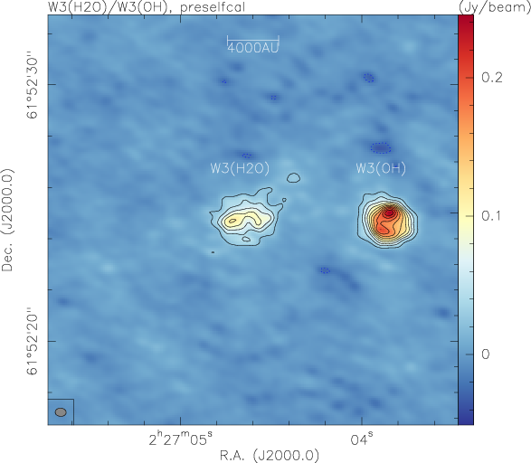
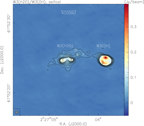
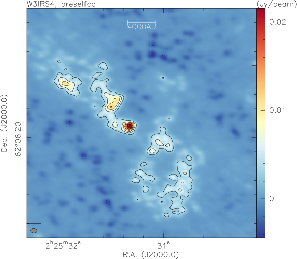
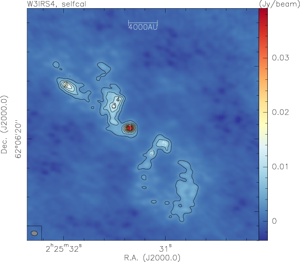
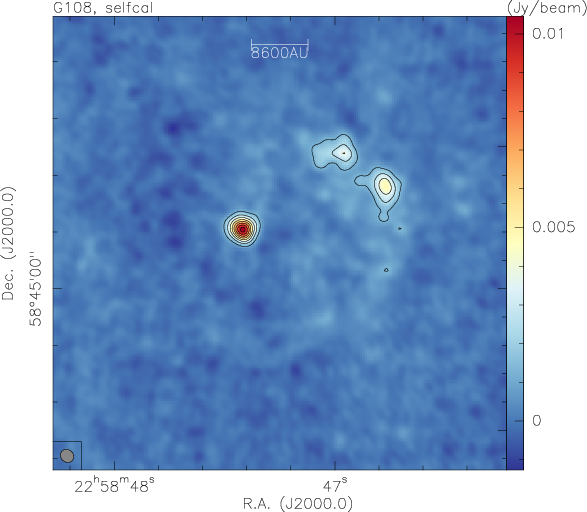
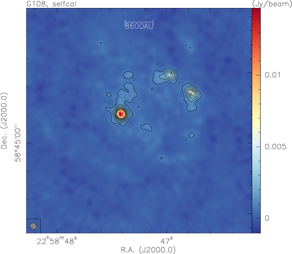
Figure 21: 1.37 mm continuum data for CORE sources. The left panels always show the data without applying self-calibration, and the right panels show them after applying self-calibration. The contours are always in 5$\sigma$ steps (see table 3). The right panels mark the cores identified with clumpfind.

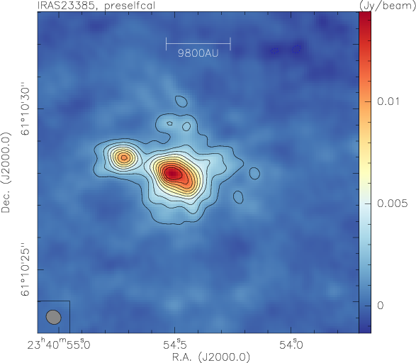
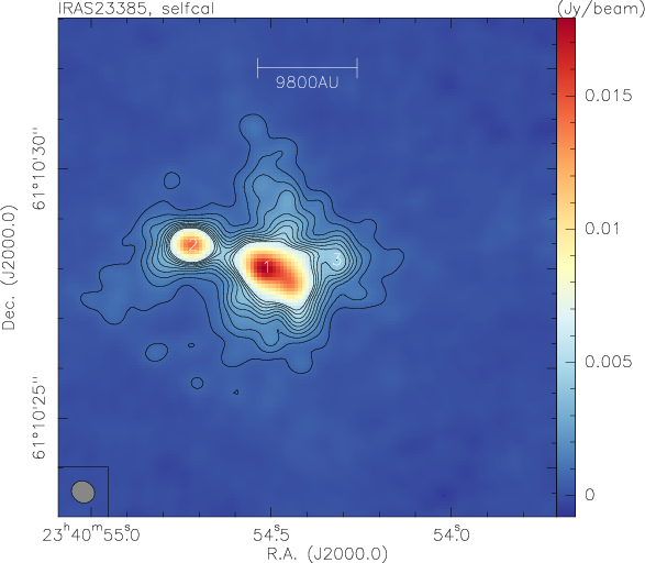
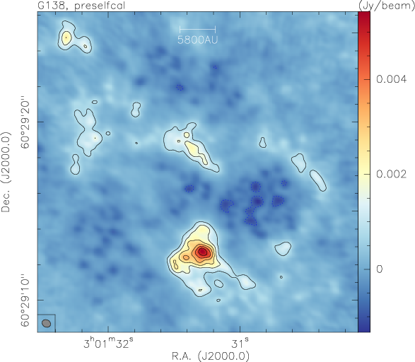
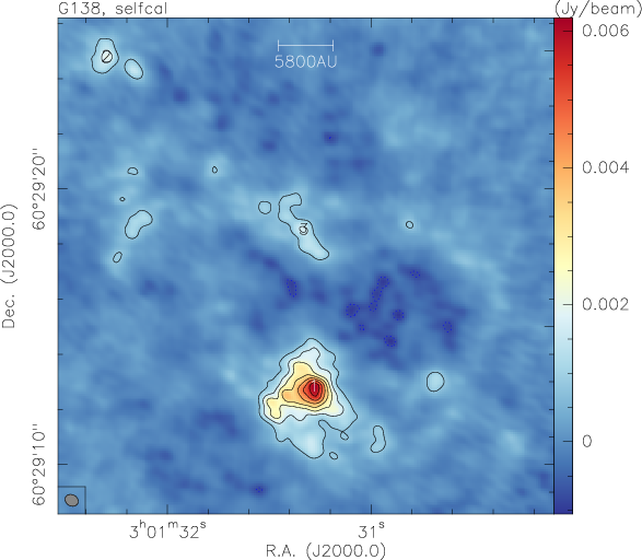
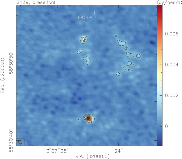
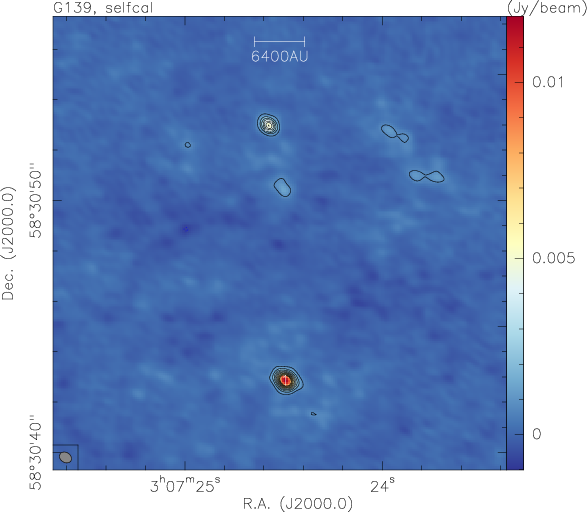
Figure 22: 1.37 mm continuum data for CORE sources. The left panels always show the data without applying self-calibration, and the right panels show them after applying self-calibration. The contours are always in 5$\sigma$ steps (see table 3). The right panels mark the cores identified with clumpfind.

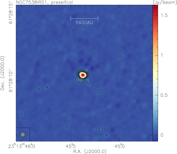
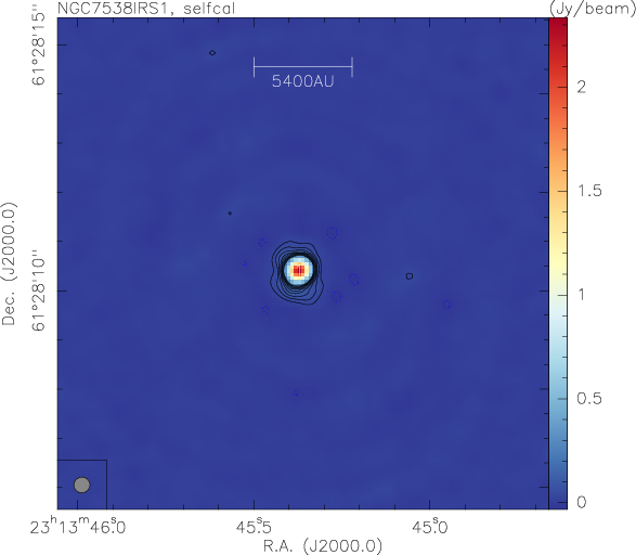
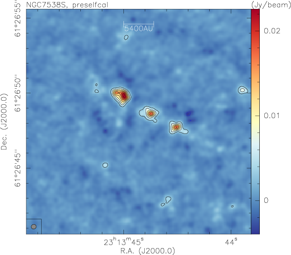
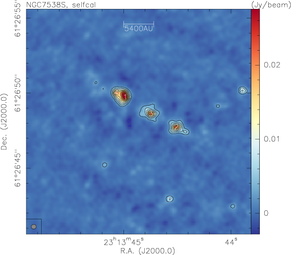
Figure 23: 1.37 mm continuum data for two CORE pilot sources. The left panels always show the data without applying self-calibration, and the right panels show them after applying self-calibration. The contours are always in 5$\sigma$ steps (see table 3). The right panels mark the cores identified with clumpfind.