Found Graph Data and Planted Vertex Covers

Abstract.

A typical way in which network data is recorded is to measure all the interactions among a specified set of core nodes; this produces a graph containing this core together with a potentially larger set of fringe nodes that have links to the core. Interactions between pairs of nodes in the fringe, however, are not recorded by this process, and hence not present in the resulting graph data. For example, a phone service provider may only have records of calls in which at least one of the participants is a customer; this can include calls between a customer and a non-customer, but not between pairs of non-customers.

Knowledge of which nodes belong to the core is an important piece of metadata that is crucial for interpreting the network dataset. But in many cases, this metadata is not available, either because it has been lost due to difficulties in data provenance, or because the network consists of “found data” obtained in settings such as counter-surveillance. This leads to a natural algorithmic problem, namely the recovery of the core set. Since the core set forms a vertex cover of the graph, we essentially have a planted vertex cover problem, but with an arbitrary underlying graph. We develop a theoretical framework for analyzing this planted vertex cover problem, based on results in the theory of fixed-parameter tractability, together with algorithms for recovering the core. Our algorithms are fast, simple to implement, and out-perform several methods based on network core-periphery structure on various real-world datasets.

1. Partially measured graphs, data provenance, and planted structure

Datasets that take the form of graphs are ubiquitous throughout the sciences [4, 27, 54], but the graph data that we work with is generally incomplete in certain systematic ways [33, 38, 39, 41, 44]. Perhaps the most ubiquitous type of incompleteness comes from the way in which graph data is generally measured: we observe a set of nodes $C$ and record all the interactions that they are involved in. The result is a measured graph $G$ consisting of this core set $C$ together with a a potentially larger set of additional fringe nodes — the nodes outside of $C$ that some node in $C$ interacts with. For example, in constructing a social network dataset, we might study the employees of a company and record all of their friendships [59]; from this information, we now have a graph that contains all the employees together with all of their friends, including friends who do not work for the company. This latter group constitutes the set of fringe nodes in the graph. The edge set of the graph $G$ reflects this construction process: we can see all the edges that involve a core node, but if two nodes that both belong to the additional fringe set have interacted, it is invisible to us and hence not recorded in the data.

E-mail and other communication datasets typically look like this; for example, the widely-studied Enron email graph  [28, 42, 48, 60] contains tens of thousands of nodes; however, this graph was constructed from the email inboxes of fewer than 150 employees [40]. The vast majority of the nodes in the graph, therefore, belong to the fringe, and their direct communications are not part of the data. The issue comes up in much larger network datasets as well. For example, a telephone service provider has data on calls and messages that its customers make both to each other and to non-customers; but it does not have data on communication between pairs of non-customers. A massive social network may get some information about the contacts of its users with a fringe set consisting of people who are not on the system — often including entire countries that do not participate in the platform — but generally not about the interactions taking place in this fringe set. And Internet measurements at the IP-layer of service providers provide only a partial view of the Internet for similar reasons [64].

This then is the form that much of our graph data takes (depicted schematically in Figure 1(a)): the nodes are divided into a core set and a fringe set, and we only see the edges that involve a member of the core set. This means, in particular, that the core set is a vertex cover of the underlying graph — since a vertex cover, by definition, is a set that is incident to all the edges.

 

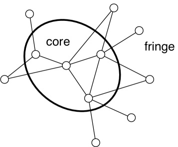
(a) Graph data built from a small core

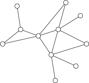
(b) The dataset without the core labeled

Figure 1. (a) Graph datasets are often constructed by recording all the interactions involving a set of measured core nodes; the resulting data contains these core nodes together with a potentially much larger fringe, consisting of all other nodes that had an interaction with some member of the core. We can see the links between members of the fringe and members of the core, but links between pairs of nodes in the fringe are not recorded and hence not visible in the data. (b) It is important for interpreting the dataset that the metadata describing which nodes belong to the core be preserved. But in many cases, this metadata is not available — either because of challenges in data provenance that lead to the loss of the metadata, or because the graph is “found data” obtained in a context such as counter-surveillance. The challenge is then to determine how accurately we can recover the core, despite limited information about how the dataset was constructed. Algorithmically, this leads to a planted vertex cover problem, in which we are given a graph and are tasked with identifying a hidden vertex cover (the core).

In many cases, a graph dataset comes annotated with metadata about which nodes belong to the core, and this is crucial for correctly interpreting the data. But there are a number of important contexts where this metadata is not available, and we simply do not know which nodes constitute the core. In other words, at some point, we have “found data” that we know has a core, but the labels are missing. One reason for this scenario is that over time, metadata becomes lost for a wide range of reasons; this is a central underlying theme in data provenance, lineage, and preservation [12, 49, 61, 63], and an issue that has become especially challenging with modern efforts in digitization [43] and the increasing size of data management efforts [37]. For example, data is repeatedly shared and manipulated, URLs become defunct, managers of datasets change jobs, and hard drives are decommissioned. Natural scenarios embodying these forces proliferate; consider for example an anonymized research dataset of telephone call records, shared between a telecommunications company and a university, which did not include metadata on which nodes were the customers and which were the fringe set of non-customers. By the time the graduate student doing research on the dataset comes to know that this metadata is missing and important for analysis, the researchers at the company who originally assembled the dataset have left, and there is no easy way to reconstruct the metadata.

These issues arise in very similar forms in current research on the process of counter-surveillance [34]. Intelligence agencies may intercept data from adversaries conducting surveillance and build a graph to determine which communications the adversaries were recording. In different settings, activist groups may petition for the release of surveillance data by governments, or infer it from other sources [52]. In all these cases, the “found data” consists of a communication graph in which an unknown core subset of the nodes was observed, and the remainder of the nodes in the graph (the fringe) are there simply because they communicated with someone in the core. But there may generally not be any annotation in such situations to distinguish the core from the fringe. In this case, the core nodes are the compromised ones, and identifying the core from the data can help to warn the vulnerable parties, hide future communications, or even disseminate misinformation.

Planted Vertex Covers.

Here we study the problem of recovering the set of core nodes in found graph data, motivated by this range of settings in which reconstructing an unknown core is a central question. Algorithmically, the problem can be stated simply as a planted vertex cover problem: we are given a graph $G$ in which an adversary knows a specific vertex cover $C$; we do not know the identity of $C$, but our goal is to output a set that is as close to $C$ as possible. Here, the property of being “close” to $C$ corresponds to a performance guarantee that we will formulate in several different ways: we may, for example, want to output a set not much larger than $C$ that is guaranteed to completely contain it; or we may want to output a small set that is guaranteed to have significant overlap with $C$. A simple instance of the task is depicted in Figure 1(b), after the explicit labeling of the core nodes has been removed from Figure 1(a).

Planted problems have become an active topic of study in recent years. Generically they correspond to a style of problem in which some hidden structure (like the vertex cover in our case) has been “planted” in a larger input, and the goal is to find the structure in the given input. Planted problems tend to be based on formal frameworks in which the input is generated by a highly structured probabilistic model. Perhaps the two most heavily-studied instances are the planted clique problem [5, 24, 29, 51], in which a large clique is added to an Erdős-Rényi random graph; and the recovery problem for stochastic block models [1, 2, 3, 7, 23, 53], in which a graph’s edges are generated independently at random, but with higher density inside communities than between.

It might seem essentially inevitable that planted problems should require such strong probabilistic assumptions — after all, how else could an algorithm possibly guess which part of the graph corresponds to the planted structure, if there are no assumptions on what the “non-planted” part of the graph looks like?

But the vertex cover problem turns out to be different, and it makes it possible to solve what, surprisingly, can be described as a kind of “worst-case” planted problem — with extremely limited assumptions, it is possible to design algorithms capable of finding sets that are close to unknown vertex covers in arbitrary graphs. Specifically, we make only two assumptions about the input (both of them necessary in some form, though relaxable): that the planted vertex cover is inclusionwise minimal, and that its size is upper-bounded by a known quantity $k$. It is natural to think of $k$ as relatively small compared to the total number of nodes $n$, in keeping with the fact that in much of the measured graph data, the core is small relative to the fringe. We draw on results from the theory of fixed-parameter tractability to show that there is an algorithm operating on arbitrary graphs that can output a set of $f(k)$ nodes (independent of the size of the graph) that is guaranteed to contain the planted vertex cover. We obtain further results as well, including stronger bounds when the size of the planted vertex cover is close to minimum; when we can partially overlap the planted vertex cover without fully containing it; and when the graph is generated from a natural probabilistic model.

We pair these theoretical guarantees with computational experiments in which we show the effectiveness of these methods on graph datasets exhibiting this structure in practice. Using the ingredients from our theoretical results, we develop a natural heuristic based on unions of minimal vertex covers, each obtained via pruning a 2-approximate maximal matching algorithm for minimum vertex covers with random initialization. The entire algorithm is implemented in just 30 lines of Julia code (see Fig. 3 for the complete implementation). Our algorithm provides superior empirical performance and superior running time across a range of real datasets compared to a number of competitive baseline algorithms. Among these, we show improvements over a line of well-developed heuristics for detecting core-periphery structure in graphs [17, 36, 58, 67] — a sociological notion related to our concerns here, in which a graph has a dense core and a sparser periphery, generally for reasons of differential status rather than measurement effects.

2. Theoretical methodology for partial recovery or tight containment

We begin by formalizing the recovery problem. Suppose there is a large universe of nodes $U$ that interact via communication, friendship, or some other mechanism. We choose a core subset $C\subseteq U$ of these nodes and measure all the pairwise interactions that involve at least one node in $C$. We represent our measurement on $C$ by a graph $G=(V,E)$, where $V\subseteq U$ is all nodes that belong to $C$ or participate in a pairwise link with at least one node in $C$, and $E$ is the set of all such links. The set of nodes in $V-C$ will be called the fringe of the graph. We will ignore directionality and self-loops so that $G$ is a simple, undirected graph. Note that under this construction, $C$ is a vertex cover of $G$.

2.1. Finding a planted vertex cover

Now, suppose we are shown the graph $G$ and are tasked with finding the core $C$. Can we say anything non-trivial in answer to this question? In the absence of any other information, it could be that $C=V$, so we first make the assumption that we are given a bound $k$ on the size of $C$, where we think of $k$ as small relative to the size of $V$. With this extra piece of information, we can ask if it is possible to obtain a small set that is guaranteed to contain $C$. We state this formally as follows.

Question 1.

For some function $f$, can we find a set $D$ of size at most $f(k)$ (independent of the size of $V$) that is guaranteed to contain the planted vertex cover $C$?

The answer to this question is “no”. For example, let $k=2$ and let $G$ be a star graph with $n>3$ nodes $v_{1},...,v_{n}$ and edges $(v_{1},v_{i})$ for each $i>1$. The two endpoints of any edge in the graph form a vertex cover of size $k=2$, but $C$ could conceivably be any edge. Thus, under these constraints, the only set guaranteed to contain $C$ is the entire node set $V$.

This negative example uses the fact that once we put $v_{1}$ into a 2-node vertex cover for the star graph, the other node can be arbitrary, since it is superfluous. The example thus suggests that a much more reasonable version of the question is to ask about minimal vertex covers; formally, $C$ is a minimal vertex cover if for all $v\in C$, the set $C-\{v\}$ is not a vertex cover. (We contrast this with the notion of a minimum vertex cover — a definition we also use below — which is a vertex cover whose size is minimum among all vertex covers for the given graph.) Minimality is a natural definition with respect to our original motivating application as well, where it would be reasonable to assume that the set of measured nodes was non-redundant, in the sense that omitting a node from $C$ would cause at least one edge to be lost from the measured communication pattern. This would imply that $C$ is a minimal vertex cover. With this in mind, we ask the following adaptation of Question 1:

Question 2.

If $C$ is a minimal planted vertex cover, can we find a set $D$ of size at most $f(k)$ (independent of $\lvert V\rvert$) that is guaranteed to contain $C$?

Interestingly, the answer to this question is “yes,” for arbitrary graphs. We derive this as a consequence of a result due to Damaschke [19, 20] in the theory of fixed-parameter tractability. While this theory is generally motivated by the design of fast algorithms, it is also a source of important structural results about graphs. The structural result we use here is the following.

Lemma 1 ([19, 20]).

Consider a graph $G$ with a minimum vertex cover size $k^{*}$. Let $U(k)$ be the union of all minimal vertex covers of size at most $k$. Then

• $\lvert U(k)\rvert\leq(k+1)^{2}/4+k$ and is asymptotically tight [19, Theorem 3]

• $\lvert U(k)\rvert\leq(k-k^{*}+2)k^{*}$ and is tight [20, Theorem 12]

For part (a) of this lemma, there is an appealingly direct proof that gives the $O(k^{2})$ asymptotic bound, using the following kernalization technique from the theory of fixed-parameter tractability [14, 25]. The proof begins from the following observation:

Observation 1.

Any node with degree strictly greater than $\lvert C\rvert$ must be in $C$.

The observation follows simply from the fact that if a node is omitted from $C$, then all of its neighbors must belong to $C$. Thus, if $S$ is the set of all nodes in $G$ with degree greater than $k$, then $S$ is contained in every vertex cover of size at most $k$; hence Observation 1 implies that if $U(k)$ is non-empty, we must have $|S|\leq k$ and $S\subseteq U(k)$. Now $G-S$ is a graph with maximum degree $k$ and a vertex cover of size $\leq k$, so it has at most $O(k^{2})$ edges; let $T$ be the set of all nodes incident to at least one of these edges. Any node not in $S\cup T$ is isolated in $G-S$ and hence not part of any minimal vertex cover of size $\leq k$; therefore $U(k)\subseteq S\cup T$, and so $|U(k)|=O(k^{2})$.

The following theorem, giving a positive answer to Question 2, is thus a corollary of Lemma 1(a) obtained by setting $D=U(k)$.

Theorem 1.

If $C$ is a minimal planted vertex cover with $\lvert C\rvert\leq k$, then we can find a set $D$ of size $O(k^{2})$ that is guaranteed to contain $C$.

To see why $O(k^{2})$ is a tight bound, consider a graph $G$ consisting of the disjoint union of $k/2$ stars each with $1+k/2$ leaves. Any set consisting of the centers of all but one of the stars, and the leaves of the remaining star, is a minimal vertex cover of size $k$. But this means that every node in $G$ could potentially belong to the planted vertex cover $C$, and so the only acceptable answer is to output the full node set $V$. Since $V$ has size $\Omega(k^{2})$, the bound follows.

There are algorithms to compute $U(k)$ that run in time exponential in $k$ but polynomial in the number of nodes for fixed $k$ [20]. For the datasets we consider in this paper, these algorithms are impractical, despite the polynomial dependence on the number of nodes. However, we will use the results in this section as the basic ingredients for an algorithm, developed in Section 3, that works extremely well in practice.

2.2. Non-minimal vertex covers

A natural next question is whether we can say anything positive when the planted vertex cover $C$ is not minimal. In particular, if $C$ is not minimal, can we still ensure that some parts of it must be contained in $U(\lvert C\rvert)$? The following propositions show that if a node $u\in C$ links to a node $v$ that is outside $C$, or that is deeply contained in $C$ (with $v$ and its neighbors all in $C$), then $u$ must belong to $U(\lvert C\rvert)$.

Proposition 1.

If $u\in C$ and there is an edge $(u,v)$ to a fringe node $v\notin C$, then $u\in U(\lvert C\rvert)$.

Proof.

Consider the following iterative procedure for “pruning” the set $C$: we repeatedly check whether there is a node $w$ such that $C-\{w\}$ is still a vertex cover; and if so, we choose such a $w$ and delete it from $C$. When this process terminates, we have a minimal vertex cover $C^{\prime}\subseteq C$; and since $|C^{\prime}|\leq\lvert C\rvert$, we must have $C^{\prime}\subseteq U(\lvert C\rvert)$. But in this iterative process we cannot delete $u$, since $(u,v)$ is an edge and $v\not\in C$. Thus $u\in C^{\prime}$, and hence $u\in U(\lvert C\rvert)$. ∎

Next, let us say that a node $v$ belongs to the interior of the vertex cover $C$ if $v$ and all the neighbors of $v$ belong to $C$. We now have the following result.

Proposition 2.

If $u\in C$ and there is an edge $(u,v)$ to a node $v$ in the interior of $C$, then $u\in U(\lvert C\rvert)$.

Proof.

Let $u$ and $v$ be nodes as described in the statement of the proposition. Since all of $v$’s neighbors are in $C$, it follows that $C_{0}=C-\{v\}$ is a vertex cover. We now proceed as in the previous proof: we iteratively delete nodes from $C_{0}$ as long as we can preserve the vertex cover property. When this process terminates, we have a minimal vertex cover $C^{\prime}\subseteq C_{0}$, and since $|C^{\prime}|\leq\lvert C\rvert$, we must have $C^{\prime}\subseteq U(\lvert C\rvert)$. Now, $u$ could not have been deleted during this process, because $(u,v)$ is an edge and $v\not\in C_{0}$. Thus $u\in C^{\prime}$, and hence $u\in U(\lvert C\rvert)$. ∎

Even with these results, we can find instances where an arbitrarily small fraction of the nodes in a non-minimal planted vertex cover $C$ may be contained in $U(\lvert C\rvert)$. To see this, consider a star with center node $u$ and $k+1$ leaves; and let $C$ consist of $u$ together with any $k-1$ of the leaves. We observe that the single-node set $\{u\}$ is the only minimal vertex cover of size at most $k$, and hence $\lvert U(\lvert C\rvert)\rvert/\lvert C\rvert=1/k$. Note how in this example, all the other nodes of $C$ fail to satisfy the hypotheses of Proposition 1 or 2. However, we will see in Section 3 that in all of the real-world network settings we consider, these three propositions can be used to show that most of $C$ is indeed contained in $U(\lvert C\rvert)$.

Our bad example consisting of a star also has the property that the planted vertex $C$ is much larger than the size of a minimum vertex cover. We next consider the case in which $C$ may be non-minimal, but is within a constant multiplicative factor of this minimum size $k^{*}$. In this case, we will show how to find small sets guaranteed to intersect a constant fraction of the nodes in $C$.

2.3. Maximal matching 2-approximation to minimum vertex cover and intersecting the core

Input: Graph $G=(V,E)$

Output: Vertex cover $M$ with $\lvert M\rvert\leq 2k^{*}$

$M\leftarrow\varnothing$

for $e=(u,v)\in E$ do

       if $u\notin M$ and $v\notin M$ then $M\leftarrow M\cup\{u,v\}$

      

Algorithm 1 Maximal matching 2-approximation for minimum vertex cover

A basic building block for our theory in this section and the algorithms we develop later is the classic maximal matching 2-approximation to minimum vertex cover (Algorithm 1, above). The algorithm greedily builds a maximal matching $M$ by processing each edge $e=(u,v)$ of the graph and adding $u$ and $v$ to $M$ if neither endpoint is already in $M$. Upon termination, $M$ is both a maximal matching and a vertex cover: it is maximal because if we could add another edge $e$, then it would have been added when we processed edge $e$; and it is a vertex cover because if both endpoints of an edge $e$ are not in the matching, then $e$ would have been added to the matching when it was processed. Since any vertex cover must contain at least one endpoint from each edge in the matching, we have $k^{*}\geq\lvert M\rvert/2$; or, equivalently, $\lvert M\rvert\leq 2k^{*}$, where $k^{*}$ is the minimum vertex cover size of $G$. We note that the output $M$ of Algorithm 1 may not be a minimal vertex cover. However, we can iteratively prune nodes from $M$ to make it minimal, which we will do for our recovery algorithm described in Section 3. For the theory in this section, though, we assume no such pruning.

The following proposition shows that any vertex cover whose size is bounded by a constant multiplicative factor of the minimum vertex cover size must intersect the output of Algorithm 1 in a constant fraction of its nodes.

Lemma 2.

Let $B$ be any vertex cover of size $\lvert B\rvert\leq bk^{*}$ for some constant $b$. Then any set $M$ produced by Algorithm 1 satisfies $\lvert M\cap B\rvert\geq\frac{1}{2b}\lvert B\rvert$.

Proof.

The maximal matching consists of $h$ edges satisfying $h=|M|/2\leq k^{*}$. Since $B$ is a vertex cover, it must contain at least one endpoint of each of the $h$ edges in $M$. Hence, $\lvert M\cap B\rvert\geq h\geq k^{*}/2\geq\frac{1}{2b}\lvert B\rvert$. ∎

A corollary is that if our planted cover $C$ is relatively small in the sense that it is close to the minimum vertex cover size, then Algorithm 1 must partially recover $C$. We write this as follows.

Corollary 1.

If the planted vertex cover $C$ has size $\lvert C\rvert\leq ck^{*}$, then Algorithm 1 produces a set $M$ of size $\leq 2k^{*}$ that intersects at least a $1/(2c)$ fraction of the nodes in $C$.

An important property of Algorithm 1 that will be useful for our algorithm design later in the paper is that the algorithm’s guarantees hold regardless of the order in which the edges are processed. Furthermore, two matchings produced by the algorithm using two different orderings of the edges must share a constant fraction of nodes, as formalized in the following corollary.

Corollary 2.

Any two sets $S_{1}$ and $S_{2}$ obtained from Algorithm 1 (with possible different orders in the processing of the edges) satisfy $\lvert S_{1}\cap S_{2}\rvert\geq\frac{1}{4}\max(\lvert S_{1}\rvert,\lvert S_{2}\rvert)$.

Thus far, everything has applied without any assumptions on the graph itself, other than the fact that it contains a vertex cover of size at most $k$. In the following section, we show how different ways of assuming structure on the graph can yield stronger guarantees.

2.4. Improving results with known graph structure

We now examine ways to strengthen our theoretical guarantees by assuming some structure on $C$ and $G$. For a simple example, if $C$ induces a clique in $G$, then the subgraph on $C$ has a minimum vertex cover of size $\lvert C\rvert-1$; in this case the second bound in Lemma 1 reduces to $\lvert U(\lvert C\rvert)\rvert\leq 3\lvert C\rvert$. Furthermore, in this case, Observation 1 would say that any node in $C$ that has an edge to a fringe node outside of $C$ is immediately identifiable from its degree (if we knew the size of $C$). Below, we consider how to make use of random structure or bounds on the minimum vertex cover size $k^{*}$ obtained through computation with Algorithm 1 to strengthen our theoretical guarantees.

Stochastic block model. One common structural assumption is that edges are generated independently at random. The stochastic block model (SBM) is a common generative model for this idealized setting [35]. In our case, we use a 2-block SBM, where one block is the planted vertex cover $C$ and the other block is the remaining fringe nodes $F=V-C$. The SBM provides a single probability of an edge forming within a block and between blocks. For our purposes, $C$ is a vertex cover, so we assume that the probability of an edge between nodes in $F$ is 0. For notation, we will say that the probability of an edge between nodes in $C$ is $p$ and the probability of an edge between a node in $C$ and a node in $F$ is $q$. We make no assumption on the relative values of $p$ and $q$. SBMs have previously been used to model core-periphery structures in networks [67], although this prior work assumes that $p>q$ and that there is a probability $r<q$ of nodes in the periphery forming an edge. (In Section 3, we compare against the belief propagation algorithm developed in this prior work.)

Our technical result here combines the second bound in Lemma 1 with the well-known lower bounds on independent set size in Erdős-Rényi graphs (in the SBM, $C$ is an Erdős-Rényi graph with edge probability $p$).

Lemma 3.

With probability at least $1-\lvert C\rvert^{-3\ln n/(2p)}$), the union of minimal vertex covers of size at most $\lvert C\rvert$ contains at most $\lvert C\rvert(3\ln\lvert C\rvert/p+3)$ nodes.

Proof.

It is straightforward to show that the independence number $\alpha$ of $C$ is less than $(3\ln\lvert C\rvert)/p+1$ with probability at least $1-\lvert C\rvert^{-3\ln\lvert C\rvert/(2p)}$ [62]. The minimum vertex cover size of the first block is then $k^{*}=\lvert C\rvert-\alpha\geq\lvert C\rvert-(3\ln\lvert C\rvert)/p-1$ with the same probability. Plugging into Lemma 1(b) gives the result. ∎

We could improve the constants in the above statement with more technical results on the independence number in Erdős-Rényi graphs [21, 31]. However, our point here is simply that the SBM provides substantial structure. The following theorem further represents this idea.

Theorem 2.

Let $C$ be a planted vertex cover in our SBM model, where we know that $\lvert C\rvert=k$. Let $p$ and $q$ be constants, and let the number of nodes in the stochastic block model be $ck$ for some constant $c\geq 1$. Then with high probability as a function of $k$, there is a set $D$ of size $O(k\log k)$ that is guaranteed to contain $C$.

Proof.

By Lemma 3, we know that $\lvert U(k)\rvert$ is $O(k\log k)$ with high probability. Now, for any node $v\in C$, the probability that it links to at least one node outside of $C$ is $1-(1-q)^{(c-1)k}$. Taking the union bound over all nodes in $C$ shows that with high probability in $k$, each node in $C$ has at least one edge to a node outside $C$. In this case, Proposition 1 implies that $C\subseteq U(k)$, so by computing $U(k)$, we contain $C$ with high probability. ∎

Bounds on the minimum vertex cover size. While it may sometimes be impractical to compute the minimum vertex cover size $k^{*}$, the second bound of Lemma 1 may still be used if we can bound $k^{*}$ from above and below. Specifically, given a lower bound $l$ and an upper bound $u$ on $k^{*}$, $\lvert U(k)\rvert\leq(k-k^{*}+2)k^{*}\leq(k-l+2)u$. Here, we have a scenario in which we want the lower bound $l$ to be as large as possible and the upper bound $u$ to be as small as possible.

A cheap way of finding such bounds is to use the greedy maximal matching approximation algorithm (Algorithm 1). We can run the approximation algorithm $N$ times, processing the edges in different (random) orders, producing sets $S_{1},\ldots,S_{N}$ of sizes $s_{1},\ldots,s_{N}$. We can then set the largest lower bound obtained to be $l=\max_{j}s_{j}/2$. As noted in Section 2.3, the sets $S_{j}$ are not guaranteed to be minimal. We can post-process them to be minimal, producing sets $S^{\prime}_{1},\ldots,S^{\prime}_{N}$ of sizes $s^{\prime}_{1},\ldots,s^{\prime}_{N}$. Setting $u=\min_{j}s^{\prime}_{j}$ gives us the smallest upper bound. Through the lens of this procedure, the search for a large lower bound makes sense. If we can find a lower bound $l$ and an upper bound $u$ such that $l=2u$, then we know that $k^{*}=l$. In other words, larger lower bounds, combined with the 2-approximation, are giving us more information on the interval containing $k^{*}$.

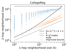
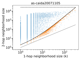
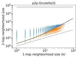
Figure 2. Improvements in the second bound from Lemma 1 by bounding the minimum vertex cover size. The planted vertex covers are 1-hop neighborhoods of a node, which cover the 2-hop neighborhoods (the center node is excluded). Blue dots in the scatter plot show the relative sizes of the planted cover and the total number of vertices in the subgraph. Blue dots above the thick black curve represent non-trivial bounds from the first bound in Lemma 1 (i.e., the size of the union of covers is less than the size of the 2-hop neighborhood itself). The orange squares show improvements in the bound by approximating the minimum vertex cover size. In many cases, this substantially improves the bound. For the CollegeMsg dataset, the bounds appear to be linear instead of quadratic.

Before getting to our main computational results in the next section, we begin by evaluating this particular bounding methodology on three datasets: (i) a network of private messages sent on an online social network at the University of California, Irvine (CollegeMsg; [56]), (ii) an autonomous systems graph derived from a RouteViews BGP table snapshot in November, 2007 (as-caida20071105; [46]), (iii) a snapshot of the Gnutella peer-to-peer file sharing network from August 2002 (p2p-Gnutella31; [50]). For each network, we construct planted covers by considering the 1-hop neighborhood of nodes $u$ as a cover for the 2-hop neighborhood of the same node (and we remove the node $u$ from both of these sets). This provides a collection of planted vertex covers in communication-like datasets. We set $N=20$ and use the above procedure to employ the second bound in Lemma 1 without computing any minimum vertex covers. Figure 2 summarizes the results. We observe that in most cases, the first bound in Lemma 1 is non-trivial (i.e., is smaller than the size of the 2-hop neighborhood) and that the approximations can substantially improve the bound. In the case of the CollegeMsg dataset, the upper bounds appear approximately linear in the cover size.

3. Recovery performance on datasets with “real” planted vertex cores

Table 1. Basic summary statistics of our graph datasets: the number of nodes ($n$), number of edges ($m$), total time spanned by the dataset, size of the planted vertex cover ($\lvert C\rvert$), minimum vertex cover size ($k^{*}$), bounds from Lemma 1 given as a fraction of the total number of nodes (capped at 1, the trivial bound), fraction of nodes in $u\in C$ that are in an edge with $v\notin C$, and fraction of nodes in $C$ with a neighbor $v$ in the interior of $C$ ($v$ and all of its neighbors are in $C$). The nodes in these last two categories are guaranteed to be in the union of all minimal vertex covers of size at most $\lvert C\rvert$ by Propositions 1 and 2. Across all datasets, most nodes in $C$ fall into these categories.

Dataset	n	m	time span	$\lvert C\rvert$	$k^{*}$	Bound 1	Bound 2	frac. $C$ w/	frac. $C$ w/
			(days)					edge outside $C$	interior neighbor
email-Enron	18.6k	43.2k	1.50k	146	146	0.30	0.02	0.99	0.00
email-W3C	20.1k	31.9k	7.52k	1.99k	1.11k	1.00	1.00	0.76	0.06
email-Eu	202k	320k	804	1.22k	1.18k	1.00	0.26	0.99	0.00
call-Reality	9.02k	10.6k	543	90	82	0.24	0.09	0.90	0.01
text-Reality	1.18k	1.95k	478	84	80	1.00	0.41	0.88	0.00

We now study how well we can recover planted vertex covers, where the vertex cover corresponds to a core set arising from the type of measurement process described in the introduction. We use five datasets for this purpose:

1. email-Enron [40]: This is the dataset discussed in the introduction, where the core is the set of email addresses for which the inboxes were released as part of the investigation by the Federal Energy Regulatory Commission. Nodes are email addresses and there is an edge between two addresses if an email was sent between them.

2. email-W3C [16, 55, 65]: This is a dataset of email threads crawled from W3C mailing lists. We consider the “core” to be the nodes with a w3.org domain in the email address. There is an edge between two email addresses if an email was sent between them.

3. email-Eu [47, 66]: This dataset consists of email communication involving members of a European research institution. The core represents the members of the research institution.

4. call-Reality [26]: This dataset consists of phone calls made and received by a set of students and faculty at the MIT Media Laboratory or MIT Sloan business school as part of the reality mining project. These students and faculty constitute the core. There is an edge between any two phone numbers between which a call was made.

5. text-Reality [26]: This dataset has the same core nodes as the phone-Reality dataset but edges are formed via SMS text communications instead of phone calls.

Each dataset has timestamps associated with the nodes, and we will evaluate how well we can recover the core as the networks evolve. Table 1 provides some basic summary statistics of the datasets. The table includes the minimum vertex cover size (computed using Gurobi’s linear integer program solver), which lets us evaluate the second bound of Lemma 1. We also computed the fraction of nodes that are guaranteed to be in $U(\lvert C\rvert)$ by Propositions 1 and 2 and find that 82%–99% of the nodes fit these guarantees, depending on the dataset.

3.1. The union of minimal vertex covers algorithm and recovery performance

We now study how well we can recover the planted vertex cover consisting of the core $C$. All of the methods we use provide an ordering on the nodes, often through some score function on the nodes in the graph. We then evaluate recovery on two criteria: (i) precision at core size (i.e., the fraction of nodes in the top $\lvert C\rvert$ of the ordering that are actually in $C$) and (ii) area under the precision recall curve (this metric is more appropriate than area under the receiver operating characteristic curve when there is class imbalance [22], which is the case here).

⬇

1function UMVC(A::SparseMatrixCSC{Int64,Int64}, ncovers=300)

2 edgevec = filter(e -> e[1] < e[2],

3 collect(zip(findnz(A)[1:2]...)))

4 umvc = zeros(Int64, size(A,1))

5 for _ in 1:ncovers

6 # Run 2-approximation with random edge ordering

7 cover = zeros(Int64, size(A,1))

8 edge_queue = shuffle(edgevec)

9 while length(edge_queue) > 0

10 i, j = pop!(edge_queue)

11 if cover[[i,j]] == [0,0]; cover[[i,j]] = [1,1]; end

12 end

13 # Reduce to a minimal cover

14 while true

15 reduced = false

16 for c in shuffle(find(cover .== 1))

17 nbrs = find(A[:,c])

18 if sum(cover[nbrs]) == length(nbrs)

19 cover[c] = 0

20 reduced = true

21 end

22 end

23 if !reduced; break; end

24 end

25 umvc[cover .== 1] = 1

26 end

27 d = vec(sum(A,2)) # degrees of nodes

28 return [sort(find(umvc .== 1), by=v->d[v], rev=true);

29 sort(find(umvc .== 0), by=v->d[v], rev=true)]

30end

Figure 3. Complete implementation of our union of minimal vertex covers (UMVC) algorithm in 30 lines of Julia code. The algorithm repeatedly runs the standard maximal matching 2-approximation algorithm for minimum vertex cover (Algorithm 1; lines 6–12) and reduces each cover to a minimal one (lines 13–24). The union of covers is ranked first in the ordering (sorted by degree; line 28). The remaining nodes are then sorted by degree (line 29). The code is available as a Gist at https://gist.github.com/arbenson/c1251f0851fdfc97021b9a0a37d4fb69.

Proposed algorithm: union of minimal vertex covers (UMVC). Our proposed algorithm, which we call the union of minimal covers (UMVC), repeatedly finds minimal vertex covers and takes their union. The nodes in this union are ordered by degree and the remaining nodes (not appearing in any minimal core) are ordered by degree. The minimal covers are constructed by first finding a 2-approximate solution to the minimum vertex cover problem using the standard greedy algorithm (Algorithm 1) and then pruning the resulting cover to be minimal. We randomly order the edges for processing by the approximation algorithm in order to capture different minimal covers. The algorithm is incredibly simple—Fig. 3 shows a complete implementation of the method in just 30 lines of Julia code. In our experiments, we use 300 minimal vertex covers.

Our algorithm is motivated by the theory in Section 2 in several ways. First, we expect that most of $C$ will lie in the union of all minimal vertex covers of size at most $\lvert C\rvert$ by Propositions 1, 2 and 1. The degree-ordering is motivated by Observation 1, which says that nodes of sufficiently large degree must be in $C$. Alternatively, one might order the nodes by the number of times they appear in a vertex cover. Second, even though we are pruning the maximal matchings to be minimal vertex covers, Corollary 1 provides motivation that the matchings should be intersecting $C$. If only a constant number of nodes are pruned when making the matching a minimal cover, then the overlap is still a constant fraction of $C$. Third, Corollary 2 says that we shouldn’t expect the union to grow too fast.

We emphasize that the UMVC algorithm makes no assumption or use of the size of the planted cover $C$. Instead, we are only motivated by the theory of Section 2. Finally, we note that there is a tradeoff in computation and number of vertex covers. We chose 300 because it kept the running time to about a minute on the largest dataset. However, a much smaller number is needed to obtain the same recovery performance for some of our datasets.

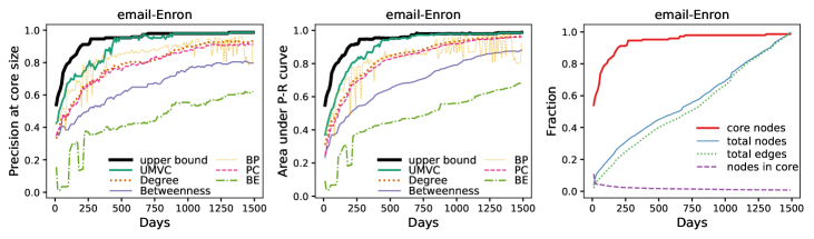
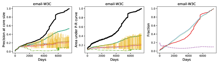
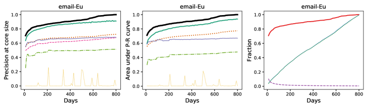
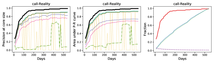
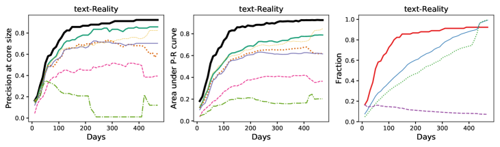
Figure 4. Core recovery performance on five real-world datasets with respect to six methods: our proposed union of minimal vertex covers (UMVC), degree ordering (degree), betweenness centrality (betweenness; [30]), belief propagation (BP; [67]), Borgatti-Everett scores (BE; [8]), and Path-Core scores (PC; [18]). Each dataset has timestamped edges, and we measure the performance of all algorithms every 10 days of real time as the networks evolve. The left column shows precision at the core size, the middle column is the area under the precision recall curve, and the right column tracks the amount of data over time. Our proposed UMVC algorithm performs well on all datasets. BP is sometimes competitive but is susceptible to poor local minima, as evidenced by its erratic performance on several datasets.

Other algorithms for comparison. We compare UMVC against five other methods. First, we consider an ordering of nodes by decreasing degree. This heuristic captures the fact that the nodes outside of $C$ cannot link to each other and that $\lvert C\rvert$ is much smaller than the total number of vertices. This heuristic has previously been used as a baseline for core-periphery identification [58] and is theoretically justified in certain stochastic block models of core-periphery structure [67]. Second, we use betweenness centrality [30] to order the nodes, the idea being that nodes in the core must appear in shortest paths between nodes in the fringe. Third, we use the Path-Core (PC) scores [18] to order the nodes; these scores are a modified version of betweenness centrality, which have been used to identify core-periphery structure in networks [45]. Fourth, we use a scoring measure introduced by Borgatti and Everett (BE) for evaluating core-periphery structure with the core-fringe structure in which we are interested [8]. Formally, the score vector $s$ is the minimizer of the function $\sum_{(i,j)\in E}(A_{ij}-s_{i}s_{j})^{2}$. We use a power-method-like iteration to compute $s$ [15]. Fifth, we use a belief propagation (BP) method designed for stochastic block models of core-periphery structure [67].

Results. We divide the temporal edges of each dataset into 10-day increments and construct an undirected, unweighted, simple graph for the first $10r$ days of activity, $r=1,2,\ldots,\lfloor T/10\rfloor$, where $T$ is the total number of days spanned by the dataset (Table 1). Given the ordering of nodes from each algorithm, we evaluate recovery performance by the precision at core size (P@CS; Fig. 4, left column) and the area under the precision recall curve (AUPRC; Fig. 4, middle column). We emphasize that no algorithm has knowledge of the actual core size. We also provide an upper bound on performance, which for the P@CS metric is the number of non-isolated nodes in the core at the time divided by the total number of core nodes in the dataset and for AUPRC is the performance of an order of nodes that places all of the non-isolated core nodes first and then a random order for the remaining nodes. The right column of Fig. 4 provides statistics on the growth of the network over time.

We observe that, across all datasets, our UMVC algorithm out-performs the degree, betweenness, PC, and BE baselines at essentially nearly all points in time. The belief propagation sometimes exhibits better slightly performance but suffers from erratic performance over time due to landing in local minima; for example, see the recovery performance of the email-W3C dataset in row 2 of Fig. 4. In some cases, belief propagation can hardly pick up any signal, which is the case in the email-Eu dataset (row 3 of Fig. 4). In this dataset, UMVC clearly out-performs other baselines. In the email-Enron dataset, UMVC achieves perfect recovery after around 800 days of activity.

The key reason for the better performance of UMVC is that it uses the fact that the core is a vertex cover. Low-degree nodes that might look like traditional “periphery” nodes in a core-periphery dataset but remain in the core are not picked up by the other algorithms. Core-periphery detection algorithms in network science have traditionally relied on SBM benchmarks, eyeball tests, or heuristic benchmarks [58, 67]. We have already theoretically shown how the SBM induces substantial structure for this problem in our setup, and others have performed similar analysis for block models [67]; thus, this may not be an appropriate benchmark for further analysis. Here, we give some notion of ground truth labels on which to evaluate the algorithms and exploited the vertex cover structure of the problem.

3.2. Timing performance

We also measure the time to run the algorithms on the entire dataset (Table 2). For our UMVC algorithm, we use the union of 300 minimal vertex covers. Tuning the number of vertex covers provides a way for the application user to trade off run-time performance and (potentially) recovery performance. The algorithm was implemented in Julia (Fig. 3). The degree-based ordering was also implemented in Julia, betweenness centrality was computed with the LightGraphs.jl julia package’s implementation of Brandes’ algorithm for sparse graphs [9, 10]. The Path-Cores method was implemented in Python using the NetworkX library, and the Belief Propagation algorithm was implemented in C++. We emphasize that our goal here is to demonstrate the approximate computation times, rather than to compare the most high-performance implementations possible.

The UMVC algorithm takes a few seconds for the email-W3C, email-Enron, reality-call, and reality-text datasets, and about one minute for the email-Eu dataset. This is an order of magnitude faster than belief propagation (BP), and several orders of magnitude faster than betweenness centrality and Path-Core scores (PC). There are approximation algorithms for betweenness centrality, which would be faster than the exact algorithm [6, 32]; however, the weak performance of the exact betweenness-based algorithm on our datasets did not justify our exploration of these approaches.

Table 2. Time to run the algorithms on the largest dataset appearing in Fig. 4. Our proposed union of minimal vertex covers algorithm (UMVC) is fast and provides the best performance on several real-world datasets (see Fig. 4). Here, we use 300 minimal vertex covers in our UMVC algorithm; choosing the number of covers allows the user to tune the running time.

Dataset	UMVC	degree	betweenness [30]	PC [18]	BE [8, 15]	BP [67]
email-W3C	6.5 secs	$<$ 0.01 secs	2.8 mins	1.1 hours	$<$ 0.1 secs	1.0 mins
email-Enron	8.4 secs	$<$ 0.01 secs	2.5 mins	1.8 hours	$<$ 0.1 secs	20.2 mins
email-Eu	1.2 mins	$<$ 0.01 secs	11.8 hours	$>$ 3 days	$<$ 0.9 secs	15.0 mins
call-Reality	2.2 secs	$<$ 0.01 secs	27.9 secs	6.1 mins	$<$ 1.8 secs	4.3 secs
text-Reality	0.5 secs	$<$ 0.01 secs	0.8 secs	11.4 secs	$<$ 0.1 secs	6.8 secs

4. Discussion

Many network datasets are constructed with partial measurements and such data is often “found” in some way that destroys the record of how the measurements were made. Here, we have examined the particular case of graph data where the edges are collected by observing all interactions involving some core set of nodes, but the identity of the core nodes is lost. Such sets of core nodes act as a planted vertex cover in the graph. In addition to developing theory for this problem, we devised a simple and fast algorithm that recovers such cores with extremely high efficacy in several real-world datasets.

There are a number of further directions that would be interesting to consider. First, in order to develop theory and abstract the problem, we assumed that our graphs were simple and undirected. However, there is much richer structure in the data that is generally collected. For example, the interactions in the email, phone call, and text messaging data are directional and could be modeled with a directed graph. Furthermore, we did not exploit the timestamps or the frequency of communication between nodes. One could incorporate this information into a weighted graph model of the data.

Substantial effort has been put forth in the network science community to study mesoscale core-periphery structure in network data. However, the evaluation of such methods has been empirical or evaluated on simple models such as the stochastic block model, which we showed actually induces a substantial amount of structure on the recovery problem. The present work is the first effort to evaluate the recovery of core-periphery-like (i.e., core-fringe) network structure with much more worst-case assumptions through the lens of machine learning with “ground truth” labels on the nodes. We hope that this provides a valuable testbed for evaluating algorithms that reveal core-periphery structure, although we should not take evaluation on ground truth labels as absolute [57].

Software accompanying this paper is available at:

https://github.com/arbenson/FGDnPVC.

Acknowledgments

We thank Jure Leskovec for providing access to the email-Eu data; Mason Porter and Sang Hoon Lee for providing the Path-Core code; and Travis Martin and Thomas Zhang for providing the belief propagation code. This research was supported in part by a Simons Investigator Award and NSF TRIPODS Award #1740822.

References

- [1] E. Abbe. Community detection and stochastic block models: recent developments. arXiv:1703.10146, 2017.
- [2] E. Abbe, A. S. Bandeira, and G. Hall. Exact recovery in the stochastic block model. IEEE Transactions on Information Theory, 62(1):471–487, 2016.
- [3] E. Abbe and C. Sandon. Recovering communities in the general stochastic block model without knowing the parameters. In Advances in Neural Information Processing Systems, pages 676–684, 2015.
- [4] R. Albert and A.-L. Barabási. Statistical mechanics of complex networks. Reviews of Modern Physics, 74(1), 2002.
- [5] N. Alon, M. Krivelevich, and B. Sudakov. Finding a large hidden clique in a random graph. Random Structures and Algorithms, 13(3-4):457–466, 1998.
- [6] D. A. Bader, S. Kintali, K. Madduri, and M. Mihail. Approximating betweenness centrality. In International Workshop on Algorithms and Models for the Web-Graph, pages 124–137. Springer, 2007.
- [7] P. J. Bickel and A. Chen. A nonparametric view of network models and newman–girvan and other modularities. Proceedings of the National Academy of Sciences, 106(50):21068–21073, 2009.
- [8] S. P. Borgatti and M. G. Everett. Models of core/periphery structures. Social Networks, 21(4):375–395, 2000.
- [9] U. Brandes. A faster algorithm for betweenness centrality. The Journal of Mathematical Sociology, 25(2):163–177, 2001.
- [10] U. Brandes. On variants of shortest-path betweenness centrality and their generic computation. Social Networks, 30(2):136–145, 2008.
- [11] R. Breiger. Structures of economic interdependence among nations. Continuities in structural inquiry, pages 353–380, 1981.
- [12] P. Buneman, S. Khanna, and T. Wang-Chiew. Why and where: A characterization of data provenance. In The International Conference on Database Theory, pages 316–330. Springer Berlin Heidelberg, 2001.
- [13] R. S. Burt. Positions in networks. Social Forces, 55(1):93, 1976.
- [14] J. F. Buss and J. Goldsmith. Nondeterminism within . SIAM Journal on Computing, 22(3):560–572, 1993.
- [15] A. L. Comrey. The minimum residual method of factor analysis. Psychological Reports, 11(1):15–18, 1962.
- [16] N. Craswell, A. P. de Vries, and I. Soboroff. Overview of the trec 2005 enterprise track. In TREC, volume 5, pages 199–205, 2005.
- [17] P. Csermely, A. London, L.-Y. Wu, and B. Uzzi. Structure and dynamics of core/periphery networks. Journal of Complex Networks, 1(2):93–123, 2013.
- [18] M. Cucuringu, P. Rombach, S. H. Lee, and M. A. Porter. Detection of core-periphery structure in networks using spectral methods and geodesic paths. European Journal of Applied Mathematics, 27(06):846–887, 2016.
- [19] P. Damaschke. Parameterized enumeration, transversals, and imperfect phylogeny reconstruction. Theoretical Computer Science, 351(3):337–350, 2006.
- [20] P. Damaschke and L. Molokov. The union of minimal hitting sets: Parameterized combinatorial bounds and counting. Journal of Discrete Algorithms, 7(4):391–401, 2009.
- [21] V. Dani and C. Moore. Independent sets in random graphs from the weighted second moment method. In Approximation, Randomization, and Combinatorial Optimization. Algorithms and Techniques, pages 472–482. Springer Berlin Heidelberg, 2011.
- [22] J. Davis and M. Goadrich. The relationship between precision-recall and ROC curves. In Proceedings of the 23rd international conference on Machine Learning. ACM Press, 2006.
- [23] A. Decelle, F. Krzakala, C. Moore, and L. Zdeborová. Asymptotic analysis of the stochastic block model for modular networks and its algorithmic applications. Physical Review E, 84(6), 2011.
- [24] Y. Deshpande and A. Montanari. Finding hidden cliques of size in nearly linear time. Foundations of Computational Mathematics, 15(4):1069–1128, 2014.
- [25] R. G. Downey and M. R. Fellows. Parameterized complexity. Springer Science & Business Media, 2012.
- [26] N. Eagle and A. S. Pentland. Reality mining: sensing complex social systems. Personal and Ubiquitous Computing, 10(4):255–268, 2005.
- [27] D. Easley and J. Kleinberg. Networks, crowds, and markets: Reasoning about a highly connected world. Cambridge University Press, 2010.
- [28] D. Eppstein and D. Strash. Listing all maximal cliques in large sparse real-world graphs. In Experimental Algorithms, pages 364–375. Springer Berlin Heidelberg, 2011.
- [29] U. Feige and D. Ron. Finding hidden cliques in linear time. In 21st International Meeting on Probabilistic, Combinatorial, and Asymptotic Methods in the Analysis of Algorithms, pages 189–204. Discrete Mathematics and Theoretical Computer Science, 2010.
- [30] L. C. Freeman. A set of measures of centrality based on betweenness. Sociometry, 40(1):35, 1977.
- [31] A. Frieze. On the independence number of random graphs. Discrete Mathematics, 81(2):171–175, 1990.
- [32] R. Geisberger, P. Sanders, and D. Schultes. Better approximation of betweenness centrality. In Proceedings of the Meeting on Algorithm Engineering & Expermiments, pages 90–100. Society for Industrial and Applied Mathematics, 2008.
- [33] K. J. Gile and M. S. Handcock. Respondent-driven sampling: An assessment of current methodology. Sociological Methodology, 40(1):285–327, 2010.
- [34] S. P. Hier and J. Greenberg. Surveillance: Power, Problems, and Politics. UBC Press, 2009.
- [35] P. W. Holland, K. B. Laskey, and S. Leinhardt. Stochastic blockmodels: First steps. Social Networks, 5(2):109–137, 1983.
- [36] P. Holme. Core-periphery organization of complex networks. Physical Review E, 72(4), 2005.
- [37] H. V. Jagadish, J. Gehrke, A. Labrinidis, Y. Papakonstantinou, J. M. Patel, R. Ramakrishnan, and C. Shahabi. Big data and its technical challenges. Communications of the ACM, 57(7):86–94, 2014.
- [38] M. Khabbazian, B. Hanlon, Z. Russek, and K. Rohe. Novel sampling design for respondent-driven sampling. Electronic Journal of Statistics, 11(2):4769–4812, 2017.
- [39] M. Kim and J. Leskovec. The network completion problem: Inferring missing nodes and edges in networks. In Proceedings of the 2011 SIAM International Conference on Data Mining, pages 47–58. Society for Industrial and Applied Mathematics, 2011.
- [40] B. Klimt and Y. Yang. Introducing the Enron Corpus. In CEAS, 2004.
- [41] G. Kossinets. Effects of missing data in social networks. Social Networks, 28(3):247–268, 2006.
- [42] D. Koutra, J. T. Vogelstein, and C. Faloutsos. DeltaCon: A principled massive-graph similarity function. In Proceedings of the 2013 SIAM International Conference on Data Mining, pages 162–170. Society for Industrial and Applied Mathematics, may 2013.
- [43] T. Kuny. A digital dark ages? challenges in the preservation of electronic information of electronic information. In 63rd IFLA Council and General Conference, 1997.
- [44] E. O. Laumann, P. V. Marsden, and D. Prensky. The boundary specification problem in network analysis. Research methods in social network analysis, 61:87, 1989.
- [45] S. H. Lee, M. Cucuringu, and M. A. Porter. Density-based and transport-based core-periphery structures in networks. Physical Review E, 89(3), 2014.
- [46] J. Leskovec, J. Kleinberg, and C. Faloutsos. Graphs over time: Densification laws, shrinking diameters and possible explanations. In Proceeding of the eleventh ACM SIGKDD international conference on Knowledge discovery in data mining. ACM Press, 2005.
- [47] J. Leskovec, J. Kleinberg, and C. Faloutsos. Graph evolution: Densification and shrinking diameters. ACM Transactions on Knowledge Discovery from Data, 1(1):2–es, 2007.
- [48] J. Leskovec, K. J. Lang, and M. Mahoney. Empirical comparison of algorithms for network community detection. In Proceedings of the 19th international conference on World Wide Web. ACM Press, 2010.
- [49] C. Lynch. How do your data grow? Nature, 455(7209):28–29, 2008.
- [50] R. Matei, A. Iamnitchi, and P. Foster. Mapping the gnutella network. IEEE Internet Computing, 6(1):50–57, 2002.
- [51] R. Meka, A. Potechin, and A. Wigderson. Sum-of-squares lower bounds for planted clique. In Proceedings of the Forty-Seventh Annual ACM on Symposium on Theory of Computing. ACM Press, 2015.
- [52] T. Monahan, D. J. Phillips, and D. M. Wood. Surveillance and empowerment. Surveillance and Society, 8(2):106–112, 2010.
- [53] E. Mossel, J. Neeman, and A. Sly. Belief propagation, robust reconstruction and optimal recovery of block models. In Conference on Learning Theory, pages 356–370, 2014.
- [54] M. E. J. Newman. The structure and function of complex networks. SIAM Review, 45(2), 2003.
- [55] D. Oard, T. Elsayed, J. Wang, Y. Wu, P. Zhang, E. Abels, J. Lin, and D. Soergel. Trec-2006 at maryland: Blog, enterprise, legal and qa tracks. Technical report, University of Maryland Institute for Advanced Computer Studies, 2006.
- [56] P. Panzarasa, T. Opsahl, and K. M. Carley. Patterns and dynamics of users’ behavior and interaction: Network analysis of an online community. Journal of the American Society for Information Science and Technology, 60(5):911–932, 2009.
- [57] L. Peel, D. B. Larremore, and A. Clauset. The ground truth about metadata and community detection in networks. Science Advances, 3(5):e1602548, 2017.
- [58] P. Rombach, M. A. Porter, J. H. Fowler, and P. J. Mucha. Core-periphery structure in networks (revisited). SIAM Review, 59(3):619–646, 2017.
- [59] D. M. Romero, B. Uzzi, and J. Kleinberg. Social networks under stress. In Proceedings of the 25th International Conference on World Wide Web. ACM Press, 2016.
- [60] C. Seshadhri, A. Pinar, and T. G. Kolda. Fast triangle counting through wedge sampling. In Proceedings of the SIAM Conference on Data Mining, volume 4, page 5, 2013.
- [61] Y. L. Simmhan, B. Plale, and D. Gannon. A survey of data provenance in e-science. ACM SIGMOD Record, 34(3):31, 2005.
- [62] D. A. Spielman. Erdös-Rényi Random Graphs: Warm Up. Graphs and Networks Lecture Notes. http://www.cs.yale.edu/homes/spielman/462/2010/lect3-10.pdf, 2010.
- [63] W.-C. Tan. Research problems in data provenance. IEEE Data Engineering Bulletin, 27:45–52, 2004.
- [64] A. Tsiatas, I. Saniee, O. Narayan, and M. Andrews. Spectral analysis of communication networks using dirichlet eigenvalues. In Proceedings of the 22nd international conference on World Wide Web. ACM Press, 2013.
- [65] Y. Wu, D. W. Oard, and I. Soboroff. An exploratory study of the w3c mailing list test collection for retrieval of emails with pro/con argument. In CEAS, 2006.
- [66] H. Yin, A. R. Benson, J. Leskovec, and D. F. Gleich. Local higher-order graph clustering. In Proceedings of the 23rd ACM SIGKDD International Conference on Knowledge Discovery and Data Mining. ACM Press, 2017.
- [67] X. Zhang, T. Martin, and M. E. J. Newman. Identification of core-periphery structure in networks. Physical Review E, 91(3), 2015.