Semiclassical and quantum behavior of the Mixmaster model in the polymer approach for the isotropic Misner variable

Abstract

We analyze the semi-classical and quantum behavior of the Bianchi IX Universe in the Polymer Quantum Mechanics framework, applied to the isotropic Misner variable, linked to the space volume of the model. The study is performed both in the Hamiltonian and field equations approaches, leading to the remarkable result of a still singular and chaotic cosmology, whose Poincaré return map asymptotically overlaps the standard Belinskii-Khalatnikov-Lifshitz one. In the quantum sector, we reproduce the original analysis due to Misner, within the revised Polymer approach and we arrive to demonstrate that the quantum numbers of the point-Universe still remain constants of motion. This issue confirms the possibility to have quasi-classical states up to the initial singularity. The present study clearly demonstrates that the asymptotic behavior of the Bianchi IX Universe towards the singularity is not significantly affected by the Polymer reformulation of the spatial volume dynamics both on a pure quantum and a semiclassical level.

1 Introduction

The Bianchi IX Universe Landau:1980 ; Misner:1973 is the most interesting among the Bianchi models. In fact, like the Bianchi type VIII, it is the most general allowed by the homogeneity constraint, but unlike the former, it admits an isotropic limit, naturally reached during its evolution Grishchuk:1975 ; Doroshkevich:1973 (see also Kirillov:2002 ; Montani:2008 ), coinciding with the positively curved Robertson-Walker geometry. Furthermore, the evolution of the Bianchi IX model towards the initial singularity is characterized by a chaotic structure, first outlined in Belinskii:1970 in terms of the Einstein equations morphology and then re-analyzed in Hamiltonian formalism by Misner:1969 ; Misner:1969mixmaster . Actually, the Bianchi IX chaotic evolution towards the singularity constitutes, along with the same behavior recovered in Bianchi type VIII, the prototype for a more general feature, characterizing a generic inhomogeneous cosmological model Belinskii:1982 (see also Kirillov:1993 ; Montani:1995 ; Montani:2008 ; Montani:2011 ; Heinzle:2009 ; Barrow:1979 ).

The original interest toward the Bianchi IX chaotic cosmology was due to the perspective, de facto failed, to solve the horizon paradox via such a statistical evolution of the Universe scale factors, from which derives the name, due to C. W. Misner, of the so-called Mixmaster model. However, it was clear since from the very beginning, that the chaotic properties of the Mixmaster model had to be replaced, near enough to the initial singularity (essentially during that evolutionary stage dubbed Planck era of the Universe), by a quantum evolution of the primordial Universe. This issue was first addressed in Misner:1969 , where the main features of the Wheeler-De Witt equation DeWitt:1967 are implemented in the scenario of the Bianchi IX cosmology. This analysis, besides its pioneering character (see also Graham:1994 ; Montani:2008 ), outlined the interesting feature that a quasi-classical state of the Universe, in the sense of large occupation numbers of the wave function, is allowed up to the initial singularity.

More recent approaches to Canonical Quantum Gravity, like the so-called Loop Quantum Gravity Cianfrani:2014 , suggested that the geometrical operators, areas and volumes, are actually characterized by a discrete spectrum Rovelli:1995 . The cosmological implementation of this approach led to the definition of the concept of “Big-Bounce” Ashtekar:2006quantum ; Ashtekar:2006num (i.e. to a geometrical cut-off of the initial singularity, mainly due to the existence of a minimal value for the Universe Volume) and could transform the Mixmaster Model in a cyclic Universe Montani:2018 ; Barrow:2017 . The complete implementation of the Loop Quantum Gravity to the Mixmaster model is not yet available Ashtekar:2009 ; Ashtekar:2011bkl ; Bojowald:2004ra , but general considerations on the volume cut-off led to characterize the semi-classical dynamics as chaos-free Bojowald:2004 . A quantization procedure, able to mimic the cut-off physics contained in the Loop Quantum Cosmology, is the so-called Polymer quantum Mechanics, de facto a quantization on a discrete lattice of the generalized coordinates Ashtekar:2001xp (for cosmological implementations see Corichi:2007pr ; Montani:2013 ; Moriconi:2017 ; Battisti:2008 ; Hossain:2010 ; DeRisi:2007 ; Hassan:2017 ; Seahra:2012 ).

Here, we apply the Polymer Quantum Mechanics to the isotropic variable $\alpha$ of the Mixmaster Universe, described both in the Hamiltonian and field equations representation. We first analyze the Hamiltonian dynamics in terms of the so called semiclassical polymer equations, obtained in the limit of a finite lattice scale, but when the classical limit of the dynamics for $\hbar\rightarrow 0$ is taken. Such a semiclassical approach clearly offers a characterization for the behavior of the mean values of the quantum Universe, in the spirit of the Ehrenfest theorem Sakurai:2011 . This study demonstrates that the singularity is not removed and the chaoticity of the Mixmaster model is essentially preserved, and even enforced in some sense, in this cut-off approach.

Then, in order to better characterize the chaotic features of the obtained dynamics, we translate the Hamiltonian polymer-like dynamics, in terms of the modified Einstein equations, in order to calculate the morphology of the new Poincaré return map, i.e. the modified BKL map.

We stress that, both the reflection rule of the point-Universe against the potential walls and the modified BKL map acquire a readable form up to first order in the small lattice step parameter. Both these two analyses clarify that the chaotic properties of the Bianchi IX model survive in the Polymer formulation and are expected to preserve the same structure of the standard General Relativity case. In particular, when investigating the field equations, we numerically iterate the new map, showing how it asymptotically overlaps to the standard BKL one.

The main merit of the present study is to offer a detailed and accurate characterization of the Mixmaster dynamics when the Universe volume (i.e. the isotropic Misner variable) is treated in a semiclassical Polymer approach, demonstrating how this scenario does not alter, in the chosen representation, the existence of the initial singularity and the chaoticity of the model in the asymptotic neighborhoods of such a singular point.

Finally, we repeat the quantum Misner analysis in the Polymer revised quantization framework and we show, coherently with the semiclassical treatment, that the Misner conclusion about the states with high occupation numbers, still survives: such occupation numbers still behave as constants of motion in the asymptotic dynamics.

It is worth to be noted that imposing a discrete structure to the variable $\alpha$ does not ensure that the Bianchi IX Universe volume has a natural cut-off. In fact, such a volume behaves like $e^{3\alpha}$ and it does not take a minimal (non-zero) value when $\alpha$ is discretized. This fact could suggest that the surviving singularity is a consequence of the absence of a real geometrical cut-off, like in Loop Quantum Cosmology (of which our approach mimics the semi-classical features). However, the situation is subtler, as clarified by the following two considerations.

1. In Montani:2013 , where the polymer approach is applied to the anisotropy variables $\beta_{\pm}$, the Mixmaster chaos is removed like in Bojowald:2004 even if no discretization is imposed on the isotropic (volume) variable. Furthermore, approaching the singularity, the anisotropies classically diverge and their discretization does not imply any intuitive regularization, as de facto it takes place there. The influence of the discretization induced by the Polymer procedure, can affect the dynamics in a subtle manner, non-necessarily predicted by the simple intuition of a cut-off physics, but depending on the details of the induced symplectic structure.

2. In Loop Quantum Gravity, the spectrum of the geometrical spatial volume is discrete, but it must be emphasized that such a spectrum still contains the zero eigenvalue. This observation, when the classical limit is constructed including the suitably weighted zero value, allows to reproduce the continuum properties of the classical quantities. Such a point of view is well-illustrated in Rovelli:2002vp , where the preservation of a classical Lorentz transformation is discussed in the framework of Loop Quantum Gravity. This same consideration must hold in Loop Quantum Cosmology, for instance in Ashtekar:2006quantum , where the position of the bounce is determined by the scalar field parameter, i.e., on a classical level, it depends also on the initial conditions and not only on the quantum modification to geometrical properties of space-time.

Following the theoretical paradigm suggested by the point (ii), the analysis of the Polymer dynamics of the Misner isotropic variable $\alpha$ is extremely interesting because it corresponds to a discretization of the Universe volume, but allowing for the value zero of such a geometrical quantity.

We note that picking, as the phase-space variable to quantize, the scale factor $a=e^{\alpha}$, or any other given power of this, the corresponding Polymer discretization is somehow forced to become singularity-free, i.e. we observe the onset of a Big Bounce. However, in the present approach, based on a logarithmic scale factor, the polymer dynamical scheme offers an intriguing arena to test the Polymer Quantum Mechanics in the Minisuperspace, even in comparison with the predictions of Loop Quantum Cosmology Cianfrani:2014 .

Finally, we are interested in determining the fate of the Mixmaster model chaoticity, which is suitably characterized by the Misner variables representation and whose precise description (i.e. ergodicity of the dynamics, form of the invariant measure) is reached in terms of the Misner-Chitré-like variables Montani:2011 ; Montani:1997 ; Imponente:2001fy , which are double logarithmic scale factors. Although these variables mix the isotropic and anisotropic Misner variables to some extent, the Misner-Chitré time-like variable in the configurational scale, once discretized would not guarantee a minimal value of the universe volume. Thus the motivations for a Polymer treatment of the Mixmaster model in which only the $\alpha$ dynamics is deformed relies on different and converging requests, coming from the cosmological, the statistical and the quantum feature of the Bianchi IX universe.

The paper is organized as follows. In Section 2 we introduce the main kinematic and dynamic features of the Polymer Quantum Mechanics. Then we outline how this singular representation can be connected with the Schrödinger one through an appropriate Continuum Limit.

In Section 3 we describe the dynamics of the homogeneous Mixmaster model as it can be derived through the Einstein field equations. A particular attention is devoted to the Bianchi I and II models, whose analysis is useful for the understanding of the general Bianchi IX (Mixmaster) dynamics.

The Hamiltonian formalism is introduced in Section 4, where we review the semiclassical and quantum properties of the model as it was studied by Misner in Misner:1969 .

Section 5 is devoted to the analysis of the polymer modified Mixmaster model in the Hamiltonian formalism, both from a semiclassical and a quantum point of view. Our results are then compared with the ones derived by some previous models.

In Section 6 the semiclassical behavior of the polymer modified Bianchi I and Bianchi II models is developed through the Einstein equations formalism, while the modified BKL map is derived and its properties discussed from an analytical and numerical point of view in Section 7.

In Section 8 we discuss two important physical issues, concerning the link of the polymer representation with Loop Quantum Cosmology and the implications of a polymer quantization of the whole Minisuperspace variables on the Mixmaster chaotic features.

Finally, in Section 9 brief concluding remarks follow.

2 Polymer Quantum Mechanics

The Polymer Quantum Mechanics (PQM) is a representation of the usual canonical commutation relations (CCR), unitarily nonequivalent to the Schrödinger one. It is a very useful tool to investigate the consequences of the assumption that one or more variables of the phase space are discretized. Physically, it accounts for the introduction of a cutoff. In certain cases where the Schrödinger representation is well-defined, the cutoff can be removed through a certain limiting procedure and the usual Schrödinger representation is recovered, as shown in Corichi:2007pr and summed up in Sec. 2.4.

Many people in the Quantum Gravity community think that there is a maximum theoretical precision achievable when measuring space-time distances, this belief being backed up by valuable although heuristic arguments Salecker-Wigner:1958 ; AmelinoCamelia:1999-Salecker-Wigner ; Hossenfelder:2012jw , so that the cutoff introduced in PQM is assumed to be a fundamental quantity. Some results of Loop Quantum GravityAshtekar:2011 (the discrete spectrum of the area operator) and String TheoryLidsey:1999 (the minimum length of a string) point clearly in the direction of a minimal length scale scenario, too.

PQM was first developed by Ashtekar et al.Ashtekar:2001xp ; Ashtekar:2002 ; Ashtekar:2003 who also credit a previous work of VaradarajanVaradarajan:2000 for some ideas. It was then further refined also by Corichi et al.Corichi:2007pr ; Corichi:2007cqg . They developed the PQM in the expectation to shed some light on the connection between the Planckian-energy Physics of Loop Quantum Gravity and the lower-energy Physics of the Standard Model.

2.1 The Schrödinger representation

Let us consider a quantum one-dimensional free particle with phase space $(q,p)\in\Gamma=\mathbb{R}^{2}$. The standard CCR are summarized by the relation

$$\left[\hat{q},\hat{p}\right]=i\hat{I}$$ (1)

where $\hat{q}$ and $\hat{p}$ are the position and momentum operators respectively and $\hat{I}$ is the identity operator. These operators form a basis for the so called Heisenberg algebraBinz:2008 . At this stage we have not made any assumption regarding the Hilbert space of the theory, yet.

To introduce the Polymer representation in Sec. 2.2, it is convenient to consider also the Weyl algebra $\mathcal{W}$, generated by exponentiation of $\hat{q}$ and $\hat{p}$

$$\hat{U}(\alpha_{i})=e^{i\alpha\hat{q}};\quad\hat{V}(\beta_{i})=e^{i\beta\hat{p}}$$ (2)

where $\alpha$ and $\beta$ are real parameters with the dimension of momentum and length, respectively.

The CCR (1) become

$$\hat{U}(\alpha)\cdot\hat{V}(\beta)=e^{-i\alpha\beta}\hat{V}(\beta)\cdot\hat{U}(\alpha)$$ (3)

where $\cdot$ indicates the product operation of the algebra. All other product combinations commute.

A generic element of the Weyl algebra $W\in\mathcal{W}$ is a finite linear combination

$$W(\alpha,\beta)=\sum_{i}(A_{i}U(\alpha_{i})+B_{i}V(\beta_{i}))$$ (4)

where $A_{i}$ and $B_{i}$ are complex coefficients and the product (3) is extended by linearity. It can be shown that $\mathcal{W}$ has a structure of a $\mathcal{C}^{*}$-algebra.

The Schrödinger representation is obtained as soon as we introduce the Schrödinger Hilbert space of square Lebesgue-integrable functions $\mathcal{H}_{S}=L^{2}(\mathbb{R},dq)$ and the action of the bases operators on it:

$$\hat{q}\psi(q)=q\psi(q);\quad\hat{p}\psi(q)=-i\partial_{q}\psi(q)$$ (5)

where $\psi\in L^{2}(\mathbb{R},dq)$ and $q\in\mathbb{R}$.

2.2 The polymer representation: kinematics

The Polymer representation of Quantum Mechanics can be introduced as follows. First, we consider the abstract states $\ket{\mu}$ of the Polymer Hilbert space $\mathcal{H}_{\text{poly}}$ labeled by the real parameter $\mu$. A generic state of $\mathcal{H}_{\text{poly}}$ consists of a finite linear combination

$$\ket{\Psi}=\sum^{N}_{i=1}a_{i}\ket{\mu_{i}}$$ (6)

where $N\in\mathbb{N}$ and we assume the fundamentals kets to be orthonormal

$$\innerproduct{\mu}{\nu}=\delta_{\mu,\nu}$$ (7)

The Hilbert space $\mathcal{H}_{\text{poly}}$ is the Cauchy completion of the vectors (6) with respect to the product (7). It can be shown that $\mathcal{H}_{\text{poly}}$ is nonseparableCorichi:2007pr .

Two fundamental operators can be defined on this Hilbert space. The “label” operator $\hat{\epsilon}$ and the “displacement” operator $\hat{\boldsymbol{s}}(\lambda)$ with $\lambda\in\mathbb{R}$, which act on the states $\ket{\mu}$ as

$$\hat{\epsilon}\ket{\mu}\coloneqq\mu\ket{\mu};\quad\hat{\boldsymbol{s}}(\lambda)\ket{\mu}\coloneqq\ket{\mu+\lambda}$$ (8)

The $\hat{\boldsymbol{s}}$ operator is discontinuous in $\lambda$ since for each value of $\lambda$ the resulting states $\ket{\mu+\lambda}$ are orthogonal. Thus, there is no Hermitian operator that by exponentiation could generate the displacement operator.

We denote the wave functions in the $p$-polarization as $\psi(p)=\innerproduct{p}{\psi}$, where $\psi_{\mu}(p)=\innerproduct{p}{\mu}=e^{i\mu p}$. The $\hat{V}(\lambda)$ operator defined in (2) shifts the plane waves by $\lambda$

$$\hat{V}(\lambda)\cdot\psi_{\mu}(p)=e^{i\lambda p}e^{i\mu p}=e^{i(\lambda+\mu)p}=\psi_{(\lambda+\mu)}(p)$$ (9)

As expected, $\hat{V}(\lambda)$ can be identified with the displacement operator $\hat{\boldsymbol{s}}(\lambda)$ and the $\hat{p}$ operator cannot be defined rigorously. On the other hand the operator $\hat{q}$ is defined by

$$\hat{q}\cdot\psi_{\mu}(p)=-i\frac{\partial}{\partial p}\psi_{\mu}(p)=\mu e^{i\mu p}=\mu\psi_{\mu}(p)$$ (10)

and thus can be identified with the abstract displacement operator $\hat{\epsilon}$. The reason $\hat{q}$ is said to be discrete is that the eigenvalues of this operator are the labels $\mu$, and even when $\mu$ can take value in a continuum of possible values, they can be regarded as a discrete set, because the states are orthonormal for all values of $\mu$.

The $\hat{V}(\lambda)$ operators form a $\mathcal{C}^{*}$-Algebra and the mathematical theory of $\mathcal{C}^{*}$-AlgebrasArveson:1998 provide us with the tools to characterize the Hilbert space which the wave functions $\psi(p)$ belong to. It is given by the Bohr compactification $\mathbb{R}_{b}$ of the real lineRudin:2011 : $\mathcal{H}_{\text{poly}}=L^{2}(\mathbb{R}_{b},d\mu_{H})$, where the Haar measure $d\mu_{H}$ is the natural choice.

In terms of the fundamental functions $\psi_{\mu}(p)$ the inner product takes the form

$$\begin{split}\innerproduct{\psi_{\mu}}{\psi_{\nu}}\coloneqq&\int_{\mathbb{R}_{b}}d\mu_{H}\bar{\psi_{\mu}}(p)\psi_{\nu}(p)\\ \coloneqq&\lim_{L\to\infty}\frac{1}{2L}\int^{L}_{-L}dp\bar{\psi_{\mu}}(p)\psi_{\nu}(p)=\delta_{\mu,\nu}\end{split}$$ (11)

2.3 Dynamics

Once a definition of the polymer Hilbert space is given, we need to know how to use it in order to analyze the dynamics of a system. The first problem to be faced is that, as it was said after equation (9), the polymer representation isn’t able to describe $\hat{p}$ and $\hat{q}$ at the same time. It is then necessary to choose the “discrete” variable and to approximate its conjugate momentum with a well defined and quantizable function. For the sake of simplicity let us investigate the simple case of a one-dimensional particle described by the Hamiltonian:

$$H=\frac{p^{2}}{2m}+\mathcal{V}(q)$$ (12)

in p-polarization. If we assume that $\hat{q}$ is the discrete operator (in the sense explained in Sec. 2.2), we then need to approximate the kinetic term $\frac{p^{2}}{2m}$ in an appropriate manner. The procedure outlined in Corichi:2007pr consists in the regularization of the theory, through the introduction of a regular graph $\gamma_{\mu_{0}}$ (that is a lattice with spacing $\mu_{0}$), such as:

$$\gamma_{\mu_{0}}=\{q\in\mathbb{R}\ |\ q=n\mu_{0},\ \forall n\in\mathbb{Z}\}$$ (13)

It follows that the only states we shall consider, in order to remain in the graph, are that of the form $\ket{\psi}=\sum_{n}{b_{n}\ket{\mu_{n}}}\in\mathcal{H}_{\gamma_{\mu_{0}}}$, where the $b_{n}$ are coefficients such as $\sum_{n}|b_{n}|^{2}<\infty$ and the $\ket{\mu_{n}}$ (with $\mu_{n}=n\mu_{0}$) are the basic kets of the Hilbert space $\mathcal{H}_{\gamma_{\mu_{0}}}$, which is a separable subspace of $\mathcal{H}_{poly}$. Moreover the action of all operators on these states will be restricted to the graph. Since the exponential operator $\hat{V}(\lambda)=e^{i\lambda p}$ can be identified with the displacement one $\hat{s}$ (Eq. (9)), it is possible to use a regularized version of it ($\hat{V}(\mu_{0})$ such that $\hat{V}(\mu_{0})\ket{\mu_{n}}=\ket{\mu_{n}+\mu_{0}}=\ket{\mu_{n+1}}$) in order to define an approximated version of $\hat{p}$:

$$\hat{p}_{\mu_{0}}\ket{\mu_{n}}=\frac{1}{2i\mu_{0}}[\hat{V}(\mu_{0})-\hat{V}(-\mu_{0})]\ket{\mu_{n}}=\\ =-\frac{i}{2\mu_{0}}(\ket{\mu_{n+1}}-\ket{\mu_{n-1}})$$ (14)

This definition is based on the fact that, for $p<<\frac{1}{\mu_{0}}$, one gets $p\simeq\frac{1}{\mu_{0}}\sin(\mu_{0}p)=\frac{1}{2i\mu_{0}}(e^{i\mu_{0}p}-e^{-i\mu_{0}p})$. From this result it is easy to derive the approximated kinetic term $\hat{p}_{\mu_{0}}^{2}$ by applying the same definition of $\hat{p}_{\mu_{0}}$ two times:

$$\hat{p}_{\mu_{0}}^{2}\ket{\mu_{n}}=\hat{p}_{\mu_{0}}\cdot\hat{p}_{\mu_{0}}\ket{\mu_{n}}=\\ =\frac{1}{4\mu_{0}^{2}}(\ket{\mu_{n+2}}+\ket{\mu_{n-2}}-2\ket{\mu_{n}})$$ (15)

It is now possible to introduce a regularized Hamiltonian operator, which turns out to be well-defined on $\mathcal{H}_{\gamma_{\mu_{0}}}$ and symmetric:

$$\hat{H}_{\mu_{0}}=\frac{\hat{p}_{\mu_{0}}^{2}}{2m}+\mathcal{V}(\hat{q})\in\mathcal{H}_{\gamma_{0}}$$ (16)

In the p-polarization, then, $\hat{p}^{2}_{\mu_{0}}$ acts as a multiplication operator ($\hat{p}^{2}_{\mu_{0}}\psi(p)=\frac{1}{\mu_{0}^{2}}\sin^{2}(\mu_{0}p)\psi(p)$), while $\hat{q}$ acts as a derivative operator ($\hat{q}\psi(p)=i\partial_{p}\psi(p)$).

2.4 Continuum Limit

As we have seen in the previous section, the condition $p<<\frac{1}{\mu_{0}}$ is a fundamental hypothesis of the polymer approach. If this limit is valid for all the orbits of the system to be quantized, such a representation is expected to give results comparable to the ones of the standard quantum representation (based on the Schrödinger equation). This is the reason why a limit procedure from the polymer system to the Schrödinger one is necessary to understand how the two approaches are related. In other words we need to know if, given a polymer wave function defined on the graph $\gamma_{0}$ (with spacing $a_{0}$), it is possible to find a continuous function which is best approximated by the previous one in the limit when the graph becomes finer, that is:

$$\gamma_{0}\to\gamma_{n}=\left\{q_{k}\in\mathbb{R}\ |\ q_{k}=ka_{n},\ \text{with}\ a_{n}=\frac{a_{0}}{2^{n}},\ \forall k\in\mathbb{Z}\right\}$$ (17)

The first step to take in order to answer this question consists in the introduction of the scale $C_{n}$ which is a decomposition of the real line in the union of closed-open intervals with the lattice $\gamma_{n}$ points as extrema, that cover the whole line and do not intersect. For each scale we can then define an effective theory based on the fact that every continuous function can be approximated by another function that is constant on the intervals defined by the lattice. It follows that we can create a link between $\mathcal{H}_{poly}$ and $\mathcal{H}_{S}$ for each scale $C_{n}$:

$$\sum_{m}\psi(ma_{n})\delta_{ma_{n},q}\in\mathcal{H}_{poly}\to\sum_{m}\psi(ma_{n})\chi_{\alpha_{m}}(q)\in\mathcal{H}_{S}$$ (18)

where $\chi_{\alpha_{m}}$ is the characteristic function on the interval $\alpha_{m}=[ma_{n},(m+1)a_{n})$. Thus it is possible to define an effective Hamiltonian $\hat{H}_{C_{n}}$ for each scale $C_{n}$. The set of effective theories is then analyzed by the use of a renormalization procedure Corichi:2007pr , and the result is that the existence of a continuum limit is equivalent to both the convergence of the energy spectrum of the effective theory to the continuous one and the existence of a complete set of renormalized eigenfunctions.

3 The homogeneous Mixmaster model: classical dynamics

With the aim of investigating in Sec. 7 the modifications to the Bianchi IX dynamics produced by the introduction of the Polymer cutoff, in this Section we briefly review some relevant results obtained by Belinskii, Khalatnikov and Lifshitz (BKL) regarding the classical Bianchi IX model. In particular they found that an approximate solution for the Bianchi IX dynamics can be given in the form of a Poincaré recursive map called BKL map. This map is obtained as soon as the exact solutions of Bianchi I and Bianchi II are known. Hence, we will first derive the dynamical solution to the classical Bianchi I and II models.

The Einstein equations of a generic Bianchi model can be expressed in terms of the spatial metric $\eta(t)=\text{diag}[a(t),\\ b(t),c(t)]$ and the constants of structure $\lambda_{l},\lambda_{m},\lambda_{n}$ of the inequivalent isometry group that characterize each Bianchi model, where “$a,b,c$” are said cosmic scale factors and describe the behavior in the synchronous time $t$ of the three independent spatial directionsLandau:1980 .

$$(q_{l})_{\tau\tau}= \frac{1}{2a^{2}b^{2}c^{2}}\left({\lambda_{l}}^{2}a^{4}-{\left(\lambda_{m}b^{2}-\lambda_{n}c^{2}\right)}^{2}\right)$$ (19a)

$$(q_{m})_{\tau\tau}= \frac{1}{2a^{2}b^{2}c^{2}}\left({\lambda_{m}}^{2}b^{4}-{\left(\lambda_{l}a^{2}-\lambda_{n}c^{2}\right)}^{2}\right)$$ (19b)

$$(q_{n})_{\tau\tau}= \frac{1}{2a^{2}b^{2}c^{2}}\left({\lambda_{n}}^{2}c^{4}-{\left(\lambda_{l}a^{2}-\lambda_{m}b^{2}\right)}^{2}\right)$$ (19c)

$${(q_{l}+q_{m}+q_{n})}_{\tau\tau}={(q_{l})}_{\tau}{(q_{m})}_{\tau}+{(q_{l})}_{\tau}{(q_{n})}_{\tau}+{(q_{m})}_{\tau}{(q_{n})}_{\tau}$$ (20)

where the logarithmic variable $q_{l}(\tau),q_{m}(\tau),q_{n}(\tau)$ and logarithmic time $\tau$ are defined as such:

$$q_{l}=2\ln a,\quad q_{m}=2\ln b,\quad q_{n}=2\ln c,\quad dt=(abc)d\tau$$ (21)

and the subscript $\Box_{\tau}$ is a shorthand for the derivative in $\tau$. The isometry group characteristic of Bianchi IX is the SO(3) group. The Class A Bianchi modelsMontani:2011 (of which Bianchi I,II and IX are members) are set apart just by those three constants of structure.

3.1 Bianchi I

The Bianchi I model in void is also called Kasner solutionWainwright:2008 . By substituting in Eqs (19) the Bianchi I constants of structure $\lambda_{l}=0,\lambda_{m}=0,\lambda_{n}=0$, we get the simple equations of motion:

$${(q_{l})}_{\tau\tau}={(q_{m})}_{\tau\tau}={(q_{n})}_{\tau\tau}=0$$ (22)

whose solution can be given as a function of the logarithmic time $\tau$ and four parameters:

$$\begin{dcases}q_{l}(\tau)=2\Lambda p_{l}\tau\\ q_{m}(\tau)=2\Lambda p_{m}\tau\\ q_{n}(\tau)=2\Lambda p_{n}\tau\end{dcases}$$ (23)

where $p_{l},p_{m},p_{n}$ are said Kasner indices and $\Lambda$ is a positive constant that will have much relevance in Section 6.1. It is needed to ensure that the sum of Kasner indices is always one:

$$p_{l}+p_{m}+p_{n}=1$$ (24)

From (23) and (21), if we exploit the constraint (24), we obtain

$$\tau=\frac{1}{\Lambda}\ln(\Lambda t)$$ (25)

From relation (25) stems the appellative “logarithmic time” for the time variable $\tau$.

By substituting the Bianchi I equations of motion (22) and their solution (23) into (20), after applying the constraint (24), we find the additional constraint

$${p_{l}}^{2}+{p_{m}}^{2}+{p_{n}}^{2}=1$$ (26)

With the exception of the null measure set $(p_{l},p_{m},p_{n})=(0,0,1)$ and $(p_{l},p_{m},p_{n})=(-1/3,2/3,2/3)$, Kasner indices are always different from each other and one of them is always negative. The $(0,0,1)$ case can be shown to be equivalent to the Minkowski space-time. It is customary to order the Kasner indices from the smallest to the greatest $p_{1}<p_{2}<p_{3}$. Since the three variables $p_{1},p_{2},p_{3}$ are constrained by equations (24) and (26), they can be expressed as functions of a unique parameter $u$ as

$$p_{1}(u)=\tfrac{-u}{1+u+u^{2}},~{}~{}p_{2}(u)=\tfrac{1+u}{1+u+u^{2}},~{}~{}p_{3}(u)=\tfrac{u(1+u)}{1+u+u^{2}}$$ (27)

$$1\leq u<+\infty$$ (28)

The range and the values of the Kasner indices are portrayed in Fig. 1.

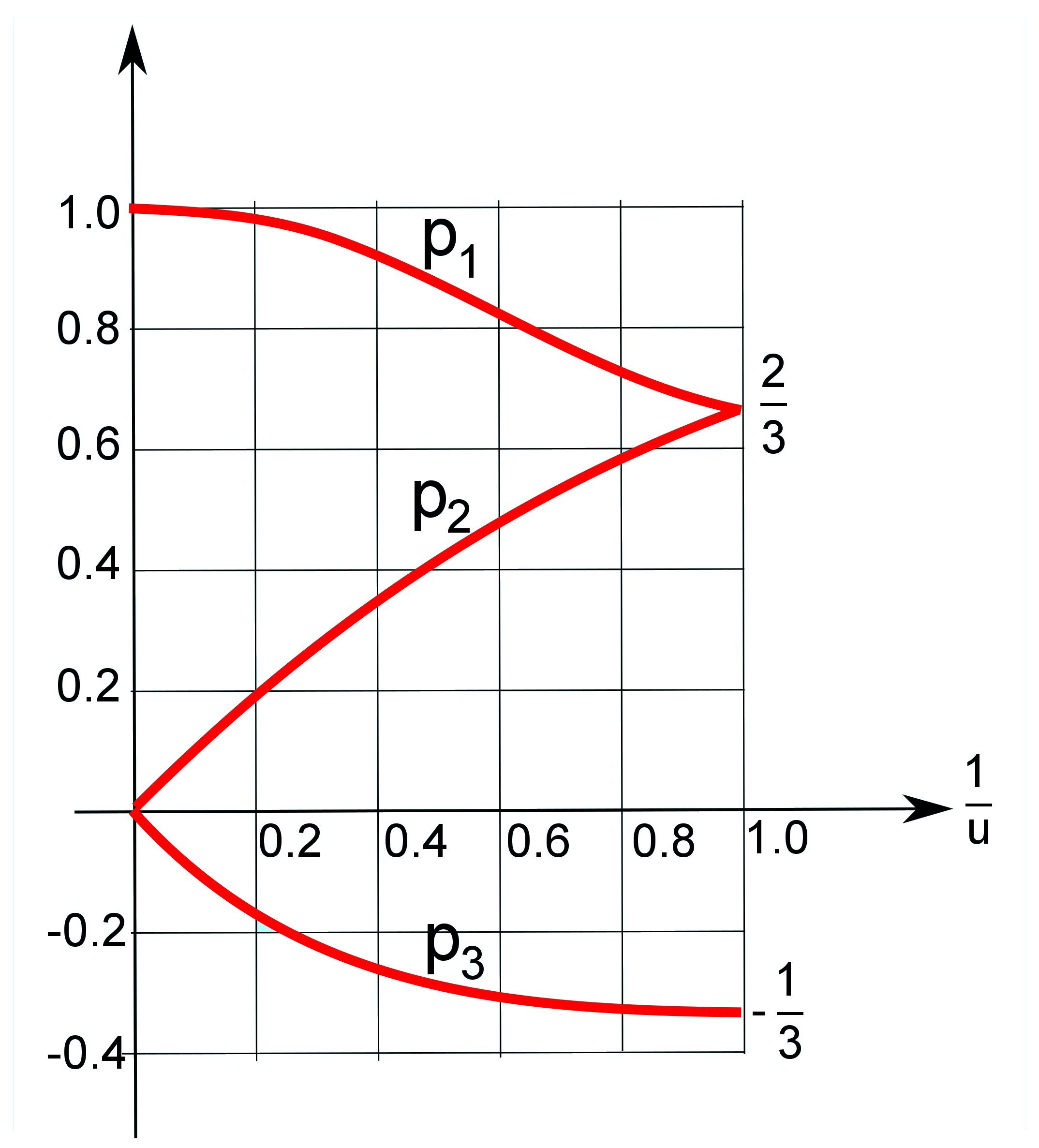
Figure 1: Kasner indices as functions of the inverse of the $u$ parameter. This figure was taken from wiki:BKL and is released under CC BY-SA 3.0 license.

Excluding the Minkowskian case $(0,0,1)$, for any choice of the Kasner indices, the spatial metric $\eta=\text{diag}(t^{2p_{l}},t^{2p_{m}},t^{2p_{n}})$ has a physical naked singularity, called also Big Bang, when $t=0$ (or $\tau\to-\infty$).

3.2 Bianchi II

A period in the evolution of the Universe when the r.h.s of (19) can be neglected, and the dynamics is Bianchi I-like, is called Kasner regime or Kasner epoch. In this Section we show how Bianchi II links together two different Kasner epochs at $\tau\to-\infty$ and $\tau\to\infty$. A series of successive Kasner epochs, where one cosmic scale factor increases monotonically, is called a Kasner era.

Again, after substituting the Bianchi II structure constants $\lambda_{l}=1,\lambda_{m}=0,\lambda_{n}=0$ into Eqs (19), we get

$${(q_{l})}_{\tau\tau}=-e^{2q_{l}}$$ (29a)

$${(q_{m})}_{\tau\tau}={(q_{n})}_{\tau\tau}=e^{2q_{l}}$$ (29b)

It should be noted that the conditions

$${(q_{l})}_{\tau\tau}+{(q_{m})}_{\tau\tau}={(q_{l})}_{\tau\tau}+{(q_{n})}_{\tau\tau}=0$$ (30)

hold for every $\tau$.

Let us consider the explicit solutions of equations (29)

$${(q_{l})}(\tau)= \ln(c_{1}\sech(\tau c_{1}+c_{2}))$$ (31a)

$${(q_{m})}(\tau)= 2c_{3}+2\tau c_{4}-\ln(c_{1}\sech(\tau c_{1}+c_{2}))$$ (31b)

$${(q_{n})}(\tau)= 2c_{5}+2\tau c_{6}-\ln(c_{1}\sech(\tau c_{1}+c_{2}))$$ (31c)

where $c_{1},\dots,c_{6}$ are integration constants. We now analyze how (31) behave as the time variable $\tau$ approaches $+\infty$ and $-\infty$ (remembering also equation (25)). By taking the asymptotic limit to $\pm\infty$, we note that a Kasner regime at $+\infty$ is “mapped” to another Kasner regime at $-\infty$, but with different Kasner indices.

$$\begin{dcases}p_{l}=\tfrac{{(q_{l})}_{\tau}}{2\Lambda}=\tfrac{-c_{1}/2}{c_{4}+c_{6}+c_{1}/2}\\ p_{m}=\tfrac{{(q_{m})}_{\tau}}{2\Lambda}=\tfrac{c_{4}+c_{1}/2}{c_{4}+c_{6}+c_{1}/2}\\ p_{n}=\tfrac{{(q_{n})}_{\tau}}{2\Lambda}=\tfrac{c_{6}+c_{1}/2}{c_{4}+c_{6}+c_{1}/2}\end{dcases}~{}\begin{dcases}p^{\prime}_{l}=\tfrac{{(q_{l})}_{\tau}}{2\Lambda}=\tfrac{c_{1}/2}{c_{4}+c_{6}-c_{1}/2}\\ p^{\prime}_{m}=\tfrac{{(q_{m})}_{\tau}}{2\Lambda}=\tfrac{c_{4}-c_{1}/2}{c_{4}+c_{6}-c_{1}/2}\\ p^{\prime}_{n}=\tfrac{{(q_{n})}_{\tau}}{2\Lambda}=\tfrac{c_{6}-c_{1}/2}{c_{4}+c_{6}-c_{1}/2}\end{dcases}$$ (32)

where we have exploited the notation of equation (23). Both these sets of indices satisfy the two Kasner relations (24) and (26).

The old (the unprimed ones) and the new indices (the primed ones) are related by the BKL map, that can be given in the form of the new primed Kasner indices $p_{l}^{\prime},p_{m}^{\prime},p_{n}^{\prime}$ and $\Lambda^{\prime}$ as functions of the old ones. To calculate it we need at least four relations between the new and old Kasner indices $f_{i}(p_{l},p_{m},p_{n},\Lambda,p^{\prime}_{l},p^{\prime}_{m},p^{\prime}_{n},\Lambda^{\prime})=0$ with $i=1,\dots,4$. Then we can invert these relations to find the BKL map.

One $f_{i}$ is simply the sum of the primed Kasner indices (that is the primed version of (24)). Other two relations can be obtained from (30):

$$\Lambda(p_{l}+p_{m})= \Lambda^{\prime}(p^{\prime}_{l}+p^{\prime}_{m})$$ (33)

$$\Lambda(p_{l}+p_{n})= \Lambda^{\prime}(p^{\prime}_{l}+p^{\prime}_{n})$$ (34)

The fourth relation is obtained by direct comparison of the asymptotic limits (32), and for this reason we will call it asymptotic relation.

$$\Lambda p_{l}=-(\Lambda^{\prime}p^{\prime}_{l})$$ (35)

All other relations that can be obtained from (32) are equivalent to (35).

Finally, by inverting the four relations (24),(33), (34),
(35) and assuming again that $p_{l}$ is the negative Kasner index $p_{1}$, we finally get the classical BKL map:

$$p^{\prime}_{l}=\frac{|p_{l}|}{1-2|p_{l}|},\quad p^{\prime}_{m}=\frac{p_{m}-2|p_{l}|}{1-2|p_{l}|},\quad p^{\prime}_{n}=\frac{p_{n}-2|p_{l}|}{1-2|p_{l}|},$$ (36)

$$\Lambda^{\prime}=(1-2|p_{l}|)\Lambda$$

The main feature of the BKL map is the exchange of the negative index between two different directions. Therefore, in the new epoch, the negative power is no longer related to the $l$-direction and the perturbation to the new Kasner regime (which is linked to the $l$-terms on the r.h.s. of Eq. (19)) is damped and vanishes towards the singularity: the new (primed) Kasner regime is stable towards the singularity.

If we then insert the parametrization (27) and (28) into the BKL map (36) just found, we get that the map in the $u$ parameter is simple-looking.

$$\begin{dcases}p_{l}=p_{1}(u)\\ p_{m}=p_{2}(u)\\ p_{n}=p_{3}(u)\end{dcases}\xrightarrow{\text{BKL map}}\begin{dcases}p^{\prime}_{l}=p_{2}(u-1)\\ p^{\prime}_{m}=p_{1}(u-1)\\ p^{\prime}_{n}=p_{3}(u-1)\end{dcases}$$ (37)

We emphasize that the role of the negative index is swapped between the $l$ and the $m$-direction.

3.3 Bianchi IX

Here we briefly explain how the BKL map can be used to characterize the Bianchi IX dynamics. This is possible because it can be shown Montani:2011 that the Bianchi IX dynamical evolution is made up piece-wise by Bianchi I and II-like “blocks”.

First, we take a look again at the Einstein equations (19): but now we substitute the Bianchi IX structure constants $\lambda_{l}=1,\lambda_{m}=1,\lambda_{n}=1$ into them to get the Einstein equations for Bianchi IX:

$${(q_{l})}_{\tau\tau}={(b^{2}-c^{2})}^{2}-a^{4}$$ (38)

$${(q_{m})}_{\tau\tau}={(a^{2}-c^{2})}^{2}-b^{4}$$

$${(q_{n})}_{\tau\tau}={(a^{2}-b^{2})}^{2}-c^{4}$$

Eq. (20) stays valid for every Bianchi model.

Again, we assume an initial Kasner regime, where the negative Kasner index $p_{1}$ is associated with the $l$-direction. Thus, the “exploding” cosmic scale factor in the r.h.s. of (38) is identified again with $a$. By retaining in the r.h.s. of (38) only the terms that grow towards the singularity, we obtain a system of ordinary differential equations in time completely similar to the one just encountered for Bianchi II (29), with the only caveat that now there is no initial condition (i.e. no choice of the initial Kasner indices) such that the initial or final Kasner regimes are stable towards the singularity.

This because all the cosmic scale factors $\{a,b,c\}$ are treated on an equal footing in the r.h.s. of (38). After every Kasner epoch or era, no matter on which axis the negative index is swapped, there will always be a perturbation in the Einstein equations (38) that will make the Kasner regime unstable. We thus have an infinite series of Kasner eras alternating and accumulating towards the singularity.

Given an initial $u$ parameter, the BKL map that takes it to the next one $u^{\prime}$ is

$$u^{\prime}=\begin{dcases}u-1~{}~{}\text{for}~{}~{}u>2\\ \frac{1}{u-1}~{}~{}\text{for}~{}~{}u\leq 2\\ \end{dcases}$$ (39)

Let us assume an initial $u_{0}=k_{0}+x_{0}$, where $k_{0}=[u_{0}]$ is the integer part and $x_{0}=u_{0}-[u_{0}]$ is the fractional part. If $x_{0}$ is irrational, as it is statistically and more general to infer, after the $k_{0}$ Kasner epochs that make up that Kasner era, its inverse $1/x_{0}$ would be irrational, too. This inversion happens infinitely many times until the singularity is reached and is the source of the chaotic features of the BKL mapBarrow:1981 ; Barrow:1982 ; Khalatnikov:1984hzi ; Lifshitz:1971 ; Montani:1997 ; Szydlowski:1993 .

4 Hamiltonian Formulation of the Mixmaster model

In this section we summarize some important results obtained applying the R. Arnowitt, S. Deser and C.W. Misner (ADM) Hamiltonian methods to the Bianchi models. The main benefit of this approach is that the resulting Hamiltonian system resembles the simple one of a pinpoint particle moving in a potential well. Moreover it provides a method to quantize the system through the canonical formalism.

The line element for the Bianchi IX model is:

$$ds^{2}=N^{2}(t)dt^{2}+\frac{1}{4}e^{2\alpha}{(e^{2\beta})}_{ij}\sigma_{i}\sigma_{j}$$ (40)

where $N$ is the Lapse Function, characteristic of the canonical formalism and $\sigma_{i}$ are 1-forms depending on the Euler angles of the SO(3) group of symmetry. $\beta_{ij}$ is a diagonal, traceless matrix and so it can be parameterized in terms of the two independent variables $\beta_{\pm}$ as $\beta_{ij}=(\beta_{+}+\sqrt{3}\beta_{-},\beta_{+}-\sqrt{3}\beta_{-},-2\beta_{+})$. The factor $\frac{1}{4}$ is chosen (following Misner:1969 ) so that when $\beta_{ij}=0$, we obtain just the standard metric for a three-sphere of radius $r=e^{\alpha}$. Thus for $\beta=0$ this metric is the Robertson-Walker positive curvature metric. The variables $(\alpha,\beta_{\pm})$ were introduced by C.W. Misner in Misner:1969mixmaster ; $\alpha$ describes the expansion of the Universe, i.e. its volume changes $(\mathcal{V}\propto e^{3\alpha})$, while $\beta_{\pm}$ are related to its anisotropies (shape deformations). The kinetic term of the Hamiltonian of the Bianchi models, written in the Misner variables, results to be diagonal; we can then write, following Arnowitt:1960pr , the super-Hamiltonian for the Bianchi models simply as:

$$\mathcal{H}_{B}=\frac{N\kappa}{3(8\pi)^{2}}e^{-3\alpha}\left(-p_{\alpha}^{2}+p_{+}^{2}+p_{-}^{2}+\frac{3(4\pi)^{4}}{\kappa^{2}}e^{4\alpha}V_{B}(\beta_{\pm})\right)$$ (41)

where $(p_{\alpha},p_{\pm})$ are the conjugate momenta to $(\alpha,\beta_{\pm})$ respectively and N is the lapse function. It should be noted that the corresponding super-Hamiltonian constraint $\mathcal{H}_{B}=0$ describes the evolution of a point $\beta=(\beta_{+},\beta_{-})$, that we call $\beta$-point, in function of a new time coordinate $\alpha$ (that is the shape of the Universe in function of its volume). Such point is subject to the anisotropy potential $V_{B}(\beta_{\pm})$ which is a non-negative function of the anisotropy coordinates, whose explicit form depends on the Bianchi model considered. In particular Bianchi type I corresponds to the $V_{B}=0$ case (free particle), Bianchi type II potential corresponds to a single, infinite exponential wall $\left(V_{B}=e^{-8\beta_{+}}\right)$, while for Bianchi type IX we have a closed domain expressed by:

$$V_{B}(\beta_{\pm})=2e^{4\beta_{+}}\left(\cosh(4\sqrt{3}\beta_{-})-1\right)+\\ -4e^{2\beta_{+}}\cosh(2\sqrt{3}\beta_{-})+e^{-8\beta_{+}}$$ (42)

The potential  (42) has steep exponential walls with the symmetry of an equilateral triangle with flared open corners, as we can see from Fig. 2. The presence of the term $e^{4\alpha}$ in (41), moreover, causes the potential walls to move outward as we approach the cosmological singularity $(\alpha\to-\infty)$.

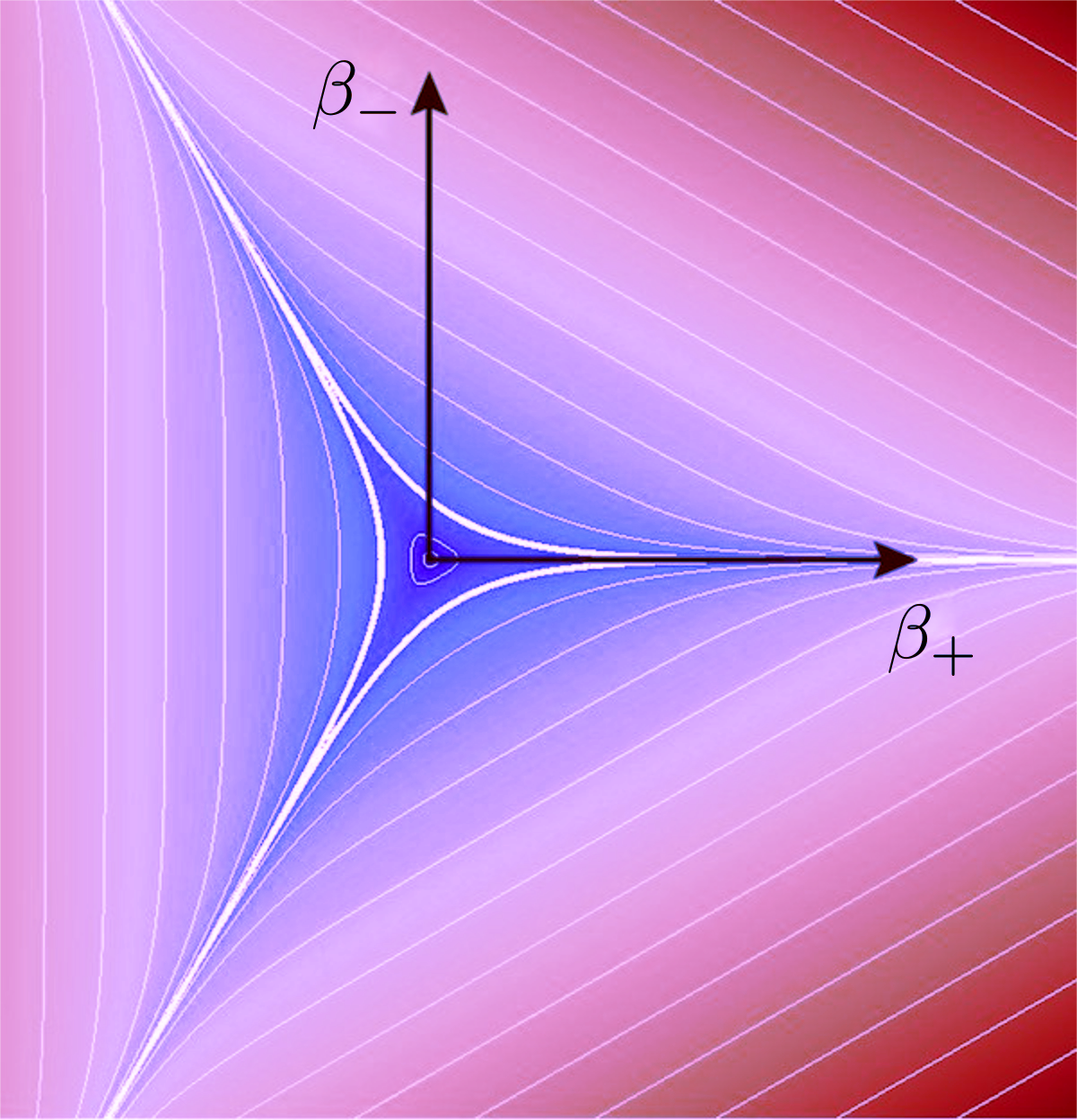
Figure 2: Equipotentials of the function $V_{B}(\beta_{\pm})$ in the $(\beta_{+},\beta_{-})$-plane. Here we can see that far from the origin the function has the symmetry of an equilateral triangle, while near the origin $(V_{B}<1)$ the equipotentials are closed curves.

Following the ADM reduction procedure, we can solve the super-Hamiltonian constraint (41) with respect to the momentum conjugate to the new time coordinate of the phase-space (i.e. $\alpha$). The result is the so-called reduced Hamiltonian $H_{ADM}$:

$$H_{ADM}\coloneqq-p_{\alpha}=\sqrt{p_{+}^{2}+p_{-}^{2}+\frac{3(4\pi)^{4}}{\kappa}e^{4\alpha}V_{B}(\beta_{\pm})}$$ (43)

from which we can derive the classical dynamics of the model by solving the corresponding Hamilton’s equations:

$$\beta^{\prime}_{\pm} \equiv\frac{d\beta_{\pm}}{d\alpha}=\frac{\partial H_{ADM}}{\partial p_{\pm}}$$ (44a)

$$p^{\prime}_{\pm} \equiv\frac{dp_{\pm}}{d\alpha}=-\frac{\partial H_{ADM}}{\partial\beta_{\pm}}$$ (44b)

$$H^{\prime}_{ADM} \equiv\frac{dH_{ADM}}{d\alpha}=\frac{\partial H_{ADM}}{\partial\alpha}$$ (44c)

It should be noted that the choice $\dot{\alpha}=1$ fixes the temporal gauge $N_{ADM}=\frac{6(4\pi)^{2}}{H_{ADM}\kappa}e^{3\alpha}$.

Since we are interested in the dynamics of the model near the singularity $(\alpha\to-\infty)$ and because of the steepness of the potential walls, we can consider the $\beta$-point to spend most of its time moving as a free particle (far from the potential wall $V_{B}\simeq 0$), while $V_{B}(\beta_{\pm})$ is non-negligible only during the short time of a bounce against one of the three walls. It follows that we can separate the analysis into two different phases. As far as the free motion phase (Bianchi type I approximation) is concerned, we can derive the velocity of the $\beta$-point from the first of Eqs. (44) (with $V_{B}=0$), obtaining:

$$\beta^{\prime}\equiv\sqrt{\beta^{\prime 2}_{+}+\beta^{\prime 2}_{-}}=1$$ (45)

It remains to study the bounce against the potential. Following Misner:1969 we can summarize the results of this analysis in three points: (i) The position of the potential wall is defined as the position of the equipotential in the $\beta$-plane bounding the region in which the potential terms are significant. The wall turns out to have velocity $|\beta^{\prime}_{wall}|\equiv\frac{d\beta_{wall}}{d\alpha}=\frac{1}{2}$, that is one half of the $\beta$-point velocity. So a bounce is indeed possible. (ii) Every bounce occurs according to the reflection law:

$$\sin\theta_{i}-\sin\theta_{f}=\frac{1}{2}\sin(\theta_{i}+\theta_{f})$$ (46)

where $\theta_{i}$ and $\theta_{f}$ are the incidence and the reflection angles respectively. (iii) The maximum incidence angle for the $\beta$-point to have a bounce against a specific potential wall turns out to be:

$$\theta_{max}=\arccos\left(\frac{1}{2}\right)=\frac{\pi}{3}$$ (47)

Because of the triangular symmetry of the potential, this result confirms the fact that a bounce against one of the three walls always happens. It follows that the $\beta$-point undergoes an infinite series of bounces while approaching the singularity and, sooner or later, it will assume all the possible directions, regardless the initial conditions. In short we are dealing with a pinpoint particle which undergoes an uniform rectilinear motion marked by the constants of motion $(p_{+},p_{-})$ until it reach a potential wall. The bounce against this wall has the effect of changing the values of $p_{\pm}$. After that, a new phase of uniform rectilinear motion (with different constants of motion) starts. If we remember that the free particle case corresponds to the Bianchi type I model, whose solution is the Kasner solution (see Sec. 3.1), we recover the sequence of Kasner epochs that characterizes the BKL map (Sec. 3.3).

In conclusion, it is worth mentioning that, through the analysis of the geometrical properties of the scheme outlined so far near the cosmological singularity, we can obtain a sort of conservation law, that is:

$$\langle{H_{ADM}\alpha}\rangle=\text{const}$$ (48)

Here the symbol $\langle{...}\rangle$ denotes the average value of $H_{ADM}\alpha$ over a large number of runs and bounces. In fact, although it is not a constant, this quantity acquires the same constant value just before each bounce: $H^{n}_{ADM}\alpha_{n}=H^{n+1}_{ADM}\alpha_{n+1}$. In this sense quantities with this property will be named adiabatic invariants.

4.1 Quantization of the Mixmaster model

Near the Cosmological Singularity some quantum effects are expected to influence the classical dynamics of the model. The use of the Hamiltonian formalism enables us to quantize the cosmological theory in the canonical way with the aim of identify such effects.

Following the canonical formalism Misner:1969 , we can introduce the basic commutation relations $[\hat{\beta}_{a},\hat{p}_{b}]=i\delta_{ab}$, which can be satisfied by choosing $\hat{p}_{a}=-i\frac{\partial}{\partial\beta_{a}}$. Hence all the variables become operators and the super-Hamiltonian constraint (41) is written in its quantum version ($\hat{\mathcal{H}}\Psi(\alpha,\beta_{\pm})=0$) i.e. the Wheeler-De Witt (WDW) equation:

$$\left[\frac{\partial^{2}}{\partial\alpha^{2}}-\frac{\partial^{2}}{\partial\beta_{+}^{2}}-\frac{\partial^{2}}{\partial\beta_{-}^{2}}+\frac{3(4\pi)^{4}}{\kappa^{2}}e^{4\alpha}V_{B}(\beta_{\pm})\right]\Psi(\alpha,\beta_{\pm})=0$$ (49)

The function $\Psi(\alpha,\beta_{\pm})$ is the wave function of the Universe, which we can choose of the form:

$$\Psi(\alpha,\beta_{\pm})=\sum_{n}\chi_{n}(\alpha)\phi_{n}(\alpha,\beta_{\pm})$$ (50)

If we assume the validity of the adiabatic approximation (see Montani:2013 )

$$|\partial_{\alpha}\chi_{n}(\alpha)|>>|\partial_{\alpha}\phi_{n}(\alpha,\beta_{\pm})|$$ (51)

we can solve the WDW equation by separation of variables. In particular the eigenvalues $E_{n}$ of the reduced Hamiltonian (43) are obtained from those of the equation $\hat{H}_{ADM}\phi_{n}=E_{n}^{2}\phi_{n}$ that is:

$$\left[-\frac{\partial^{2}}{\partial\beta_{+}^{2}}-\frac{\partial^{2}}{\partial\beta_{-}^{2}}+\frac{3(4\pi)^{4}}{\kappa^{2}}e^{4\alpha}V_{B}(\beta_{\pm})\right]\phi_{n}(\alpha,\beta_{\pm})=E_{n}^{2}\phi_{n}$$ (52)

The result, achieved by approximating the triangular potential with a quadratic box with infinite vertical walls and the same area of the triangular one $(A=\frac{3}{4}\sqrt{3}\alpha^{2})$, turns out to be:

$$E_{n}\sim\frac{2\pi}{3^{3/4}}\sqrt{n^{2}+m^{2}}\ \alpha^{-1}=\frac{a_{n}}{\alpha}$$ (53)

where $n,m$ are the integer and positive quantum numbers related to the anisotropies $\beta_{\pm}$.

An important conclusion that C.W. Misner derived from this analysis is that quasi-classical states (i.e. quantum states with very high occupation numbers) are preserved during the evolution of the Universe towards the singularity. In fact if we substitute the quasi-classical approximation $H\simeq E_{n}$ in (48) and we study it in the limit $\alpha\to-\infty$, we find:

$$\langle n^{2}+m^{2}\rangle=\text{const}$$ (54)

We can therefore conclude that if we assume that the present Universe is in a quasi-classical state of anisotropy ($n^{2}+m^{2}>>1$), then, as we extrapolate back towards the Cosmological Singularity, the quantum state of the Universe remains always quasi-classical.

5 Mixmaster model in the Polymer approach

Here the Hamiltonian formalism introduced in Sec. 4 is used for the analysis of the dynamics of the modified Mixmaster model. We choose to apply the polymer representation to the isotropic variable $\alpha$ of the system due to its deep connection with the volume of the Universe. As a consequence we will need to find an approximated operator for the conjugate momentum $p_{\alpha}$, while the anisotropy variables $\beta_{\pm}$ will remain unchanged from the standard case.

The introduction of the polymer representation consists in the formal substitution, derived in Sec. 2.3:

$$p_{\alpha}^{2}\to\frac{1}{\mu^{2}}\sin^{2}(\mu p_{\alpha})$$ (55)

which we apply to the super-Hamiltonian constraint $\mathcal{H}_{B}=0$ (with $\mathcal{H}_{B}$ defined in (41)):

$$\frac{N\kappa}{3(8\pi)^{2}}e^{-3\alpha}\left(-\frac{1}{\mu^{2}}\sin^{2}(\mu p_{\alpha})+p_{+}^{2}+p_{-}^{2}+\right.\\ +\left.\frac{3(4\pi)^{4}}{\kappa^{2}}e^{4\alpha}V_{B}(\beta_{\pm})\right)=0$$ (56)

In what follows we will use the ADM reduction formalism in order to study the new model both from a semiclassical and a quantum point of view.

5.1 Semiclassical Analysis

First of all we derive the reduced polymer Hamiltonian
$(H_{\alpha}\coloneqq-p_{\alpha})$ from (56):

$$H_{\alpha}=\frac{1}{\mu}\arcsin\left(\sqrt{\mu^{2}\left[p_{+}^{2}+p_{-}^{2}+\frac{3(4\pi)^{4}}{\kappa^{2}}e^{4\alpha}V_{B}(\beta_{\pm})\right]}\right)$$ (57)

where the condition $0\leq\mu^{2}(p_{+}^{2}+p_{-}^{2}+\frac{3(4\pi)^{4}}{\kappa^{2}}e^{4\alpha}V_{B}(\beta_{\pm}))\leq 1$ has to be imposed due to the presence of the function arcsine. The dynamics of the system is then described by the deformed Hamilton’s equations (that come from Eqs. (44) with $H_{ADM}\equiv H_{\alpha}$):

$$\beta^{\prime}_{\pm} =\frac{p_{\pm}}{\sqrt{(p^{2}+\frac{3(4\pi)^{4}}{\kappa^{2}}e^{4\alpha}V_{B})[1-\mu^{2}(p^{2}+\frac{3(4\pi)^{4}}{\kappa^{2}}e^{4\alpha}V_{B})]}}$$ (58a)

$$p^{\prime}_{\pm} =-\frac{\frac{3(4\pi)^{4}}{2\kappa^{2}}e^{4\alpha}\frac{\partial V_{B}}{\partial\beta_{\pm}}}{\sqrt{(p^{2}+\frac{3(4\pi)^{4}}{\kappa^{2}}e^{4\alpha}V_{B})[1-\mu^{2}(p^{2}+\frac{3(4\pi)^{4}}{\kappa^{2}}e^{4\alpha}V_{B})]}}$$ (58b)

$$H^{\prime}_{\alpha} =\frac{\frac{6(4\pi)^{4}}{\kappa^{2}}e^{4\alpha}V_{B}}{\sqrt{[1-\mu^{2}(p^{2}+\frac{3(4\pi)^{4}}{\kappa^{2}}e^{4\alpha}V_{B})](p^{2}+\frac{3(4\pi)^{4}}{\kappa^{2}}e^{4\alpha}V_{B})}}$$ (58c)

where the prime stands for the derivative with respect to $\alpha$ and $p^{2}=p_{+}^{2}+p_{-}^{2}$.

As for the standard case, we start by studying the simplest case of $V_{B}=0$ (Bianchi I approximation), which corresponds to the phase when the $\beta$-point is far enough from the potential walls. Here the persistence of a cosmological singularity can be easily demonstrated since $\alpha$ results to be linked to the time variable $t$ through a logarithmic relation (as we will see later in Eq. (90a)): $\alpha\sim\ln(t)\underset{t\to 0}{\longrightarrow}-\infty$. Moreover the anisotropy velocity of the particle can be derived from Eq. (58a) (while $p_{\pm}$ and $H_{\alpha}$ are constants of motion) and the result is:

$$\beta^{\prime}\equiv\sqrt{\beta^{\prime 2}_{+}+\beta^{\prime 2}_{-}}=\frac{1}{\sqrt{1-\mu^{2}p^{2}}}\coloneqq r_{\alpha}(\mu,p_{\pm})$$ (59)

Thus the modified anisotropy velocity depends on the constants of motion of the system, and it turns out to be always greater than the standard one $(r_{\alpha}(\mu,p_{\pm})>1,\ \forall p_{\pm}\in\mathbb{R})$. On the other side the velocity of each potential wall is the same of the standard case $\left(|\beta^{\prime}_{wall}|=\frac{1}{2}\right)$. In fact the Bianchi II potential (i.e. our approximation of a single wall of the Bianchi IX potential) can be written in terms of the determinant of the metric $(\sqrt{\eta}=e^{3\alpha})$ as

$$e^{4\alpha-8\beta_{+}}=(\sqrt{\eta})^{\frac{4}{3}-\frac{8\beta_{+}}{3\alpha}}$$ (60)

which, in the limit $\alpha\to-\infty$, tends to the $\Theta$-function:

$$e^{4\alpha}V_{B}=\begin{cases}\infty\quad&\text{if}\quad\frac{4}{3}-\frac{8\beta_{+}}{3\alpha}<0\\ 0\quad&\text{if}\quad\frac{4}{3}-\frac{8\beta_{+}}{3\alpha}>0\\ \end{cases}$$ (61)

It follows that the position of the wall is defined by the equation $\frac{4}{3}-\frac{8\beta_{+}}{3\alpha}=0$, i.e. $|\beta_{wall}|=\frac{\alpha}{2}$. The $\beta$-particle is hence faster than the potential, therefore a bounce is always possible also after the polymer deformation. For this reason, and from the fact that the singularity is not removed, we can state that there will certainly be infinite bounces onto the potential walls. Moreover, the more the point is moving fast with respect to the walls, the more the bounces frequency is high. All these facts, are hinting at the possibility that chaos is still present in the Bianchi IX model in our Polymer approach. It is worth noting that this is a quite interesting result if we consider the strong link between the Polymer and the Loop Quantum Cosmology, which tends to remove the chaos and the cosmological singularity Ashtekar:2006es ; Ashtekar:2009vc . In particular, when dealing with PQM, a spatial lattice of spacing $\mu$ must be introduced to regularize the theory (Sec 2.4). Hence, one would naively think that the Universe cannot shrink past a certain threshold volume (singularity removal). Actually we know that Loop Quantum Cosmology applied both to FRW Ashtekar:2006es and Bianchi I Ashtekar:2009vc predicts this Big Bounce-like dynamics for the primordial Universe. Anyway the persistence of the cosmological singularity in our model seems to be a consequence of our choice of the configurational variables, while its chaotic dynamics towards such a singularity is expected to be a more roboust physical feature. In order to analyze a single bounce we need to parameterize the anisotropy velocity in terms of the incident and reflection angles ($\theta_{i}$ and $\theta_{f}$, shown in Fig. 4):

$$\begin{array}[]{cc}(\beta^{\prime}_{-})_{i}=r_{\alpha_{i}}\sin\theta_{i}&(\beta^{\prime}_{+})_{i}=-r_{\alpha_{i}}\cos\theta_{i}\\ (\beta^{\prime}_{-})_{f}=r_{\alpha_{f}}\sin\theta_{f}&(\beta^{\prime}_{+})_{f}=r_{\alpha_{f}}\cos\theta_{f}\end{array}$$ (62)

As usual the subscripts $i$ and $f$ distinguish the initial quantities (just before the bounce) from the final ones (just after the bounce). Now we can derive the maximum incident angle for having a bounce against a given potential wall. If we consider, for example, the left wall of Fig. 2 we can observe that a bounce occurs only when $(\beta^{\prime}_{+})_{i}>\beta^{\prime}_{wall}=\frac{1}{2}$, that is:

$$\theta_{max}^{\alpha}=\arccos\left(\frac{1}{2r_{\alpha_{i}}}\right)\simeq\frac{\pi}{3}+\frac{1}{2\sqrt{3}}\mu^{2}p^{2}$$ (63)

Two important features should be underlined about this result: the first one is that $\theta_{max}^{\alpha}$ is bigger than the standard maximum angle $\left(\theta_{max}=\frac{\pi}{3}\right)$, as we can immediately see from its second order expansion. The second one is that when the anisotropy velocity tends to infinity one gets $\theta_{max}^{\alpha}\to\frac{\pi}{2}$ (Fig. 3). Both these characteristics along with the triangular symmetry of the potential confirm the presence of an infinite series of bounces.

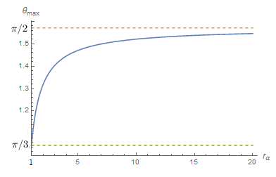
Figure 3: The maximum angle to have a bounce as a function of the anisotropy velocity $r_{\alpha}\in[1,\infty)$. The two limit values $\frac{\pi}{3}\ (r_{\alpha}=1)$ and $\frac{\pi}{2}\ (r_{\alpha}\to\infty)$ are highlited.

Each bounce involves new values for the constants of motion of the free particle ($p_{\pm},H_{\alpha}$) and a change in its direction. The relation between the directions before and after a bounce can be inferred by considering the Hamilton’s equations (58) again, this time with $V_{B}=e^{-8\beta_{+}}$.

First of all we observe that $V_{B}$ depends only from $\beta_{+}$, from which we deduce that $p_{-}$ is yet a constant of motion. A second constant of motion is $K\coloneqq H_{\alpha}-\frac{1}{2}p_{+}$, as we can verify from the Hamilton equations (58). An expression for $p_{\pm}$ can be derived from Eq. (58a):

$$p_{\pm}=\frac{1}{\mu}\beta^{\prime}_{\pm}\sin(\mu H_{\alpha})\sqrt{1-\sin^{2}(\mu H_{\alpha})}$$ (64)

where the compact notation $\sqrt{\mu^{2}(p^{2}+\frac{3(4\pi)^{4}}{\kappa^{2}}e^{4\alpha-8\beta_{+}})}=\\ \sin(\mu H_{\alpha})$ is used. By the substitution of this expression and of the parameterization (62) in the two constants of motion we obtain two modified conservation laws:

$$r_{\alpha_{i}}\sin(\theta_{i})\sin(\mu H_{i})\sqrt{1-\sin^{2}(\mu H_{i})}=\\ =r_{\alpha_{f}}\sin(\theta_{f})\sin(\mu H_{f})\sqrt{1-\sin^{2}(\mu H_{f})}$$ (65a)

$$H_{i}+\frac{1}{2\mu}r_{\alpha_{i}}\cos(\theta_{i})\sin(\mu H_{i})\sqrt{1-\sin^{2}(\mu H_{i})}=\\ =H_{f}-\frac{1}{2\mu}r_{\alpha_{f}}\cos(\theta_{f})\sin(\mu H_{f})\sqrt{1-\sin^{2}(\mu H_{f})}$$ (65b)

The reflection law can be then derived after a series of algebraic passages which involve the substitution of (65a) in (65b), and the use of the explicit expression (59) for the anisotropy velocity $r_{\alpha}$:

$$\frac{1}{2}\mu p_{f}\left(\cos\theta_{f}+\frac{\cos\theta_{i}\sin\theta_{f}}{\sin\theta_{i}}\right)=\\ =\arcsin(\mu p_{f})-\arcsin(\mu p_{i})$$ (66)

In order to have this law in a simpler form, comparable to the standard case, an expansion up to the second order in $\mu p<<1$ is required. The final result is:

$$\frac{1}{2}\sin(\theta_{i}+\theta_{f})=\sin\theta_{i}(1+\Pi_{f}^{2})-\sin\theta_{f}(1+\Pi_{i}^{2})$$ (67)

where we have defined $\Pi^{2}=\frac{1}{6}\mu^{2}p^{2}$.

5.2 Comparison with previous models

As we stressed in Sec. 5.1 our model turns out to be very different from Loop Quantum Cosmology Ashtekar:2006es ; Ashtekar:2009vc , which predicts a Big Bounce-like dynamics. Moreover, if the polymer approach is applied to the anisotropies $\beta_{\pm}$, leaving the volume variable $\alpha$ classical Montani:2013 , a singular but non-chaotic dynamics is recovered.

It should be noted that the polymer approach in the perturbative limit can be interpreted as a modified commutation relation Battisti:2008du :

$$[\hat{q},\hat{p}]=i(1-\mu p^{2})$$ (68)

where $\mu>0$ is the deformation parameter. Another quantization method involving an analogue modified commutation relation is the one deriving by the Generalized Uncertainty Principle (GUP):

$$\Delta q\Delta p\geq\frac{1}{2}(1+s(\Delta p)^{2}+s\innerproduct{p}{p}^{2}),\quad(s>0)$$ (69)

through which a minimal length is introduced and which is linked to the commutation relation:

$$[\hat{q},\hat{p}]=i(1+sp^{2})$$ (70)

In BattistiGUP:2009 the Mixmaster model in the GUP approach (applied to the anisotropy variables $\beta_{\pm}$) is developed and the resulting dynamics is very different from the one deriving by the application of the polymer representation to the same variables Montani:2013 . The GUP Bianchi I anisotropy velocity turns out to be always greater than $1$ ($\beta_{GUP}^{\prime 2}=1+6sp^{2}+9s^{2}p^{4}$) and, in particular, greater than the wall velocity $\beta^{\prime GUP}_{wall}$ (which in this case is different from $\frac{1}{2}$). Moreover the maximum angle of incidence for having a bounce is always greater than $\frac{\pi}{3}$. Therefore the occurrence of a bounce between the $\beta$-particle and the potential walls of Bianchi IX can be deduced. The GUP Bianchi II model is not analytic (no reflection law can be inferred), but some qualitative arguments lead to the conclusion that the deformed Mixmaster model can be considered a chaotic system. In conclusion if we apply the two modified commutation relations to the anisotropy (physical) variables of the system we recover very different behaviors. Instead the polymer applied to the geometrical variable $\alpha$ leads to a dynamics very similar to the GUP one described here: the anisotropy velocity (59) is always greater than $1$ and the maximum incident angle (63) varies in the range $\frac{\pi}{3}<\theta_{max}<\frac{\pi}{2}$, so that the chaotic features of the two models can be compared.

5.3 Quantum Analysis

The modified super-Hamiltonian constraint (56) can be easily quantized by promoting all the variables to operators and by approximating $p_{\alpha}$ through the substitution (55):

$$\left[-\frac{1}{\mu^{2}}\sin^{2}(\mu p_{\alpha})+\hat{p}_{+}^{2}+\hat{p}_{-}^{2}+\right.\\ +\left.\frac{3(4\pi)^{4}}{\kappa^{2}}e^{4\alpha}V_{B}(\hat{\beta}_{\pm})\right]\psi(p_{\alpha},p_{\pm})=0$$ (71)

If we consider the potential walls as perfectly vertical, the motion of the quantum $\beta$-particle boils down to the motion of a free quantum particle with appropriate boundary conditions. The free motion solution is obtained by imposing $V_{B}=0$ as usual, and by separating the variables in the wave function: $\psi(p_{\alpha},p_{\pm})=\chi(p_{\alpha})\phi(p_{\pm})$. It should be noted that, although we can no longer take advantage of the adiabatic approximation (51), due to the necessary use of the momentum polarization in Eq. (71), nonetheless we can suppose that the separation of variables is reasonable. In fact in the limit where the polymer correction vanishes ($\mu\to 0$), the Misner solution (for which the adiabatic hypothesis is true) is recovered.

The anisotropy component $\phi(p_{\pm})$ is obtained by solving the eigenvalues problem:

$$(\hat{p}_{+}^{2}+\hat{p}_{-}^{2})\phi(p_{\pm})=k^{2}\phi(p_{\pm})$$ (72)

where $k^{2}=k_{+}^{2}+k_{-}^{2}$ ($k_{\pm}$ are the eigenvalues of $\hat{p}_{\pm}$ respectively). Therefore the eigenfunctions are
$\phi(p_{\pm})=\phi_{+}(p_{+})\phi_{-}(p_{-})$ with:

$$\phi_{+}(p_{+})=A\delta(p_{+}-k_{+})+B\delta(p_{+}+k_{+})$$ (73a)

$$\phi_{-}(p_{-})=C\delta(p_{-}-k_{-})+D\delta(p_{-}+k_{-})$$ (73b)

where $A,B,C,D$ are integration constants. By substituting this result in (71) we find also the isotropic component $\chi(p_{\alpha})$ and the related eigenvalue $\bar{p}_{\alpha}$:

$$\chi(p_{\alpha})=\delta(p_{\alpha}-\bar{p}_{\alpha})$$ (74)

$$\bar{p}_{\alpha}=\frac{1}{\mu}\arcsin(\mu k)$$ (75)

The potential term is approximated by a square box with vertical walls, whose length is expressed by $L(\alpha)=L_{0}+\alpha$, so that they move outward with velocity $|\beta^{\prime}_{wall}|=\frac{1}{2}$:

$$V_{B}(\alpha,\beta_{\pm})=\begin{cases}0\quad\ \text{if}\quad-\frac{L(\alpha)}{2}\leq\beta_{\pm}\leq\frac{L(\alpha)}{2}\\ \infty\quad\text{elsewhere}\end{cases}$$ (76)

The system is then solved by applying the boundary conditions:

$$\begin{cases}\phi_{+}\left(\frac{L(\alpha)}{2}\right)=\phi_{+}\left(-\frac{L(\alpha)}{2}\right)=0\\ \phi_{-}\left(\frac{L(\alpha)}{2}\right)=\phi_{-}\left(-\frac{L(\alpha)}{2}\right)=0\end{cases}$$ (77)

to the eigenfunctions (73), expressed in coordinate representation (i.e. $\phi(\beta_{\pm})$, which can be calculated through a standard Fourier transformation). The final solution is:

$$\phi_{n,m}(\beta_{\pm})=\frac{1}{2L(\alpha)}\left(e^{ik^{+}_{n}\beta_{+}}-e^{-ik^{+}_{n}\beta_{+}}e^{-in\pi}\right)\cdot\\ \cdot\left(e^{ik^{-}_{m}\beta_{-}}-e^{-ik^{-}_{m}\beta_{-}}e^{-im\pi}\right)$$ (78)

with:

$$k^{+}_{n}=\frac{n\pi}{L(\alpha)};\qquad k^{-}_{m}=\frac{m\pi}{L(\alpha)}$$ (79)

Instead the isotropic component results to be:

$$\bar{p}_{\alpha}=\frac{1}{\mu}\arcsin\left(\frac{\mu\pi}{L(\alpha)}\sqrt{m^{2}+n^{2}}\right)$$ (80)

$$\chi(\alpha)=e^{\frac{i}{\mu}\underset{0}{\overset{x}{\int}}dt\arcsin\left(\frac{\mu\pi}{L(\alpha)}\sqrt{m^{2}+n^{2}}\right)}$$ (81)

We emphasize the fact that, as we announced at the beginning of this section, the Misner solution (53) can be easily recovered from Eq. (80), by taking the limit $\mu\to 0$.

5.4 Adiabatic Invariant

Because of the various hints about the presence of a chaotic behavior, outlined in Sec. 5.1 and that will be confirmed by the analysis of the Poincaré map in Sec 7, we can reproduce a calculation similar to the Misner’s one Misner:1969 in order to obtain information about the quasi-classical properties of the early universe. In Sec. 5.1 we found that the $\beta$-point undergoes an infinite series of bounces against the three potential walls, moving with constant velocity between a bounce and another. Every bounce implies a decreasing of $H_{\alpha}$ due to the conservation of $K=H_{\alpha}-\frac{1}{2}p_{+}$ and the definition of a new direction of motion through Eq. (67). Because of the ergodic properties of the motion we can assume that it won’t be influenced by the choice of the initial conditions. Thus we can choose them in order to simplify the subsequent analysis. A particularly convenient choice is: $\theta_{i}+\theta_{f}=60^{\circ}$ for the first bounce. In fact as a consequence of the geometrical properties of the system all the subsequent bounces will be characterized by the same angle of incidence: $\theta^{\prime}_{i}=\theta_{i}$ (Fig. 4).

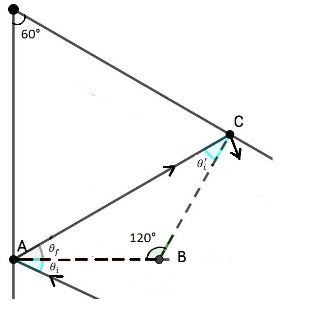
Figure 4: Relation between the angles of incidence of two following bounces: $\theta_{i}$ and $\theta^{\prime}_{i}$. Here we can see that the condition $\theta_{f}+\theta^{\prime}_{i}=60^{\circ}$ must hold in order to have $180^{\circ}$ as the sum of internal angles of the triangle $A\overset{\triangle}{B}C$. It follows that the initial condition $\theta_{i}+\theta_{f}=60^{\circ}$ implies $\theta_{i}=\theta_{i}^{\prime}$ for every couple of subsequent bounces.

Let us now analyze a single bounce, keeping in mind Fig. 5.

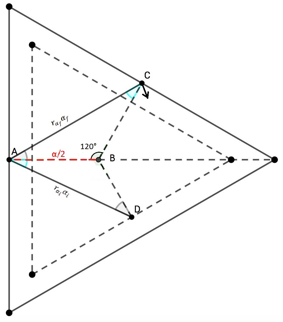
Figure 5: Geometric relations between two successive bounces.

At the time $\alpha$ in which we suppose the bounce to occur, the wall is in the position $\beta_{wall}=\frac{|\alpha|}{2}$. Moving between two walls, the particle has the constant velocity $|\beta^{\prime}|=r_{\alpha}$ (Eq. (59)), so that we can deduce the spatial distance between two bounces in terms of the “time” $|\alpha|$ necessary to cover such a distance:

$$[\text{distance covered before the bounce}]=r_{\alpha_{i}}|\alpha_{i}|$$ (82a)

$$[\text{distance covered after the bounce}]=r_{\alpha_{f}}|\alpha_{f}|$$ (82b)

Now if we apply the Sine theorem to the triangles $A\overset{\triangle}{B}C$ and $A\overset{\triangle}{B}D$, we find the relation:

$$\frac{r_{\alpha_{i}}|\alpha_{i}|}{r_{\alpha_{f}}|\alpha_{f}|}=\frac{\sin\theta_{i}}{\sin\theta_{f}}$$ (83)

Moreover, from (65a) one gets:

$$\frac{r_{\alpha_{f}}\sin(\mu H_{\alpha_{f}})\sqrt{1-\sin^{2}(\mu H_{\alpha_{f}})}}{r_{\alpha_{i}}\sin(\mu H_{\alpha_{i}})\sqrt{1-\sin^{2}(\mu H_{\alpha_{i}})}}=\frac{\sin\theta_{i}}{\sin\theta_{f}}=\text{cost}$$ (84)

From these two relations we can then deduce a quantity which remains unaltered after the bounce:

$$r_{\alpha_{i}}^{2}|\alpha_{i}|\sin(\mu H_{i})\sqrt{1-\sin^{2}(\mu H_{i})}=\\ =r_{\alpha_{f}}^{2}|\alpha_{f}|\sin(\mu H_{f})\sqrt{1-\sin^{2}(\mu H_{f})}$$ (85)

Now we can generalize the argument to the n-th bounce (taking place at the “time” $\alpha_{n}$ instead of $\alpha$). By using again the Sine theorem (applied to the triangle $A\overset{\triangle}{B}D$) we get the relation $r_{\alpha_{i}}|\alpha_{i}|=\frac{\sin 120^{\circ}}{2\sin\theta_{f}}|\alpha_{n}|=C|\alpha_{n}|$, where $C$ takes the same value for every bounce. Correspondingly $r_{\alpha_{f}}|\alpha_{f}|=C|\alpha_{n+1}|$. If we substitute these new relations in Eq. (85),we can then conclude that:

$$\langle r_{\alpha}|\alpha|\sin(\mu H)\sqrt{1-\sin^{2}(\mu H)}\rangle=\text{cost}$$ (86)

where the average value is taken over a large number of bounces. As we are interested in the behavior of quantum states with high occupation number, remembering that for such states the quasi-classical approximation $H_{\alpha}\simeq\bar{p}_{\alpha}$ is valid, we can substitute Eq. (80) and Eq. (59) in (86) and evaluate the correspondent quantity in the limit $\alpha\to-\infty$. The result is that also in this case the occupation number is an adiabatic invariant:

$$\langle\sqrt{m^{2}+n^{2}}\rangle=\text{cost}$$ (87)

that is the same conclusion obtained by Misner without the polymer deformation. It follows that also in this case a quasi-classical state of the Universe is allowed up to the initial singularity.

6 Semiclassical solution for the Bianchi I and II models

As we have already outlined in Sec. 3, to calculate the BKL map it is necessary first to solve the Einstein’s Eqs for the Bianchi I and Bianchi II models.

Therefore, in Sec. 6.1 we solve the Hamilton’s Eqs in Misner variables for the Polymer Bianchi I, in the semiclassical approximation introduced in Sec. 5.1.

Then in Sec. 6.2 we derive a parametrization for the Polymer Kasner indices. It is not possible anymore to parametrize the three Kasner indices using only one parameter $u$ as in (27), but two parameters are needed. This is due to a modification to the Kasner constraint (26).

In Sec. 6.3 we calculate how the Bianchi II Einstein’s Eqs are modified when the PQM is taken into account. Then we derive a solution for these Eqs, using the lowest order perturbation theory in $\mu$. We are therefore assuming that $\mu$ is little with respect to the Universe volume cubic root.

6.1 Polymer Bianchi I

As already shown in Sec. 5.1, the Polymer Bianchi I Hamiltonian is obtained by simply setting $V_{B}=0$ in (56). Upon solving the Hamilton’s Eqs derived from the Hamiltonian (56) in the case of Bianchi I, variables $p_{\alpha}$ and $p_{\pm}$ are recognized to be constants throughout the evolution. We then choose the time gauge so as to have a linear dependence of the volume $\mathcal{V}$ from the time $t$ with unity slope, as in the standard solution (23):

$$N=-\frac{64\pi^{2}\mu}{\kappa\sin(2{\mu}p_{\alpha})}$$ (88)

Moreover, to have a Universe expanding towards positive times, we must restrict the range of $\sin(2{\mu}p_{\alpha})<0$. This condition reflects on $p_{\alpha}$ as

$$-\frac{\pi}{2\mu}+\frac{n\pi}{\mu}<p_{\alpha}<\frac{n\pi}{\mu},\qquad p_{\alpha}\in\mathbb{Z}$$ (89)

The branch connected to the origin $n=0$, will be called connected-branch. For $\mu\rightarrow 0$, it gives the correct continuum limit: $p_{\alpha}<0$. Even though, for different choices of $n\neq 0$, we cannot provide a simple and clear explanation of their physical meaning, when we will define the parametrization of the Kasner indices in Sec. 6.2, we will be forced to consider another branch too, in addition to the connected-one. We choose arbitrarily the $n=1$ branch and, by analogy, we will call it the disconnected-branch.

The solution to Hamilton’s Eqs for Polymer Bianchi I in the (88) time gauge, reads as

$$\alpha(t)= ~{}\frac{1}{3}\ln(t)$$ (90a)

$$\beta_{\pm}(t)= -\frac{2}{3}\frac{\mu p_{\pm}}{\sin(2{\mu}p_{\alpha})}\ln(t)=-\frac{2\mu p_{\pm}}{\sin(2{\mu}p_{\alpha})}\alpha(t)$$ (90b)

Since $p_{\alpha}$, $p_{\pm}$ and $\mu$ in the (90) are all numerical constants, it is qualitatively the very same as the classical solution (23). In particular, even in the Polymer case the volume $\mathcal{V}(t)\propto e^{3\alpha(t)}=t$ goes to zero when $t\rightarrow 0$: i.e. the singularity is not removed and we have a Big Bang, as already pointed out in Sec. 5.1.

By making a reverse canonical transformation from Misner variables ($\alpha$, $\beta_{\pm}$) to ordinary ones ($q_{l}$, $q_{m}$, $q_{n}$), we find out that (24) holds unchanged while (26) is modified into:

$${p_{l}}^{2}+{p_{m}}^{2}+{p_{n}}^{2}=\frac{1}{3}\left(1+\frac{2}{\cos^{2}(\mu p_{\alpha})}\right)$$ (91)

If the continuum limit $\mu\rightarrow 0$ is taken, we get back the old constraint (26) as expected. Since the relation

$${p_{l}}^{2}+{p_{m}}^{2}+{p_{n}}^{2}=\frac{1}{3}+\frac{2}{3}\beta^{\prime 2}$$ (92)

holds, the inequality ${p_{l}}^{2}+{p_{m}}^{2}+{p_{n}}^{2}\geq 1,\quad\forall p_{\alpha}\in\mathbb{R}$ is directly linked to $\beta$-point velocity (59) being always equal or greater than one, as demonstrated in Sec. 5.1. This is a noteworthy difference with respect to the standard case of Eq. (45), where the speed was always one.

We can derive an alternative expression for the Kasner constraint (91) by exploiting the notation of Eqs (23):

$${p_{l}}^{2}+{p_{m}}^{2}+{p_{n}}^{2}=\frac{1}{3}\left(1+\frac{4}{1\pm\sqrt{1-Q^{2}}}\right)$$ (93)

where the plus sign is for the connected-branch while the minus for the disconnected-branch. We have defined the dimensionless quantity $Q$ as

$$Q:=\frac{{(8\pi)}^{2}\mu\Lambda}{\kappa}$$ (94)

It is worth noticing that the lattice spacing $\mu$ has been incorporated in $Q$, so that the continuum limit $\mu\to 0$ is now equivalently reached when $Q\to 0$. Condition (89) reflects on the allowed range for Q:

$$\absolutevalue*{Q}\leq 1$$ (95)

both for the connected and disconnected branches.

6.2 Parametrization of the Kasner indices

In this Section we define a parametrization of the Polymer Kasner indices. In the standard case of (27), because there are three Kasner indices and two Kasner constraints (24) and (26), only one parameter $u$ is needed to parametrize the Kasner indices. On the other hand, in the Polymer case, even if there are two Kasner constraints (24) and (93) as well, constraint (93) already depends on another parameter $Q$. This means that any parametrization of the Polymer Kasner indices will inevitably depend on two parameters, that we arbitrarily choose as $u$ and $Q$, where $u$ is defined on the same range as the standard case (27) and $Q$ was defined in (94). They are both dimensionless. We will refer to the following expressions as the $(u,Q)$-parametrization for the Polymer Kasner indices:

$$\begin{split}p_{1}&=\frac{1}{3}\left\{1-\frac{1+4u+u^{2}}{1+u+u^{2}}{\left[\frac{1}{2}\left(1\pm\sqrt{1-Q^{2}}\right)\right]}^{-\frac{1}{2}}\right\}\\ p_{2}&=\frac{1}{3}\left\{1+\frac{2+2u-u^{2}}{1+u+u^{2}}{\left[\frac{1}{2}\left(1\pm\sqrt{1-Q^{2}}\right)\right]}^{-\frac{1}{2}}\right\}\\ p_{3}&=\frac{1}{3}\left\{1+\frac{-1+2u+2u^{2}}{1+u+u^{2}}{\left[\frac{1}{2}\left(1\pm\sqrt{1-Q^{2}}\right)\right]}^{-\frac{1}{2}}\right\}\end{split}$$ (96)

where the plus sign is for the connected branch and the minus sign is for the disconnected branch. By construction, the standard $u$-parametrization (27) is recovered in the limit $Q\rightarrow 0$ of the connected branch. We will see clearly in Sec. 7.2 how the $Q$ parameter can be thought of as a measure of the quantization degree of the Universe. The more the $Q$ of the connected-branch is big in absolute value, the more the deviations from the standard dynamics due to PQM are pronounced. The opposite is true for the disconnected-branch. To gain insight on multiple-parameters parametrizations of the Kasner indices, the reader can refer toMontani:2004mq ; Elskens:1987 .

The $(u,Q)$-parametrization (96) is even in $Q$: $p_{a}(u,Q)=p_{a}(u,-Q)$ with $a=l,m,n$. We can thus assume without loss of generality that $0\leq Q\leq 1$. Another interesting feature of the Polymer Bianchi I model, that is evident from Fig. 6, is that, for every $u$ and $Q$ in a non-null measure set, two Kasner indices can be simultaneously negative (instead of only one as is the case of the standard $u$-parametrization (27)).

In a similar fashion as the $u$ parameter is “remapped” in the standard case (second line of (39)), also the $(u,Q)$ parametrization is to be “remapped”, if the $u$ parameter happens to become less than one. Down below we list these remapping prescriptions explicitly: we show how the $(u,Q)$-parametrization (96) can be recovered if the $u$ parameter becomes smaller than 1, through a reordering of the Kasner indices and a remapping of the $u$ parameter.

• $0<u<1$

  $$\begin{dcases}p_{1}\left(u,Q\right)\rightarrow p_{1}\left(\frac{1}{u},Q\right)\\ p_{2}\left(u,Q\right)\rightarrow p_{3}\left(\frac{1}{u},Q\right)\\ p_{3}\left(u,Q\right)\rightarrow p_{2}\left(\frac{1}{u},Q\right)\end{dcases}$$

• $-\tfrac{1}{2}<u<0$

  $$\begin{dcases}p_{1}\left(u,Q\right)\rightarrow p_{2}\left(-\frac{1+u}{u},Q\right)\\ p_{2}\left(u,Q\right)\rightarrow p_{3}\left(-\frac{1+u}{u},Q\right)\\ p_{3}\left(u,Q\right)\rightarrow p_{1}\left(-\frac{1+u}{u},Q\right)\end{dcases}$$

• $-1<u<-\frac{1}{2}$

  $$\begin{dcases}p_{1}\left(u,Q\right)\rightarrow p_{3}\left(-\frac{u}{1+u},Q\right)\\ p_{2}\left(u,Q\right)\rightarrow p_{2}\left(-\frac{u}{1+u},Q\right)\\ p_{3}\left(u,Q\right)\rightarrow p_{1}\left(-\frac{u}{1+u},Q\right)\end{dcases}$$

• $-2<u<-1$

  $$\begin{dcases}p_{1}\left(u,Q\right)\rightarrow p_{3}\left(-\frac{1}{1+u},Q\right)\\ p_{2}\left(u,Q\right)\rightarrow p_{1}\left(-\frac{1}{1+u},Q\right)\\ p_{3}\left(u,Q\right)\rightarrow p_{2}\left(-\frac{1}{1+u},Q\right)\end{dcases}$$

• $u<-2$

  $$\begin{dcases}p_{1}\left(u,Q\right)\rightarrow p_{2}\left(-\left(1+u\right),Q\right)\\ p_{2}\left(u,Q\right)\rightarrow p_{1}\left(-\left(1+u\right),Q\right)\\ p_{3}\left(u,Q\right)\rightarrow p_{3}\left(-\left(1+u\right),Q\right)\end{dcases}$$

where the indices on the left are defined for the $u$ shown after the bullet $\bullet$, while the indices on the right are in the “correct” range $u>1$. The arrow ‘$\rightarrow$’ is there to indicate a conceptual mapping. However, in value it reads as an equality ‘$=$’. As far as the Q parameter is concerned, a “remapping” prescription for $Q$ is not needed because values outside the boundaries (95) are not physical and should never be considered.

In Figure 6 the values of the ordered Kasner indices are displayed for the $(u,Q)$-parametrization (96), where $Q\in\left[0,1\right]$. Because the range $u>1$ is not easily plottable, the equivalent parametrization in $u\in\left[0,1\right]$ was used. We notice that the roles of $p_{m}$ and $p_{n}$ are exchanged for this range choice.

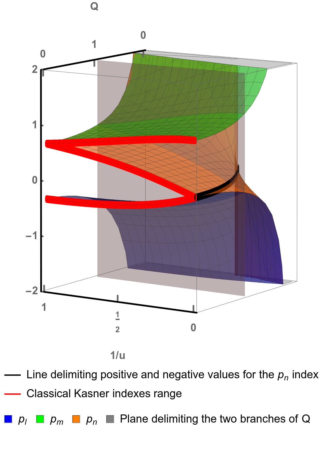
Figure 6: Plot of the “spectrum” of the Kasner indices in the $(u,Q)$-parametrization (96). Every value of $(u,Q)$ in the dominion $u\in[1,\infty)$ and $Q\in[0,1]$ uniquely selects a triplet of Kasner indices. The vertical plane delimits the two branches of the $(u,Q)$-parametrization (96). The connected-branch is the one containing the red (dark gray) lines, i.e. the standard parametrization shown in Fig. 1. The $Q$ parameter of the connected-branch is increasing from 0 to 1 in the positive direction of the $Q$-axis, while for the disconnected-branch it is decreasing from 1 to 0. The black line delimits the part of the $(u,Q)$-plane where there is only one (above) or two (below) negative Kasner indices. The plot is cut on the bottom and on top but it is actually extending up to $\pm\infty$.

6.3 Polymer Bianchi II

Here we apply the method described in 6.1 to find an approximate solution to the Einstein’s Eqs of the Polymer Bianchi II model. We start by selecting the $V_{B}$ potential appropriate for Bianchi II (60) and we substitute it in the Hamiltonian (56) (in the following we will always assume the time gauge $N=1$).

Then, starting from Hamilton’s Eqs, inverting the Misner canonical transformation and converting the synchronous time $t$-derivatives into logarithmic time $\tau$-derivatives, the Polymer Bianchi II Einstein’s Eqs are found to be:

$$\begin{dcases}{q_{l}}_{\tau\tau}(\tau)=\frac{1}{3}e^{2q_{l}(\tau)}\left[-4+\sqrt{1+{\left(\frac{2{(4\pi)}^{2}\mu}{\kappa}v(\tau)\right)}^{2}}\right]\\ {q_{m}}_{\tau\tau}(\tau)=\frac{1}{3}e^{2q_{l}(\tau)}\left[2+\sqrt{1+{\left(\frac{2{(4\pi)}^{2}\mu}{\kappa}v(\tau)\right)}^{2}}\right]\\ {q_{n}}_{\tau\tau}(\tau)=\frac{1}{3}e^{2q_{l}(\tau)}\left[2+\sqrt{1+{\left(\frac{2{(4\pi)}^{2}\mu}{\kappa}v(\tau)\right)}^{2}}\right]\end{dcases}$$ (97)

where $v(\tau):={q_{l}}_{\tau}(\tau)+{q_{m}}_{\tau}(\tau)+{q_{n}}_{\tau}(\tau)$. In the $Q\ll 1$ approximation it is enough to consider only the connected-branch of the solutions, i.e. the branch that in the limit $\mu\to 0$ make Eqs (97) reduce to the correct classical Eqs (29).

Now we find an approximate solution to the system (97), with the only assumption that $\mu$ is little compared to the cubic root of the Universe volume. We are entitled then to exploit the standard perturbation theory and expand the solution until the first non-zero order in $\mu$. Because $\mu$ appears only squared $\mu^{2}$ in the Einstein’s Eqs (97), the perturbative expansion will only contain even powers of $\mu$.

First we expand the solution at the first order in $\mu^{2}$

$$\begin{dcases}q_{l}(\tau)=q_{l}^{0}(\tau)+\mu^{2}q_{l}^{1}(\tau)+O(\mu^{4})\\ q_{m}(\tau)=q_{m}^{0}(\tau)+\mu^{2}q_{m}^{1}(\tau)+O(\mu^{4})\\ q_{n}(\tau)=q_{n}^{0}(\tau)+\mu^{2}q_{n}^{1}(\tau)+O(\mu^{4})\end{dcases}$$ (98)

where $q_{l,m,n}^{0}$ are the zeroth order terms and $q_{l,m,n}^{1}$ are the first order terms in $\mu^{2}$. We recall the zeroth order solution $q_{l,m,n}^{0}$ is just the classical solution (31), where the $q_{l,m,n}(\tau)$ there must be now appended a 0-apex, accordingly.

Considering the fact that ${q_{m}}_{\tau\tau}={q_{n}}_{\tau\tau}$, we can simplify $q_{n}(\tau)$ from (97), by setting

$$q_{n}(\tau)=q_{m}(\tau)+2(c_{5}+c_{6}\tau)+\mu^{2}(c_{11}+c_{12}\tau)+\\ -2(c_{3}+c_{4}\tau)-\mu^{2}(c_{9}+c_{10}\tau)$$ (99)

where the first six constants of integration $c_{1},c_{2},\dots,c_{6}$ play the same role at the zeroth order as in Eq. (31), while the successive six $c_{7},\dots,c_{12}$ are needed to parametrize the first order solution.

Then we substitute (99) in (97) and, as it is required by perturbations theory, we gather only the zeroth and first order terms in $\mu^{2}$ and neglect all the higher order terms. The Einstein’s Eqs for the first order terms $q_{l}^{1}$ and $q_{m}^{1}$ are then found to be:

$$\frac{\partial^{2}{q_{l}^{1}}}{\partial\tau^{2}}+{c_{1}}^{2}\sech^{2}(c_{1}\tau+c_{2})\times$$ (100)

$$\times\left\{2{q_{l}^{1}}+\frac{C}{3}{\left[2(c_{6}+c_{4})+c_{1}\tanh(c_{1}\tau+c_{2})\right]}^{2}\right\}=0$$

$$\frac{\partial^{2}{q_{m}^{1}}}{\partial\tau^{2}}+{c_{1}}^{2}\sech^{2}(c_{1}\tau+c_{2})\times$$ (101)

$$\times\left\{2{q_{l}^{1}}+\frac{C}{3}{\left[2(c_{6}+c_{4})+c_{1}\tanh(c_{1}\tau+c_{2})\right]}^{2}\right\}=0$$

where we have defined $C\equiv\frac{2{(4\pi)}^{2}}{\kappa^{2}}$ for brevity and we have substituted the zeroth order solution (31) where needed.

Eqs (6.3) are two almost uncoupled non-homogeneous ODEs. (100) is a linear second order non-homogeneous ODE with non-constant coefficients and, being completely uncoupled, it can be solved straightly. (101) is solved by mere substitution of the solution of (100) in it and subsequent double integration.

To solve (100) we exploited a standard method that can be found, for example, in (Tenenbaum:2012, , Lesson 23). This method is called reduction of order method and, in the case of a second order ODE, can be used to find a particular solution once any non trivial solution of the related homogeneous equation is known.

The homogeneous equation associated to (100) is

$$\frac{\partial^{2}{q_{l}^{1}}}{\partial\tau^{2}}+2{c_{1}}^{2}\sech^{2}(c_{1}\tau+c_{2}){q_{l}^{1}}=0$$ (102)

whose general solution reads as:

$${q_{l}^{1}}_{O}(\tau)=-\frac{c_{8}}{c_{1}}+(c_{7}+c_{8}\tau)\tanh(c_{1}\tau+c_{2})$$ (103)

By applying the above-mentioned method, we obtain the following solution for (100)

$$\begin{split}q_{l}^{1}(\tau)=&-\tfrac{c_{8}}{c_{1}}+(c_{7}+c_{8}\tau)\tanh(c_{1}\tau+c_{2})\\ &-\tfrac{C}{36}c_{1}\tanh(c_{1}\tau+c_{2})\left\{3\left[{c_{1}}^{2}+8{(c_{4}+c_{6})}^{2}\right]\tau\right.\\ &+16(c_{4}+c_{6})\ln\left[\cosh(c_{1}\tau+c_{2})\right]-3c_{1}\tanh(c_{1}\tau+c_{2})\Big{\}}\end{split}$$ (104)

The solution for (101) is found by substituting (104) in it and then integrating two times:

$$\begin{split}q_{m}^{1}(\tau)=&~{}c_{10}+c_{9}\tau-(c_{7}+c_{8}\tau)\tanh(c_{1}\tau+c_{2})\\ &-\tfrac{C}{36}\Big{\{}16c_{1}(c_{4}+c_{6})(c_{1}\tau+c_{2}){c_{1}}^{2}\sech^{2}(c_{1}\tau+c_{2})\\ &+8\left[{c_{1}}^{2}+12{(c_{4}+c_{6})}^{2}\right]\ln(\cosh(c_{1}\tau+c_{2}))\\ &-c_{1}\tanh(c_{1}\tau+c_{2})\left[48(c_{4}+c_{6})+3\left({c_{1}}^{2}+8{(c_{4}+c_{6})}^{2}\right)\tau\right.\\ &+16(c_{4}+c_{6})\ln(\cosh(c_{1}\tau+c_{2}))\Big{]}\Big{\}}\end{split}$$ (105)

Now that we know $q_{l}^{0}$, $q_{l}^{1}$, $q_{m}^{0}$ and $q_{m}^{1}$, the complete solution for $q_{l}$, $q_{m}$ and $q_{n}$ is found through (98) and (99) by mere substitution.

7 Polymer BKL map

In this last Section, we calculate the Polymer modified BKL map and study some of its properties.

In Sec. 7.1 the Polymer BKL map on the Kasner indices is derived while in Sec. 7.2 some noteworthy properties of the map are discussed.

Finally in Sec 7.3 the results of a simple numerical simulation of the Polymer BKL map over many iterations are presented and discussed.

7.1 Polymer BKL map on the Kasner indices

Here we use the method outlined in Secs. from 6.1 to 6.3 to directly calculate the Polymer BKL map on the Kasner indices.

First, we look at the asymptotic limit at $\pm\infty$ for the solution of Polymer Bianchi II (98). As in the standard case, the Polymer Bianchi II model “links together” two Kasner epochs at plus and minus infinity. In this sense, the dynamics of Polymer Bianchi II is not qualitatively different from the standard one. We will tell the quantities at plus and minus infinity apart by adding a prime $\Box^{\prime}$ to the quantities at minus infinity and leaving the quantities at plus infinity un-primed. The two Kasner solutions at plus and minus infinity can be still parametrized according to (23).

By summing together equations (23) and using the first Kasner constraint (24), we find that:

$$\begin{cases}\lim_{\tau\rightarrow+\infty}\frac{1}{2\tau}\left(q_{l}+q_{m}+q_{n}\right)=\Lambda\\ \lim_{\tau\rightarrow-\infty}\frac{1}{2\tau}\left(q^{\prime}_{l}+q^{\prime}_{m}+q^{\prime}_{n}\right)=\Lambda^{\prime}\end{cases}$$ (106)

By taking the limits at $\tau\rightarrow\pm\infty$ of the derivatives of the Polymer Bianchi II solution (98),
 
$\boxed{\lim_{\tau\rightarrow+\infty}}$

$${q_{l}}_{\tau}= -c_{1}+\mu^{2}c_{8}-\mu^{2}\frac{C}{36}c_{1}\left[3{c_{1}}^{2}+16c_{1}(c_{4}+c_{6})+24{(c_{4}+c_{6})}^{2}\right]$$

$${q_{m}}_{\tau}= ~{}2c_{4}+c_{1}+\mu^{2}(-c_{8}+c_{9})-\mu^{2}\frac{C}{36}c_{1}\left[5{c_{1}}^{2}+24{(c_{4}+c_{6})}^{2}\right]$$

$${q_{n}}_{\tau}= ~{}2c_{6}+c_{1}+\mu^{2}(-c_{8}+c_{11})-\mu^{2}\frac{C}{36}c_{1}\left[5{c_{1}}^{2}+24{(c_{4}+c_{6})}^{2}\right]$$

$$\Lambda= ~{}\frac{c_{1}}{2}+c_{4}+c_{6}+\mu^{2}\frac{1}{2}(-c_{8}+c_{9}+c_{11})+$$

$$~{}-\mu^{2}\frac{C}{72}c_{1}\left[13{c_{1}}^{2}+16c_{1}(c_{4}+c_{6})+168{(c_{4}+c_{6})}^{2}\right]$$ (107)

$\boxed{\lim_{\tau\rightarrow-\infty}}$

$${q^{\prime}_{l}}_{\tau}= ~{}c_{1}-\mu^{2}c_{8}+\mu^{2}\frac{C}{36}c_{1}\left[3{c_{1}}^{2}-16c_{1}(c_{4}+c_{6})+24{(c_{4}+c_{6})}^{2}\right]$$

$${q^{\prime}_{m}}_{\tau}= ~{}2c_{4}-c_{1}-\mu^{2}(c_{8}+c_{9})+\mu^{2}\frac{C}{36}c_{1}\left[5{c_{1}}^{2}+24{(c_{4}+c_{6})}^{2}\right]$$

$${q^{\prime}_{n}}_{\tau}= ~{}2c_{6}-c_{1}-\mu^{2}(c_{8}+c_{11})+\mu^{2}\frac{C}{36}c_{1}\left[5{c_{1}}^{2}+24{(c_{4}+c_{6})}^{2}\right]$$

$$\Lambda^{\prime}= ~{}-\frac{c_{1}}{2}+c_{4}+c_{6}+\mu^{2}\frac{1}{2}(c_{8}+c_{9}+c_{11})+$$

$$~{}+\mu^{2}\frac{C}{72}c_{1}\left[13{c_{1}}^{2}-16c_{1}(c_{4}+c_{6})+168{(c_{4}+c_{6})}^{2}\right]$$ (108)

and comparing (107) and (108) with (23) and (106), we can find the following expressions for the primed and unprimed Kasner indices and $\Lambda$:

$$2\Lambda{p_{l}}=f_{l}(\boldsymbol{c})$$ (109)

$$2\Lambda{p_{m}}=f_{m}(\boldsymbol{c})$$ (110)

$$2\Lambda{p_{n}}=f_{n}(\boldsymbol{c})$$ (111)

$$\Lambda=f_{\Lambda}(\boldsymbol{c})$$ (112)

$$2\Lambda^{\prime}{p^{\prime}_{l}}=f^{\prime}_{l}(\boldsymbol{c})$$ (113)

$$2\Lambda^{\prime}{p^{\prime}_{m}}=f^{\prime}_{m}(\boldsymbol{c})$$ (114)

$$2\Lambda^{\prime}{p^{\prime}_{n}}=f^{\prime}_{n}(\boldsymbol{c})$$ (115)

$$\Lambda^{\prime}=f^{\prime}_{\Lambda}(\boldsymbol{c})$$ (116)

where the functions $f_{l,m,n,\Lambda}$ and $f^{\prime}_{l,m,n,\Lambda}$ correspond to the r.h.s. of (107) and (108) respectively and $\boldsymbol{c}$ is a shorthand for the set $\{c_{1},\dots,c_{12}\}$.

Now, in complete analogy with (35), we look for an asymptotic condition. We don’t need to solve the whole system (116), but only to find a relation between the old and new Kasner indices and $\Lambda$ at the first order in $\mu^{2}$. In practice, not all of the (116) relations are actually needed to find an asymptotic condition.

We recall from (36) that the standard BKL map on $\Lambda$ is

$$\Lambda^{\prime}=(1+2p_{l})\Lambda$$ (117)

where we have assumed that $p_{l}<0$, as we will continue to do in the following. As everything until now is hinting to, we prescribe that the Polymer modified BKL map reduces to the standard BKL map when $\mu\to 0$, so that relation (117) is modified in the Polymer case only perturbatively. Since we are considering only the first order in $\mu^{2}$, we can write for the Polymer case:

$$\Lambda^{\prime}=(1+2p_{l})\Lambda+\mu^{2}h(\boldsymbol{c})+O(\mu^{4})$$ (118)

Solving for $h(\boldsymbol{c})$, we find that

$$h(\boldsymbol{c}) =\frac{1}{\mu^{2}}\left(\Lambda^{\prime}-\Lambda-2p_{l}\Lambda\right)$$

$$=\frac{1}{\mu^{2}}\left(f^{\prime}_{\Lambda}(\boldsymbol{c})-f_{\Lambda}(\boldsymbol{c})-f_{l}(\boldsymbol{c})\right)$$

$$=\frac{4C}{9}c_{1}\left[{c_{1}}^{2}+c_{1}(c_{4}+c_{6})+12{(c_{4}+c_{6})}^{2}\right]$$

We can invert the subsystem made up by the zeroth order of equations (113),  (114) and (116)

$$\begin{dcases}2\Lambda{p_{l}}=-c_{1}\\ 2\Lambda{p_{m}}=2c_{4}+c_{1}\\ \Lambda=\frac{c_{1}}{2}+c_{4}+c_{6}\end{dcases}$$

to express $h=h(p_{l},p_{m},\Lambda)$. Finally the asymptotic condition reads as:

$$\Lambda^{\prime}\approx(1+2p_{l})\Lambda-\mu^{2}\frac{16C}{9}{\Lambda}^{3}p_{l}\left(6+11p_{l}+7{p_{l}}^{2}\right)$$ (119)

We stress that this is only one out of many equivalent ways to extract from the system (116) an asymptotic condition.

Now, we need other three conditions to derive the Polymer BKL map. One is provided by the sum of the primed Kasner indices at minus infinity. This is the very same both in the standard case (24) and in the Polymer case.

Sadly, the two conditions (33) and (34) are not valid anymore. Instead, one condition can be derived by noticing that

$${q_{m}}_{\tau\tau}-{q_{n}}_{\tau\tau}=0~{}~{}\Rightarrow~{}~{}{q_{m}}_{\tau}-{q_{n}}_{\tau}=\text{const}~{}~{}\Rightarrow~{}~{}$$

$$({q_{m}}_{\tau}-{q_{n}}_{\tau})|_{\tau\rightarrow+\infty}=({q_{m}}_{\tau}-{q_{n}}_{\tau})|_{\tau\rightarrow-\infty}~{}~{}\Rightarrow~{}~{}$$

$$\Lambda(p_{l}-p_{m})=\Lambda^{\prime}(p^{\prime}_{l}-p^{\prime}_{m})$$

Lastly, we choose as the fourth condition the sum of the squares of the Kasner indices at minus infinity (93). Because of the assumption $Q\ll 1$, we will consider here only the connected branch of (93). We gather now all the four conditions and put them in a system:

$$\begin{dcases}p^{\prime}_{l}+p^{\prime}_{m}+p^{\prime}_{n}=1\\ Q(p_{l}-p_{m})=Q^{\prime}(p^{\prime}_{l}-p^{\prime}_{m})\\ Q^{\prime}\approx(1+2p_{l})Q-\tfrac{2}{9}Q^{3}p_{l}\left(6+11p_{l}+7{p_{l}}^{2}\right)\\ {p^{\prime}_{l}}^{2}+{p^{\prime}_{m}}^{2}+{p^{\prime}_{n}}^{2}=\frac{1}{3}\left(1+\frac{4}{1+\sqrt{1-Q^{2}}}\right)\end{dcases}$$ (120)

where we have also used definition (94).

Finding the polymer BKL map is now only a matter of solving the system (120) for the un-primed indices. The Polymer BKL map at the first order in $\mu^{2}$ is then:

$$\begin{split}p^{\prime}_{l}&\approx-\frac{p_{l}}{1+2p_{l}}-\frac{2}{9}Q^{2}\left[\frac{7+14p_{l}+9{p_{l}}^{2}}{{(1+2p_{l})}^{2}}\right]\\ p^{\prime}_{m}&\approx\frac{2p_{l}+p_{m}}{1+2p_{l}}+\frac{2}{9}Q^{2}p_{l}\times\\ &\times\left[\frac{-3+p_{l}+9{p_{l}}^{2}+8{p_{l}}^{3}+p_{m}\left(6+11p_{l}+7{p_{l}}^{2}\right)}{{(1+2p_{l})}^{2}}\right]\\ p^{\prime}_{n}&\approx\frac{2p_{l}+p_{n}}{1+2p_{l}}+\frac{2}{9}Q^{2}p_{l}\times\\ &\times\left[\frac{-3+p_{l}+9{p_{l}}^{2}+8{p_{l}}^{3}+p_{n}\left(6+11p_{l}+7{p_{l}}^{2}\right)}{{(1+2p_{l})}^{2}}\right]\\ Q^{\prime}&\approx(1+2p_{l})Q-\tfrac{2}{9}Q^{3}p_{l}\left(6+11p_{l}+7{p_{l}}^{2}\right)\\ \end{split}$$ (121)

where all the terms of order $O(Q^{4})$ were neglected. It is worth noticing that, by taking the limit $\mu\rightarrow 0$, the standard BKL map (36) is immediately recovered. We stress that the form of the map is not unique. One can use the two Kasner constraints (24) and (93) to “rearrange” the Kasner indices as needed.

7.2 BKL map properties

First we derive how the Polymer BKL map can be expressed in terms of the $u$ and $Q$ parameters:

$$\begin{dcases}u\\ Q\end{dcases}\xrightarrow[\text{map}]{\text{BKL}}\begin{dcases}u^{\prime}=u^{\prime}(u,Q)\\ Q^{\prime}=Q^{\prime}(u,Q)\\ \end{dcases}$$ (122)

Then we discuss some of its noteworthy properties.

We start by inserting in the polymer BKL map (121) the connected branch of the $(u,Q)$ parametrization (96) and requiring the relations

$$\begin{dcases}p_{l}=p_{1}(u,Q)\\ p_{m}=p_{2}(u,Q)\\ p_{n}=p_{3}(u,Q)\end{dcases}\xrightarrow[\text{map}]{\text{BKL}}\begin{dcases}p^{\prime}_{l}=p_{2}(u^{\prime}(u,Q),Q^{\prime}(u,Q))\\ p^{\prime}_{m}=p_{1}(u^{\prime}(u,Q),Q^{\prime}(u,Q))\\ p^{\prime}_{n}=p_{3}(u^{\prime}(u,Q),Q^{\prime}(u,Q))\end{dcases}$$ (123)

to be always satisfied. The resulting Polymer BKL map on $(u,Q)$ is quite complex. We therefore split it in many terms:

$$A(u)= ~{}72u{\left(u^{2}+u+1\right)}^{2}\left(-2+3u-3u^{2}+u^{3}\right)$$

$$B(u)= ~{}-12-6u+53u^{2}-119u^{3}+204u^{4}+$$

$$~{}-187u^{5}+112u^{6}-57u^{7}+3u^{8}$$

$$C(u)= ~{}5184{(1+u^{2}+u^{4})}^{4}$$

$$D(u)= ~{}1296{(1-u+u^{2})}^{6}{(1+u+u^{2})}^{2}$$

$$E(u)= ~{}3{(1-u+u^{2})}^{2}\left(63-162u+663u^{2}-1350u^{3}+\right.$$

$$~{}+2398u^{4}-3402u^{5}+3607u^{6}-3402u^{7}+$$

$$\left.+2398u^{8}-1350u^{9}+663u^{10}-162u^{11}+63u^{12}\right)$$

$$F(u)= ~{}72(-1+u+3u^{3}+3u^{5}+u^{6}+2u^{7})$$

$$G(u)= ~{}-3+57u-112u^{2}+187u^{3}-204u^{4}+$$

$$~{}+119u^{5}-53u^{6}+6u^{7}+12u^{8}$$

$$H(u)= ~{}-72{(1+u^{2}+u^{4})}^{2}$$

$$L(u)= ~{}3\left(1+u^{2}+u^{4}\right)$$

that have to be inserted in

$$u^{\prime} =\frac{A(u)+Q^{2}B(u)+\sqrt{C(u)+Q^{2}D(u)+Q^{4}E(u)}}{F(u)+Q^{2}G(u)}$$ (124a)

$$Q^{\prime} =\frac{\sqrt{H(u)+\sqrt{C(u)+Q^{2}D(u)+Q^{4}E(u)}}}{L(u)}$$ (124b)

where we recall that the dominions of definition for $u$ and $Q$ are $u\in[1,\infty)$ and $Q\in[0,1]$. All the square-roots and denominators appearing in (124) are well behaved (always with positive argument or non zero respectively) for any $(u,Q)$ in the intervals of definition. It is not clearly evident at first sight, but the polymer BKL map reduces to the standard one (39) if $Q\rightarrow 0$.

Now, we study the asymptotic behavior of the polymer BKL map (124a) for $u$ going to infinity. This limit is relevant to us for two reasons. Firstly, In Sec. 5.1 we already pointed out that infinitely many bounces of the $\beta$-point against the potential walls happen until the singularity is reached. This means that the Polymer BKL map is to be iterated infinitely many times.

Secondly, we suppose the Polymer BKL map (or at least its $u$ portion (124a)) to be ergotic, so that every open set of the parameter space is visited with non null probability. This assumption is backed up by the observation that the Polymer BKL map (124a) tends asymptotically to the standard BKL map (39) (that is ergodic), as shown in the following Sec. 7.3 through a numerical simulation.

Hence, every open interval of the $u>1$ line is to be visited eventually: we want therefore to assess how the map behaves for $u\to\infty$. Physically, a big value for $u$ means a long (in term of epochs) Kasner era, and in turn this means that the Universe is going deep inside one of the corners of Fig. 2. As we can appreciate from Fig. 7, for $u\rightarrow\infty$, $u^{\prime}$ reaches a plateau:

$$\lim_{u\rightarrow\infty}u^{\prime}(u,Q)=\frac{24+Q^{2}+\sqrt{3\left(7Q^{4}+48Q^{2}+192\right)}}{4Q^{2}}$$ (125)

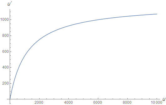
Figure 7: The Polymer BKL map for $u$ (124a) is plotted for $Q=1/10$. There a plateau $u^{\prime}\approx 1200$ is reached at about $u\approx 10^{4}$. This means that for any $u\gtrsim 10^{4}$ the next $u^{\prime}$ will inevitably be $u^{\prime}\approx 1200$, no matter how big $u$ is.

The plateau (125) is higher and steeper the more $Q$ is close to zero. This physically means that there is a sort of “centripetal potential” that is driving the $\beta$-point off the corners and towards the center of the triangle. We infer that this “centripetal potential” is somehow linked to the velocity-like quantity $v(\tau)$ that appears in the polymer Bianchi II Einstein’s Eqs (97). Because of this plateau, the mechanism that drives the Universe away from the corner, implicit in the standard BKL map (39), seems to be much more efficient in the quantum case. For $Q\rightarrow 0$, the plateau tends to disappear: $\lim_{\begin{subarray}{c}u\rightarrow\infty\\ Q\rightarrow 0\end{subarray}}u^{\prime}(u,Q)=\infty$.

As a side note, we remember that it has not been proved analytically that the standard BKL map is still valid deep inside the corners. As a matter of fact, the BKL map can be derived analytically only for the very center of the edges of the triangle of Fig. 2, because those are the only points where the Bianchi IX potential is exactly equal to the Bianchi II potential. The farther we depart from the center of the edges, the more the map looses precision. At any rate, there are some numerical studies for the Bianchi IX model Moser:1973 ; Berger:2002 that show how the standard BKL map is valid with good approximation even inside the corners.

The analysis of the behavior of the Polymer BKL map for the $Q$ parameter (124b) is more convoluted. Little can be said analytically about the overall behavior across multiple iterations because of its evident complexity. For this reason, in Sec. 7.3 we discuss the results of a simple numerical simulation that probes the behavior of the map (124) over many iterations.

The most important point to check is if the dominion of definition (95) for $Q$ is preserved by the map. We remember that for $Q\approx 1$ the perturbation theory, by the means of which we have derived the map, is not valid anymore. So every result in that range is to be taken with a grain of salt.

In Fig. 8 it is shown the maximum value of $u^{*}=u^{*}(Q)$ for which the polymer BKL map on $Q$ is monotonically decreasing, i.e. for any $Q\in[0,1]$ it is shown the corresponding $u^{*}$, such that for $u<u^{*}$ the polymer BKL map on $Q$ is monotonically decreasing. It is clear how the more $Q$ is little the more $u$ can grow before coming to the point that $Q$ stops decreasing and starts increasing.

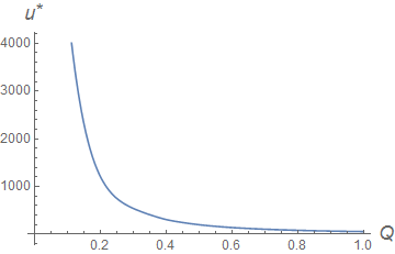
Figure 8: For any $Q\in[0,1]$ it is shown the corresponding $u^{*}(Q)$ such that for $u<u^{*}$ the Polymer BKL map on $Q$ (124b) is monotonically decreasing. For a single iteraction it can be shown that for every $Q<0.96$ the following $Q^{\prime}<1$. The function $u^{*}(Q)$ cannot be given in closed form.

That said, as soon as we consider the behavior of $u$, and particularly the plateau of Fig. 7, we notice that the Universe cannot “indulge” much time in “big-$u$ regions”: even if it happens to assume a huge value for $u$, this is immediately dampened to a much smaller value at the next iteration. The net result is that $Q$ is almost always decreasing as it is also strongly suggested by the numerical simulation of Sec. 7.3.

Summarizing, the Polymer BKL map on $Q$ (124b), apart from a small set of initial conditions in the region where the perturbation theory is failing $Q\approx 1$, preserves the dominion of definition of $Q$ (95) and is decreasing at almost any iteration.

7.3 Numerical simulation

In this Section we present the results of a simple numerical simulation that unveils some interesting features of the Polymer BKL map (124). The main points of this simulation are very simple:

• An initial couple of values for $(u,Q)$ is chosen inside the dominion $u\in[1,\infty)$ and $Q\in[0,0.96]$.

• We remember from Sec.3.3 and 6.2 that, at the end of each Kasner era, the $u$ parameter becomes smaller than 1 and needs to be remapped to values greater than 1. This marks the beginning of a new Kasner era. This remapping is performed through the relations listed on page 6.2. In the standard case, because the standard BKL map is just $u\rightarrow u-1$, the $u$ parameter cannot, for any reason, become smaller than 0. For the Polymer Bianchi IX, however, it is possible for $u$ to become less than zero. This is why we have derived many remapping relations, to cover the whole real line.

• Many values ($\approx 2^{18}$) for the initial conditions, randomly chosen in the interval of definition, were tested. We didn’t observe any “anomalous behavior” in any element of the sample. This meaning that all points converged asymptotically to the standard BKL map as is discussed in the following.

One sample of the simulation is displayed in Fig. 9 using a logarithmic scale for $Q$ to show how effective is the map in damping high values of $Q$.

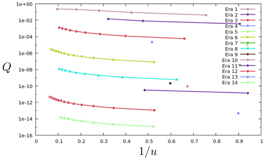
Figure 9: In this figure the graphical results of a sample of the numerical simulation are portrayed. The polymer BKL map (124) has been evolved starting from the initial value $(u=10,Q=0.24)$. Every point is the result of a single iteration of the BKL map. The role played by the Polymer BKL map (124) is just to take a single point and map it to the next one. A total of 14 Kasner eras are shown, each with a different color. The fact that, starting from the upmost point, the map on $Q$ is almost always decreasing is very evident from the downwards-going ladder-like shape of the eras.

From the results of the numerical simulations the following conclusions can be drawn:

• The polymer BKL map (124) is “well behaved” for any tested initial condition $u\in[1,\infty)$ and $Q\in[0,0.96]$: the dominion of definition for $u$ and $Q$ are preserved.

• The line $Q=0$ is an attractor for the Polymer BKL map: for any tested initial condition, the Polymer BKL map eventually evolved until becoming arbitrarily close to the standard BKL map.

• The Polymer BKL map on $Q$ is almost everywhere decreasing. It can happen that, especially for initial values $Q\approx 1$, for very few iterations the map on $Q$ is increasing, but the overall behavior is almost always decreasing. The probability to have an increasing behavior of $Q$ gets smaller at every iteration. In the limit of infinitely many iterations this probability goes to zero.

• Since the Polymer BKL map (124) tends asymptotically to the standard BKL map (39), we expect that the notion of chaos for the standard BKL map, given for example in Barrow:1982 , can be applied, with little or no modifications, to the Polymer case, too (although this has not been proven rigorously).

8 Physical considerations

In this section we address two basic questions concerning the physical link between Polymer and Loop quantization methods and what happens when all the Minisuperspace variables are discrete, respectively.

First of all, we observe that Polymer Quantum Mechanics is an independent approach from Loop Quantum Gravity. Using the Polymer procedure is equivalent to implement a sort of discretization of the considered configurational variables. Each variable is treated separately, by introducing a suitable graph (de facto a one-dimensional lattice structure): the group of spatial translations on this graph is a $U(1)$ type, therefore the natural group of symmetry underlying such quantization method is $U(1)$ too, differently from Loop Quantum Gravity, where the basic group of symmetry is $SU(2)$.

It is important to stress that Polymer Quantum Mechanics is not unitary connected to the standard Quantum Mechanics, since the Stone - Von Neumann theorem is broken in the discretized representation. Even more subtle is that Polymer quantization procedures applied to different configurational representations of the same system are, in general, not unitary related. This is clear in the zero order WKB limit of the Polymer quantum dynamics, where the formulations in two sets of variables, which are canonically related in the standard Hamiltonian representation, are no longer canonically connected in the Polymer scenario, mainly due to the non-trivial implications of the prescription for the momentum operator.

When the Loop Quantum Gravity Cianfrani:2014 ; Thiemann:2007loop is applied to the Primordial Universe, due to the homogeneity constraint underlying the Minisuperspace structure, it loses the morphology of a $SU(2)$ gauge theory (this point is widely discussed in Cianfrani:2010ji ; Cianfrani:2011wg ) and the construction of a kinematical Hilbert space, as well as of the geometrical operators, is performed by an effective, although rigorous, procedure. A discrete scale is introduced in the Holonomy definition, taken on a square of given size and then the curvature term, associated to the Ashtekar-Barbero-Immirzi connection, (the so-called Euclidean term of the scalar constraint) is evaluated on such a square path. It seems that just in this step the Loop Quantum Cosmology acquires the features of a polymer graph, associated to an underlying $U(1)$ symmetry. The real correspondence between the two approaches emerges in the semi-classical dynamics of the Loop procedure Ashtekar:2002 , which is isomorphic to the zero order WKB limit of the Polymer quantum approach. In this sense, the Loop Quantum Cosmology studies legitimate the implementation of the Polymer formalism to the cosmological Minisuperspace.

However, if on one hand, the Polymer quantum cosmology predictions are, to some extent, contained in the Loop Cosmology, on the other hand, the former is more general because it is applicable to a generic configurational representation, while the latter refers specifically to the Ashtekar-Berbero-Immirzi connection variable.

Thus, the subtle question arises about which is the proper set of variables in order that the implementation of the Polymer procedure mimics the Loop treatment, as well as which is the physical meaning of different Polymer dynamical behaviours in different sets of variables. In Mantero:2018cor it is argued, for the isotropic Universe quantization, that the searched correspondence holds only if the cubed scale factor is adopted as Polymer variable: in fact this choice leads to a critical density of the Universe which is independent of the scale factor and a direct link between the Polymer discretization step and the Immirzi parameter is found. This result assumes that the Polymer parameter is maintained independent of the scale factor, otherwise the correspondence above seems always possible. In this respect, different choices of the configuration variables when Polymer quantizing a cosmological system could be mapped into each other by suitable re-definition of the discretization step as a function of the variables themselves. Here we apply the Polymer procedure to the Misner isotropic variable and not to the cubed scale factor, so that different issues with respect to Loop Quantum Gravity can naturally emerge. The merit of the present choice is that we discretize the volume of the Universe, without preventing its vanishing behavior. This can be regarded as an effective procedure to include the zero-volume eigenvalue in the system dynamics, like it can happen in Loop Quantum Gravity, but it is no longer evident in its cosmological implementation.

Thus, no real contradiction exists between the present study and the Big-Bounce prediction of the Loop formulation, since they are expectedly two independent physical representations of the same quantum system. As discussed on the semi-classical level in Antonini:2018gdd , when using the cubed scale factor as isotropic dynamics, the Mixmaster model becomes non-singular and chaos free, just as predicted in the Loop Quantum Cosmology analysis presented in Bojowald:2004 . However, in such a representation, the vanishing behavior of the Universe volume is somewhat prevented a priori, by means of the Polymer discretization procedure.

Finally, we observe that, while in the present study, the Polymer dynamics of the isotropic variable $\alpha$ preserves (if not even enforces) the Mixmaster chaos, in Montani:2013 the Polymer analysis for the anisotropic variables $\beta_{\pm}$ is associated to the chaos disappearance. This feature is not surprising since the two approaches have a different physical meaning: the discretization of $\alpha$ has to do with geometrical properties of the space-time (it can be thought as an embedding variable), while the implementation of the Polymer method to $\beta_{\pm}$ really affects the gravitational degrees of freedom of the considered cosmological model.

Nonetheless, it becomes now interesting to understand what happens to the Mixmaster chaotic features when the two sets of variables ($\alpha$ and $\beta_{\pm}$) are simultaneously Polymer quantized. In the following subsection, we provide an answer to such an intriguing question, at least on the base of the semi-classical dynamics.

8.1 The polymer approach applied to the whole Minisuperspace

According to the polymer prescription (55), the super - Hamiltonian constraint is now:

$$\mathcal{H}=\frac{B\kappa}{3(8\pi)^{2}}e^{-3\alpha}\left(-\frac{1}{\mu_{\alpha}^{2}}\sin^{2}(\mu_{\alpha}p_{\alpha})+\frac{1}{\mu^{2}}\sin^{2}(\mu p_{+})+\right.\\ \left.+\frac{1}{\mu^{2}}\sin^{2}(\mu p_{-})+\frac{3(4\pi)^{4}}{\kappa^{2}}e^{4\alpha}V_{B}(\beta_{\pm})\right)=0$$ (126)

where $\mu_{\alpha}$ is the polymer parameter associated to $\alpha$ and $\mu$ the one associated to $\beta_{\pm}$. The dynamics of the system can be derived through the Hamilton’s equations (44). As usual, we start considering the simple Bianchi I case $V_{B}=0$. Following the procedure of Sec. 6.1, we find that the Universe is still singular. In fact, the solution to Hamilton’s equations in the (88) time gauge (with $\mu_{\alpha}$ instead of $\mu$) is:

$$\alpha(t) =\frac{1}{3}\ln(t)$$ (127a)

$$\beta_{\pm}(t) =-\frac{1}{3}\frac{\sin(2\mu p_{\pm})}{\sin(2\mu_{\alpha}p_{\alpha})}\ln(t)$$ (127b)

from which it follows that $\alpha(t)\rightarrow-\infty$ as $t\to 0$. Moreover, the sum of the squared Kasner indices, calculated by making a reverse canonical transformation from Misner to ordinary variables, reads as:

$$p_{l}^{2}+p_{m}^{2}+p_{n}^{2}=\frac{1}{3}\left(1+2\frac{\sin^{2}(2\mu p_{+})+\sin^{2}(2\mu p_{-})}{\sin^{2}(2\mu_{\alpha}p_{\alpha})}\right)$$ (128)

from which is possible to derive the anisotropy velocity, according to Eq. (92)). The anisotropy velocity can be also calculated through the ADM reduction method, as in Sec. 5.1. The new reduced Hamiltonian is:

$$H_{poly}=\frac{1}{\mu_{\alpha}}\arcsin\left(\sqrt{\frac{\mu_{\alpha}^{2}}{\mu^{2}}(\sin^{2}(\mu p_{+})+\sin^{2}(\mu p_{-}))}\right)$$ (129)

and from the Hamilton’s equation for $\beta_{\pm}$:

$$\beta^{\prime}_{\pm}\equiv\frac{d\beta_{\pm}}{d\alpha}=\frac{\sin(\mu p_{\pm})\cos(\mu p_{\pm})}{\sqrt{\left[1-\frac{\mu_{\alpha}^{2}}{\mu^{2}}(\sin^{2}(\mu p_{+})+\sin^{2}(\mu p_{-}))\right](\sin^{2}(\mu p_{+})+\sin^{2}(\mu p_{-}))}}$$ (130)

we derive:

$$\beta^{\prime}\equiv\sqrt{\beta^{\prime 2}_{+}+\beta^{\prime^{\prime}}_{-}}=\\ =\sqrt{\frac{\sin^{2}(\mu p_{+})\cos^{2}(\mu p_{+})+\sin^{2}(\mu p_{-})\cos^{2}(\mu p_{-})}{\left[1-\frac{\mu_{\alpha}^{2}}{\mu^{2}}(\sin^{2}(\mu p_{+})+\sin^{2}(\mu p_{-}))\right](\sin^{2}(\mu p_{+})+\sin^{2}(\mu p_{-}))}}$$ (131)

that turns out to be greater than one when $\mu_{\alpha}\geq\mu$ (see Fig. 10).

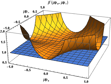
Figure 10: Anisotropy velocity (131) (when $\mu_{\alpha}=\mu$) as a function of $(\mu p_{+},\mu p_{-})$ compared with the standard anisotropy velocity $\beta^{\prime}=1$.

Finally, it should be noted that since in the general $V_{B}\neq 0$ case the wall velocity $\beta^{\prime}_{wall}$ is not influenced by the introduction of the polymer quantization, from Eq. (131) we find that the maximum incident angle for having a bounce against a given potential wall $\left(\theta_{max}=\arccos\left(\frac{\beta^{\prime}_{wall}}{\beta^{\prime}}\right)\right)$ is, also in this case, always greater than $\pi/3$ when $\mu_{\alpha}\geq\mu$. We can then conclude that also when the polymer approach is applied to all the three configuration variables simultaneously, the Universe can be singular and chaotic just such as the one analyzed above.

9 Conclusions

In the present study, we analyzed the Mixmaster model in the framework of the semiclassical Polymer Quantum Mechanics, implemented on the isotropic Misner variable, according to the idea that the cut-off physics mainly concerns the Universe volume.

We developed a semiclassical and quantum dynamics, in order to properly characterize the structure of the singularity, still present in the model. The presence of the singularity is essentially due to the character of the isotropic variable conjugate momentum as a constant of motion.

On the semiclassical level we studied the system evolution both in the Hamiltonian and field equations representation, generalizing the two original analyses in Misner:1969 and Belinskii:1970 , respectively. The two approaches are converging and complementary, describing the initial singularity of the Mixmaster model as reached by a chaotic dynamics, that is, in principle, more complex than the General Relativity one, but actually coincides with it in the asymptotic limit.

This issue is a notable feature, since in Loop Quantum Cosmology is expected that the Bianchi IX model is chaos-free Bojowald:2004 ; Bojowald:2004ra and it is well known Ashtekar:2001xp that the Polymer semiclassical dynamics closely resembles the average feature of a Loop treatment in the Minisuperspace. However, we stress that, while the existence of the singularity in Polymer Quantum Mechanics appears to be a feature depending on the nature of the adopted configuration variables, nonetheless the properties of the Poincaré map of the model is expected to be a solid physical issue, independent on the particular representation adopted for the system.

The canonical quantization of the Mixmaster Universe that we performed in the full Polymer quantum approach, i.e. writing down a Wheeler-DeWitt equation in the momentum representation, accordingly to the so-called Continuum Limit discussed in Corichi:2007pr , is completely consistent with the semiclassical results. In fact, the Misner demonstration, for the standard canonical approach, that states with high occupation numbers can survive to the initial singularity, remains still valid in the Polymer formulation, here presented. This issue confirms that the cut-off we introduced in the configuration space on the isotropic Misner variable does not affect the cosmological character of the Mixmaster model.

This result appears rather different from the analysis in Montani:2013 , where the polymer approach has been addressed for the anisotropic Misner variables (the real degrees of freedom of the cosmological gravitational field) with the emergence of a non-chaotic cosmology. Such a discrepancy suggests that the Polymer regularization of the asymptotic evolution to the singularity produces more profound modifications when it touches physical properties than geometrical features. Actually, the isotropic Misner variable can be suitably interpreted as a good time variable for the system (an embedding variable in the language of Isham:1985 ; Isham:1985bis ), while the Universe anisotropies provide a precise physical information on the considered cosmological model.

Despite this consideration about the gauge-like nature of the Misner isotropic variable, which shed light on the physics of our dynamical results, nonetheless we regard as important to perform further investigations on the nature of the singularity when other variables are considered to characterize the Universe volume, since we expect that, for some specific choice the regularization of the Big-Bang to the Big-Bounce must take place (see for instance Antonini:2018gdd ). However, even on the basis of the present analysis, we suggest that the features of the Poincaré map of the Bianchi IX model and then of the generic cosmological singularity (locally mimicked by the same Bianchi IX-like time evolution) is a very general and robust property of the primordial Universe, not necessarily connected with the existence of a cut-off physics on the singularity.

- (1) L.D. Landau, E.M. Lifshitz, The Classical Theory of Fields, Fourth Edition: Volume 2 (Course of Theoretical Physics Series), 4th edn. (Butterworth-Heinemann, 1980). URL http://www.worldcat.org/isbn/0750627689
- (2) C. Misner, K. Thorne, J. Wheeler, Gravitation (W.H.Freeman, 1973)
- (3) L. Grishchuk, A. Doroshkevich, V. Iudin, Zhurnal Eksperimental’noi i Teoreticheskoi Fiziki 69, 1857 (1975)
- (4) A. Doroshkevich, V. Lukash, I. Novikov, Sov. Phys.–JETP 37, 739 (1973)
- (5) A.A. Kirillov, G. Montani, Phys. Rev. D66, 064010 (2002). DOI 10.1103/PhysRevD.66.064010
- (6) G. Montani, M.V. Battisti, R. Benini, G. Imponente, International Journal of Modern Physics A 23(16n17), 2353 (2008). DOI 10.1142/S0217751X08040275. URL https://doi.org/10.1142/S0217751X08040275
- (7) V. Belinskii, I. Khalatnikov, E. Lifshitz, Advances in Physics 19(80), 525 (1970). DOI 10.1080/00018737000101171. URL https://doi.org/10.1080/00018737000101171
- (8) C.W. Misner, Phys. Rev. 186, 1319 (1969). DOI 10.1103/PhysRev.186.1319. URL https://link.aps.org/doi/10.1103/PhysRev.186.1319
- (9) C.W. Misner, Phys. Rev. Lett. 22, 1071 (1969). DOI 10.1103/PhysRevLett.22.1071. URL https://link.aps.org/doi/10.1103/PhysRevLett.22.1071
- (10) V. Belinskii, I. Khalatnikov, E. Lifshitz, Advances in Physics 31(6), 639 (1982). DOI 10.1080/00018738200101428. URL http://dx.doi.org/10.1080/00018738200101428
- (11) A. Kirillov, JETP 76(3), 355 (1993)
- (12) G. Montani, Classical and Quantum Gravity 12(10), 2505 (1995). URL http://stacks.iop.org/0264-9381/12/i=10/a=010
- (13) G. Montani, M. Battisti, R. Benini, Primordial Cosmology (World Scientific, 2011). URL http://books.google.it/books?id=XRLv7P-V-ocC
- (14) J.M. Heinzle, C. Uggla, Class. Quant. Grav. 26, 075016 (2009). DOI 10.1088/0264-9381/26/7/075016
- (15) J.D. Barrow, F.J. Tipler, Physics Reports 56(7), 371 (1979). DOI https://doi.org/10.1016/0370-1573(79)90097-8. URL http://www.sciencedirect.com/science/article/pii/0370157379900978
- (16) B.S. DeWitt, Phys. Rev. 160, 1113 (1967). DOI 10.1103/PhysRev.160.1113. URL https://link.aps.org/doi/10.1103/PhysRev.160.1113
- (17) R. Graham, H. Luckock, Phys. Rev. D 49, 2786 (1994). DOI 10.1103/PhysRevD.49.2786. URL https://link.aps.org/doi/10.1103/PhysRevD.49.2786
- (18) F. Cianfrani, O. Lecian, M. Lulli, G. Montani, Canonical Quantum Gravity: Fundamentals and Recent Developments (World Scientific, 2014). URL https://books.google.co.jp/books?id=OuF1ngEACAAJ
- (19) C. Rovelli, L. Smolin, Nuclear Physics B 442(3), 593 (1995). DOI https://doi.org/10.1016/0550-3213(95)00150-Q. URL http://www.sciencedirect.com/science/article/pii/055032139500150Q
- (20) A. Ashtekar, T. Pawlowski, P. Singh, Physical review letters 96(14), 141301 (2006)
- (21) A. Ashtekar, T. Pawlowski, P. Singh, Physical Review D 73(12), 124038 (2006)
- (22) G. Montani, A. Marchi, R. Moriconi, Phys. Lett. B777, 191 (2018). DOI 10.1016/j.physletb.2017.12.016
- (23) J.D. Barrow, C. Ganguly, Phys. Rev. D95(8), 083515 (2017). DOI 10.1103/PhysRevD.95.083515
- (24) A. Ashtekar, A. Henderson, D. Sloan, Class. Quant. Grav. 26, 052001 (2009). DOI 10.1088/0264-9381/26/5/052001
- (25) A. Ashtekar, A. Henderson, D. Sloan, Phys. Rev. D83, 084024 (2011). DOI 10.1103/PhysRevD.83.084024
- (26) M. Bojowald, G. Date, G.M. Hossain, Class. Quant. Grav. 21, 3541 (2004). DOI 10.1088/0264-9381/21/14/015
- (27) M. Bojowald, G. Date, Phys. Rev. Lett. 92, 071302 (2004). DOI 10.1103/PhysRevLett.92.071302
- (28) A. Ashtekar, J. Lewandowski, Class. Quant. Grav. 18, L117 (2001). DOI 10.1088/0264-9381/18/18/102
- (29) A. Corichi, T. Vukasinac, J.A. Zapata, Phys. Rev. D76, 044016 (2007). DOI 10.1103/PhysRevD.76.044016
- (30) O.M. Lecian, G. Montani, R. Moriconi, Phys. Rev. D88(10), 103511 (2013). DOI 10.1103/PhysRevD.88.103511
- (31) R. Moriconi, G. Montani, Phys. Rev. D95(12), 123533 (2017). DOI 10.1103/PhysRevD.95.123533
- (32) M.V. Battisti, O.M. Lecian, G. Montani, Phys. Rev. D78, 103514 (2008). DOI 10.1103/PhysRevD.78.103514
- (33) G.M. Hossain, V. Husain, S.S. Seahra, Physical Review D 81(2), 024005 (2010)
- (34) G. De Risi, R. Maartens, P. Singh, Physical Review D 76(10), 103531 (2007)
- (35) S.M. Hassan, V. Husain, Classical and Quantum Gravity 34(8), 084003 (2017)
- (36) S.S. Seahra, I.A. Brown, G.M. Hossain, V. Husain, Journal of Cosmology and Astroparticle Physics 2012(10), 041 (2012)
- (37) J. Sakurai, J. Napolitano, Modern Quantum Mechanics (Addison-Wesley, 2011). URL https://books.google.it/books?id=N4I-AQAACAAJ
- (38) C. Rovelli, S. Speziale, Phys. Rev. D67, 064019 (2003). DOI 10.1103/PhysRevD.67.064019
- (39) A.A. Kirillov, G. Montani, Phys. Rev. D 56, 6225 (1997). DOI 10.1103/PhysRevD.56.6225. URL https://link.aps.org/doi/10.1103/PhysRevD.56.6225
- (40) G. Imponente, G. Montani, Phys. Rev. D63, 103501 (2001). DOI 10.1103/PhysRevD.63.103501
- (41) H. Salecker, E.P. Wigner, Phys. Rev. 109, 571 (1958). DOI 10.1103/PhysRev.109.571. URL https://link.aps.org/doi/10.1103/PhysRev.109.571
- (42) G. Amelino-Camelia, Phys. Lett. B477, 436 (2000). DOI 10.1016/S0370-2693(00)00231-8
- (43) S. Hossenfelder, Living Rev. Rel. 16, 2 (2013). DOI 10.12942/lrr-2013-2
- (44) A. Ashtekar, P. Singh, Class. Quant. Grav. 28, 213001 (2011). DOI 10.1088/0264-9381/28/21/213001
- (45) J.E. Lidsey, D. Wands, E.J. Copeland, Phys. Rept. 337, 343 (2000). DOI 10.1016/S0370-1573(00)00064-8
- (46) A. Ashtekar, S. Fairhurst, J.L. Willis, Class. Quant. Grav. 20, 1031 (2003). DOI 10.1088/0264-9381/20/6/302
- (47) A. Ashtekar, J. Lewandowski, H. Sahlmann, Classical and Quantum Gravity 20(1), L11 (2003). URL http://stacks.iop.org/0264-9381/20/i=1/a=103
- (48) M. Varadarajan, Phys. Rev. D61, 104001 (2000). DOI 10.1103/PhysRevD.61.104001
- (49) A. Corichi, T. Vukasinac, J.A. Zapata, Class. Quant. Grav. 24, 1495 (2007). DOI 10.1088/0264-9381/24/6/008
- (50) E. Binz, S. Pods, The Geometry of Heisenberg Groups: With Applications in Signal Theory, Optics, Quantization, and Field Quantization. Mathematical surveys and monographs (American Mathematical Society, 2008). URL https://books.google.co.jp/books?id=yIP0BwAAQBAJ
- (51) W. Arveson, An Invitation to C*-Algebras. Graduate Texts in Mathematics (Springer New York, 1998). URL https://books.google.co.jp/books?id=zRep59fhoGkC
- (52) W. Rudin, Fourier Analysis on Groups (Wiley, 2011). URL https://books.google.it/books?id=k3RNtFSBH8gC
- (53) J. Wainwright, A. Krasiński, General Relativity and Gravitation 40(4), 865 (2008). DOI 10.1007/s10714-007-0574-4. URL https://doi.org/10.1007/s10714-007-0574-4
- (54) W. contributors. Bkl singularity — wikipedia, the free encyclopedia (2017). URL {https://en.wikipedia.org/w/index.php?title=BKL_singularity&oldid=799333893}. [Online; accessed 26-December-2017]
- (55) J.D. Barrow, Phys. Rev. Lett. 46, 963 (1981). DOI 10.1103/PhysRevLett.46.963. URL https://link.aps.org/doi/10.1103/PhysRevLett.46.963
- (56) J.D. Barrow, Physics Reports 85(1), 1 (1982). DOI https://doi.org/10.1016/0370-1573(82)90171-5. URL http://www.sciencedirect.com/science/article/pii/0370157382901715
- (57) I.M. Khalatnikov, E.M. Lifshitz, K.M. Khanin, L.N. Shchur, Ya.G. Sinai, Fundam. Theor. Phys. 9, 343 (1984). DOI 10.1007/978-94-009-6469-3_18
- (58) E.M. Lifshitz, I.M. Lifshitz, I.M. Khalatnikov, Soviet Journal of Experimental and Theoretical Physics 32, 173 (1971)
- (59) M. Szydlowski, A. Krawiec, Phys. Rev., D 47(12), 5323 (1993)
- (60) R. Arnowitt, S. Deser, C.W. Misner, Phys. Rev. 117, 1595 (1960). DOI 10.1103/PhysRev.117.1595. URL https://link.aps.org/doi/10.1103/PhysRev.117.1595
- (61) A. Ashtekar, T. Pawlowski, P. Singh, K. Vandersloot, Phys. Rev. D75, 024035 (2007). DOI 10.1103/PhysRevD.75.024035
- (62) A. Ashtekar, E. Wilson-Ewing, Phys. Rev. D79, 083535 (2009). DOI 10.1103/PhysRevD.79.083535
- (63) M.V. Battisti, Submitted to: Phys. Rev. D (2008)
- (64) M. Battisti, G. Montani, Phys. Lett. B 681, 179 (2009). DOI 10.1016/j.physletb.2009.10.003
- (65) G. Montani, Int. J. Mod. Phys. D13, 1029 (2004). DOI 10.1142/S0218271804004967
- (66) Y. Elskens, M. Henneaux, Nuclear Physics B 290(Supplement C), 111 (1987). DOI https://doi.org/10.1016/0550-3213(87)90180-5. URL http://www.sciencedirect.com/science/article/pii/0550321387901805
- (67) M. Tenenbaum, H. Pollard, Ordinary Differential Equations. Dover Books on Mathematics Series (Dover Publications, Incorporated, 2012). URL https://books.google.it/books?id=29utVed7QMIC
- (68) A.R. Moser, R.A. Matzner, M.P. Ryan, Annals of Physics 79(2), 558 (1973). DOI https://doi.org/10.1016/0003-4916(73)90097-3. URL http://www.sciencedirect.com/science/article/pii/0003491673900973
- (69) B.K. Berger, Living Reviews in Relativity 5(1), 1 (2002). DOI 10.12942/lrr-2002-1. URL https://doi.org/10.12942/lrr-2002-1
- (70) T. Thiemann, in Approaches to Fundamental Physics (Springer, 2007), pp. 185–263
- (71) F. Cianfrani, G. Montani, Phys. Rev. D82, 021501 (2010). DOI 10.1103/PhysRevD.82.021501
- (72) F. Cianfrani, G. Montani, Phys. Rev. D85, 024027 (2012). DOI 10.1103/PhysRevD.85.024027
- (73) C. Mantero, G. Montani, F. Bombacigno, (2018)
- (74) S. Antonini, G. Montani, (2018)
- (75) C.J. Isham, K.V. Kuchar, Annals of Physics 164(2), 288 (1985)
- (76) C.J. Isham, K.V. Kuchar, Annals of Physics 164(2), 316 (1985)