On the sensitivity to model parameters in a filter stabilization technique for advection dominated advection-diffusion-reaction problems

Abstract

We consider a filter stabilization technique with a deconvolution-based indicator function for the simulation of advection dominated advection-diffusion-reaction (ADR) problems with under-refined meshes. The proposed technique has been previously applied to the incompressible Navier-Stokes equations and has been successfully validated against experimental data. However, it was found that some key parameters in this approach have a strong impact on the solution. To better understand the role of these parameters, we consider ADR problems, which are simpler than incompressible flow problems. For the implementation of the filter stabilization technique to ADR problems we adopt a three-step algorithm that requires (i) the solution of the given problem on an under-refined mesh, (ii) the application of a filter to the computed solution, and (iii) a relaxation step. We compare our deconvolution-based approach to classical stabilization methods and test its sensitivity to model parameters on a 2D benchmark problem.

1 Introduction

We adapt to time-dependent advection-diffusion-reaction (ADR) problems a filter stabilization technique proposed in Ervin_et_al2012 for evolution equations and mostly developed for the Navier-Stokes equations Ervin_et_al2012 ; layton_CMAME ; abigail_CMAME . This technique applied to the Navier-Stokes equations has been extensively tested on both academic problems Ervin_et_al2012 ; layton_CMAME ; abigail_CMAME and realistic applications BQV ; Xu2018 . It was found in BQV that key parameters in this approach have a strong impact on the solution. In order to understand the role of these key parameters, we apply the filter stabilization technique in the simplified context of ADR problems.

It is well known that the Galerkin method for advection dominated ADR problems can lead to unstable solutions with spurious oscillations B-quarteroniv2 ; C-hughes2 ; brooksh ; hughesf4 ; douglasw1 ; hughes1 ; codina2 . The proposed stabilization technique cures these oscillations by using an indicator function to tune the amount and location of artificial viscosity. The main advantage of this technique is that it can be easily implemented in legacy solvers.

2 Problem definition

We consider a time-dependent advection-diffusion-reaction problem defined on a bounded domain $\Omega\in\mathbb{R}^{d}$, with $d=2,3$, over a time interval of interest $(0,T]$:

$$\partial_{t}u-\mu\Delta u+\nabla\cdot({\bf b}u)+\sigma u=f\quad\text{in}~{}\Omega\times(0,T],$$ (1)

endowed with boundary conditions:

$$u=u_{D}\quad\quad\quad\text{on}~{}\partial\Omega_{D}\times(0,T],$$ (2)

$$\mu\nabla u\cdot{\bf n}=g\quad\text{on}~{}\partial\Omega_{N}\times(0,T],$$ (3)

and initial condition $u=u_{0}$ in $\Omega\times\{0\}$. Here $\overline{\partial\Omega_{D}}\cup\overline{\partial\Omega_{N}}=\overline{\partial\Omega}$ and $\partial\Omega_{D}\cap\partial\Omega_{N}=\emptyset$ and $u_{D}$, $g$, and $u_{0}$ are given. In (1)-(3), $\mu$ is a diffusion coefficient, ${\bf b}$ is an advection field, $\sigma$ is a reaction coefficient, and $f$ is the forcing term. For the sake of simplicity, we consider $\mu$, ${\bf b}$, and $\sigma$ constant.

Let $L$ be a characteristic macroscopic length for problem (1)-(3). To characterize the solution of problem (1)-(3), we introduce the Péclet number: $\displaystyle{\mathbb{P}\text{e}=||{\bf b}||_{\infty}L/(2\mu)}$. We will assume that the problem is convection dominated, i.e. $||{\bf b}||_{\infty}\gg\mu$, which implies large Péclet numbers. Notice that the role of the $\mathbb{P}\text{e}$ for advection-diffusion-reaction problems is similar to the role played by the Reynolds number for the Navier-Stokes equations.

In order to write the variational formulation of problem (1)-(3), we define the following spaces:

$$V =\left\{v:\Omega\rightarrow\hbox{\doble R},~{}v\in H^{1}({\Omega}),~{}v=u_{D}~{}\text{on}~{}\partial\Omega_{D}\right\},$$

$$V_{0} =\left\{v:\Omega\rightarrow\hbox{\doble R},~{}v\in H^{1}({\Omega}),~{}v=0~{}\text{on}~{}\partial\Omega_{D}\right\}.$$

and bilinear form

$$b(u,w)=(\mu\nabla u,\nabla w)_{\Omega}+(\nabla\cdot({\bf b}u),w)_{\Omega}+(\sigma u,w)_{\Omega},\quad\forall u\in V,~{}\forall w\in V_{0}.$$ (4)

The variational form of problem (1)-(3) reads: Find $u\in V$ such that

$$(\partial_{t}u,w)_{\Omega}+b(u,w)=(f,w)_{\Omega}+(g,w)_{\partial\Omega_{N}},\quad\forall w\in V_{0}.$$ (5)

The conditions for existence and unicity of the solution of problem (5) can be found, e.g., in (B-quarteroniv2, , Chapter 12).

For the time discretization of problem (5), we consider the backward Euler scheme for simplicity. Let $\Delta t\in\mathbb{R}$, $t^{n}=n\Delta t$, with $n=0,...,N_{T}$ and $T=N_{T}\Delta t$. We denote by $y^{n}$ the approximation of a generic quantity $y$ at the time $t^{n}$. Problem (5) discretized in time reads: given $u^{0}=u_{0}$, for $n\geq 0$ find $u^{n+1}\in V$ such that

$$\frac{1}{\Delta t}(u^{n+1},w)_{\Omega}+b(u^{n+1},w)=\frac{1}{\Delta t}(u^{n},w)_{\Omega}+(f^{n+1},w)_{\Omega}+(g^{n+1},w)_{\partial\Omega_{N}},$$ (6)

$\forall w\in V_{0}$. We remark that time discretization approximates problem (5) by a sequence of quasi-static problems (6). In fact, we can think of eq. (6) as the variational formulation of problem:

$$L_{t}u^{n+1}={f}_{t}^{n+1},$$ (7)

where

$$L_{t}u^{n+1}=-\mu\Delta u^{n+1}+\nabla\cdot({\bf b}u^{n+1})+\left(\sigma+\frac{1}{\Delta t}\right)u^{n+1},~{}{f}_{t}^{n+1}=\frac{u^{n}}{\Delta t}+f^{n+1}.$$

With regard to space discretization, we use the Finite Element method. Let $\mathcal{T}_{h}=\{K\}$ be a generic, regular Finite Element triangulation of the domain $\Omega$ composed by a set of finite elements, indicated by $K$. As usual, $h$ refers to the largest diameter of the elements of $\mathcal{T}_{h}$. Let $V_{h}$ and $V_{0,h}$ be the finite element spaces approximating $V$ and $V_{0}$, respectively. The fully discrete problem reads: given $u^{0}_{h}$, for $n\geq 0$ find $u^{n+1}_{h}\in V_{h}$ such that

$$\frac{1}{\Delta t}(u^{n+1}_{h},w)_{\Omega}+b(u^{n+1}_{h},w)=\frac{1}{\Delta t}(u^{n}_{h},w)_{\Omega}+(f^{n+1}_{h},w)_{\Omega}+(g^{n+1}_{h},w)_{\partial\Omega_{N}},$$ (8)

$\forall w\in V_{0,h}$, where $u^{0}_{h}$, $f^{n+1}_{h}$, and $g^{n+1}_{h}$ are appropriate finite element approximations of $u_{0}$, $f^{n+1}$, and $g^{n+1}$, respectively. It is known that the solution of problem (8) converges optimally to the solution of problem (5). However, the Finite Element method can perform poorly if the coerciveness constant of the bilinear form (4) is small in comparison with its continuity constant. In particular, the error estimate can have a very large multiplicative constant if $\mu$ is small with respect to $||{\bf b}||_{\infty}$, i.e. when $\mathbb{P}\text{e}$ is large. In those cases, the finite element solution $u_{h}$ can be globally polluted with strong spurious oscillations. To characterize the solution of problem (8), we introduce the local counterpart of the Péclet number: $\displaystyle{\mathbb{P}\text{e}_{h}=||{\bf b}||_{\infty}h/(2\mu)}$.

Several stabilization techniques have been proposed to eliminate, or at least reduce, the numerical oscillations produced by the standard Galerkin method in case of large $\mathbb{P}\text{e}$. In the next section, we will go over a short review of these stabilization techniques before introducing our filter stabilization method in Sec. 3.

2.1 Overview of stabilization techniques

We will restrict our attention to stabilization techniques that consists of adding a stabilization term $b_{s}(u^{n+1}_{h},w)$ to the left-hand side of time-discrete problem (6). In the following, we will use $\tau$ to denote a stabilization parameter that can depend on the element size $h$ and the equation coefficients. Parameter $\tau$ takes different values for the different stabilization schemes. We will use the broken inner product $(\cdot,\cdot)_{K}=\sum_{K}(\cdot,\cdot)$, where $\sum_{K}$ denotes summation over all the finite elements.

Perhaps the easiest way to stabilize problem (6) is by introducing artificial viscosity either in the whole domain, leading to $b_{s}(u^{n+1}_{h},w)=(\tau\nabla u_{h}^{n+1},\nabla w)_{K}$, or streamwise, leading to $b_{s}(u^{n+1}_{h},w)=(\tau{\bf b}\cdot\nabla u_{h}^{n+1},{\bf b}\cdot\nabla w)_{K}$. See, e.g., C-hughes2 ; B-quarteroniv2 . In this way, the effective $\mathbb{P}\text{e}_{h}$ becomes smaller. The artificial viscosity $\tau$ in these schemes is proportional to $h$. The drawbacks of these schemes are that they are first order accurate only and not strongly consistent. An improvement over the artificial viscosity schemes is given by the strongly consistent stabilization methods. In fact, strong consistency allows the stabilized method to maintain the optimal accuracy.

Let us introduce the residual for problem (7) and the skew-symmetric part of operator $L_{t}$:

$$R(u_{h}^{n+1})={f}_{t}^{n+1}-L_{t}u_{h}^{n+1},\quad L_{SS}v=\frac{1}{2}\nabla\cdot({\bf b}v)+\frac{1}{2}{\bf b}\cdot\nabla v.$$

One of the most popular strongly consistent stabilized finite element methods is the Streamline Upwind Petrov-Galerkin (SUPG) method brooksh , for which $b_{s}(u^{n+1}_{h},w)=-(\tau R(u_{h}^{n+1}),L_{SS}w)_{K}$. The Galerkin Least Squares (GLS) method hughesf4 is a generalization of the SUPG method: $b_{s}(u^{n+1}_{h},w)=-(\tau R(u_{h}^{n+1}),L_{t}w)_{K}$. The Douglas-Wang method douglasw1 replaces $L_{t}w$ in the GLS method with $-L_{t}^{*}w$, where $L_{t}^{*}$ is the adjoint of operator $L_{t}$. Thus, we have: $b_{s}(u^{n+1}_{h},w)=(\tau R(u_{h}^{n+1}),L_{t}^{*}w)_{K}$. For the SUPG, GLS, and Douglas-Wang methods, $\tau=\delta h_{K}/|{\bf b}|$ for $\delta>0$. Finally, we mention a method based on the Variational Multilscale approach hughes1 called algebraic subgrid scale (ASGS), for which $b_{s}(u^{n+1}_{h},w)=(\tau R(u_{h}^{n+1}),L_{t}^{*}w)_{K}$. The difference between the Douglas-Wang and ASGS method consists in the choice for parameter $\tau$. One possibility for $\tau$ in the ASGS method is $\tau=[4\mu/h_{K}^{2}+2|{\bf b}|/h_{K}+\sigma]^{-1}$ (see codina2 ).

We report in Table 1 a summary of the methods in this overview. All of the strongly consistent stabilization techniques come with stability estimates that improve the one that can be obtained for the Galerkin method. See brooksh ; hughesf4 ; douglasw1 ; B-quarteroniv2 ; hughes1 ; codina2 .

Table 1: Stabilization term $b_{s}(u^{n+1}_{h},w)$ for some stabilization methods.

	Stabilization method	$b_{s}(u^{n+1}_{h},w)$
Not strongly consistent	Artificial viscosity	$(\tau\nabla u_{h}^{n+1},\nabla w)_{K}$
	Streamline upwind	$(\tau{\bf b}\cdot\nabla u_{h}^{n+1},{\bf b}\cdot\nabla w)_{K}$
Strongly consistent	Streamline upwind Petrov-Galerkin	$-(\tau R(u_{h}^{n+1}),L_{SS}w)_{K}$
	Galerkin least-squares	$-(\tau R(u_{h}^{n+1}),L_{t}w)_{K}$
	Douglas-Wang	$(\tau R(u_{h}^{n+1}),L_{t}^{*}w)_{K}$
	Variational Multiscale, ASGS	$(\tau R(u_{h}^{n+1}),L_{t}^{*}w)_{K}$

3 A filter stabilization technique

We adapt to the time-dependent advection-diffusion-reaction problem defined in Sec. 2 a filter stabilization technique proposed in Ervin_et_al2012 . For the implementation of this stabilization technique we adopt an algorithm called evolve-filter-relax (EFR) that was first presented in layton_CMAME . The EFR algorithm applied to problem (7) with boundary conditions (2)-(3) reads: given $u^{n}$

1. Evolve: find the intermediate solution $v^{n+1}$ such that

   $$L_{t}v^{n+1}=f_{t}^{n+1}\quad\text{in}~{}\Omega,$$ (9)

   $$v^{n+1}=u_{D}\quad\quad\quad\text{on}~{}\partial\Omega_{D},$$ (10)

   $$\mu\nabla v^{n+1}\cdot{\bf n}=g\quad\text{on}~{}\partial\Omega_{N}.$$ (11)

2. Filter: find $\overline{v}^{n+1}$ such that

   $$\overline{v}^{n+1}-\delta^{2}\nabla\cdot(a(v^{n+1})\nabla\overline{v}^{n+1})=v^{n+1} \text{in}~{}\Omega,$$ (12)

   $$\overline{v}^{n+1}=u_{D} \text{on}~{}\partial\Omega_{D},$$ (13)

   $$\mu\nabla\overline{v}^{n+1}\cdot{\bf n}=0 \text{on}~{}\partial\Omega_{N}.$$ (14)

   Here, $\delta$ can be interpreted as the filtering radius (that is, the radius of the neighborhood were the filter extracts information) and $a(\cdot)\in(0,1]$ is a scalar function called indicator function. The indicator function has to be such that $a(v^{n+1})\simeq 1$ where $v^{n+1}$ does need to be filtered from spurious oscillations, and $a(v^{n+1})\simeq 0$ where $v^{n+1}$ does not need to be filtered.

3. Relax: set

   $$u^{n+1}=(1-\chi)v^{n+1}+\chi\overline{v}^{n+1},$$ (15)

   where $\chi\in(0,1]$ is a relaxation parameter.

The EFR algorithm has the advantage of modularity: since the problems at steps (i) and (ii) are numerically standard, they can be solved with legacy solvers without a considerable implementation effort. Algorithm (9)-(15) is sensitive to the choice of key parameters $\delta$ and $\chi$ BQV ; BQRV . A common choice for $\delta$ is $\delta=h$. However, in BQV it is suggested that taking $\delta=h$ might lead to to excessive numerical diffusion and it is proposed to set $\delta=h_{min}$, where $h_{min}$ is the length of the shortest edge in the mesh. As for $\chi$, in layton_CMAME the authors support the choice $\chi=O(\Delta t)$ because it guarantees that the numerical dissipation vanishes as $h\rightarrow 0$ regardless of $\Delta t$. In BQV the value of $\chi$ is set with a heuristic formula which depends on both physics ans discretization parameters.

Different choices of $a(\cdot)$ for the Navier-Stokes equations have been proposed and compared in layton_CMAME ; O-hunt1988 ; Vreman2004 ; Bowers2012 . Here, we focus on a class of deconvolution-based indicator functions:

$$a(u)=a_{D}(u)=\left|u-D(F(u))\right|,$$ (16)

where $F$ is a linear, invertible, self-adjoint, compact operator from a Hilbert space $V$ to itself, and $D$ is a bounded regularized approximation of $F^{-1}$. In fact, since $F$ is compact, the inverse operator $F^{-1}$ is unbounded. The composition of the two operators $F$ and $D$ can be interpreted as a low-pass filter.

A possible choice for $D$ is the Van Cittert deconvolution operator $D_{N}$, defined as

$$D_{N}=\sum_{n=0}^{N}(I-F)^{n}.$$

The evaluation of $a_{D}$ with $D=D_{N}$ (deconvolution of order $N$) requires then to apply the filter $F$ a total of $N+1$ times. Since $F^{-1}$ is not bounded, in practice $N$ is chosen to be small, as the result of a trade-off between accuracy (for a regular solution) and filtering (for a non-regular one).

We select $F$ to be the linear Helmholtz filter operator $F_{H}$ germano defined by

$$F=F_{H}\equiv\left(I-\delta^{2}\Delta\right)^{-1}.$$

It is possible to prove Dunca2005 that

$$u-D_{N}(F_{H}(u))=(-1)^{N+1}\delta^{2N+2}\Delta^{N+1}F_{H}^{N+1}u.$$ (17)

Therefore, $a_{D_{N}}(u)$ is close to zero in the regions of the domain where $u$ is smooth. Indicator function (16) with $D=D_{N}$ and $F=F_{H}$ has been proposed in abigail_CMAME for the Navier-Stokes equations. Algorithm (9)-(15) with indicator function (16) is also sensitive to the choice of $N$ BQV ; BQRV .

In order to compare our approach with the stabilization techniques reported in Sec. 2.1, let us assume that problem (1) is supplemented with homogeneous Dirichlet boundary conditions on the entire boundary, i.e. $\partial\Omega_{D}=\partial\Omega$ and $u_{D}=0$ in (2). Let us start by writing the weak form of eq. (9):

$$(L_{t}v^{n+1},w)=\left(f_{t}^{n+1},w\right)_{\Omega}.$$ (18)

Next, we apply operator $L_{t}$ to eq. (12) and write the corresponding weak form, using also eq. (18):

$$(L_{t}\overline{v}^{n+1},w)-(\nabla\cdot(\overline{\mu}\nabla\overline{v}^{n+1}),L_{t}^{*}w)=\left(f_{t}^{n+1},w\right)_{\Omega},\quad\overline{\mu}=\delta^{2}a(v^{n+1}).$$ (19)

Here, $\overline{\mu}$ is the artificial viscosity introduced by our stabilization method. Now, we multiply eq. (18) by $(1-\chi)$ and add it to eq. (19) multiplied by $\chi$. Using the relaxation step (15), we obtain:

$$(L_{t}u^{n+1},w)-\chi(\nabla\cdot(\overline{\mu}\nabla\overline{v}^{n+1})),L_{t}^{*}w)=\left(f_{t}^{n+1},w\right)_{\Omega},$$ (20)

The second term at the left-hand side in (20) is the stabilization term added by the filter stabilization technique under consideration. Notice that eq. (20) is a consistent perturbation of the original advection-diffusion-reaction problem. The perturbation vanishes with coefficient $\chi$, which goes to zero with the discretization parameters (recall that a possible choice is $\chi=O(\Delta t)$). Using (15) once more, we can rewrite the stabilization term as:

$$b_{s}(u^{n+1},w)=-(\nabla\cdot(\overline{\mu}\nabla u^{n+1}),L_{t}^{*}w)+(1-\chi)(\nabla\cdot(\overline{\mu}\nabla v^{n+1}),L_{t}^{*}w).$$ (21)

We see that,the stabilization term here does not depend only on the end-of-step solution $u^{n+1}$. We remind that usually $\delta=h$. Thus, as $h\rightarrow 0$ the artificial viscosity $\overline{\mu}$ in (19) vanishes. It is then easy to see that the filter stabilization technique we consider is consistent, although not strongly.

4 Numerical results

We consider a benchmark test proposed in Volker_Schmeyer2008 . The prescribed solution is given by:

$$u(x,y,t)= 16\sin(\pi t)x(1-x)y(1-y)$$

$$\cdot\left[\frac{1}{2}+\frac{\arctan(2\mu^{-1/2}(0.25^{2}-(x-0.5)^{2}-(y-0.5^{2})))}{\pi}\right],$$ (22)

in $\Omega=(0,1)\times(0,1)$ and in time interval $(0,0.5]$. We set $\sigma=1$, $\mu=10^{-5}$, and ${\bf b}=[2,3]^{T}$, which yield $\mathbb{P}\text{e}=1.5\cdot 10^{5}$. Solution (22) is a hump changing its height in the course of the time. The internal layer in solution (22) has size $O(\sqrt{\mu})$. The forcing term $f$ in (1) and the initial condition $u_{0}$ follow from (22). We impose boundary condition (2) with $u_{D}=0$ on the entire boundary, which is consistent with exact solution (22). We use this test to compare the solution computed by the EFR method with the solution given by other methods, and to show the sensitivity of the solution computed by the EFR method to parameters $N$ and $\delta$. The sensitivity to $\chi$ will be object of future work. All the computational results have been obtained with FEniCS fenics ; LoggMardalEtAl2012a ; AlnaesBlechta2015a .

We take $\Delta t=10^{-3}$. We consider structured meshes with 5 different refinement levels $\ell=0,\cdots,4$ and $\mathbb{P}_{2}$ finite elements. Triangulation $\mathcal{T}_{h_{\ell}}$ of $\Omega$ consists of $n_{\ell}^{2}$ sub-squares, each of which is further divided into 2 triangles. The associated mesh size is $h_{\ell}=\sqrt{2}/n_{\ell}$. In Table 2, we report $n_{\ell}$ and $\mathbb{P}\text{e}_{h}$ for each of the meshes under consideration. We see that even on the finest mesh, the local Péclet number is much larger than 1. Table 2 gives also the value of $\chi$ used for the EFR method on the different meshes.

Table 2: Number of partitions $n_{\ell}$ for each side, local Péclet number $\mathbb{P}\text{e}_{h}$, and value of $\chi$ for the EFR method for the meshes associated to 5 different refinement levels.

Refinement level	$\ell=0$	$\ell=1$	$\ell=2$	$\ell=3$	$\ell=4$
$n_{\ell}$	25	50	100	200	400
$\mathbb{P}\text{e}_{h}$	8485.3	4242.6	2121.3	1060.7	530.3
$\chi$	1	1/2	1/4	1/16	1/256

Since the problem is convection-dominated and the solution has a (internal) layer, the use of a stabilization method is necessary. See Fig. 1 (left) for a comparison of the solution at $t=0.5$ computed on mesh $\ell=0$ with the standard Galerkin element method, the SUPG method, and the EFR method with $\delta=1/n_{\ell}$ and $N=0$.We see that the solution obtained with the non-stabilized method is globally polluted with spurious oscillations. Oscillations are still present in SUPG method (mainly at the top of the hump and in the right upper part of the domain), but they are reduced in amplitude. The amplitude of the oscillations is further reduced in the solution computed with the EFR method. The other strongly consistent stabilization methods reported in Sec. 2.1 give results very similar to the SUPG methods. For this reason, those results are omitted. Fig. 1 (right) shows the $L^{2}$ and $H^{1}$ norms of the error for the solution at $t=0.5$ plotted against the mesh refinement level $\ell$. We observe that the EFR method gives errors comparable to those given by the SUPG method on the coarser meshes. When the standard Galerkin method gives a smooth approximation of the solution, e.g. with mesh $\ell=4$, the errors given by the EFR method are comparable to the errors given by the standard Galerkin method.

Figure 1: Left: Solution at $t=0.5$ computed on mesh $\ell=0$ with (a) the standard Galerkin method, (b) the SUPG method, and (c) the EFR method with $\delta=1/n_{\ell}$ and $N=0$. Right: $L^{2}$ and $H^{1}$ norms of the error for $u$ at $t=0.5$ given by the standard Galerkin method (E), the SUPG method, and the EFR method plotted against the refinement level.

In Fig. 2, we report the minimum value (left) and maximum value (right) of the solution at $t=0.5$ computed by the standard Galerkin method, the SUPG method, and EFR method with $\delta=1/n_{\ell}$ and $N=0$. plotted against the refinement level $\ell$. The SUPG method does not eliminate the under- and over-shoots given by a standard Galerkin method but it reduces their amplitude. It is well-known that all finite element methods that rely on streamline diffusion stabilization produce under- and over-shoots in regions where the solution gradients are steep and not aligned with the direction of ${\bf b}$. From Fig. 2, we see that the EFR method gives under- and overs-shoots of smaller or comparable amplitude when compared to the SUPG method. In some practical applications, such imperfections are small in magnitude and can be tolerated. In other cases, it is essential to ensure that the numerical solution remains nonnegative and/or devoid of spurious oscillations. This can be achieved with, e.g., discontinuity-capturing or shock-capturing techniques HUGHES1986329 ; CODINA1993325 ; DESAMPAIO20016291 ; Kuzmin2010 . However, this is outside the scope of the present work.

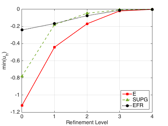
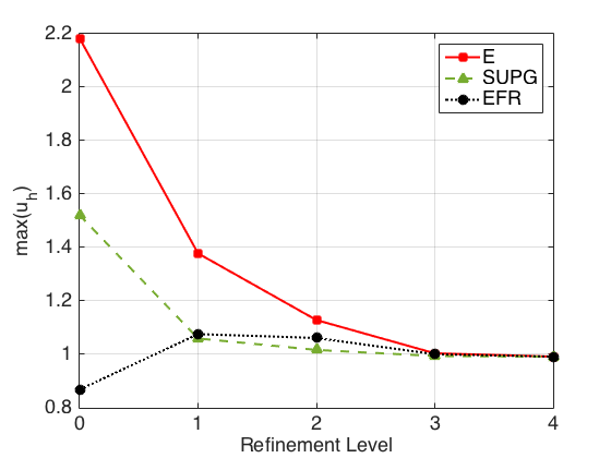
Figure 2: Minimum value (left) and maximum value (right) of the solution at $t=0.5$ computed by the standard Galerkin method (E), the SUPG method, and the EFR method with $\delta=1/n_{\ell}$, $N=0$, and $\chi=1$ plotted against the refinement level.

Next, we focus on the EFR algorithm and vary the order of the deconvolution $N$. In Fig. 3 (left) we show $L^{2}$ and $H^{1}$ norms of the error for $u$ at $t=0.5$ given by the EFR method with $\delta=1/n_{\ell}$ and $N=0,1,2,3$ plotted against the refinement level. The only visible difference when $N$ varies is for the finer meshes, with both errors slightly decreasing as $N$ is increased. Fig. 3 (right) displays a zoomed-in view of Fig. 3 (left) around $\ell=0,1$. It shows that also for the coarser meshes the errors get slightly smaller when $N$ increases. We recall that indicator function (16) with $D=D_{N}$ requires to apply the Helmholz filter $N+1$ times. So, the slightly smaller errors for large $N$ come with an increased computational time.

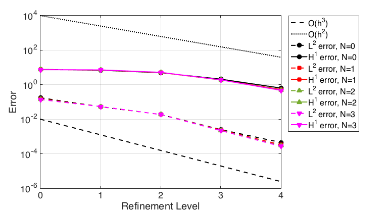
Figure 3: Left: $L^{2}$ and $H^{1}$ norms of the error for $u$ at $t=0.5$ given by the EFR method with $\delta=1/n_{\ell}$ and $N=0,1,2,3$ plotted against the refinement level. Right: zoomed-in view around $\ell=0,1$.

In Fig. 4, we report the indicator function at $t=0.5$ for $\delta=1/n_{\ell}$ and $N=0,1,2,3$. In all the cases, the largest values of the indicator function are around the edge of the hump. Moderate values are aligned with the direction of ${\bf b}$. While we see some differences in the indicator functions for $N=0$ and $N=1$, for $N>1$ the indicator function does not seem to change substantially.

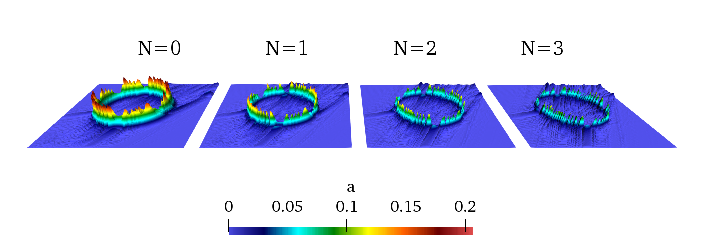
Figure 4: Indicator function on mesh $\ell=2$ at $t=0.5$ for $\delta=1/n_{\ell}$ and $N=0,1,2,3$.

Finally, we fix $N=0$ and vary $\delta$. In Fig. 5 (left) we show $L^{2}$ and $H^{1}$ norms of the error for $u$ at $t=0.5$ given by the EFR method with $\delta=c/n_{\ell}$, $c=1,\sqrt{2},2,5$, plotted against the refinement level. Notice that $c=\sqrt{2}$ corresponds to the choice $\delta=h$, while $c=1$ corresponds to $\delta=h_{min}$. In BQV , it was found that $\delta=h_{min}$ makes the numerical results (for a Navier-Stokes problem on unstructured meshes) in better agreement with experimental data. Our results confirm that $\delta=h_{min}$ is the best choice. In fact, it minimizes the error and gives optimal convergence rates. Higher values of $c$, i.e. $c>1$, seem to spoil the convergence rate of the EFR method. From Fig. 3 (left) and 5 (left) we see that the computed solution is much more sensitive to $\delta$ than it is to $N$. Fig. 5 (right) shows the solution at time $t=0.5$ computed by the EFR method with $\delta=5/n_{\ell}$ on mesh $\ell=0$. Remember that $\delta$ is the filtering radius, i.e. the radius of the circle over which we average (in some sense) the solution. Thus, it is not surprising that for a large value of $\delta$ the EFR method has an over-smoothing effect.

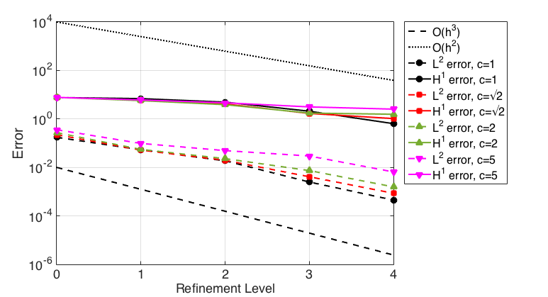
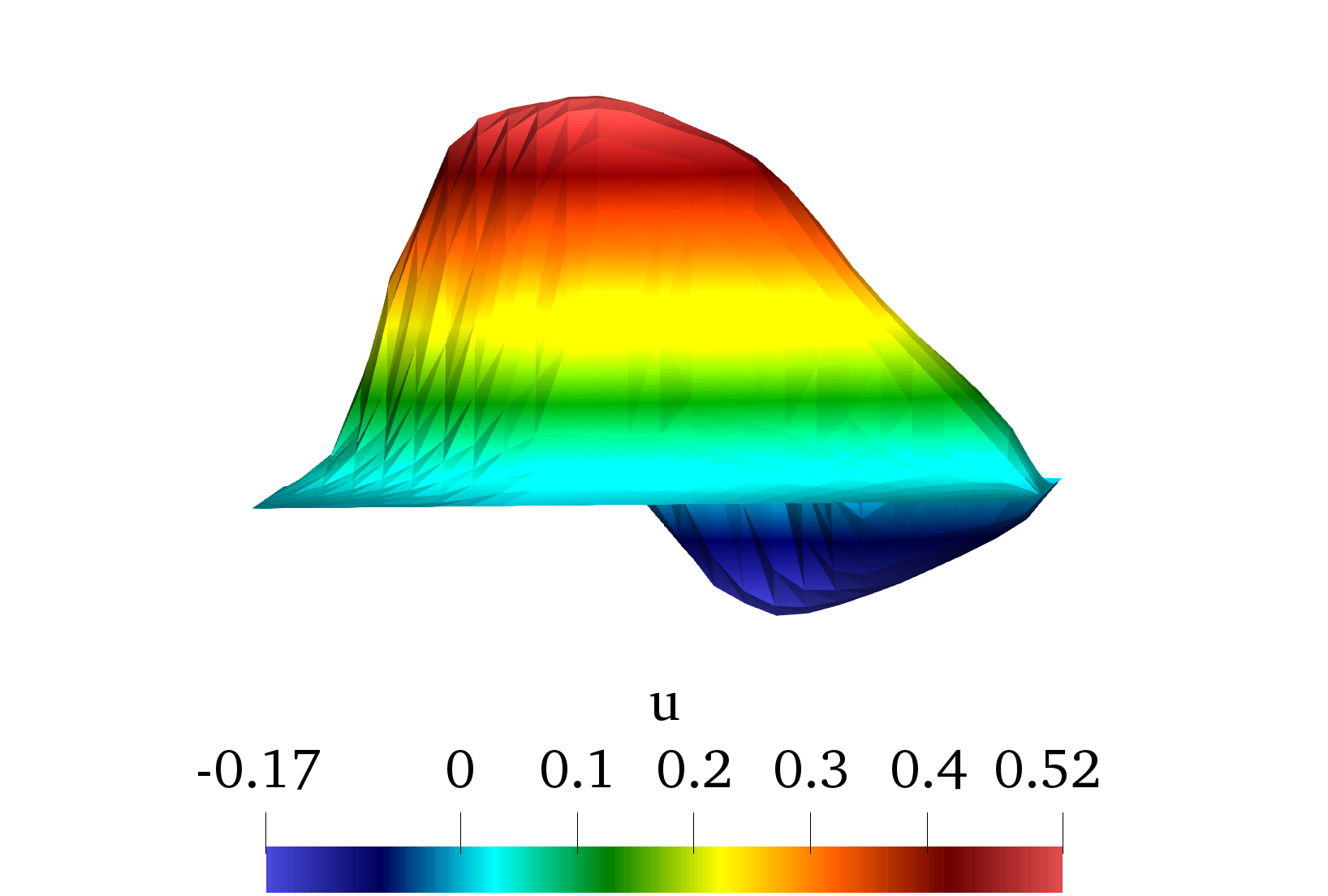
Figure 5: Left: $L^{2}$ and $H^{1}$ norms of the error for $u$ at $t=0.5$ given by the EFR method with $N=0$ and $\delta=c/n_{\ell}$, $c=1,\sqrt{2},2,5$, plotted against the refinement level. Right: solution at $t=0.5$ computed by the EFR method with $\delta=5/n_{\ell}$ on mesh $\ell=0$.

5 Conclusions

We considered a deconvolution-based filter stabilization technique recently proposed for the Navier-Stokes equations and adapted it to the numerical solution of advection dominated advection-diffusion-reaction problems with under-refined meshes. Our stabilization technique is consistent, although not strongly. For the implementation of our approach we adopted a three-step algorithm called evolve-filter-relax (EFR) that can be easily realized within a legacy solver. We showed that the EFR algorithm is competitive when compared to classical stabilization methods on a benchmark problem that features an analytical solution. However, special care has to be taken in setting the filtering radius $\delta$ in order to avoid over-smoothing.

References

- [1] FEniCS Project. https://fenicsproject.org.
- [2] Martin S. Alnæs, Jan Blechta, Johan Hake, August Johansson, Benjamin Kehlet, Anders Logg, Chris Richardson, Johannes Ring, Marie E. Rognes, and Garth N. Wells. The fenics project version 1.5. Archive of Numerical Software, 3(100), 2015.
- [3] L. Bertagna, A. Quaini, L.G. Rebholz, and A. Veneziani. On the sensitivity to the filtering radius in Leray models of incompressible flow. In Computational Methods in Applied Sciences. Springer-ECCOMAS series, to appear.
- [4] L. Bertagna, A. Quaini, and A. Veneziani. Deconvolution-based nonlinear filtering for incompressible flows at moderately large Reynolds numbers. International Journal for Numerical Methods in Fluids, 81(8):463–488, 2016. fld.4192.
- [5] A. L. Bowers, L. G. Rebholz, A. Takhirov, and C. Trenchea. Improved accuracy in regularization models of incompressible flow via adaptive nonlinear filtering. International Journal for Numerical Methods in Fluids, 70(7):805–828, 2012.
- [6] A.L. Bowers and L.G. Rebholz. Numerical study of a regularization model for incompressible flow with deconvolution-based adaptive nonlinear filtering. Comput. Methods Appl. Mech. Eng., 258:1–12, 2013.
- [7] A.N. Brooks and T.J.R. Hughes. Streamline upwind/Petrov-Galerkin formulations for convection dominated flows with particular emphasis on the incompressible Navier-Stokes equation. Comput. Methods Appl. Mech. Engrg., 32:199–259, 1982.
- [8] R. Codina. Comparison of some finite element methods for solving the diffusion-convection-reaction equation. Comput. Methods Appl. Mech. Engrg., 156:185–210, 1998.
- [9] Ramon Codina. A discontinuity-capturing crosswind-dissipation for the finite element solution of the convection-diffusion equation. Computer Methods in Applied Mechanics and Engineering, 110(3):325 – 342, 1993.
- [10] P.A.B. de Sampaio and A.L.G.A. Coutinho. A natural derivation of discontinuity capturing operator for convection-diffusion problems. Computer Methods in Applied Mechanics and Engineering, 190(46):6291 – 6308, 2001.
- [11] J. Douglas and J. Wang. An absolutely stabilized finite element method for the Stokes problem. Math. Comp., 52:495–508, 1989.
- [12] A. Dunca and Y. Epshteyn. On the Stolz-Adams deconvolution model for the large-eddy simulation of turbulent flows. SIAM J. Math. Anal., 37(6):1980–1902, 2005.
- [13] Vincent J. Ervin, William J. Layton, and Monika Neda. Numerical analysis of filter-based stabilization for evolution equations. SIAM Journal on Numerical Analysis, 50(5):2307–2335, 2012.
- [14] M. Germano. Differential filters of elliptic type. Phys. of Fluids, 29:1757–1758, 1986.
- [15] Thomas J.R. Hughes and Michel Mallet. A new finite element formulation for computational fluid dynamics: Iv. a discontinuity-capturing operator for multidimensional advective-diffusive systems. Computer Methods in Applied Mechanics and Engineering, 58(3):329 – 336, 1986.
- [16] T.J.R. Hughes. Multiscale phenomena: Green’s function, the Dirichlet-to-Neumann formulation, subgrid scale models, bubbles and the origins of stabilized formulations. Comput. Methods Appl. Mech. Engrg., 127:387–401, 1995.
- [17] T.J.R. Hughes and A.N. Brooks. A multidimensional upwind scheme with no crosswind diffusion. In T.J.R. Hughes, editor, FEM for Convection Dominated Flows. ASME, New York, 1979.
- [18] T.J.R. Hughes, L.P. Franca, and G.M. Hulbert. A new finite element formulation for computational fluid dynamics: VIII. The Galerkin / least-squares method for advective-diffusive equations. Comput. Methods Appl. Mech. Engrg., 73:173–189, 1989.
- [19] J.C. Hunt, A.A. Wray, and P. Moin. Eddies stream and convergence zones in turbulent flows. Technical Report CTR-S88, CTR report, 1988.
- [20] Volker John and Ellen Schmeyer. Finite element methods for time-dependent convection–diffusion–reaction equations with small diffusion. Computer Methods in Applied Mechanics and Engineering, 198(3):475 – 494, 2008.
- [21] D. Kuzmin. A Guide to Numerical Methods for Transport Equations. University Erlangen-Nuremberg, Erlangen, 2010.
- [22] W. Layton, L.G. Rebholz, and C. Trenchea. Modular nonlinear filter stabilization of methods for higher Reynolds numbers flow. J. Math. Fluid Mech., 14:325–354, 2012.
- [23] Anders Logg, Kent-Andre Mardal, Garth N. Wells, et al. Automated Solution of Differential Equations by the Finite Element Method. Springer, 2012.
- [24] A. Quarteroni and A. Valli. Numerical Approximation of Partial Differential Equations. Springer-Verlag, 1994.
- [25] A.W. Vreman. An eddy-viscosity subgrid-scale model for turbulent shear flow: Algebraic theory and applications. Physics of Fluids, 16(10):3670–3681, 2004.
- [26] Huijuan Xu, Marina Piccinelli, Bradley G. Leshnower, Adrien Lefieux, W. Robert Taylor, and Alessandro Veneziani. Coupled morphological–hemodynamic computational analysis of type b aortic dissection: A longitudinal study. Annals of Biomedical Engineering, Mar 2018.