A systematic approach to determine the spectral characteristics of molecular magnets

Abstract

We devise a formalism to investigate in a systematic way the spectroscopic magnetic excitations in molecular magnets. This consists in introducing a bilinear spin Hamiltonian that allows for discrete coupling parameters accounting for distinct spin coupling mechanisms among the constituent magnetic ions, as well as the influence of the nonmagnetic ions in the system. The model is applied to explore the magnetic excitations of the trimeric magnetic compounds $\mathrm{A_{3}Cu_{3}(PO_{4})_{4}}$  $\mathrm{(A\ =\ Ca,\ Sr,\ Pb)}$ and the tetrameric molecular magnet $\mathrm{Ni_{4}Mo_{12}}$. Our results are in a very good agreement with the available experimental data: For all trimers $\mathrm{A_{3}Cu_{3}(PO_{4})_{4}}$, calculations reveal the existence of one thin energy band referring to the flatness of observed excitation peaks. Moreover for the tetramer $\mathrm{Ni_{4}Mo_{12}}$, we concluded that the magnetic excitations may be traced back to the specific geometry and complex chemical structure of the exchange bridges leading to the splitting and broadness of the peaks centered about 0.5 meV and 1.7 meV.

I Introduction

Molecular nanomagnets have seen a resurgence of interest in recent years (for an extensive review see e.g. Ref. Sieklucka and Pinkowicz (2017) and references therein). Their small size allows precise characterizability both theoretically and experimentally. They possess unique properties and are ideal candidates for exploring the interplay of the quantum and the classical worlds. Their magnetic properties are determined from the collective behavior of weakly interacting fundamental structural units forming isolated dimers, trimers and tetramers Furrer and Waldmann (2013). They have great potential for technological applications: The effect of quantum tunnelling in single-molecule magnets Wernsdorfer et al. (2002); Schenker et al. (2005), the response of spin-switching in the frustrated antiferromagnetic chromium trimmer Jamneala et al. (2001) and even-odd effects in spin chain magnets Machens et al. (2013) are some prominent examples. Furthermore, the molecular magnet $\mathrm{Ni_{4}Mo_{12}}$ provides a unique opportunity for exploring unusual magnetic behavior Schnack et al. (2006); Kostyuchenko (2007), while the difference in the magnetic properties Ghosh et al. (2010a) among the compounds $\mathrm{Ca_{3}Cu_{2}Ni(PO_{4})_{4}}$ and $\mathrm{Ca_{3}Cu_{2}Mg(PO_{4})_{4}}$ shows the richness of the physical features of linear spin trimers (see e.g. Ghosh et al. (2010b); Ghosh and Ghoshray (2012)). It is worth mentioning that even the structure of the nucleon and the distribution of its spin degrees of freedom are not yet fully understood Aidala et al. (2013) signalling the continuous scientific interest in exploring the features of the “smallest” quantum spin systems. Whether in nuclear physics or in solids these systems play an important role for testing theoretical formalisms. The nature of the underlying quantum collective processes such as higher order spin exchange interactions can be analysed in terms of different spin Hamiltonians Coldea et al. (2001); Zaharko et al. (2008); Islam et al. (2010); Klemm and Efremov (2008); Gatteschi et al. (2006). Within the nature of spin exchange processes nanomagnets can be studied also in the context of quantum estimation theory Troiani and Paris (2016). Theoretical analysis of molecular magnets $\mathrm{Fe_{8}}$ and $\mathrm{Mn_{12}}$ based on the Grover algorithm Leuenberger and Loss (2001), makes them promising candidates for building memory devices. Moreover the heterometallic linkers $\mathrm{Cr_{7}Ni}$ molecular rings were used to investigate the propagation of spin information at the supramolecular scale Bellini et al. (2011).

Magnetic molecules possess intrinsic properties and are ideal systems to gain useful insights into the underlying coupling mechanisms. On the experimental side, Inelastic Neutron Scattering (INS) Lovesey (1986); Collins (1989); Furrer et al. (2009); Toperverg and Zabel (2015) plays a central role in determining the exchange effects and relevant magnetic spectra. In complement to different magnetic measurment methods, INS techniques appear to be of high value, and in the past decades it has been widely applied to explore the properties of spin clusters. INS experiments on the spin dimer $[\text{Ni}_{2}(\text{ND}_{2}\text{C}_{2}\text{H}_{4}\text{ND}_{2})_{4}\text{Br}_{2}]\text{Br}_{2}$ has demonstrated the important contribution of neutron spectroscopy Stebler et al. (1982). INS measurments were obtained for different magnetic clusters, such as: The trimer $\mathrm{La_{4}Cu_{3}MoO_{12}}$, with strong intratrimer antiferromagnetic interactions, where the copper ions form an isolated triangle Azuma et al. (2000), the dimer $\text{SrCu}_{2}(\text{BO}_{3})_{2}$ with observed multiplet excitations Kageyama et al. (2000); Gaulin et al. (2004) the polyoxomolybdate $\text{Mn}_{72}\text{Fe}_{32}$ Garlea et al. (2006), and the magnetic molecule Fe₉ in presence of an external magnetic field Vaknin and Demmel (2014).

The physical properties, such as energy spectra, susceptibility, etc., of magnetic clusters at the nanoscale depend on their size, shape (for more details see Chamati (2013); Sellmyer et al. (2015); Sieklucka and Pinkowicz (2017) and references therein) and the presence of different bondings among the constituent chemical elements. Thus the distribution of ligands with different strength in conjunction with finite-size, as well as surface effects have huge impact on their characteristics.

When studying the spectral properties of single magnetic molecules, usually (see e.g. Ref. Furrer and Waldmann (2013) and references therein) one relies on the structural symmetry of the cluster to solve the ensuing quantum mechanical problem. Thus grouping symmetrically equivalent spins into a resulting single one employing the sum rules of angular momenta. Further one adds more spins according to well defined selection rules till fully characterizing the specific cluster under consideration.

The main aim of the present paper is to propose an alternative approach that leads naturally to computing the relevant physical quantities of any magnetic cluster. Furthermore, it is able to reproduce reasonably well the experimental results. The present approach is based on the assumption that in a molecular magnet with nontrivial geometry and complex chemical environment neither the exchange path between two magnetic ions nor the corresponding coupling are unique. This causes the transition energy to vary, leading to a broadened excitation width in the energy spectrum and even splitting. Accordingly the number of all energy values form a set that can uniquely identify the most relevant bonds, despite being identical to each other. The associated effect could be studied by accounting for appropriate spin coupling parameters. To this end, we introduce a bilinear microscopic spin Hamiltonian with discrete couplings that allow for distinct spin coupling mechanisms among equivalent spins allowing one to identify the different exchange paths. Hence, one can precisely determine the energy levels and the relevant magnetic characteristics of magnetic clusters and the underlying physical processes of experimentally observed spectra.

The present method is powerful and quite general. It can be applied to a variety of physical problems, such as unveiling the structure of the nucleus (see e.g. Ref. Thomas (2008)). Here, it will be tested on two classes of molecular magnets that have generated a great deal of interest by many researchers both on the theoretical as well as the experimental sides.

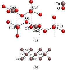
Figure 1: (a) Exchange pathways in $\mathrm{A_{3}Cu_{3}(PO_{4})_{4}}$ $(\mathrm{A=Ca,Sr,Pb})$. Copper colored circles represent copper ions, the red ones stand for oxygen atoms. The solid (black) and dashed (gray) lines represent the intratrimer and intertrimer exchange pathways, respectively. (b) Schematic representation of the intratrimer $J$ and intertrimer $J^{\prime}$ magnetic interactions in the array of isolated trimers.

The first class of materials that are the focus of our attention belongs to the family of compounds $\mathrm{A_{3}Cu_{3}(PO_{4})_{4}}$ with $\mathrm{(A=Ca,Sr,Pb)}$, where the three spin-half $\mathrm{Cu^{2+}}$ ions form a linear trimer (see FIG. 1). Magnetic measurements on trimer copper chains with $\mathrm{(A=Ca,Sr)}$ are reported in Ref. Drillon et al. (1993) and analysed in the framework of Heisenberg and Ising models. It was shown that the intertrimer interactions are negligible and thus the trimers might be considered as separate clusters. These results were confirmed via INS experiments Matsuda et al. (2005); Podlesnyak et al. (2007) that shed light on the magnetic spectra with the aid of the antiferromagnetic Heisenberg model involving nearest and next-nearest intratrimer interactions, and later they were extended to the compound $\mathrm{Ca_{3}Cu_{3}(PO_{4})_{4}}$ Furrer (2010). Moreover, it turns out that the interaction between edge spins in the isolated trimer is also negligible.

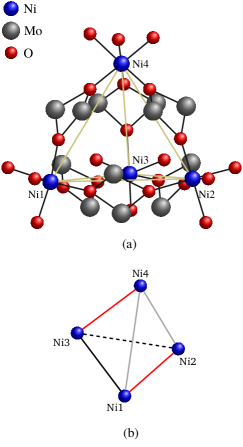
Figure 2: (a) Sketch of the structure of the molecular nanomagnet Ni₄Mo₁₂. (b) Schematic view of the arrangment of Ni ions (blue balls). The grey lines represent the two shorter distances, while the red lines show the spin-1 dimers.

The second material of interest is the magnetic molecule $[\mathrm{Mo_{12}O_{30}(\mu_{2}-OH)_{10}H_{2}(Ni(H_{2}O)_{3})_{4}}]$, denoted by $\mathrm{Ni_{4}Mo_{12}}$, where four spin-1 $\mathrm{Ni^{2+}}$ ions are sitting on the vertices of a distorted tetrahedron (see FIG. 2). This molecule shows an unusual magnetic behavior Schnack et al. (2006). It was suggested Kostyuchenko (2007) that the experimental data could be explained by accounting for a three interaction term in addition to the Heisenberg nearest-neighbor exchange and a biquadratic term. The theoretical description of INS data, especially the intensity and the width of the peak at about $1.7\ \textrm{meV}$ has attracted lot of interest (for more details see Ref. Nehrkorn et al. (2010) and references therein). In Ref. Furrer et al. (2010) it was pointed out that the Heisenberg model with single-ion anisotropy is a Hamiltonian adequate to reproduce the main features of experimentally obtained INS data. However, even by including higher order terms and/or perturbations, such as single-ion anisotropy an accurate reproduction of the experimental INS spectrum is not yet reported.

The rest of this paper is structured as follows: In Section II we present the details of our approach and its advantages when applied to spin systems. We formulate explicitly the Hamiltonian and the key constraints that allow the derivation of the main results throughout the rest of paper. In Sections III and IV we explore the low-lying magnetic excitations of the compounds $\mathrm{A_{3}Cu_{3}(PO_{4})_{4}}$ (where A stands for Ca, Sr, Pb) and $\mathrm{Ni_{4}Mo_{12}}$. A summary of the results obtained throughout this paper are presented in Section V.

II The model and the method

II.1 INS and the Heisenberg model

The study of magnetic excitations determined by INS techniques on one hand requires a specific microscopic model, and on the other an analysis of the neutron scattering probabilities Lovesey (1986); Collins (1989); Furrer et al. (2009); Toperverg and Zabel (2015). To determine the energy level structure and the transitions corresponding to the experimentally observed magnetic spectra one needs a minimal number of parameters to account for all couplings in the system. It is cumbersome to apply a general approach with a unique set of parameters that can describe all possible magnetic effects and in addition to distinguish between inter-molecular and intra-molecular features. The principal assumption of our method is that the magnetic excitations of spin clusters obtained by INS are mainly governed by the exchange of electrons between the constituent ions. Then, the experimental data are interpreted in terms of a well defined microscopic model. In the absence of anisotropy, i.e. negligible spin-orbit coupling, the exchange interaction in molecular magnets can be described by the Heisenberg model

$$\hat{H}=\sum\limits_{i\neq j}J_{ij}\hat{\mathbf{s}}_{i}\cdot\hat{\mathbf{s}}_{j},$$ (1)

where $J_{ij}=J_{ji}$ is the exchange coupling that effectively accounts for the electrostatic interaction between the $i$th and $j$th ions and represents the amount of transition energy arising due to the electron’s spins. Hamiltonian (1) commutes with the square and each component of the total spin operator $\hat{\mathbf{s}}=\sum_{i}\hat{\mathbf{s}}_{i}$. Therefore the eigenvalues of Hamiltonian (1) can be computed within the total spin operator eigenstates $\rvert s,m\rangle$, where $s$ and $m$ stand for the total spin and magnetic quantum numbers, respectively.

Depending on the geometry of the specific cluster under consideration, other magnetic and non-magnetic properties may be taken into account by generalizing the Hamiltonian (1). The general practice is to include different interaction terms referring to the type of exchange under consideration. Such terms are biquadratic Blume and Hsieh (1969); Penc and Läuchli (2011); Smerald and Shannon (2013), four-spin Ivanov et al. (2009); Müller et al. (2002); Läuchli et al. (2005), three-body Ivanov et al. (2014); Michaud and Mila (2013) or high order multipolar interaction terms Santini et al. (2009). Even with some of the aforementioned interactions the eigenvalues of the ensuing Hamiltonian may remain degenerates with respect to the total magnetic quantum number, leaving the experimentally observed splitting effects of the magnetic spectrum unexplained. Furthermore, the interplay between the different terms may break the rotational symmetry and the total spin $s$ may no longer be a good quantum number. Moreover one may include perturbation terms like the single-ion anisotropy which arises due to the one site spin-orbit coupling Rudowicz and Karbowiak (2015).

The identification of the experimentally observed magnetic peaks in the obtained energy level structure, estimated by the considered microscopic model, is not unique. To obtain meaningful results one has to calculate the scattering intensities $I_{n^{\prime}n}(\mathbf{q})$, integrated over the angles of the scattering vector $\mathbf{q}$, of the existing transitions and analyse their dependence on the temperature and the magnitude of the neutron scattering vector. For identical magnetic ions, we have Lovesey (1986); Collins (1989); Furrer et al. (2009); Toperverg and Zabel (2015)

$$I_{n^{\prime}n}(\mathbf{q})\propto F^{2}(\mathrm{q})\sum_{\alpha,\beta}\varTheta^{\alpha\beta}S^{\alpha\beta}(\mathbf{q},\omega_{n^{\prime}n}).$$ (2)

Here $\mathbf{q}=\mathbf{k}_{0}-\mathbf{k}$, with $\mathbf{k}_{0}$ and $\mathbf{k}$ – the incoming and the scattered neutron wave vectors, respectively. The magnitudes of these vectors are denoted by $\mathrm{q}$, $k_{0}$ and $k$. The transition’s frequency, with neutron’s mass $\mu$, is given by $\omega=(2\mu)^{-1}(\mathbf{k}^{2}-\mathbf{k}^{2}_{0})$, $F(\mathrm{q})$ – the spin magnetic form factor, $\varTheta^{\alpha\beta}$ is the polarization factor, and $\alpha,\beta,\gamma\in\{x,y,z\}$. In (2) the magnetic scattering functions are explicitly written as

$$S^{\alpha\beta}(\mathbf{q},\omega)= \ \sum_{n,n^{\prime},i,j}e^{\mathrm{i}\mathbf{q}\cdot\mathbf{r}_{ij}}p_{n}\langle n\lvert\hat{s}^{\alpha}_{i}\rvert n^{\prime}\rangle\langle n^{\prime}\rvert\hat{s}^{\beta}_{j}\rvert n\rangle\,\delta(\hbar\omega-E_{n^{\prime}n}),$$ (3)

$$\quad p_{n}=Z^{-1}e^{-\frac{E_{n}}{k_{B}T}},$$

where $\rvert n\rangle$, $\rvert n^{\prime}\rangle$ are the initial and final states with the corresponding energy $E_{n}$ and $E_{n^{\prime}}$, respectively, $E_{n^{\prime}n}(=E_{n^{\prime}}-E_{n})$ – the transition energy and $Z$ is the partition function. The term $e^{\mathrm{i}\mathbf{q}\cdot\mathbf{r}_{ij}}$ is the structure factor associated with the cluster geometry. When $s$ is a good quantum number the eigenstates $\rvert n\rangle\equiv\ \rvert s,m\rangle$ and $\rvert n^{\prime}\rangle\equiv\ \rvert s^{\prime},m^{\prime}\rangle$, where $s$ and $m$ stand for the total spin and magnetic quantum numbers, respectively. Therefore, a magnetic transition sets in when $\omega\equiv\omega_{n^{\prime}n}$.

The spin magnetic form factor Jensen and Mackintosh (1991) is given by

$$F(\mathrm{q})=\int\limits_{0}^{\infty}\mathrm{r}^{2}R^{2}_{i0}(\mathrm{r})J_{\nu}(\mathrm{q},\mathrm{r})\mathrm{d}\mathrm{r},$$ (4)

where $R_{i0}(\mathrm{r})$ are the radial wave functions and $J_{\nu}(\mathrm{q},\mathrm{r})$ are the spherical Bessel functions of the first kind. The advantage of INS is that one can clearly distinguish the magnetic transitions from phonon excitations, as the former obey different statistics and decrease by increasing the magnitude of scattering vector. Furthermore, this method does not require an external magnetic field, since the neutron spin interacts with the intrinsic magnetic field of the cluster.

II.2 Phenomenological spin model

In molecular magnets, the distribution of coupled spins (dimers) plays a crucial role in uniquely determining the scattering intensities. Even when the bonds are indistinguishable with respect to their lengths and the total spin of the coupled spins, according to (3), one can clearly obtain different in magnitude neutron scattering intensities. However, to distinguish the intensities one has to use an appropriate spin model leading to an energy sequence such that the $\delta$ function in the r.h.s of (3) identifies the spin bonds with respect to the structure factors. Notice that, even with a selected a priori spin coupling scheme, the Hamiltonian (1) may not be adequate to obtain the correct energy structure.

In the quest of a procedure that allows to characterize uniquely each bond in a magnetic cluster assuming nonuniqueness of exchange pathways we propose the following Hamiltonian

$$\hat{\mathcal{H}}=\sum\limits_{i\neq j}J_{ij}\hat{\boldsymbol{\sigma}}_{i}\cdot\hat{\mathbf{s}}_{j},$$ (5)

where the couplings $J_{ij}=J_{ji}$ are effective exchange constants and the operator $\hat{\boldsymbol{\sigma}}_{i}\equiv(\hat{\sigma}^{x}_{i},\hat{\sigma}^{y}_{i},\hat{\sigma}^{z}_{i})$ accounts for the differences in local coupling processes of the $i$-th ion. If $J_{ij}$ is not indentical for all pairs $i$ and $j$, then the sigma operators will differ from their associated spin operators. This will allow one to obtain the whole set of transition energies corresponding to the exchange between $i$th and $j$th ions.

For a single spin the square and $z$ component of each operator $\sigma$ are completely determined in the basis of the total spin component $\hat{s}^{z}$, such that for all $i$ and $\alpha\in\{x,y,z\}$

$$\hat{\sigma}^{\alpha}_{i}\lvert\ldots,s_{i},m_{i},\ldots\rangle=a^{s_{i},m_{i}}_{i}\hat{s}^{\alpha_{\phantom{i}}}_{i}\lvert\ldots,s_{i},m_{i},\ldots\rangle,$$ (6)

where $a^{s_{i},m_{i}}_{i}\in\mathbb{R}$. Furthermore, the $\sigma$ rising and lowering operators obey the equations

$$\hat{\sigma}^{\pm}_{i}\lvert\ldots,s_{i},m_{i},\ldots\rangle=a^{s_{i},m_{i}}_{i}\hat{s}^{{\pm}_{\phantom{i}}}_{i}\lvert\ldots,s_{i},m_{i},\ldots\rangle.$$ (7)

For all $i$, the square of $\sigma_{i}$ commutes only with its $z$ component. Its eigenvalues depend on $m_{i}$ and according to (6) and (7) one can distinguish three cases: (1) $m_{i}=s_{i}$; (2) $-s_{i}<m_{i}<s_{i}$ and (3) $m_{i}=-s_{i}$, where $s_{i}\neq 0$, with the respective eigenvalues

$$\left(a^{s_{i},s_{i}}_{i}\right)^{2}s^{2}_{i}+a^{s_{i},s_{i}}_{i}a^{s_{i},s_{i}-1}_{i}s_{i},$$ (8a)

$$\tfrac{1}{2}a^{s_{i},m_{i}}_{i}\left[a^{s_{i},m_{i}+1}_{i}+a^{s_{i},m_{i}-1}_{i}\right]s_{i}(s_{i}+1)+\left(a^{s_{i},m_{i}}_{i}\right)^{2}m^{2}_{i}$$

$$-\tfrac{1}{2}a^{s_{i},m_{i}}_{i}m_{i}\left[a^{s_{i},m_{i}+1}_{i}(m_{i}+1)+a^{s_{i},m_{i}-1}_{i}(m_{i}-1)\right],$$ (8b)

$$\left(a^{s_{i},-s_{i}}_{i}\right)^{2}s^{2}_{i}+a^{s_{i},-s_{i}}_{i}a^{s_{i},1-s_{i}}_{i}s_{i}.$$ (8c)

On the other hand when the spins of $i$th and $j$th magnetic ions are coupled, with total spin operator $\hat{\mathbf{s}}_{ij}=\hat{\mathbf{s}}_{i}+\hat{\mathbf{s}}_{j}$, the relation (6) enters a more general and complex expression. To explore the properties of the coupled spins one has to work with the total $\sigma$-operator $\hat{\boldsymbol{\sigma}}_{ij}$. Its $z$ component and square are completely determined in the basis of the spin operator $\hat{\mathbf{s}}^{2}_{ij}$. Similar to Eq. (6) for all $i\neq j$ and $\alpha\in\{x,y,z\}$, we have

$$\hat{\sigma}^{\alpha}_{ij}\lvert\ldots,s_{ij},m_{ij},\ldots\rangle=a^{s_{ij},m_{ij}}_{ij}\hat{s}^{\alpha_{\phantom{j}}}_{ij}\lvert\ldots,s_{ij},m_{ij},\ldots\rangle,$$ (9)

where $a^{s_{ij},m_{ij}}_{ij}\in\mathbb{R}$. The corresponding rising and lowering operators obey

$$\hat{\sigma}^{\pm}_{ij}\lvert\ldots,s_{ij},m_{ij},\ldots\rangle=a^{s_{ij},m_{ij}}_{ij}\hat{s}^{{\pm}_{\phantom{i}}}_{ij}\lvert\ldots,s_{ij},m_{ij},\ldots\rangle.$$ (10)

The eigenvalues of $\hat{\boldsymbol{\sigma}}^{2}_{ij}$ depend on $m_{ij}$. Therefore having in mind the following three cases $m_{ij}=s_{ij}$, $-s_{ij}<m_{ij}<s_{ij}$ and $m_{ij}=-s_{ij}$, where $s_{ij}\neq 0$ the eigenvalues read

$$\left(a^{s_{ij},s_{ij}}_{ij}\right)^{2}s^{2}_{ij}+a^{s_{ij},s_{ij}}_{ij}a^{s_{ij},s_{ij}-1}_{ij}s_{ij},$$ (11a)

$$\tfrac{1}{2}a^{s_{ij},m_{ij}}_{ij}\left[a^{s_{ij},m_{ij}+1}_{ij}+a^{s_{ij},m_{ij}-1}_{ij}\right]s_{ij}(s_{ij}+1)+\left(a^{s_{ij},m_{ij}}_{ij}\right)^{2}m^{2}_{ij}$$

$$-\tfrac{1}{2}a^{s_{ij},m_{ij}}_{ij}m_{ij}\left[a^{s_{ij},m_{ij}+1}_{ij}(m_{ij}+1)+a^{s_{ij},m_{ij}-1}_{ij}(m_{ij}-1)\right],$$ (11b)

$$\left(a^{s_{ij},-s_{ij}}_{ij}\right)^{2}s^{2}_{ij}+a^{s_{ij},-s_{ij}}_{ij}a^{s_{ij},1-s_{ij}}_{ij}s_{ij}.$$ (11c)

The corresponding $\sigma$-operators share a single coefficient and for $i\neq j$ and $\alpha\in\{x,y,z\}$, we have

$$\hat{\sigma}^{\alpha}_{i}\lvert\ldots,s_{ij},m_{ij},\ldots\rangle=a^{s_{ij},m_{ij}}_{ij}\hat{s}^{\alpha_{\phantom{j}}}_{i}\lvert\ldots,s_{ij},m_{ij},\ldots\rangle.$$ (12)

We further assume that the $\sigma$-operators preserve the corresponding spin magnetic moment and for a noncoupled spin obey the following constraints

$$\hat{\sigma}^{z}_{i}\lvert\ldots,s_{i},m_{i},\ldots\rangle=m_{i}\lvert\ldots,s_{i},m_{i},\ldots\rangle,$$ (13a)

$$\hat{\boldsymbol{\sigma}}^{2}_{i}\lvert\ldots,s_{i},m_{i},\ldots\rangle=s_{i}(s_{i}+1)\lvert\ldots,s_{i},m_{i},\ldots\rangle.$$ (13b)

Similarly, when the $i$th and $j$th spins are coupled, for all $i\neq j$ we have

$$\hat{\sigma}^{z}_{ij}\lvert\ldots,s_{ij},m_{ij},\ldots\rangle=m_{ij}\lvert\ldots,s_{ij},m_{ij},\ldots\rangle,$$ (14a)

$$\hat{\boldsymbol{\sigma}}^{2}_{ij}\lvert\ldots,s_{ij},m_{ij},\ldots\rangle=s_{ij}(s_{ij}+1)\lvert\ldots,s_{ij},m_{ij},\ldots\rangle.$$ (14b)

Taking into account (13) together with expressions (8) for all $i$ we have

$$\begin{array}[]{c}a^{s_{i},m_{i}\pm 1}_{i}=a^{s_{i},m_{i}}_{i}=1\quad\forall\ m_{i}\neq 0,\\[2.84544pt] a^{s_{i},m_{i}\pm 1}_{i}=a^{s_{i},0}_{i}=\pm 1.\end{array}$$ (15)

Further, according to constraints (14) and Eqs. (11) we distinguish three cases:

(1) $s_{ij}\neq 0$, $m_{ij}\neq 0$: Then

$$a^{s_{ij},m_{ij}\pm 1}_{ij}=a^{s_{ij},m_{ij}}_{ij}=1.$$

As a result the transformations of eigenvectors via the $\sigma$-operator coincide with those defined by its corresponding spin operator. Therefore, all couplings will be constants and the Hamiltonian (5) will capture the same features as its Heisenberg parent.

(2) $s_{ij}\neq 0$ and $m_{ij}=0$: The corresponding coefficient cannot be determined from Eq. (14a) and from Eqs. (11) and (14b) one obtains

$$a^{s_{ij},m_{ij}\pm 1}_{ij}=a^{s_{ij},0}_{ij}=\pm 1.$$ (16)

We would like to point out that the “minus” sign is an intrinsic feature of the sigma operators and is not related to the effectively accounted for spatial part of the wave function.

(3) $s_{ij}=0$: The associated parameter remains unconstrained and there exist a set of coefficients $c^{n}_{ij}\in\mathbb{R}$ $\forall n\in\mathbb{N}$, such that

$$a^{0,0}_{ij}\in\{c^{n}_{ij}\}_{n\in\mathbb{N}}.$$ (17)

The values of $c^{n}_{ij}$ are indirect measures for the field strength along each possible exchange pathway and therefore the changes in the energy of exchange. Depending on the type of exchange these effective coefficients are functions of the Coloumb, hopping and exchange integrals. Thus, one can expect the emergence of bands in the energy spectrum, associated with the existence of more then one exchange pathway between magnetic ions leading to a broadened excitation width of the transition energy. Thereby, for a linear cluster with only one bonding anion between magnetic cations one would obtain the limit $|c^{n}_{ij}-c^{k}_{ij}|\to 0,\ \forall\ n\neq k$, where $c^{n}_{ij}\to 1$. Accordingly, the changes in the exchange field could be considered as negligible pointing to sharpened peaks in the magnetic spectrum. On the other hand, the inequality $|c^{n}_{ij}-c^{k}_{ij}|>0$ for all $n\neq k$, would have to be considered as a sign for the presence of exchange paths of different energy and therefore of increased excitation width in energy. As an example, if an exchange bridge has a complex chemical structure, then one may expect that the exchange path through which the electrons hop and are exchanged is not unique. Hence, the existence of $n$ different paths can be accounted for by Hamiltonian (5), where according to (17), the transition energy $E_{ij}$ corresponding to the exchange of electrons between the $i$th and $j$th ions is written as

$$E_{ij}(c^{n}_{ij})=\tfrac{1}{2}J_{ij}(1+3c^{n}_{ij}),\qquad a^{1,0}_{ij}=1$$ (18)

and

$$E_{ij}(c^{n}_{ij})=\tfrac{1}{2}J_{ij}(3c^{n}_{ij}-1),\qquad a^{1,0}_{ij}=-1.$$ (19)

Thus, the set of values $E_{ij}(c^{n}_{ij})$ will correspond to a broadened peaks in the magnetic spectrum. Since $E_{ij}(c^{n}_{ij})=2J_{c^{n}_{ij}}$, where $J_{c^{n}_{ij}}$ is the $n$-th value of the exchange coupling from (18) and (19) we respectively obtain

$$c^{n}_{ij}=\frac{4}{3}\frac{J_{c^{n}_{ij}}}{J_{ij}}-\frac{1}{3},\qquad J_{1}=J_{ij},\ \ a^{1,0}_{ij}=1$$ (20)

and

$$c^{n}_{ij}=\frac{4}{3}\frac{J_{c^{n}_{ij}}}{J_{ij}}+\frac{1}{3},\qquad J_{5/3}=J_{ij},\ \ a^{1,0}_{ij}=-1.$$ (21)

As we will see later this approach allows one to explain the experimentally observed splitting and broadness of magnetic spectra in the molecular magnet Ni₄Mo₁₂. Furthermore, if $J_{ij}$ is restricted to nearest-neighbors, $c^{n}_{ij}$ can be used to compute the amount of energy required to observe an exchange with next-nearest neighbor ions. Thus only one coupling parameter would be necessary within the present formalism. In such case equations (20) and (21) read

$$c^{n}_{i,j+1}=\frac{4}{3}\frac{J_{c^{n}_{i,j+1}}}{J_{ij}}-\frac{1}{3},\qquad a^{1,0}_{ij}=1$$ (22)

and

$$c^{n}_{i,j+1}=\frac{4}{3}\frac{J_{c^{n}_{i,j+1}}}{J_{ij}}+\frac{1}{3},\qquad a^{1,0}_{ij}=-1,$$ (23)

respectively. The couplings $J_{c^{n}_{i,j+1}}$ will represent the exchange constant between the next-nearest neighbors. This important feature will be illustrated by determining the INS spectrum Matsuda et al. (2005) for the trimeric compound $\mathrm{Pb_{3}Cu_{3}(PO_{4})_{4}}$.

Therefore a remarkable feature of the present approach is that when the spin quantum number of coupled spins vanishes or we have at hand singlet bonds, then the relevant coefficients might be represented as either discrete or continuous quantities. With the Hamiltonian (5) the eigenvalues of all eigenstates associated to singlet bonds will be unique.

Figure 3: Energy level structure of the compounds $\mathrm{A_{3}Cu_{3}(PO_{4})_{4}}$ (A = Ca, Sr, Pb). The blue arrows show the ground state transitions, and red arrow stands for the excited transition. The energy levels corresponding to the ground state are designated by blue lines. The initial energy level of the excited transition is depicted by a red line, while by analogy to $\mathrm{Pb_{3}Cu_{3}(PO_{4})_{4}}$ the dashed red lines stand for a presumed second sub level of the excited doublet level.

III A₃Cu₃(PO₄)₄ (A = Ca, Sr and Pb)

III.1 The Hamiltonian

The magnetic compounds A₃Cu₃(PO₄)₄ (A = Ca, Sr, Pb) are convenient spin trimer systems, with spin-$\tfrac{1}{2}$ Cu²⁺, for testing the Hamiltonian (5) and studying the fundamental nature of antiferromagnetism. FIG. 1 (a) shows a small fragment of the copper ions structure with the exchange pathways relevant to oxygen atoms arrangements, where Cu2 ion is surrounded by four oxygen atoms on a plane, while Cu1 and Cu3 ions are surrounded by five oxygen atoms constructing distorted square pyramid. For brevity the other elements are not shown and only two oxygen atoms along the intratrimer Cu1–O1–Cu2 and intertrimer Cu2–O2–Cu4 pathways are labelled. In general, the exchange processes appear to be more complex and depend on the global structure of the compounds Drillon et al. (1993). Besides the superexchange interactions are sensitive Matsuda et al. (2005) to the angle between $\mathrm{Cu^{2+}}$ bonds and their lengths suggesting that the intertrimer Cu2–Cu4 interaction is much smaller than the intratrimer ones i.e. Cu1–Cu2 and Cu3–Cu2. Thus, the intertrimer exchange can be neglected and the $\mathrm{Cu^{2+}}$ sub-lattice is considered as a one-dimensional array of isolated spin trimers FIG. 1 (b).

Applying the formalism of Section II.2 by considering equations (22), (23) and taking into account that Cu1-Cu2 and Cu2-Cu3 are bonded by a single oxygen ion, we set $J_{ij}\to J_{12}=J$ and perform a study of the magnetic excitations. Owing to the trimer symmetry, Hamiltonian (5) transforms into

$$\hat{\mathcal{H}}=J\left(\hat{\boldsymbol{\sigma}}_{13}\cdot\hat{\mathbf{s}}_{2}+\hat{\boldsymbol{\sigma}}_{2}\cdot\hat{\mathbf{s}}_{13}+\hat{\boldsymbol{\sigma}}_{1}\cdot\hat{\mathbf{s}}_{3}+\hat{\boldsymbol{\sigma}}_{3}\cdot\hat{\mathbf{s}}_{1}\right).$$ (24)

With respect to Eq. (15) the total spin eigenstates are denoted by $\rvert s_{13},s,m\rangle$. Hence in contrast to the eigenvalues of (1) obtained in Refs. Furrer (2010); Machens et al. (2013); Podlesnyak et al. (2007), the eigenvalues of Hamiltonian (24) have an additional parameter that can be tuned to identify the energy of the experimentally observed third (excited) transition Matsuda et al. (2005).

III.2 Energy levels

According to (15) we have $a^{s_{2},m_{2}}_{2}=1$ for all energy levels. When the spin cluster is characterized by triplet states $\big{\lvert}1,{\tfrac{1}{2}},\pm\tfrac{1}{2}\big{\rangle}$, for all $m_{ij}$ we have $a^{1,m_{ij}}_{13}=1$. Thus, taking into account (24) we obtain the ground state energy

$$E^{\pm 1/2}_{1,1/2}=-\tfrac{3}{2}J.$$ (25)

The second pair of doublet states is associated with the first excited energy level, see FIG. 3. The edged spins of the isolated trimer are coupled in a singlet, with corresponding state $\big{\lvert}0,{\tfrac{1}{2}},\pm\tfrac{1}{2}\big{\rangle}$, i.e. $m_{13}=0$, $s_{13}=0$. Now, using (24) we end up with

$$E^{\pm 1/2}_{0,1/2}=-\tfrac{3}{2}Ja^{0,0}_{13}.$$ (26)

To fully characterize the experimentally observed transitions for $\mathrm{Pb_{3}Cu_{3}(PO_{4})_{4}}$ one requires at least three excited energy levels. Bearing in mind that the quartet level is four-fold degenerate, we deduce that the corresponding coefficient may take only two values $a^{0,0}_{13}\in\{c^{1}_{13},c^{2}_{13}\}$. Further, the observed excitations spectra Matsuda et al. (2005) are not broadened signalling that $|c^{1}_{13}-c^{2}_{13}|\approx 0$. Therefore taking into account (26) we get

$$E^{\pm 1/2}_{0,1/2}\in\left\{-\tfrac{3}{2}Jc^{1}_{13},-\tfrac{3}{2}Jc^{2}_{13}\right\}.$$

Furthermore, in the quartet eigenstate with all spins pointing to the same direction, $m_{13}=\pm 1$ and $m_{2}=\pm\tfrac{1}{2}$. Thus, the trimer is in the state $\big{\lvert}1,{\tfrac{3}{2}},\pm\tfrac{3}{2}\big{\rangle}$ and the energy reads

$$E^{\pm 3/2}_{1,3/2}=\tfrac{1}{2}J\left(1+a^{1,\pm 1}_{13}\right)+\tfrac{1}{2}Ja^{1,\pm 1}_{13}=\tfrac{3}{2}J.$$

For the remaining two quartet eigenstates with $m=\pm\tfrac{1}{2}$, for all $m_{ij}$ we have $a^{1,m_{ij}}_{13}=1$ thus

$$E^{\pm 1/2}_{1,3/2}=\tfrac{3}{2}J.$$

Whence, the energy sequence consists of four levels. Henceforth we denote these levels as follow

$$E_{0}=-\tfrac{3}{2}J,\quad E_{1}=-\tfrac{3}{2}Jc^{1}_{13},\quad E_{2}=-\tfrac{3}{2}Jc^{2}_{13},\quad E_{3}=\tfrac{3}{2}J.$$ (27)

III.3 Scattering intensities

The corresponding selection rules are $\Delta s_{13}=0,\pm 1$, $\Delta s=0,\pm 1$ and $\Delta m=0,\pm 1$. Calculating the scattering functions in (3) with $\lvert n\rangle\equiv\lvert s_{13},s,m\rangle$, for transitions between the energy levels, we get $S^{\alpha\beta}(\mathbf{q},\omega_{n^{\prime}n})+S^{\beta\alpha}(\mathbf{q},\omega_{n^{\prime}n})=0$, and $S^{\alpha\alpha}(\mathbf{q},\omega_{n^{\prime}n})=S^{\beta\beta}(\mathbf{q},\omega_{n^{\prime}n})$ for all $\alpha,\beta$ and $n,n^{\prime}=0,1,2,3$. Moreover, taking into account to the cluster structure, we have $\sum_{\alpha}\Theta^{\alpha\alpha}=2$. Note that due to the degeneracy of the energy spectrum with respect to $m$, for each value of $s$ and $s_{13}$ the summation over $n$ and $n^{\prime}$ in (3) corresponds to a summation over all possible values of the total magnetic quantum number. The analysis of the intensities, taking into account the experimental data, allows us to determine the observed first magnetic excitation corresponding to the transition between the ground state $\big{\lvert}1,{\tfrac{1}{2}},\pm\tfrac{1}{2}\big{\rangle}$ and the first excited states $\big{\lvert}0,{\tfrac{1}{2}},\pm\tfrac{1}{2}\big{\rangle}$ with scattering functions

$$S^{\alpha\alpha}(\mathbf{q},\omega_{20})=\tfrac{1}{3}[1-\cos(2\mathbf{q}\cdot\mathbf{r})]p_{0},$$

where $\mathbf{r}$ is the vector of the average distance between neighboring ions with $\mathbf{r}_{31}=2\mathbf{r}$. The rotational degeneracy of the quartet energy level is four–fold and hence the second ground state excitation refer to transitions from the doublet $\big{\lvert}1,{\tfrac{1}{2}},\pm\tfrac{1}{2}\big{\rangle}$ to the quartet states $\big{\lvert}1,{\tfrac{3}{2}},m\big{\rangle}$, where $m=\pm\tfrac{1}{2},\pm\tfrac{3}{2}$. Accordingly, we get

$$S^{\alpha\alpha}(\mathbf{q},\omega_{30})=\tfrac{2}{9}[3+\cos(2\mathbf{q}\cdot\mathbf{r})-4\cos(\mathbf{q}\cdot\mathbf{r})]p_{0}.$$

The excited peak is indicated by the transitions between the doublet $\big{\lvert}0,{\tfrac{1}{2}},\pm\tfrac{1}{2}\big{\rangle}$ and the quartet eigenstates $\big{\lvert}1,{\tfrac{3}{2}},m\big{\rangle}$. The corresponding scattering functions are

$$S^{\alpha\alpha}(\mathbf{q},\omega_{31})=\tfrac{2}{3}[1-\cos(2\mathbf{q}\cdot\mathbf{r})]p_{1}.$$

Therefore, according to Eqs. (2) we estimate the relevant intensities

$$\begin{array}[]{l}\displaystyle I_{20}\propto\gamma_{20}\left[1-\frac{\sin(2\mathrm{q}\mathrm{r})}{2\mathrm{q}\mathrm{r}}\right]F^{2}(\mathrm{q}),\\[8.5359pt] \displaystyle I_{30}\propto\gamma_{30}\left[1+\frac{\sin(2\mathrm{q}\mathrm{r})}{6\mathrm{q}\mathrm{r}}-4\frac{\sin(\mathrm{q}\mathrm{r})}{3\mathrm{q}\mathrm{r}}\right]F^{2}(\mathrm{q}),\\[8.5359pt] \displaystyle I_{31}\propto\gamma_{31}\left[1-\frac{\sin(2\mathrm{q}\mathrm{r})}{2\mathrm{q}\mathrm{r}}\right]F^{2}(\mathrm{q}),\end{array}$$ (28)

where

$$\gamma_{20}=\tfrac{2}{3}p_{0},\ \gamma_{30}=\tfrac{12}{9}p_{0},\ \gamma_{31}=\tfrac{4}{3}p_{1}.$$

Now, substituting the first radial wave function $R_{10}$ and the first spherical Bessel function $J_{0}$ in Eq. (4), for dications Cu²⁺, we have

$$F(\mathrm{q})=\frac{256}{(16+\mathrm{q}^{2}\mathrm{r}^{2}_{\mathrm{o}})^{2}},$$ (29)

where $\mathrm{r}_{\mathrm{o}}=0.529\,\mathrm{\mathring{A}}$ is the Bohr radius.

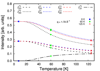
Figure 4: Scattering intensities $I^{\mathrm{A}}_{20}$ and $I^{\mathrm{A}}_{30}$, with (A = Ca, Sr, Pb), of the ground state transitions as a function of the temperature. The blue squares, the green circles and red triangles correspond to the values of the intensities given in TAB. 2.

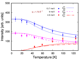
Figure 5: Scattering intensities for the compound Pb₃Cu₃(PO₄)₄ as a function of the temperature, along with experimental results from Ref. Matsuda et al. (2005). The solid and dashed lines show the calculated intensities for the Heisenberg model and Hamiltonian (5), respectively.

III.4 Energy of the magnetic transitions

Denoting the energies of transitions between energy levels by $E_{ij}$ we get

$$E_{20}=\tfrac{3}{2}J\left(1-c^{2}_{13}\right),\quad E_{30}=3J,\quad E_{31}=\tfrac{3}{2}J\left(1+c^{1}_{13}\right).$$ (30)

Neutron scattering experiments performed on $\mathrm{Pb_{3}Cu_{3}(PO_{4})_{4}}$ with $T\geq 60$ K Matsuda et al. (2005) shows the presence of a third peak at about $4.9$ meV, which may be related to the excited transition energy $E_{31}$. The values of $c^{1}_{13}$, $c^{2}_{13}$ and $J$, according to INS experiments Matsuda et al. (2005) performed on polycrystalline samples $\mathrm{A_{3}Cu_{3}(PO_{4})_{4}}$ (A = Ca, Sr, Pb) are shown in TAB. 1. In addition, for the compound $\mathrm{Ca_{3}Cu_{3}(PO_{4})_{4}}$ we have $c^{2}_{13}=-0.32(8)$ and $J\approx 4.741\,\mathrm{meV}$ based on INS data at $T=1.5$ K Furrer (2010); Podlesnyak et al. (2007).

Table 1: The values of the coupling constant and the quantities $c^{1}_{13}$, $c^{2}_{13}$ for $\mathrm{A_{3}Cu_{3}(PO_{4})_{4}}$ (A = Ca, Sr, Pb) obtained by taking into account the experimental data in Ref. Matsuda et al. (2005).

A	$E_{20}$	$E_{30}$	$E_{31}$	$c^{1}_{13}$	$c^{2}_{13}$	$J$	$J_{c^{2}_{13}}$	$J_{c^{1}_{13}}$
Ca	9.335	14.174	$-$	$-$	-0.317	4.725	0.058	–
Sr	9.936	15.064	$-$	$-$	-0.319	5.021	0.054	–
Pb	9.005	13.693	4.9	-0.284	-0.315	4.564	0.062	0.168

The temperature dependence of the integrated scattering intensities for each compound is shown on FIG. 4 obtained with the form factor (29). On FIG. 5 we present the scattering intensities for $\mathrm{Pb_{3}Cu_{3}(PO_{4})_{4}}$ computed with our Hamiltonian and the Heisenberg model along with the experimental data taken from Ref. Matsuda et al. (2005). Let us point out that our results are in better agreement with their experimental counterpart for $I_{20}^{\mathrm{Pb}}$ and $I_{30}^{\mathrm{Pb}}$, while for $I_{31}^{\mathrm{Pb}}$ we have a qualitative agreement. The averaged magnitudes of the scattering vector $q$ and the distance $r$ between neighboring ions are taken from Ref. Matsuda et al. (2005), $q=1.72\ \mathrm{\mathring{A}}^{-1}$ and $r=3.6\ \mathrm{\mathring{A}}$. The explicit expressions of the scattering intensities for each transition are

$$I^{\mathrm{A}}_{20}(T) \propto 0.5528Z^{-1}_{\mathrm{A}}e^{-\frac{E^{\mathrm{A}}_{0}}{k_{B}T}},$$ (31a)

$$I^{\mathrm{A}}_{30}(T) \propto 1.1057Z^{-1}_{\mathrm{A}}e^{-\frac{E^{\mathrm{A}}_{0}}{k_{B}T}},$$ (31b)

$$I^{\mathrm{Pb}}_{31}(T) \propto 1.1056Z^{-1}_{\mathrm{Pb}}e^{-\frac{E^{\mathrm{Pb}}_{1}}{k_{B}T}},$$ (31c)

where A = Ca, Sr, Pb. As $T$ vanishes the scattering intensities of first and second transitions from the ground state to the excited states are equal by about a factor of 2, see TAB. 2. For $T>20$ K a third peak sets in, but the evaluated intensity $I^{\mathrm{Pb}}_{31}$ remains smaller than the experimentally observed one Matsuda et al. (2005). In contrast to the functions $I^{\mathrm{Pb}}_{30}$ and $I^{\mathrm{Pb}}_{20}$ the intensities of the ground state transitions for A = Ca, Sr decrease slowly with temperature. The predicted peak for $\mathrm{Pb_{3}Cu_{3}(PO_{4})_{4}}$ is in concert with the experimental findings Matsuda et al. (2005). Unfortunately there are no experimental data confirming the presence of this third peak for the compounds $\mathrm{Ca_{3}Cu_{3}(PO_{4})_{4}}$ and $\mathrm{Sr_{3}Cu_{3}(PO_{4})_{4}}$ and hence the energy level $E_{1}$ could not be included in the sequence of energy spectrum. On FIG. 3 the presumed energy levels $E^{\mathrm{Ca}}_{1}$ and $E^{\mathrm{Sr}}_{1}$ are illustrated with dashed red lines. For all compounds the scattering intensities as a function of the magnitude of the scattering vector are represented in FIG. 6.

Table 2: Calculated values of integrated scattering intensities $I^{\mathrm{A}}_{n^{\prime}n}$ [arb. units] with A = Ca, Sr, Pb at temperatures 8, 60 and 125 K, depicted on FIG. 4

$T$ [K]	8	60	125
$I^{\mathrm{Ca}}_{20}$	0.276(4)	0.213(7)	0.141(2)
$I^{\mathrm{Ca}}_{30}$	0.552(8)	0.427(4)	0.282(5)
$I^{\mathrm{Sr}}_{20}$	0.276(4)	0.220(2)	0.146(1)
$I^{\mathrm{Sr}}_{30}$	0.552(8)	0.440(5)	0.292(2)
$I^{\mathrm{Pb}}_{20}$	0.276(4)	0.184(3)	0.113(4)
$I^{\mathrm{Pb}}_{30}$	0.552(8)	0.368(6)	0.226(8)
$I^{\mathrm{Pb}}_{31}$	0	0.067(3)	0.100(3)

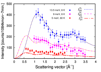
Figure 6: Calculated intensities in arbitrary units as a function of the scattering vector for Pb₃Cu₃(PO₄)₄ along with the experimental data of Ref. Matsuda et al. (2005). The dashed lines depict the intensities obtained from the Hamiltonian (5). The solid red and orange lines correspond to the Heisenberg model. $I^{\mathrm{Pb}}_{20}$ and $I^{\mathrm{Pb}}_{30}$ correspond to the ground state transitions at $T=8$ K. The intensity $I^{\mathrm{Pb}}_{31}$ stands for the excited transition at $T=60$ K. Our results show that the theoretical curves for all compounds coincide.

Figure 7: Energy level structure and the corresponding transitions of Ni₄Mo₁₂. The blue line and arrows stands for the ground state energy and the ground state excitations, respectively. The red arrow marks the excited transition and the corresponding initial level is shown in red. The dashed lines represent the centers of the two bands. All transitions are denoted with respect to the experimental data reported in Ref. Nehrkorn et al. (2010).

IV Ni₄Mo₁₂

IV.1 The Hamiltonian

The indistinguishable spin-one $\mathrm{Ni^{2+}}$ ions of the spin cluster compound $\mathrm{Ni_{4}Mo_{12}}$, are arranged on the vertices of a distorted tetrahedron FIG. 2 (a). The bonds Ni1-Ni2 and Ni3-Ni4 are slightly shorter than the other four. Distance measurements Furrer et al. (2010) report a difference of the order of $0.03\mathrm{\mathring{A}}$.

To perform an analysis of the magnetic excitations of the compound $\mathrm{Ni_{4}Mo_{12}}$ obtained by INS experiments reported in Ref. Nehrkorn et al. (2010); Furrer et al. (2010) we consider the formalism described in Section II.2. According to the symmetry of the magnetic cluster we do the imply $J_{ij}=J$ and assume that the ions Ni1-Ni2 and Ni3-Ni4 are coupled, as shown in FIG. 2 (b) by red lines, which defines these bonds as intersections of two different planes. Therefore, we have the total spin eigenstates $\lvert s_{12},s_{34},s,m\rangle$ four $\sigma$ operators for each constituent magnetic ion and two bond operators corresponding to both Ni1-Ni2 and Ni3-Ni4 spin pairs. The $\sigma$ operators $\hat{\boldsymbol{\sigma}}_{1}$ and $\hat{\boldsymbol{\sigma}}_{2}$ account for the possible changes in the superexchange processes between Ni1-Ni2 couple sharing the coefficient $a^{s_{12},m_{12}}_{12}$ of the total bond $\sigma$ operator $\hat{\boldsymbol{\sigma}}_{12}$. The operators $\hat{\boldsymbol{\sigma}}_{3}$ and $\hat{\boldsymbol{\sigma}}_{4}$ are associated with the coefficient $a^{s_{34},m_{34}}_{34}$ of the remaining $\sigma$ operator $\hat{\boldsymbol{\sigma}}_{34}$. Consequently from (5) we obtain the Hamiltonian

$$\hat{\mathcal{H}} =J\left(\hat{\boldsymbol{\sigma}}_{1}\cdot\hat{\mathbf{s}}_{2}+\hat{\boldsymbol{\sigma}}_{2}\cdot\hat{\mathbf{s}}_{1}+\hat{\boldsymbol{\sigma}}_{3}\cdot\hat{\mathbf{s}}_{4}+\hat{\boldsymbol{\sigma}}_{4}\cdot\hat{\mathbf{s}}_{3}\right)$$

$$+J\left(\hat{\boldsymbol{\sigma}}_{12}\cdot\hat{\mathbf{s}}_{34}+\hat{\boldsymbol{\sigma}}_{34}\cdot\hat{\mathbf{s}}_{12}\right).$$ (32)

With the applied effective spin-one spins the tetramer exhibits in total eighty one eigenstates without counting the quadrupolar, octupolar and other eigenfunctions related with higher symmetries. The ground state of this nanomagnet is a singlet with possible eigenstates $\{\lvert 0,0,0,0\rangle,\lvert 1,1,0,0\rangle,\lvert 2,2,0,0\rangle\}$. On the other hand, the selection rules imply that the ground state excitations must be related with singlet-triplet transitions and since the quantum numbers $s_{14}$ and $s_{23}$ cannot be simultaneously varied, we deduce that the ground state is, related to the formation of two local triplets, i.e. $s_{14}=1$ and $s_{23}=1$. The triplet eigenstates are eighteen. Those, three in total, characterized by the local quintets $s_{14}=2$ and $s_{23}=2$ are not adequate to the established selection rules and nine are identified as connected to experimental spectra.

IV.2 Energy levels

According to the selected coupling scheme we denote the eigenvalues of Hamiltonian in Eq. (IV.1) by $E^{m}_{s_{12},s_{34},s}$. The ground state is $\lvert 1,1,0,0\rangle$. Therefore, using (14) we get $a^{1,m_{12}}_{12}=a^{1,m_{34}}_{34}=1$ and taking into account (IV.1) we obtain

$$E^{0}_{1,1,0}=-8J.$$

With the eigenstates when the spins of Ni1 and Ni2 ions are coupled in a singlet, the parameter $a^{0,0}_{12}$ remains unconstrained and can be determined using INS experimental data. For the corresponding energy we get

$$E^{0}_{0,1,1}=-2Ja^{1,0}_{34}-4Ja^{0,0}_{12},\quad E^{\pm 1}_{0,1,1}=-2Ja^{1,\pm 1}_{34}-4Ja^{0,0}_{12}.$$

Analysis of Nickel spectrum yields $a^{0,0}_{12}=\{c^{1}_{12},c^{2}_{12}\}$. Thus

$$E^{\pm 1}_{0,1,1}\in\left\{-2J-4Jc^{1}_{12},-2J-4Jc^{2}_{12}\right\}.$$

Moreover, when $m_{34}=0$ we have $a^{1,0}_{34}\in\{1,-1\}$, see (16). Hence

$$E^{0}_{0,1,1}\in\left\{-2J-4Jc^{1}_{12},-2J-4Jc^{2}_{12},2J-4Jc^{1}_{12},2J-4Jc^{2}_{12}\right\}.$$

For the eigenstates corresponding to the Ni3-Ni4 singlet bond, the value of $a^{0,0}_{34}$ remains unconstrained leading to $m=m_{12}$ and according to (IV.1) we have

$$E^{0}_{1,0,1}=-2Ja^{1,0}_{12}-4Ja^{0,0}_{34},\quad E^{\pm 1}_{1,0,1}=-2Ja^{1,\pm 1}_{12}-4Ja^{0,0}_{34}.$$

We found no evidence that $a^{0,0}_{34}$ should be discrete and we set $a^{0,0}_{34}=c_{34}$. Further, with $m_{12}=0$ we have $a^{1,0}_{12}\in\{1,-1\}$. As a result we get

$$E^{0}_{1,0,1}\in\left\{-2J-4Jc_{34},2J-4Jc_{34}\right\},\quad E^{\pm 1}_{1,0,1}=-2J-4Jc_{34}.$$

For all of the remaining triplets $\lvert 1,1,1,m\rangle$, $\lvert 2,2,1,m\rangle$, $\lvert 2,1,1,m\rangle$ and $\lvert 1,2,1,m\rangle$ , where $m=0,\pm 1$, the corresponding coefficient are constrained $a^{s_{12},m_{12}}_{12}=1$ and $a^{s_{34},m_{23}}_{34}=1$. Thus, we obtain

$$E^{m}_{1,1,1}=E^{m}_{2,2,1}=E^{m}_{2,1,1}=E^{m}_{1,2,1}=-6J.$$

Furthermore, the tetramer exhibits also a singlet bond at the quintet level. The energies associated with the Ni1-Ni2 bond with singlet eigenstates $\lvert 0,2,2,m\rangle$, where $m\equiv m_{34}$ are

$$\begin{array}[]{l}E^{0}_{0,2,2}=2Ja^{2,0}_{34}-4Ja^{0,0}_{12},\quad E^{\pm 1}_{0,2,2}=2Ja^{2,\pm 1}_{34}-4Ja^{0,0}_{12},\\[5.69046pt] E^{\pm 2}_{0,2,2}=2Ja^{2,\pm 2}_{34}-4Ja^{0,0}_{12}.\end{array}$$

With $a^{2,0}_{34}\in\{1,-1\}$ and $a^{0,0}_{12}=\{c^{1}_{12},c^{2}_{12}\}$ we have

$$E^{0}_{0,2,2}\in\left\{-2J-4Jc^{1}_{12},-2J-4Jc^{2}_{12},2J-4Jc^{1}_{12},2J-4Jc^{2}_{12}\right\}.$$

When $m_{34}=\pm 1,\pm 2$, we obtain

$$\begin{array}[]{c}E^{\pm 1}_{0,2,2}\in\left\{2J-4Jc^{1}_{12},2J-4Jc^{2}_{12}\right\},\\[5.69046pt] E^{\pm 2}_{0,2,2}\in\left\{2J-4Jc^{1}_{12},2J-4Jc^{2}_{12}\right\}.\end{array}$$

Once at the quartet level the spins of third and fourth ions form a singlet, where the corresponding eigenstates are $\lvert 2,0,2,m\rangle$, then the Hamiltonian in (IV.1) yield the following energy values

$$\begin{array}[]{l}E^{0}_{2,0,2}=2Ja^{2,0}_{12}-4Ja^{0,0}_{34},\quad E^{\pm 1}_{2,0,2}=2Ja^{2,\pm 1}_{12}-4Ja^{0,0}_{34},\\[5.69046pt] E^{\pm 2}_{2,0,2}=2Ja^{2,\pm 2}_{12}-4Ja^{0,0}_{34}.\end{array}$$

Similarly, taking into account that $a^{2,0}_{12}\in\{1,-1\}$ and $a^{0,0}_{34}=c_{34}$, we obtain

$$\begin{array}[]{l}E^{0}_{2,0,2}\in\left\{-2J-4Jc_{34},2J-4Jc_{34}\right\},\\[5.69046pt] E^{\pm 1}_{2,0,2}=2J-4Jc_{34},\quad E^{\pm 2}_{2,0,2}=2J-4Jc_{34}.\end{array}$$

For the other twelve quintet states the coefficients $a^{s_{12},m_{12}}_{12}=a^{s_{34},m_{34}}_{34}=1$. Therefore,

$$E^{m}_{2,2,2}=E^{m}_{1,1,2}=E^{m}_{2,1,2}=E^{m}_{1,2,2}=-2J.$$

For the two remaining levels and the corresponding eigenstates, we obtain $a^{s_{12},m_{12}}_{12}=a^{s_{34},m_{34}}_{34}=1$. The energy sequence follows the Landé interval rule $E_{s+1}-E_{s}=2Js$, see FIG. 7. The septet level is twenty one fold degenerate. It is defined by the vectors $\lvert 2,1,3,m\rangle,\lvert 1,2,3,m\rangle,\lvert 2,2,3,m\rangle$ with $m=0,\pm 1,\pm 2,\pm 3$. All corresponding energies are equal

$$E^{m}_{2,1,3}=E^{m}_{1,2,3}=E^{m}_{2,2,3}=4J.$$

For the nonet state $\lvert 2,2,4,m\rangle$, where $m=0,\pm 1,\pm 2,\pm 3,\pm 4$ we end up with

$$E^{m}_{2,2,4}=12J.$$

The described energy level structure is illustrated on FIG. 7. In what follows we find the following notations more convenient $E_{0}=-8J,\$ $E_{1}=-2J-4Jc^{1}_{12},\$ $E_{2}=-2J-4Jc^{2}_{12},$ $E_{3}=-2J-4Jc_{34},\$ $E_{4}=-6J,\$ $E_{5}=2J-4Jc^{1}_{12}$ $E_{6}=2J-4Jc^{2}_{12},\$ $E_{7}=2J-4Jc_{34},\$ $E_{8}=-2J,$ $E_{9}=4J,\$ $E_{10}=12J$.

IV.3 Scattering Intensities

The INS selection rules are $\Delta s=0,\pm 1$, $\Delta m=0,\pm 1$ and $\Delta s_{12}=0,\pm 1$, $\Delta s_{34}=0,\pm 1$. Here the transitions $\Delta s_{12}\neq 0$ and $\Delta s_{34}\neq 0$ are not allowed simultaneously.

Using (3) we obtain $S^{\alpha\beta}(\mathbf{q},\omega_{n^{\prime}n})+S^{\beta\alpha}(\mathbf{q},\omega_{n^{\prime}n})=0,\ \forall\ n,n^{\prime}$ and $\alpha\neq\beta$. The analysis of the scattering intensities reveals the experimental magnetic excitation at $0.4$ meV Nehrkorn et al. (2010); Furrer et al. (2010) corresponding to the transition between the ground state and the singlet state $\lvert 0,1,1,\pm 1\rangle$ with

$$S^{\alpha\alpha}(\mathbf{q},\omega_{10}) =\tfrac{4}{9}[1-\cos(\mathbf{q}\cdot\mathbf{r}_{12})]p_{0},$$ (33a)

$$S^{zz}(\mathbf{q},\omega_{10}) =0,$$ (33b)

where $\alpha=x,y$. The magnetic excitation at $0.6$ meV Nehrkorn et al. (2010); Furrer et al. (2010) is associated with the eigenstate $\lvert 1,0,1,\pm 1\rangle$ and the scattering functions

$$S^{\alpha\alpha}(\mathbf{q},\omega_{30}) =\tfrac{4}{9}[1-\cos(\mathbf{q}\cdot\mathbf{r}_{34})]p_{0},$$ (34a)

$$S^{zz}(\mathbf{q},\omega_{30}) =0,$$ (34b)

where $\alpha=x,y$. The functions (33) differ from (34) due to the spatial orientations of the spin bonds with $\mathbf{r}_{12}\cdot\mathbf{r}_{34}=0$. For the same reason, we deduce that the third cold peak at $1.7$ meV Nehrkorn et al. (2010); Furrer et al. (2010) is related with the transition between the ground state and non magnetic triplet $\lvert 0,1,1,0\rangle$. For $\alpha=x,y$ the corresponding scattering functions are

$$S^{zz}(\mathbf{q},\omega_{50}) =\tfrac{4}{9}[1-\cos(\mathbf{q}\cdot\mathbf{r}_{12})]p_{0},$$

$$S^{\alpha\alpha}(\mathbf{q},\omega_{50}) =0.$$

The excited magnetic transition at around $1.2$ meV Nehrkorn et al. (2010); Furrer et al. (2010) is nicely reproduced by the scattering functions

$$S^{\alpha\alpha}(\mathbf{q},\omega_{64}) =\tfrac{2}{3}[1-\cos(\mathbf{q}\cdot\mathbf{r}_{12})]p_{4},$$

$$S^{zz}(\mathbf{q},\omega_{64}) =0,$$

where $\alpha=x,y$. The initial state is given by the triplet state $\lvert 1,1,1,\pm 1\rangle$ with two triplet bonds and the final one appears to be $\lvert 0,1,1,0\rangle$. Hence if the neutron scatters from the Ni3-Ni4 dimer, then we have $\mathbf{q}\cdot\mathbf{r}_{12}=0$ and $\mathbf{q}\cdot\mathbf{r}_{34}>0$. We remark that the orthogonality of $\mathbf{r}_{12}$ and $\mathbf{r}_{34}$ can be considered independently from the formalism presented in Section II.2. Nevertheless, with the coefficients $a^{s_{12},m_{12}}_{12}$ and $a^{s_{34},m_{34}}_{34}$ one can uniquely identify the two spin bonds and distinguish $I_{10}$ from $I_{30}$. Moreover, one can distinguish the eigenvalues of tetramer Hamiltonian corresponding to $m=0$ and $m\neq 0$, with $S^{zz}(\mathbf{q},\omega_{n^{\prime}n})=0$ and $S^{xx}(\mathbf{q},\omega_{n^{\prime}n})=0$, $S^{yy}(\mathbf{q},\omega_{n^{\prime}n})=0$, respectively. This affects directly the integrated intensities, such that choosing $\mathbf{r}_{12}=(0,0,r^{z})$ and $\mathbf{r}_{34}=(r^{x},0,0)$ from (2) yields

$$\begin{array}[]{l}\displaystyle I_{10}\propto\gamma_{10}\left[1-\frac{\sin(\mathrm{q}\mathrm{r})}{\mathrm{q}\mathrm{r}}\right]F^{2}(\mathrm{q}),\\[14.22636pt] \displaystyle I_{30}\propto\gamma_{30}\left[1-6\frac{\sin(\mathrm{q}\mathrm{r})}{5(\mathrm{q}\mathrm{r})^{3}}-3\frac{\sin(\mathrm{q}\mathrm{r})}{5\mathrm{q}\mathrm{r}}+6\frac{\cos(\mathrm{q}\mathrm{r})}{5(\mathrm{q}\mathrm{r})^{2}}\right]F^{2}(\mathrm{q}),\\[14.22636pt] \displaystyle I_{50}\propto\gamma_{50}\left[1-3\frac{\sin(\mathrm{q}\mathrm{r})}{(\mathrm{q}\mathrm{r})^{3}}+3\frac{\cos(\mathrm{q}\mathrm{r})}{(\mathrm{q}\mathrm{r})^{2}}\right]F^{2}(\mathrm{q}),\\[14.22636pt] \displaystyle I_{64}\propto\gamma_{64}\left[1-\frac{\sin(\mathrm{q}\mathrm{r})}{\mathrm{q}\mathrm{r}}\right]F^{2}(\mathrm{q}),\end{array}$$

where

$$\gamma_{10}=\tfrac{8}{9}p_{0},\ \gamma_{30}=\tfrac{20}{27}p_{0}\ \gamma_{50}=\tfrac{8}{27}p_{0},\ \gamma_{64}=\tfrac{4}{3}p_{4},$$

and $r=|\mathbf{r}_{12}|=|\mathbf{r}_{34}|$. The integrated intensities as a function of temperature are shown on FIG. 8. According to Ref. Furrer et al. (2010) the average distance between Ni-Ni ions is $\mathrm{r}=6.68\ \mathrm{\mathring{A}}$. The magnitude of the scattering vector is fixed at $\mathrm{q}=1\ \mathrm{\mathring{A}}^{-1}$ and the form factor is given by (29). The dependence of normalized intensities, $I_{n^{\prime}n}\to I_{n^{\prime}n}/\gamma_{n^{\prime}n}$, on the scattering vector is shown on FIG. 9.

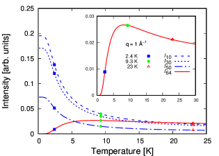
Figure 8: Intensities as a function of the absolute temperature. $I_{10}$, $I_{30}$ and $I_{50}$ correspond to the ground state transitions with energies 0.4 meV, 0.6 meV and 1.7 meV, respectively. The intensity $I_{64}$ in the inset stands for the excited transition with energy 1.15 meV. The blue squares, the green cirlces and red triangles point to the values of intensities in TAB. 3.

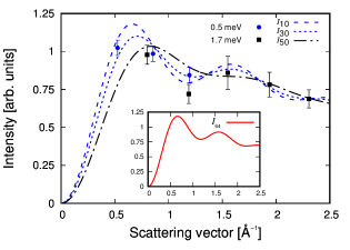
Figure 9: Normalized by $\gamma_{n^{\prime}n}$ intensities as a function of the scattering vector along with the experimental data of Ref. Furrer et al. (2010). $I_{10}$, $I_{30}$ and $I_{50}$ correspond to ground state transitions with energies 0.4 meV, 0.6 meV and 1.7 meV, respectively. The intensity $I_{64}$ stands for the excited transition with energy 1.15 meV. The inset shows the intensity $I_{64}$ that coincides with the function $I_{10}$.

Table 3: Calculated values of integrated intensities $I_{n^{\prime}n}$ [arb. units] at temperatures 2.4, 9.3 and 23 K, shown on FIG. 8 as blue squares, green circles and red trianlges, respectively.

Transitions	I	II	III	IV
$T$ [K]	$I_{10}$	$I_{30}$	$I_{50}$	$I_{64}$
2.4	0.137(6)	0.120(3)	0.051(5)	0.008(9)
9.3	0.039(8)	0.034(8)	0.014(9)	0.026(5)
23	0.019(5)	0.017(1)	0.007(3)	0.021(1)

Table 4: Values of the coupling constants and the quantities $a^{0,0}_{12}$, $a^{0,0}_{34}$ for all magnetic excitations with energies $E_{n^{\prime}n}$ obtained by taking into account the experimental data of Ref. Nehrkorn et al. (2010); Furrer et al. (2010).

Transitions	I	II	III	IV
$\mathrm{Ni_{4}Mo_{12}}$	$E_{10}$	$E_{30}$	$E_{50}$	$E_{64}$
$E_{n^{\prime}n}$[meV]	0.4	0.6	1.7	1.15
$J_{\phantom{c^{1}_{12}}}$ [meV]	0.325	0.325	0.325	0.325
$J_{c^{1}_{12}}$ [meV]	0.372	$-$	0.372	$-$
$J_{c^{2}_{12}}$ [meV]	$-$	$-$	$-$	0.353
$J_{c_{34}}$ [meV]	$-$	0.334	$-$	$-$
$c^{1}_{12}$	1.1923	$-$	1.1923	$-$
$c^{2}_{12}$	$-$	$-$	$-$	1.1153
$c_{34}$	$-$	1.0384	$-$	$-$

IV.4 Energy of the magnetic transitions

The energy transition $E_{ij}$ between $i$th and $j$th levels, corresponding to the calculated scattering intensities are

$$E_{10} =6J-4Jc^{1}_{12},\qquad E_{30}=6J-4Jc_{34},$$

$$E_{50} =10J-4Jc^{1}_{12},\qquad E_{64}=8J-4Jc^{2}_{12}.$$

From the last equations we can take advantage of one more constraint to determine $J$, $E_{50}-E_{10}=4J$. According to the experimental data Nehrkorn et al. (2010); Furrer et al. (2010) the ground state magnetic excitations are grouped in two relatively broadened peaks. The first peak is centred at about 0.5 meV and the second one at 1.7 meV. Furthermore, the first peak is composed of two subbands with energies $E_{10}=0.4$ meV and $E_{30}=0.6$ meV. The width of the second peak can be explained by the presence of an energy band, where the transition energies are restricted in the region 1.6 meV to 1.8 meV. Therefore, setting $E_{50}=1.7$ meV we obtain $E_{50}-E_{10}=1.3$ meV and $J=0.325$ meV. The computed energy transitions are depicted on FIG. 7. The centers of both energy bands referring to the value $c^{2}_{12}=1.1153$ are shown by dashed lines. The energies of all transitions and the corresponding parameters are given in TAB. 4.

V Conclusion

We propose a formalism that introduces a systematic approach for exploring the physical properties of molecular magnets. The underlying concept lies on the hypothesis that due the cluster symmetry, as well as its shape, size and the chemical structure that surrounds the magnetic ions, the exchange pathway between two particular metal ions is not unique leading to a variation of the relevant exchange energy.

To check the validity of this hypothesis we construct Hamiltonian (5) that accounts for discrete coupling parameters derived via the relations (6), (9) and (12) that allows one to distinguish spin coupling mechanisms among equivalent magnetic ions.

We apply this formalism to explore the magnetic excitations of the compounds $\mathrm{A_{3}Cu_{3}(PO_{4})_{4}}$ with (A = Ca, Sr, Pb) and $\mathrm{Ni_{4}Mo_{12}}$ obtaining results consistent with INS experiments Matsuda et al. (2005); Podlesnyak et al. (2007) and Nehrkorn et al. (2010); Furrer et al. (2010), respectively. We deduce that the ground state energy of the trimers $\mathrm{A_{3}Cu_{3}(PO_{4})_{4}}$ (A = Ca, Sr, Pb) is associated with the Cu1-Cu3 triplet bond. We obtained a thin energy band composed of two very close energy levels corresponding to the Cu1-Cu3 singlet (see e.g. FIG 3). The neutron energy loss associated with the first and the excited spin excitations is due to the transitions from triplet to singlet Cu1-Cu3 state. The second ground state excitation is the result of doublet-quartet transitions. Further, the discrete parameter $a^{0,0}_{13}\in\{c^{1}_{13},c^{2}_{13}\}$, with $|c^{i}_{13}|<1$ for $i=1,2$, shows that in the doublet level characterized by eigenstate $\lvert 0,\tfrac{1}{2},\pm\tfrac{1}{2}\rangle$ the field along all bridges between edge ions have less strength and the exchange could not be maintained. Thus, according to our calculations the next-nearest neighbor coupling $J_{13}\in\{J_{c^{1}_{13}},J_{c^{2}_{13}}\}$ is negligible, see TAB. 1. The value $|c^{1}_{13}-c^{2}_{13}|=0.031$ signals for the small variations of the next-nearest neighbor exchange coupling which therefore explains the sharpness of the experimentally observed peaks Matsuda et al. (2005); Podlesnyak et al. (2007).

Studying the INS spectra of the compound $\mathrm{Ni_{4}Mo_{12}}$ with the proposed in Sec. II.2 approach we were able to derive a detailed picture for the neutron scattering intensities FIGs. 8 and 9. Hamiltonian (IV.1) leads to energy spectrum with two energy bands, shown in FIG. 7. These bands are related to the fact that the tetramer cluster exhibits two distinguishable with respect to the coefficients $a^{s_{12},m_{12}}_{12}$ and $a^{s_{34},m_{34}}_{34}$ bonds. We ascribe this feature to the difference in the chemical environment around Ni1-Ni2 and Ni3-Ni4 couples. This allowed a unique identification of the magnetic excitations. Thereby, the obtained energy bands explain the width of second ground state peaks centred at 1.7 meV and the splitting of the first one centred at 0.5 meV. The splitting was found to be the consequence of the different spatial orientation of the Ni1-Ni2 and Ni3-Ni4 bonds (see e.g. FIG. 2). In particular, for $s_{12}=0$, $s_{34}=0$ and $i=1,2$ we get $|c^{i}_{12}|>1$ and $|c_{34}|>1$, respectively. Besides, according to (20) we have $J<J_{c^{i}_{12}}$ and $J<J_{c_{34}}$, see TAB. 4. These inequalities signals that the strength of the exchange is amplified. Furthermore, the inequality $J_{c_{34}}<J_{c^{i}_{12}}$ indicates that most probably the field has less strength along Ni3-Ni4 bond than the Ni1-Ni2 one.

In the present study we confined ourselves to the explanation of experimental INS spectra of some representative trimers and tetramers. We would like to mention that the method can be applied to other magnetic properties, such as the magnetization and the susceptibility. We would like to anticipate that preliminary results are encouraging and will be the subject of a separate paper.