On the use of the main sequence knee (saddle) to measure globular cluster ages

Abstract

In this paper we review the operational definition of the so-called main sequence knee (MS-knee), a feature in the color-magnitude diagram (CMD) occurring at the low-mass end of the MS. The magnitude of this feature is predicted to be independent of age at fixed chemical composition. For this reason, its difference in magnitude with respect to the MS turn-off (MS-TO) point has been suggested as a possible diagnostic to estimate absolute globular cluster (GC) ages.

We first demonstrate that the operational definition of the MS-knee currently adopted in the literature refers to the inflection point of the MS (that we here more appropriately named MS-saddle), a feature that is well distinct from the knee and that cannot be used as its proxy. The MS-knee is only visible in near-infrared CMDs, while the MS-saddle can be also detected in optical-NIR CMDs.

By using different sets of isochrones we then demonstrate that the absolute magnitude of the MS-knee varies by a few tenths of a dex from one model to another, thus showing that at the moment stellar models may not capture the full systematic error in the method.

We also demonstrate that while the absolute magnitude of the MS-saddle is almost coincident in different models, it has a systematic dependence on the adopted color combinations which is not predicted by stellar models.

Hence, it cannot be used as a reliable reference for absolute age determination. Moreover, when statistical and systematic uncertainties are properly taken into account, the difference in magnitude between the MS-TO and the MS-saddle does not provide absolute ages with better accuracy than other methods like the MS-fitting.

1 Introduction

Globular clusters (GCs) are among the oldest stellar aggregates in the Universe and are therefore pristine fossils of the very early epoch of galaxy formation. A detailed study of their ages is useful for several reasons: relative ages help us to understand the formation and the assembly chronology of the different components (halo, disk, bulge) of our Galaxy (Rosenberg et al., 1999; Zoccali et al., 2003, Marín-Franch et al., 2009); absolute ages set a lower limit to the age of the Universe (Buonanno et al., 1998, Stetson et al., 1999, Gratton et al. (2003)) and provide robust constraints to the physics adopted in stellar evolutionary models (Salaris & Weiss, 1998; Cassisi et al., 1999; VandenBerg et al., 2008; Dotter et al., 2008). Several methods have been used so far to estimate the relative and absolute ages of these systems, mainly based on the analysis of their optical CMDs.

Relative ages can be derived by using “differential” parameters, built from the magnitude or the color of the main sequence turn-off point (MS-TO, which systematically varies with time) and the magnitude or the color of a “reference” feature in the CMD that is independent of the cluster age. Examples are: (1) the horizontal parameter, defined as the difference in color between the MS-TO and the red giant branch (RGB) at 2.5 magnitudes above the MS-TO level (see Sarajedini & Demarque, 1990; Sandage, 1990; Vandenberg et al., 1990); (2) the vertical parameter, based on the difference in magnitude between the horizontal branch (HB), typically measured at the RR Lyrae instability strip, and the MS-TO (Iben & Renzini, 1984; Buonanno et al., 1998; Rosenberg et al., 1999; Stetson et al., 1999; De Angeli et al., 2005). Of course differential parameters have the advantage of being independent of distance and reddening.

Cluster absolute ages are generally estimated by measuring the luminosity of the MS-TO point in the CMD, or by applying the isochrone fitting method. The latter has been recently used by Saracino et al. (2016) and Correnti et al. (2016), to determine sub-Gyr absolute ages using a chi-squared minimization and a maximum-likelihood technique, respectively. Absolute ages can also be derived from the direct comparison of the differential parameters with the corresponding theoretical predictions. In these cases, various sets of theoretical models (e.g., Pietrinferni et al. (2004); Salaris & Weiss, 2002; Dotter et al., 2010; VandenBerg et al., 2013) need to be considered in order to investigate the effects of different assumptions in the models. This effect becomes quite important when low-mass stars are considered in the analysis. More in general, the reliability of the absolute ages derived from classical methods almost totally depends on the accuracy of the adopted distances and chemical abundances.

In the recent years, advanced instruments and techniques, such as adaptive optics systems mounted on 8-10 m class telescopes, and high resolution cameras on board the Hubble Space Telescope (HST), make also near-infrared (NIR) observations very promising in the estimate of GC ages. In fact, deep NIR photometry revealed the existence of a well-defined knee at the lower end of the MS, approximately three magnitudes below the MS-TO (see, e.g., the cases of $\omega$ Centauri, Pulone et al., 1998; M4, Pulone et al., 1998; Milone et al., 2014; NGC 3201, Bono et al., 2010; NGC 2808, Milone et al., 2012; Massari et al., 2016; 47 Tucanae, Kalirai et al., 2012; M71, Di Cecco et al., 2015; M15, Monelli et al., 2015).

The MS-knee arises from a redistribution of the emerging stellar flux due to an opacity change, mainly caused by the collision-induced absorptions of molecular hydrogen in the surface of cool dwarfs (Linsky, 1969; Saumon et al., 1994 and references therein), which moves low-mass MS stars towards bluer colors. Since its magnitude is predicted to be independent of cluster age at fixed chemical composition, the MS-knee provides a potential anchor (alternative to the HB luminosity) at which the MS-TO magnitude can be referred to define a new vertical method for the age determination, independent of GC distance and reddening. With respect to the traditional vertical method referred to the HB level, it has the drawback of requiring the detection of a much fainter feature in the CMD (fainter by $\sim 7$ magnitudes), but i) it is much more populated because the stellar luminosity function increases towards lower masses and ii) it should be less affected by model uncertainties, such as the treatment of convection (Saumon & Marley, 2008). For these reasons Bono et al. (2010) proposed a new parameter (hereafter $\Delta^{\rm knee}_{\rm TO}$) to measure relative and absolute GC ages from the magnitude difference between the MS-TO and the MS-knee levels. The method has been already tested on a few clusters (as NGC 2808, Massari et al., 2016; M71, Di Cecco et al., 2015 and M15, Monelli et al., 2015), with the conclusion that it can provide absolute age estimates at sub-Gyr accuracy, a factor of two better than what can be obtained with classical methods. Relative age studies using the $\Delta^{\rm knee}_{\rm TO}$ method have not been performed yet.

This paper provides an in-depth analysis of both the operational definition of the MS-knee and the potential use of this feature to estimate absolute GC ages. Our study is based on both widely used stellar models and photometric observations of the low-mass MS in two well known GCs.

In Section 2 we summarize the diagnostic tools used to perform the analysis. In Section 3 we review the operational definition of the MS-knee adopted in the literature, suggesting a more appropriate nomenclature: we name MS-knee the point in a NIR CMD where the MS bends to the blue, while we name MS-saddle the point where the MS changes curvature. In Section 4 we describe the procedure followed in order to measure the MS-saddle in the two GCs 47 Tucanae and NGC 6624, and in Section 5 we discuss their derived ages and uncertainties. In Section 6 we draw our conclusion.

2 Diagnostic tools

Our analysis of the low-mass MS and its most important features has been performed by using the following theoretical and observational tools:

• Stellar models - We considered three different sets of $\alpha$-enhanced stellar models, namely A Bag of Stellar Tracks and Isochrones (BaSTI; Pietrinferni et al., 2004), the Dartmouth Stellar Evolutionary Database (DSED; Dotter et al., 2007) and the Victoria-Regina isochrones (VR; VandenBerg et al., 2014). The BaSTI NIR colors and magnitudes are on the Johnson-Cousins-Glass photometric system, while the DSED and VR isochrones are on the 2MASS photometric system. Hence, for a coherent comparison, we adopted the 2MASS photometric system as reference and we converted the BaSTI NIR colors first on the Bessell & Brett (1988) system and then, by using the transformations of Carpenter (2001), into the 2MASS photometric system (Cutri et al., 2003).
  BaSTI, DSED and VR isochrones assume different solar mixture abundances, which are based on Grevesse & Noels (1993), Grevesse & Sauval (1998) and Asplund et al. (2009), respectively. To obtain the same chemical content, in terms of [M/H], for the three sets of isochrones, we adopt the same $\alpha$-element abundance ([$\alpha$/Fe] = +0.4) but we are forced to adopt slightly different [Fe/H] (see Table 1 for a detailed comparison of the adopted isochrones). We note that this is an approximation as other metals (e.g. differences in the C+N+O abundance) can play a role. However, we stress that small changes to the assumed metal abundances are expected to have much smaller effects on isochrones along the MS than other factors, such as the color-temperature transformations to the observed diagrams (see below).

• Observed GCs - Deep and accurate photometry of the low-mass MS of two GCs, namely 47 Tucanae and NGC 6624, having similar chemical composition ([Fe/H]=-0.69 and -0.60 respectively; see Correnti et al. (2016) and reference therein and Saracino et al. (2016) and reference therein), has been used as an empirical test bench for our analysis. For 47 Tucanae we used the catalog presented in Kalirai et al. (2012), based on images acquired using the infrared channel of the Wide Field Camera 3 (WFC3) on board the HST in the $F110W$ and $F160W$ filters (GO-11677 PI: Richer). The resulting ($F110W,F110W-F160W$) CMD is shown in the left panel of Figure 1. It exhibits very well defined evolutionary sequences, from the base of the RGB to the low-mass end of the MS, reaching $\sim$ 3 magnitudes below the MS-knee. The photometric precision is of the order of a few thousandths of a magnitude over the luminosity range sampled: $\approx$ 0.002 mag at the MS-TO level, $\approx$ 0.005 at the MS-knee. Since the Kalirai et al. (2012) catalog samples only the external regions of the cluster, no optical data of comparable depth are available. In the case of NGC 6624, we have used the catalog described in Saracino et al. (2016). It has been obtained by using $J$ and $K_{s}$ images of the central regions of the cluster acquired with the multi-conjugate adaptive optics system GeMS at the Gemini South Telescope in Chile, as part of the proposal GS-2013-Q-23 (PI: D. Geisler). A detailed description of the observations and the data-reduction procedure is reported in Section 2 of Saracino et al. (2016). The ($K_{s},J-K_{s}$) CMD of NGC 6624 is presented in the right panel of Figure 1. It spans a range of more than 8 magnitudes, from the HB level down to $K_{s}\approx 21.5$. In this case, the photometric errors are of $\approx$ 0.005 mag at the MS-TO level and $\approx$ 0.035 mag at the MS-knee. We have also combined the GEMINI catalog of Saracino et al. (2016) with the optical HST-Advanced Camera for Survey (ACS) catalog of Sarajedini et al. (2007), providing $V$ and $I$ data for the stars in common.

• CMDs - We investigated the low-mass MS properties in various CMDs, namely the ($F110W,F110W-F160W$) CMD, where theoretical isochrones are compared with HST NIR photometry of 47 Tucanae, and in the ($K_{s},J-K_{s}$), ($K_{s},I-K_{s}$), and ($K_{s},V-K_{s}$) CMDs, where theoretical isochrones are compared with ultra-deep NIR (ground-based) and optical (HST) photometry of NGC 6624. Note that the hybrid optical-NIR CMDs are the most used in the literature to detect the MS-saddle (see Bono et al., 2010, Monelli et al., 2015, Di Cecco et al., 2015 and Massari et al., 2016).

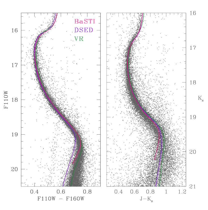
Figure 2: Left panel – ($F110W,F110W-F160W$) CMD of 47 Tucanae, with BaSTI, DSED and VR isochrones superimposed in magenta, violet and green respectively. Right panel – ($K_{s},J-K_{s}$) CMD of NGC 6624 with the adopted isochrones overimposed. The color code is shown in the legend.

In Figure 2 we show a comparison of the ($F110W,F110W-F160W$) CMD for 47 Tucanae and of the ($K_{s},J-K_{s}$) CMD for NGC 6624 with theoretical models. We adopted the following parameter values from the literature: $t=11.5$ Gyr, $E(B-V)=0.04$, $(m-M)_{0}=13.31$ for 47 Tucanae (Correnti et al., 2016) and $t=12.0$ Gyr, $E(B-V)=0.28$, $(m-M)_{0}=14.49$ for NGC 6624 (Saracino et al., 2016). The color code is the same in both panels, where the magenta, violet and green lines refer to the adopted BaSTI, DSED and VR isochrones, respectively. As can be seen, the general agreement in MS between our data and the theoretical models is quite satisfactory. Few exceptions: in the ($F110W,F110W-F160W$) CMD the DSED isochrone turns out to be bluer than the other two models at magnitudes fainter than $F110W=19$, while in the ($K_{s},J-K_{s}$) CMD a similar behavior is observed for the BaSTI isochrone at $K_{s}>19.5$, but with a smaller discrepancy.

3 A knee or a saddle?

As shown in Figure 3, in a pure NIR ($K_{s},J-K_{s}$) filter combination, the lowest portion of the MS bends to the blue and creates a well defined knee. Consistently, the MS-knee (marked with a red circle in the figure) corresponds to the reddest point of the MS at magnitudes fainter than the MS-TO. However, the MS-knee has been originally defined as the point of minimum curvature along the low-mass end of the MS ridge line (see Bono et al., 2010). This is an inflection point (that we name MS-saddle), where the MS ridge line changes its curvature from convex to concave. While it is related to the presence of the knee, it is certainly not coincident with it. This is clearly illustrated in Figure 3, where the location of the two features is marked along a 12 Gyr old VR isochrone: the MS-saddle (blue square, characterized by $\approx 0.65\;M_{\odot}$ stellar mass) is more than 0.7 mag brighter than the MS-knee (red circle, characterized by $\approx 0.55\;M_{\odot}$ stellar mass).

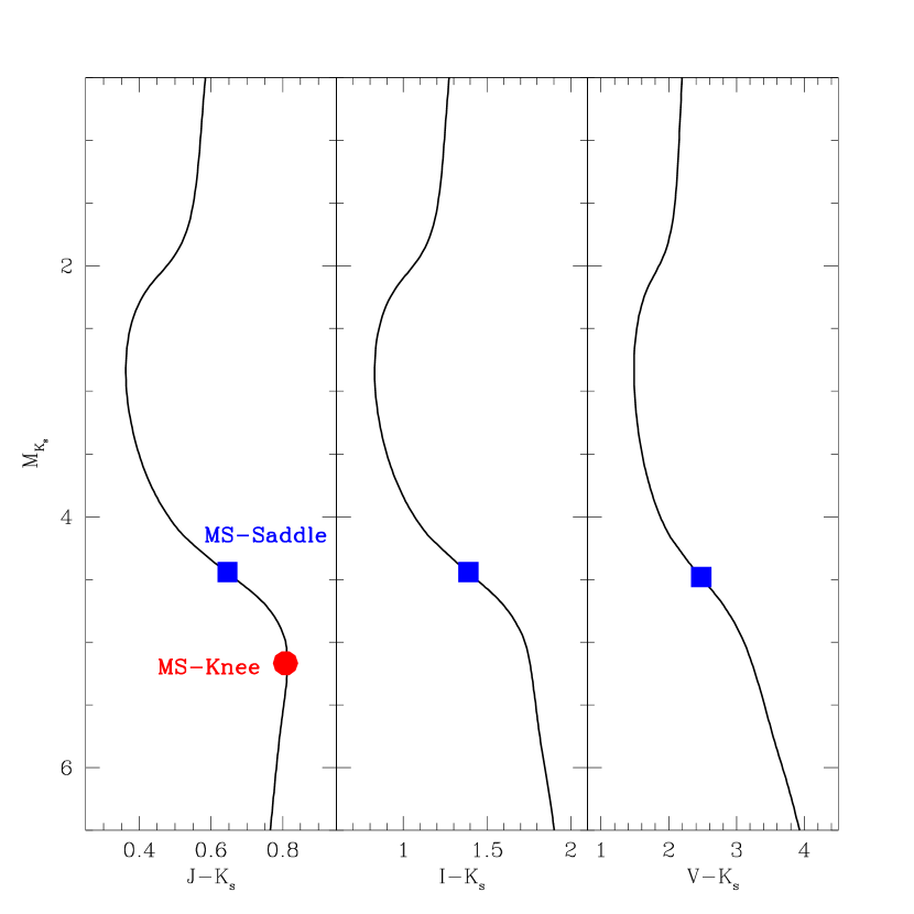
Figure 4: Location of the MS-knee (red circle) and MS-saddle (blue square) marked along the same isochrone plotted in Figure 3, but here shown in CMDs with three different colors: from left to right, ($K_{s},J-K_{s}$), ($K_{s},I-K_{s}$), and ($K_{s},V-K_{s}$). The MS-knee only occurs in the pure NIR-CMD. The MS-saddle, instead, can be defined in all the considered diagrams.

However, the MS-saddle can be of interest. In fact, as shown in Figure 4, while the MS-knee only occurs in NIR CMD (red circle in the left panel) and it is not definable in hybrid optical-NIR CMDs (middle and right panels), the MS-saddle (blue squares) can be measured in all the diagrams. Hence, a detailed comparison between the two features is worth investigating, in particular to assess whether the MS-saddle can be considered as a proxy of the MS-knee and it can be used for measuring cluster ages.

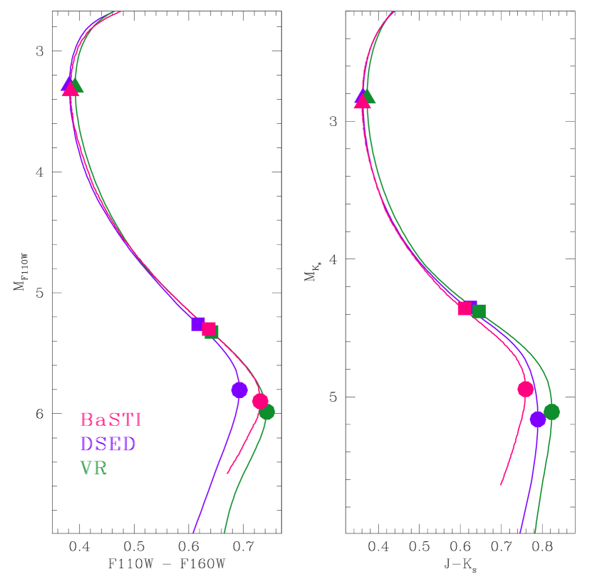
Figure 5: Location of the MS-TO (triangles), MS-knee (circles) and MS-saddle (squares) marked along 12 Gyr old isochrones from three different sets of theoretical models: BaSTI (magenta), DSED (violet) and VR (green) in the ($K_{s},J-K_{s}$, left panel) and ($F110W,F110W-F160W$, right panel) filter combinations. The three models predict different locations of the MS-knee, while they agree on the color-magnitude position of the MS-saddle. This clearly illustrates that the two features are different.

To this end, in Figure 5 we compare the BaSTI, DSED and VR isochrones at a fixed age of $t=12$ Gyr in the ($K_{s},J-K_{s}$) CMD (left panel) and in the ($F110W,F110W-F160W$) CMD (right panel). Triangles, squares and circles mark the MS-TO, the MS-saddle and the MS-knee, respectively, along each isochrone. As can be seen, the three models predict the same location in the CMD for the MS-TO and the MS-saddle, but significantly different positions of the MS-knee. As a consequence, for the same age and metallicity, the three isochrones predict values of $\Delta^{\rm knee}_{\rm TO}$ differing by 0.26 magnitudes in the $K_{s}$ filter, ranging from 2.08 to 2.36. A similar difference has been also measured in the $F110W$ filter, indicating that such a discrepancy among different models does not depend on the used NIR filters and filter combinations.

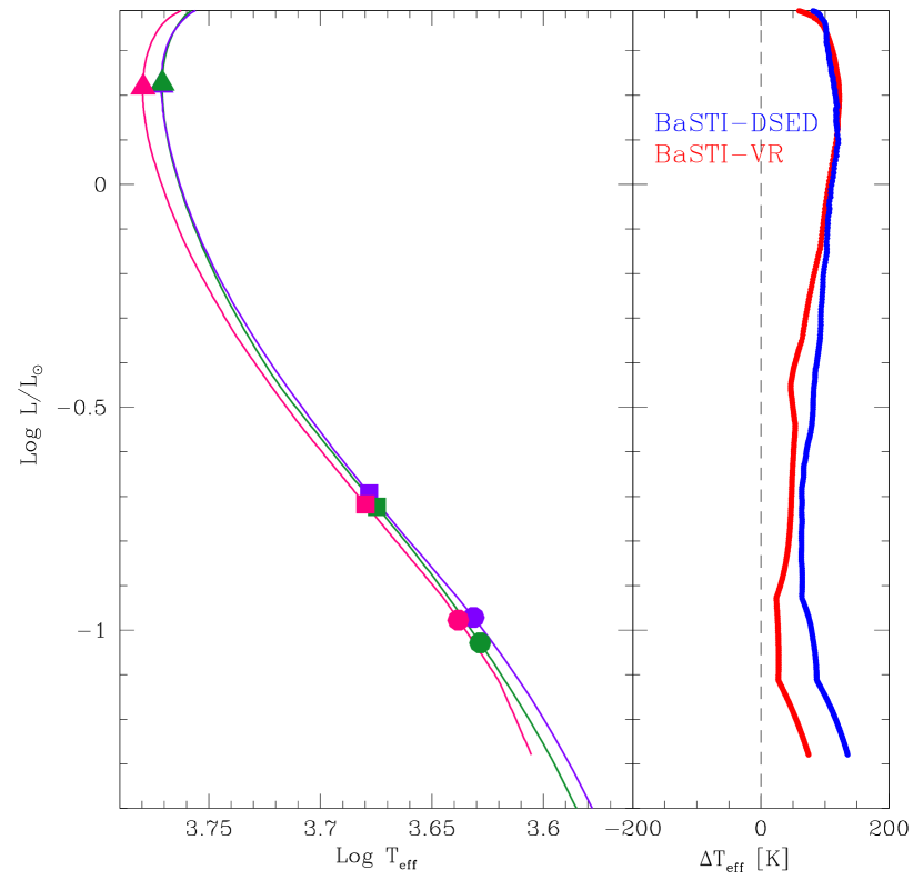
Figure 6: Left panel: Color and magnitude of the MS-saddle (squares) and MS-knee (circles) points shown in Figure 4 are translated here in temperature and luminosity, respectively. Right panel: At fixed luminosity, the $\Delta T_{eff}$ between two pairs of models (BaSTI-DSED) and (BaSTI-VR) is presented in blue and red, respectively.

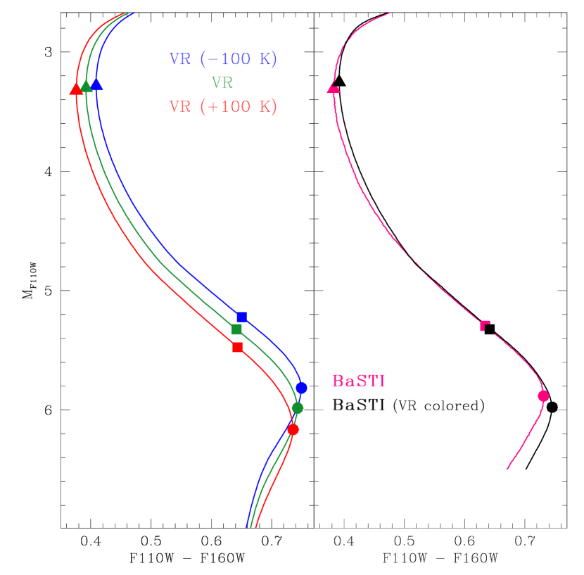
Figure 7: Left panel: A VR isochrone is adjusted to hotter (red line) and cooler (blue line) temperatures by 100 K with respect to the normal one (green line) and then transformed to the observed ($F110W,F110W-F160W$) plane. Right panel: In the same filter combination, a BaSTI isochrone colored using its usual BCs is shown in magenta, compared to the same isochrone colored using the Casagrande & VandenBerg (2014) BCs (in black). Triangles, squared and circles indicate the MS-TO, MS-saddle and MS-knee, respectively, in both panels.

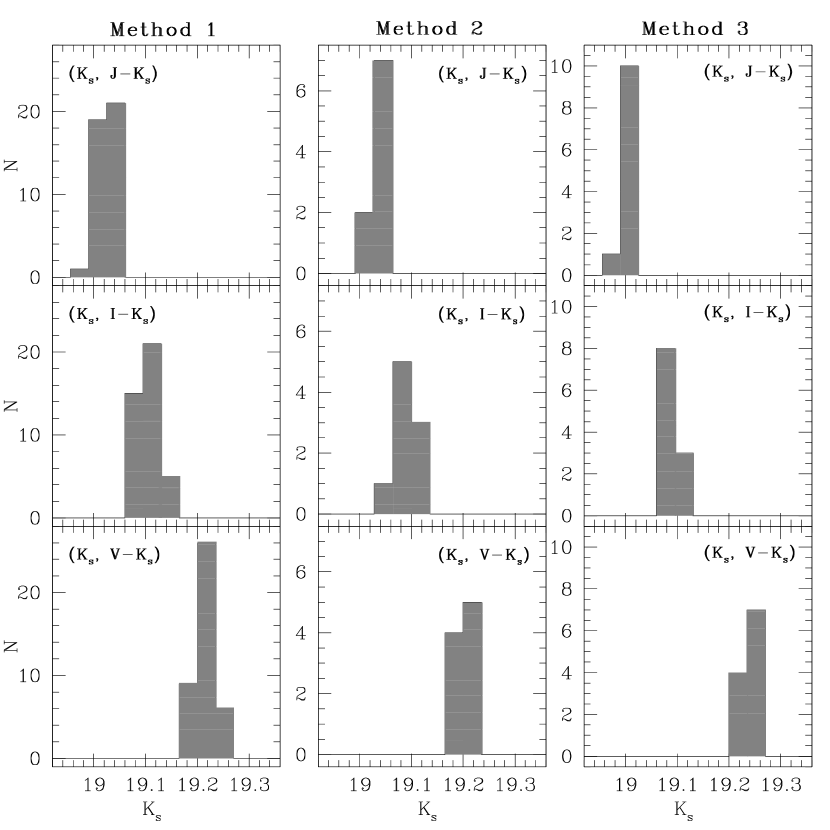
Figure 9: Histograms of the MS-saddle $K$-band magnitude measured in the ($K_{s},J-K_{s}$), ($K_{s},I-K_{s}$), and ($K_{s},V-K_{s}$) CMDs (upper, middle, and bottom rows, respectively), for NGC 6624. Multiple measures of this value have been obtained in each case because the MS MRL has been determined with different methods (see Sect. 3.1): Method 1 - static bins (left column, providing 41 MRLs and 41 measures of the MS-saddle magnitude), Method 2 - dynamic bins (central column, 9 measures), and Method 3 - Polynomial fit (right column, 11 measures).

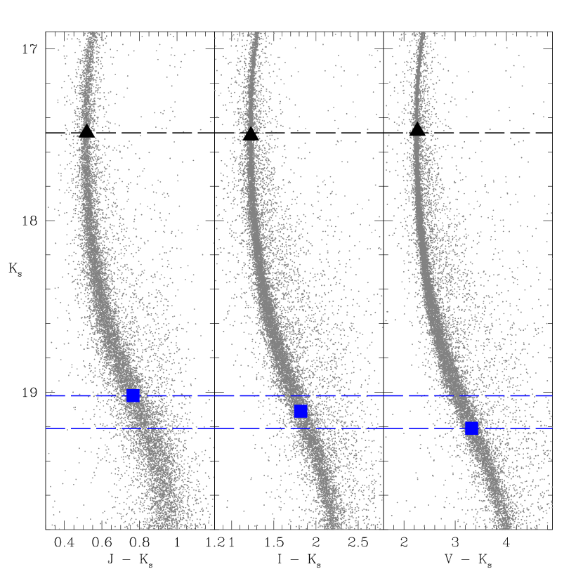
Figure 10: Location of the MS-TO (black triangle) and MS-saddle (blue square) in the three CMDs available for NGC 6624. The horizontal black dashed line marks the MS-TO level, the horizontal dashed blue lines the two extreme values of the MS-saddle, which differ by 0.2 mag.

In Figure 6 (left panel), the color and the magnitude of the MS-knee points shown in Figure 5 are translated in effective temperature ($T_{eff}$) and luminosity ($L$), respectively. As can be seen, they are located in a region where stellar models differ in shape also in the Hertzsprung - Russell (HR) diagram.
To quantify such differences, we selected a reference model (BaSTI) and we measured the difference in effective temperature ($\Delta T_{eff}$) at fixed luminosity between the two model pairs (BaSTI - DSED) and (BaSTI - VR), respectively. The results are shown in the right panel of Figure 6, where differences up to $\Delta T_{eff}$ $\approx$ 100 K are observed both at the MS-TO and MS-knee levels.
The $\Delta T_{eff}$ at the MS-knee is mostly due to the uncertain choice of the stellar model boundary conditions, as discussed e.g. by Chen et al. (2014). One can clearly see in their Figures 5, 6, 9 and 10, that a small change of the boundary conditions affects the position of theoretical GCs isochrones in the ($L-T_{eff}$) diagram at the typical bolometric luminosities of the MS-knee. The difference observed at the MS-TO can be attributed to differences in the absolute C+N+O abundance and adopted physics among the three models.
To quantify the impact that a variation in temperature has on the position of the MS-TO and the MS-knee points, we used a VR isochrone as reference. We applied shits in temperature of $\pm$ 100 K and then we transformed it into the observed diagram by using the Casagrande & VandenBerg (2014) transformations. The results are presented in the left panel of Figure 7, in the ($F110W,F110W-F160W$) filter combination. A $\Delta T_{eff}$ = $\pm$ 100 K translates into a difference of $\pm$ 0.02 mag in the MS-TO position and a difference of $\pm$ 0.15 mag in the MS-knee position. However, these values are able to explain only half of the observed discrepancies at both levels.
In this context, it is worth to note that BaSTI, DSED and VR isochrones are based on different model atmospheres (BaSTI - Castelli & Kurucz (1994); DSED - PHOENIX (Husser et al., 2013) and VR - MARCS (Gustafsson et al., 2008)), thus they use different bolometric corrections (BCs) and color-temperature transformations (see e.g. Salaris et al., 2007; Brasseur et al., 2010; Cohen et al., 2015).
In Figure 7, right panel, we show the effect of adopting different BCs. In particular, we compare a BaSTI isochrone with the corresponding one after applying BCs from Casagrande & VandenBerg (2014). As can be seen, also BCs play a role in shaping the low-mass MS at NIR wavelengths. In fact, they account for differences of about 0.1 mag, 0.02 mag and 0.04 mag at the MS-knee, MS-saddle and MS-TO, respectively, thus becoming an important source of uncertainty.
The interplay between variations in $T_{eff}$ among models and adopted BCs produce final discrepancies of more than 0.2 mag on the MS-knee position, of about 0.05 mag and 0.04 mag on the MS-saddle and MS-TO positions, respectively, which are fully consistent with what observed both in Figures 5 and 6.

Major progress in model atmosphere calculations for low-mass and very low-mass stellar models (that provide both BCs and model boundary conditions) is needed for firmer theoretical predictions about the MS-knee.

Hence, at the moment, because of the large uncertainties currently affecting the theoretical models, the MS-knee can be safely adopted only for relative age studies where a comparison between different stellar models is not necessary.

The location of the MS-saddle appears to be much more stable (with magnitude variations among different models smaller than 0.05 mag in $K_{s}$ and in the corresponding bolometric luminosity, see Figures 5 and 6), demonstrating that the MS-saddle is not very sensitive to the morphology and the location of the knee. Hence the first result of this investigation is that the MS-saddle cannot be used as a proxy for the MS-knee. However its reduced model-dependence and its potential measurability also in combined optical-NIR CMDs call for a thorough investigation of its reliability and stability as a reference feature to estimate cluster ages.

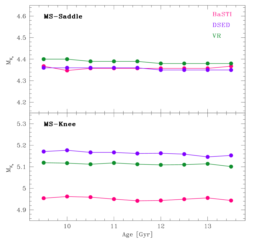
Figure 8: Upper panel– Dependence of the MS-saddle $K_{s}$-band magnitude on cluster age for the three different sets of adopted isochrones (BaSTI, DSED and VR in magenta, violet and green, respectively). Ages vary from 9.5 to 13.5 Gyr in steps of 0.5 Gyr. At fixed chemical composition, the MS-saddle $K_{s}$-band magnitude is independent of age and shows small dependence on the adopted model. Lower panel – The same as in the upper panel, but for the MS-knee. In this case, different models predict significantly different values of the $K_{s}$-band magnitude of the MS-saddle (see Figure 5 for further details).

Of course, the first requisite is that, for fixed chemical composition, the magnitude of the MS-saddle is independent of the cluster age. This is indeed confirmed by all the stellar models considered above. The predicted $K_{s}$-band magnitude of the MS-saddle (and, for comparison, of the MS-knee) for stellar populations with ages ranging from 9.5 Gyr to 13.5 Gyr is shown in Figure 8 for the three families of adopted stellar models. The constancy of the MS-saddle magnitude with varying the isochrone age indicates that, in principle, it can be used as an anchor to which the MS-TO can be referred and used to measure both relative and absolute ages. However, since it is a geometric point, dependent on the morphology of the MS ridge line, it can be a somewhat fragile feature both from an observational and a theoretical point of view, requiring detailed investigation.

4 Measuring the MS-saddle

The first step to locate the MS-saddle in an observed CMD of a GC is to determine the cluster mean-ridge line (MRL).

The catalog adopted for 47 Tucanae was already cleaned from spurious objects (Kalirai et al., 2012). In the case of NGC 6624 CMDs, a selection in the stellar sharpness parameter (defined as in Stetson et al., 1989) was applied. We divided the sample of stars in our catalog in 0.5 magnitude-wide bins and for each bin we computed the median sharpness value and its standard deviation ($\sigma$). Only stars with sharpness parameter lying within 6$\sigma$ from the median were flagged as “well-measured”.

The “clean” photometric catalogs were used to determine the MRL in each of the four considered CMDs, namely ($F110W,F110W-F160W$) for 47 Tucanae and ($K_{s},J-K_{s}$), ($K_{s},I-K_{s}$) and ($K_{s},V-K_{s}$) for NGC 6624.

This was done by using three different methods in order to evaluate the impact of slightly different MRLs on the location of the MS-saddle and to derive the precision achievable in measuring this feature.

Method 1: Static bins - we considered different magnitude bins (in $F110W$ for 47 Tucanae and $K_{s}$ for NGC 6624) and we computed the mean color of all the stars falling in each bin, by applying an iterative 2$\sigma$-rejection procedure. We allowed the bin size to vary from 0.10 mag (lower limit, necessary to have a reasonable number of stars per bin) to 0.50 mag (upper limit, imposed to keep an accurate sampling of the fiducial line), in steps of 0.01 mag. At the end of the procedure, for each of the four filter combinations, we had 41 (differently sampled) MRLs, which have been re-sampled with a 0.01 mag-stepped cubic spline.

Method 2: Dynamic bins - This method uses bins of constant size in magnitudes partially overlapping. This means that, at any fixed bin size, the MRLs derived from dynamic bins are more densely sampled (at higher resolution) than those obtained from static bins. In this case we modified the bin size from 0.10 mag to 0.50 mag in steps of 0.05 mag, obtaining a sampling of 0.05 mag for each MRL. The resulting 9 MRLs per each filter combination have also been re-sampled with a cubic spline of 0.01 mag steps.

Method 3: Polynomial fit - This method directly performs a polynomial fit to the observed sequences in the CMD. The degree of the polynomial has been chosen as a compromise between having an adequate ability to reproduce the shape of the MS in the CMD and the need of limiting the number of coefficients. We thus produced 11 different MRLs per CMD by varying the degree of the polynomial from 5 to 15, in step of 1.

The visual inspection of the MRLs derived with the three methods for each cluster in each color combination shows that they are all similar and they provide equivalently good representations of the cluster MS. However, in order to test the effect of adopting slightly different MRLs we determined the MS-TO and the MS-saddle in all the obtained MRLs, separately. In doing this we adopted the following prescriptions: i) The MS-TO has been defined as the bluest point of the MS. This is one of the classical and most used definitions and it allows an easy estimate of the error on its determination.

ii) The MS-saddle is defined as the point of minimum curvature along the MS. To measure it we used both an analytical and a geometric method.

Analytical method: we defined the MS-saddle as the point where the second derivative of the MRL is equal to zero.

Geometric method: we adopted the “circumference method” described in Massari et al. (2016). It consists in determining the circumference that connects each point of the MRL with the two adjacent/contiguous points located at $\pm$ 0.5 mag, and then adopt as MS-saddle the point corresponding to the circumference with the largest radius (minimum curvature). Following the suggestion in Massari et al., 2016, we tested the robustness of such a procedure by changing the distance in magnitude among the three points on the MRL from 0.1 mag to 0.8 mag, in steps of 0.1 mag. This provided us with 8 different estimates of the MS-saddle point for each MRL. In all cases the 8 measures nicely agree (typically within $\pm 0.03$ mag). Hence, their average value has been adopted as final “geometric” measure of the MS-saddle.

The application of different methods for determining the cluster MRL and the use of different CMDs affect the estimate of the MS-saddle magnitude as illustrated in Figure 9 for NGC 6624. The results are shown for the “geometric” measure of the MS-saddle; those obtained from the analytical method are fully consistent. According to the description above, we have derived 41, 9 and 11 MLRs from methods 1, 2 and 3, respectively, for each color. Hence, the three panels in the upper row of Figure 9 show the distribution of the 41, 9 and 11 values of the MS-saddle $K_{s}$-band magnitude determined in the ($K_{s},J-K_{s}$) CMD from the three methods. The middle and bottom rows show the analogous results obtained from the ($K_{s},I-K_{s}$) and ($K_{s},V-K_{s}$) diagrams. For a given CMD (along each row in the figure) the estimated magnitude of the MS-saddle is essentially independent of the method adopted to determine the MRL (all the measures agree within $\pm 0.04$ mag). However, for any fixed method to determine the MRL, the magnitude of the MS-saddle varies by 0.2-0.25 mag when different CMDs are considered (i.e., along each column in Figure 9). In particular, the MS-saddle $K_{s}$-band magnitude shows a systematic trend with the color, becoming increasingly fainter for color combinations that involve filters at shorter wavelengths. This is also illustrated in Figure 10, where the MS-saddle point (determined as the average of the 41 measures resulting from the “static bins” and the “geometric” methods) is marked with a blue square in each of the three available CMDs. This trend might be an indirect effect induced by the presence and the relevance of the MS-knee on the shape of the MS MRL. In fact the presence of a clear knee in the ($K_{s},J-K_{s}$) CMD (see the left panel of Figure 4) might require an “early change” in the curvature of the MRL (i.e. the inflection point must occur at relatively bright luminosity). Instead, as soon as the knee disappears becoming a “light bend” in the MRL (middle and right panels of Figure 4), the change in the MRL curvature becomes “less pronounced” (i.e. the inflection point tends to slide to fainter luminosities). At odds with the systematic drift of the MS-saddle magnitude with the color, the measures of the MS-TO stay nicely stable (within 0.02 mag) independently of the considered CMD. This is also apparent in Figure 10 (black triangles). If the CMD location of the MS-saddle significantly depends on the details of the MS MRL morphology, theoretical isochrones have to predict such a trend accordingly. If not, this might introduce some systematic in estimating age using this feature.

Since the magnitude of the MS-saddle does not depend on the method used to determine the MRL, in the following we will consider only the values obtained from Method 1 (static bins), which also provides the largest statistics (41 data points). The magnitudes of the MS-TO and MS-saddle (and their uncertainties) obtained as the average (and the standard deviation) of the 41 measurements in each of the available color combinations are listed in Table 2. For 47 Tucanae the listed magnitudes are in the $F110W$ band, while for NGC 6624 they are in the $K_{s}$ band. The last two columns of the table list the values obtained from the two methods (analytic and geometric) used to identify the MS-saddle point along the MRL. As can be seen, the results are fully consistent and in the following we will thus adopt the values obtained from the geometric approach, which has been already used in the literature.

We finally estimated the parameter $\Delta^{\rm saddle}_{\rm TO}$ from the difference between the adopted MS-saddle and MS-TO magnitudes and we derived the uncertainties by taking into account: (1) the error associated to the MS-TO determination; (2) the uncertainty related to the MS-saddle point and (3) the photometric error affecting both parameters. Photometric errors are an additional source of uncertainty in the derivation of the MS-saddle and the MS-TO positions, so they have to be taken into account. They have been computed as the average of the photometric errors (in $F110W$ and in $K_{s}$ for 47 Tucanae and NGC 6624, respectively) of all the stars falling within $\pm$ 0.1 magnitudes from the MS-TO and the MS-saddle points. In the case of 47 Tucanae, we obtained $\sigma_{F110W,\rm{MSTO}}=0.002$ mag and $\sigma_{F110W,\rm{saddle}}=0.005$ mag. For NGC 6624 we found $\sigma_{K_{s},\rm{MSTO}}=0.005$ mag and $\sigma_{K_{s},\rm{saddle}}=0.035$ mag for all the color combinations. Photometric errors do not actually have any major impact on the final uncertainties of $\Delta^{\rm saddle}_{\rm TO}$, because they are relatively small with respect to other uncertainties. Moreover, MRLs are intrinsically affected by their contribution because the broadening of the MS is mainly function of photometric errors. The final values and uncertainties of $\Delta^{\rm saddle}_{\rm TO}$ are listed in the last column of Table 2. As can be seen, this parameter can change by $0.2$ mag, because of the sensitivity of the MS-saddle point to the selected color.

5 Absolute GC ages derived from the MS-saddle

In this section we estimate the absolute age of the two studied clusters from the $\Delta^{\rm saddle}_{\rm TO}$ parameter. In order to provide a set of analytical relations linking the cluster age and the $\Delta^{\rm saddle}_{\rm TO}$ parameter, we considered models covering a meaningful range of ages and metallicities. In particular, the cluster age was sampled in steps of 0.5 Gyr, from 9.5 Gyr to 13.5 Gyr (this is a reasonable age range for both clusters, according to previous literature estimates; see Correnti et al., 2016 for 47 Tucanae, and Saracino et al., 2016 and references therein for NGC 6624).

Concerning metallicity, given that for both clusters slightly different values have been reported in the literature (see, e.g., Carretta et al., 2009, 2010; Valenti et al., 2004a, b; Valenti, Origlia, & Rich, 2011), we considered models spanning a range of $\pm 0.1$ dex in steps of 0.05 dex around the quoted values of [Fe/H] for 47 Tucanae and NGC 6624 (see Table 1). Thus a grid of isochrones with the adopted ages and metallicities has been built.

To estimate the theoretical values of $\Delta^{\rm saddle}_{\rm TO}$ in all the considered filter combinations, we re-sampled the BaSTI, DSED and VR models adopting the same magnitude steps used for the determination of the MRLs with the “static bins” method. Then, the magnitudes of the MS-TO and the MS-saddle points have been derived by adopting the same geometric approach used for the observed CMDs.

At the end of the procedure we thus have a grid of points corresponding to one value of $\Delta^{\rm saddle}_{\rm TO}$ for each of the considered isochrones of different ages and metallicities. To determine the absolute cluster age (in Gyr) as a function of $\Delta^{\rm saddle}_{\rm TO}$ and metallicity we use a linear bi-parametric fit. The resulting analytic relations are listed in Table 3 for the three adopted families of stellar models and for each filter combination available in our observational datasets.

The BaSTI isochrones appear to be the most sensitive to the parameter $\Delta^{\rm saddle}_{\rm TO}$: an uncertainty of $\pm$ 0.1 dex in $\Delta^{\rm saddle}_{\rm TO}$ produces uncertainties up to 2 Gyr in age.

The DSED isochrones appear to be the most sensitive to the metallicity: an uncertainty of $\pm$ 0.1 dex in metallicity produces an uncertainty of $\pm$ 0.8-0.9 Gyr in age.

It is also worth noticing that by enlarging the baseline color towards the blue, younger ages are obtained. The reason has to be find in the $K_{s}$ magnitude variation of the MS-saddle as a function of the color baseline, already discussed in Section 4. Stellar models miss to predict such a trend with the actual consequence of making GCs gradually younger, using the $\Delta^{\rm saddle}_{\rm TO}$ parameter. For instance, the VR isochrones are the most sensitive to the adopted color and by moving from ($J-K_{s}$) to ($V-K_{s}$), up to 2.3 Gyr younger ages are derived.

The results of this analysis are also shown in Figure 11 for 47 Tucanae and Figure 12 for NGC 6624. Each panel refers to one model and one color combination. The dashed lines correspond to the analytical relations at the nominal cluster metallicity, and the surrounding dark grey regions encompass a $\pm$ 0.1 dex variation in metallicity.

In Figures 11 and 12 we also plot the observed values of $\Delta^{\rm saddle}_{\rm TO}$ (horizontal solid lines) and their uncertainty (light grey region). From the intersection of the observed values with the theoretical expectations we could finally derive the absolute age of the clusters and their uncertainties. The results are listed in Table 4. Errors on the age have been computed by using the uncertainties in the measured $\Delta^{\rm saddle}_{\rm TO}$ quoted in Table 2 and of $\pm$ 0.1 dex in metallicity.

For 47 Tucanae we obtain age values between 12.8 and 13.1 Gyr with an uncertainty $\leq$ 1.5 Gyr. These age values are larger than the 11.6 $\pm$ 0.7 Gyr recently obtained by Correnti et al. (2016), although still marginally consistent within our errors. For NGC 6624 we obtain age values between 9.9 and 12.5 Gyr and $\leq 2.1$ Gyr uncertainty, depending on the adopted color and model. As a comparison, the recent determination of Saracino et al. (2016) for this cluster is of about 12.0 $\pm$ 0.5 Gyr.

If less conservative assumptions for the $\Delta^{\rm saddle}_{\rm TO}$ and metallicity uncertainties are made as done in previous works (see e.g. Di Cecco et al., 2015; Massari et al., 2016), for a selected model and CMD, errors can decrease to $\approx$1 Gyr or even below.

6 Conclusions

In this paper we presented a detailed analysis of the MS-knee and the MS-saddle features for absolute GC age determinations. To this end we used three different families of stellar models and deep NIR observations of the two metal-rich Galactic GCs 47 Tucanae and NGC 6624. For NGC 6624 deep optical photometry was also available, thus allowing to explore the behavior of the two features in different colors. The main conclusions of the paper can be summarized as follows:

• A more-suitable definition of the MS-knee - Because in NIR CMDs the low-mass end of the MS bends to the blue and forms a “knee” (see Figure 3), this feature needs to be defined consistently as the reddest point along the MS. Unfortunately, however, this definition strictly holds only for pure NIR CMDs (see Figure 4). Moreover, the predicted magnitude and color of the MS-knee are still significantly model-dependent (see Figures 5, 6 and 7), thus preventing a firm absolute age determination based on this feature. Hence, a theoretical effort is required to remove the discrepancies among different isochrones in the location of the MS-knee (which can lead to several Gyr differences in age), by identifying the input physics and/or the $T_{eff}$ - color transformations responsible for them.

• A MS-saddle, not a knee - The MS-knee was originally defined as the point of minimum curvature along the MS MRL (Bono et al., 2010). Figure 3 shows that the point where the MS bends to the blue (the so-called “knee”) does not coincide with the inflection point, where the MS MRL has its minimum curvature because it changes its curvature from convex to concave. Hence, here we more appropriately named this latter point “MS-saddle”. The MS-saddle is 0.7 mag brighter than the MS-knee and typically samples a mass $\sim$0.1 $M_{\odot}$ higher with respect to the MS-knee. Figure 5 demonstrates that the MS-saddle is insensitive to the morphology and the location of the MS-knee, since different bends of the MS (hence different magnitudes for the MS-knee) correspond to very similar MS-saddle points, with similar luminosities and colors. Hence the MS-saddle cannot be considered a proxy of the MS-knee.

• The MS-saddle: a fragile feature - At odds with the MS-knee, which has a physical nature, the MS-saddle is just a geometric point indicating a change in the curvature of the MS MRL. We performed a detailed analysis of its properties by making use of deep NIR and photometry of the GCs 47 Tucanae and NGC 6624. All the measures of the MS-saddle magnitude obtained from the different methods turned out to agree within $\pm 0.04$ mag, thus having a modest impact (at a sub Gyr-level) on the final age estimate.

  The analysis of NGC 6624 also offered the possibility to study the location of the MS-saddle in CMDs with different colors, namely the ($K_{s},J-K_{s}$), ($K_{s},I-K_{s}$) and ($K_{s},V-K_{s}$) diagrams. We found that the $K_{s}$-band magnitude of the MS-saddle changes by 0.2-0.25 mag when different colors are considered (see Figure 9). Moreover, a systematic trend has been detected, with the MS-saddle becoming brighter with color baseline extending towards bluer filters (see Figures 10 and 12, and Table 4), while in the same CMDs the absolute magnitude of the MS-TO stays nicely constant (within 0.02 mag). Such a color dependence of the MS-saddle location is not predicted by theoretical isochrones, thus making it an unreliable anchor to estimate absolute ages.

• The MS-saddle: not an improvement - State-of-the-art absolute age determination of GCs using MS-fitting methods (see e.g. Correnti et al., 2016, which use the morphology of the sequence to constrain also reddening, distance and metallicity) already provide values with sub-Gyr uncertainties. The age values derived from the $\Delta_{\rm TO}^{\rm saddle}$ parameter can have similar sub-Gyr uncertainties in the most optimistic assumption of a few hundredths mag uncertainty in the positioning of the MS-saddle and a few hundredths dex uncertainty for the cluster metallicity. Moreover, the systematic dependence of the inferred ages with the selected colors (i.e. younger ages for color baselines more extended to the blue), makes impossible to set a unequivocal absolute age scale.

The next generation of space and ground-based telescopes, like the James Webb Space Telescope (JWST) and the European Extremely Large Telescope (ELT), is expected to give a significant impulse to NIR observations. In particular, the low-mass MS could be studied in great detail in many more GCs. This will allow a more precise observational characterization of the MS-knee, to better constrain the structure of extreme low-mass stars and the input physics for their modeling, in order to finally solve the current discrepancies among stellar models. A major improvement in terms of absolute GC ages is also expected from the significant refinement of the distance determinations from the Gaia mission (Gaia Collaboration et al., 2016). This perspective definitively suggests that the absolute GC age dating methods will live very soon a renewed youth.

7 Acknowledgements

We thank the anonymous referee for the careful reading of the paper and the useful suggestions that greatly helped to better present our results. The authors warmly thank Giuseppe Bono for useful comments and discussions. SV gratefully acknowledges the support provided by Fondecyt Regular project n. 1170518. CMB gratefully acknowledges the support provided Fondecyt Regular project n. 1150060.

Table 1: The abundance of some key elements for the BaSTI, DSED and VR models adopted in this work, according to their solar mixtures.

cluster		BaSTI isochrone	DSED isochrone	VR isochrone
47 Tucanae	[Fe/H]	-0.70	-0.64	-0.65
…	log N(O)	8.57	8.59	8.44
…	log N(Mg)	7.28	7.34	7.35
…	log N(Si)	7.25	7.31	7.26
…	Z	0.0080	0.0075	0.0060
…	Y	0.2560	0.2571	0.2571
…	[M/H]	-0.353	-0.355	-0.350
NGC 6624	[Fe/H]	-0.60	-0.54	-0.55
…	log N(O)	8.67	8.69	8.54
…	log N(Mg)	7.38	7.44	7.45
…	log N(Si)	7.35	7.41	7.36
…	Z	0.0100	0.0095	0.0075
…	Y	0.2590	0.2604	0.2600
…	[M/H]	-0.253	-0.250	-0.250

Notes: Solar mixtures from Grevesse & Noels (1993), Grevesse & Sauval (1998) and Asplund et al. (2009) for BaSTI, DSED and VR models, respectively. [M/H] values are computed as $(Z/X)_{iso}-(Z/X)_{\odot}$, where $(Z/X)_{\odot}$=0.0245 for BaSTI, 0.0231 for DSED and 0.0181 for VR isochrones.

Table 2: MS-TO and MS-saddle magnitudes, and their difference $\Delta^{\rm saddle}_{\rm TO}$ in the $F110W$ (for 47 Tucanae) and in the $K_{s}$ band (for NGC 6624). The listed values are the average of the 41 measures determined by adopting the static bin and the geometric approach (see Sect. 3.1).

cluster	CMD	MS-TO	MS-saddle	MS-saddle	$\Delta^{\rm saddle}_{\rm TO}$
			(analytic)	(geometric)
47 Tucanae	($F110W,F110W-F160W$)	16.64 $\pm$ 0.03	18.53 $\pm$ 0.03	18.51 $\pm$ 0.04	1.87 $\pm$ 0.05
NGC 6624	($K_{s},J-K_{s}$)	17.49 $\pm$ 0.03	19.08 $\pm$ 0.05	19.02 $\pm$ 0.05	1.53 $\pm$ 0.07
…	($K_{s},I-K_{s}$)	17.51 $\pm$ 0.03	19.15 $\pm$ 0.05	19.11 $\pm$ 0.04	1.61 $\pm$ 0.05
…	($K_{s},V-K_{s}$)	17.48 $\pm$ 0.02	19.22 $\pm$ 0.03	19.21 $\pm$ 0.03	1.73 $\pm$ 0.06

Table 3: Analytic relations between age ($t$, in Gyr), $\Delta^{\rm saddle}_{\rm TO}$ and metallicity derived from the three adopted families of stellar models and the color combinations available in our observational datasets of 47 Tucanae and NGC 6624.

	BaSTI models
($F110W,F110W-F160W$)	$t$ [Gyr] $=40.66(\pm 0.82)-16.99(\pm 0.46)\times\Delta^{\rm saddle}_{\rm TO}-6.02(\pm 0.41)\times[Fe/H]$
($K_{s},J-K_{s}$)	$t$ [Gyr] $=38.34(\pm 0.63)-20.56(\pm 0.47)\times\Delta^{\rm saddle}_{\rm TO}-7.05(\pm 0.36)\times[Fe/H]$
($K_{s},I-K_{s}$)	$t$ [Gyr] $=39.74(\pm 0.68)-20.63(\pm 0.48)\times\Delta^{\rm saddle}_{\rm TO}-5.81(\pm 0.36)\times[Fe/H]$
($K_{s},V-K_{s}$)	$t$ [Gyr] $=41.70(\pm 0.34)-20.54(\pm 0.23)\times\Delta^{\rm saddle}_{\rm TO}-4.92(\pm 0.17)\times[Fe/H]$
	DSED models
($F110W,F110W-F160W$)	$t$ [Gyr] $=33.51(\pm 0.68)-14.94(\pm 0.45)\times\Delta^{\rm saddle}_{\rm TO}-7.11(\pm 0.44)\times[Fe/H]$
($K_{s},J-K_{s}$)	$t$ [Gyr] $=32.13(\pm 0.87)-16.62(\pm 0.65)\times\Delta^{\rm saddle}_{\rm TO}-9.03(\pm 0.65)\times[Fe/H]$
($K_{s},I-K_{s}$)	$t$ [Gyr] $=33.60(\pm 0.59)-16.95(\pm 0.42)\times\Delta^{\rm saddle}_{\rm TO}-8.01(\pm 0.40)\times[Fe/H]$
($K_{s},V-K_{s}$)	$t$ [Gyr] $=37.16(\pm 0.45)-18.13(\pm 0.30)\times\Delta^{\rm saddle}_{\rm TO}-7.83(\pm 0.27)\times[Fe/H]$
	VR models
($F110W,F110W-F160W$)	$t$ [Gyr] $=38.11(\pm 0.85)-14.94(\pm 0.45)\times\Delta^{\rm saddle}_{\rm TO}-4.20(\pm 0.44)\times[Fe/H]$
($K_{s},J-K_{s}$)	$t$ [Gyr] $=37.02(\pm 0.72)-17.53(\pm 0.47)\times\Delta^{\rm saddle}_{\rm TO}-4.02(\pm 0.39)\times[Fe/H]$
($K_{s},I-K_{s}$)	$t$ [Gyr] $=38.70(\pm 0.45)-18.29(\pm 0.29)\times\Delta^{\rm saddle}_{\rm TO}-3.48(\pm 0.23)\times[Fe/H]$
($K_{s},V-K_{s}$)	$t$ [Gyr] $=40.17(\pm 0.48)-18.58(\pm 0.30)\times\Delta^{\rm saddle}_{\rm TO}-3.99(\pm 0.24)\times[Fe/H]$

Table 4: Absolute ages of 47 Tucanae and NGC 6624 estimated from the measured values of $\Delta^{\rm saddle}_{\rm TO}$ and for the three adopted families of stellar models (BaSTI, DSED, VR; see text).

cluster	CMD	$t_{\rm BaSTI}$	$t_{\rm DSED}$	$t_{\rm VR}$
		(Gyr)	(Gyr)	(Gyr)
47 Tucanae	($F110W,F110W-F160W$)	13.1 $\pm$ 1.4	12.8 $\pm$ 1.5	13.0 $\pm$ 1.2
NGC 6624	($K_{s},J-K_{s}$)	11.1 $\pm$ 2.1	11.6 $\pm$ 2.1	12.5 $\pm$ 1.7
…	($K_{s},I-K_{s}$)	10.1 $\pm$ 1.6	10.7 $\pm$ 1.7	11.3 $\pm$ 1.3
…	($K_{s},V-K_{s}$)	9.9 $\pm$ 1.8	10.0 $\pm$ 2.0	10.2 $\pm$ 1.6

Figure 1: Left panel – ($F110W,F110W-F160W$) CMD of 47 Tucanae from HST observations. Right panel – ($K_{s},J-K_{s}$) CMD of NGC 6624 from deep observations acquired with a ground-based adaptive optics system.

Figure 3: Location of the MS-TO (black triangle), MS-knee (red circle) and MS-saddle (blue square) along a 12 Gyr old isochrone extracted from the family of VandenBerg et al. (2014). The MS-knee is here defined as the reddest point along the MS MRL. The MS-saddle is the point where the MS MRL changes shape, from convex to concave, and thus shows the minimum curvature. A dashed line tangential to the isochrone is shown at the MS-saddle point to better illustrate the morphological meaning of this point.

Figure 11: Predicted relations between age (in Gyr) and the parameter $\Delta^{\rm saddle}_{\rm TO}$ obtained from BaSTI, DSED and VR isochrones. The dashed lines are the theoretical relations computed at the chemical composition of 47 Tucanae (Correnti et al. (2016) and references therein); the dark grey regions surrounding each dashed line mark the variation induced by changes of $\pm 0.1$ dex in the adopted metallicity. The solid line and grey region in each panel mark the observed value and uncertainty of the $\Delta^{\rm saddle}_{\rm TO}$ parameter measured in the ($F110W,F110W-F160W$) CMD of 47 Tucanae.

Figure 12: The same as in Figure 11 but in the ($K_{s},J-K_{s}$), ($K_{s},I-K_{s}$), and ($K_{s},V-K_{s}$) for NGC 6624. In this case the theoretical relations and the observed values have been determined in the three available CMDs (see labels).

References

- Asplund et al. (2009) Asplund, M., Grevesse, N., Sauval, A. J., & Scott, P. 2009, ARA&A, 47, 481
- Bessell & Brett (1988) Bessell, M. S., & Brett, J. M. 1988, PASP, 110, 1134
- Bono et al. (2010) Bono, G., Stetson, P. B., VandenBerg, D. A., et al. 2010, ApJ, 708, L74
- Brasseur et al. (2010) Brasseur, C. M., Stetson, P. B., VandenBerg, D. A., et al. 2010, AJ, 140, 1672
- Buonanno et al. (1998) Buonanno, R., Corsi, C. E., Pulone, L., Fusi Pecci, F., & Bellazzini, M. 1998, A&A, 333, 505
- Carpenter (2001) Carpenter, J. 2001, AJ, 121, 2851
- Carretta et al. (2009) Carretta, E., Bragaglia, A., Gratton, R., D’Orazi, V., & Lucatello, S. 2009, A&A, 508, 695
- Carretta et al. (2010) Carretta, E., Bragaglia, A., Gratton, R. G., et al. 2010, A&A, 516, A55
- Casagrande & VandenBerg (2014) Casagrande, L., & VandenBerg, D. A. 2014, MNRAS, 444, 392
- Cassisi et al. (1999) Cassisi, S., Castellani, V., degl’Innocenti, S., Salaris, M., & Weiss, A. 1999, A&AS, 134, 103
- Castelli & Kurucz (1994) Castelli, F., & Kurucz, R. L. 1994, A&A, 281, 817
- Chen et al. (2014) Chen, Y., Girardi, L., Bressan, A., et al. 2014, MNRAS, 444, 2525
- Cohen et al. (2015) Cohen, R. E., Hempel, M., Mauro, F., et al. 2015, AJ, 150, 176
- Correnti et al. (2016) Correnti, M., Gennaro, M., Kalirai, J. S., Brown, T. M., & Calamida, A. 2016, ApJ, 823, 18
- Cutri et al. (2003) Cutri, R. M., Skrutskie, M. F., van Dyk, S., et al. 2003, The IRSA 2MASS All-Sky Point Source Catalog, NASA/IPAC Infrared Science Archive.
- De Angeli et al. (2005) De Angeli, F., Piotto, G., Cassisi, S., et al. 2005, AJ, 130, 116
- Di Cecco et al. (2015) Di Cecco, A., Bono, G., Prada Moroni, P. G., et al. 2015, AJ, 150, 51
- Dotter et al. (2007) Dotter, A., Chaboyer, B., Jevremović, D., et al. 2007, AJ, 134, 376
- Dotter et al. (2008) Dotter, A., Chaboyer, B., Jevremović, D., et al. 2008, ApJS, 178, 89-101
- Dotter et al. (2010) Dotter, A., Sarajedini, A., Anderson, J., et al. 2010, ApJ, 708, 698
- Flannery & Johnson (1982) Flannery, B. P., & Johnson, B. C. 1982, ApJ, 263, 166
- Freedman et al. (2012) Freedman, W. L., Madore, B. F., Scowcroft, V., et al. 2012, ApJ, 758, 24
- Gaia Collaboration et al. (2016) Gaia Collaboration, Prusti, T., de Bruijne, J. H. J., et al. 2016, A&A, 595, A1
- Gratton et al. (2003) Gratton, R., Carretta, E., Bragaglia, A., Clementini, G., & Grundahl, F. 2003, New Horizons in Globular Cluster Astronomy, 296, 381
- Grevesse & Noels (1993) Grevesse, N., & Noels, A. 1993, Perfectionnement de l’Association Vaudoise des Chercheurs en Physique, 205
- Grevesse & Sauval (1998) Grevesse, N., & Sauval, A. J. 1998, Space Sci. Rev., 85, 161
- Gustafsson et al. (2008) Gustafsson, B., Edvardsson, B., Eriksson, K., et al. 2008, A&A, 486, 951
- Harris (1996) Harris, W. E. 1996, AJ, 112, 1487
- Heasley et al. (2000) Heasley, J. N., Janes, K. A., Zinn, R., et al. 2000, AJ, 120, 879
- Husser et al. (2013) Husser, T.-O., Wende-von Berg, S., Dreizler, S., et al. 2013, A&A, 553, A6
- Iben & Renzini (1984) Iben, I., & Renzini, A. 1984, Phys. Rep., 105, 329
- Kalirai et al. (2012) Kalirai, J. S., Richer, H. B., Anderson, J., et al. 2012, AJ, 143, 11
- Linsky (1969) Linsky, J. L. 1969, ApJ, 156, 989
- Marín-Franch et al. (2009) Marín-Franch, A., Aparicio, A., Piotto, G., et al. 2009, ApJ, 694, 1498
- Massari et al. (2016) Massari, D., Fiorentino, G., McConnachie, A., et al. 2016, A&A, 586, A51
- Meissner & Weiss (2006) Meissner, F., & Weiss, A. 2006, A&A, 456, 1085
- Milone et al. (2012) Milone, A. P., Marino, A. F., Cassisi, S., et al. 2012, ApJ, 754, L34
- Milone et al. (2014) Milone, A. P., Marino, A. F., Bedin, L. R., et al. 2014, MNRAS, 439, 1588
- Monelli et al. (2015) Monelli, M., Testa, V., Bono, G., et al. 2015, arXiv:1507.08845
- Pietrinferni et al. (2004) Pietrinferni, A., Cassisi, S., Salaris, M., & Castelli, F. 2004, ApJ, 612, 168
- Pulone et al. (1998) Pulone, L., De Marchi, G., Paresce, F., & Allard, F. 1998, ApJ, 492, L41
- Roediger et al. (2014) Roediger, J. C., Courteau, S., Graves, G., & Schiavon, R. P. 2014, ApJS, 210, 10
- Rosenberg et al. (1999) Rosenberg, A., Saviane, I., Piotto, G., & Aparicio, A. 1999, AJ, 118, 2306
- Salaris & Weiss (1998) Salaris, M., & Weiss, A. 1998, A&A, 335, 943
- Salaris & Weiss (2002) Salaris, M., & Weiss, A. 2002, A&A, 388, 492
- Salaris et al. (2004) Salaris, M., Weiss, A., & Percival, S. M. 2004, A&A, 414, 163
- Salaris et al. (2007) Salaris, M., Held, E. V., Ortolani, S., Gullieuszik, M., & Momany, Y. 2007, A&A, 476, 243
- Sandage (1990) Sandage, A. 1990, ApJ, 350, 603
- Saracino et al. (2016) Saracino, S., Dalessandro, E., Ferraro, F. R., et al. 2016, ApJ, 832, 48
- Sarajedini & Demarque (1990) Sarajedini, A., & Demarque, P. 1990, ApJ, 365, 219
- Sarajedini et al. (2007) Sarajedini, A., Bedin, L. R., Chaboyer, B., et al. 2007, AJ, 133, 1658
- Sarajedini et al. (2009) Sarajedini, A., Dotter, A., & Kirkpatrick, A. 2009, ApJ, 698, 1872
- Saumon et al. (1994) Saumon, D., Bergeron, P., Lunine, J. I., Hubbard, W. B., & Burrows, A. 1994, ApJ, 424, 333
- Saumon & Marley (2008) Saumon, D., & Marley, M. S. 2008, ApJ, 689, 1327-1344
- Stetson et al. (1989) Stetson, P. B., Hesser, J. E., Smith, G. H., Vandenberg, D. A., & Bolte, M. 1989, AJ, 97, 1360
- Stetson et al. (1999) Stetson, P. B., Bolte, M., Harris, W. E., et al. 1999, AJ, 117, 247
- Valenti et al. (2004a) Valenti, E., Ferraro, F. R., & Origlia, L. 2004a, MNRAS, 351, 1204
- Valenti et al. (2004b) Valenti, E., Ferraro, F. R., & Origlia, L. 2004b, MNRAS, 354, 815
- Valenti, Origlia, & Rich (2011) Valenti, E., Origlia, L., & Rich, R.M. 2011, MNRAS, 414, 2690
- Vandenberg et al. (1990) Vandenberg, D. A., Bolte, M., & Stetson, P. B. 1990, AJ, 100, 445
- VandenBerg et al. (2008) VandenBerg, D. A., Edvardsson, B., Eriksson, K., & Gustafsson, B. 2008, ApJ, 675, 746-763
- VandenBerg et al. (2013) VandenBerg, D. A., Brogaard, K., Leaman, R., & Casagrande, L. 2013, ApJ, 775, 134
- VandenBerg et al. (2014) VandenBerg, D. A., Bergbusch, P. A., Ferguson, J. W., & Edvardsson, B. 2014, ApJ, 794, 72
- Zoccali et al. (2003) Zoccali, M., Renzini, A., Ortolani, S., et al. 2003, A&A, 399, 931