Douglas-Rachford Algorithm for Magnetorelaxometry Imaging using Random and Deterministic Activations

Abstract

Magnetorelaxometry imaging is a novel tool for quantitative determination of the spatial distribution of magnetic nanoparticle inside an organism. The use of multiple excitation patterns has been demonstrated to significantly improve spatial resolution. However, increasing the number of excitation patterns is considerably more time consuming, because several sequential measurements have to be performed.

In this paper, we use compressed sensing in combination with sparse recovery to reduce the total measurement time and to improve spatial resolution. For image reconstruction, we propose using the Douglas-Rachford splitting algorithm applied to the sparse Tikhonov functional including a positivity constraint. Our numerical experiments demonstrate that the resulting algorithm is capable to accurately recover the magnetic nanoparticle distribution from a small number of activation patterns. For example, our algorithm applied with 10 activations yields half the reconstruction error of quadratic Tikhonov regularization applied with 50 activations, for a tumor-like phantom.

Keywords: Compressed sensing; magnetorelaxometry; image reconstruction; magnetic nanoparticles; multiple excitation; Douglas-Rachford splitting; sparse recovery.

1 Introduction

Magnetic nanoparticles (MNP) offer a variety of promising biomedical applications. For example, they can be used as agents for drug delivery or hyperthermia, where the aim is to heat up specific regions inside a biological specimen [33]. These applications require quantitative knowledge of the magnetic nanoparticles distribution for safety and efficacy monitoring. In this paper, we consider magnetorelaxometry (MRX) imaging, which is a novel and promising non-invasive technique to spatially resolve the location and concentration of MNPs in vivo [4, 23]. It beneficially combines a highly sensitive magnetic measurement technology for MNP imaging with a broad range of parameters and has the potential to image particle distributions in a comparably large volume [9].

In MRX, the magnetic moments of the magnetic nanoparticles are aligned by a magnetic field generated by excitation coils [24]. Therewith, a magnetization can be measured from the MNP. After switching off the excitation field, the decay of magnetization (relaxation) is recorded, typically by SQUIDs (superconducting quantum interference device), yielding information about the particle concentration and related properties. If the relaxation is measured by a sensor array, the particle distribution can be reconstructed by inverse imaging methods [3, 23].

In multiple excitation MRX (ME-MRX), several inhomogeneous activation fields generated by an array of excitation coils are applied. With such a coil array, a variety of inhomogeneous excitation fields can be generated, for example, by switching on the coils in a sequential manner [30]. First experimental realizations of ME-MRX with sequential activation and least squares estimation for imaging have been obtained in [23]. ME-MRX using sequential coil activation and standard image reconstruction techniques requires a large number of measurement cycles and thus a considerable time for data acquisition. Recently, different approaches have been proposed using advanced excitation schemes [8, 11, 1].

A strategy to maintain high resolution while reducing measurement time is via compressed sensing (CS), a new sensing paradigm [5, 12] that allows to capture a high-resolution image (or signal) by using fewer measurements than predicted by Shannon’s sampling theorem. CS replaces point-measurements by general linear measurements, where each measurement consists of a linear combination of the entries of the image of interest. Recovering the original image is highly under-determined. The standard theory of CS predicts that under suitable assumptions on the image (sparsity) and the measurement matrix (incoherence), stable image reconstruction is nevertheless possible. CS has led to several new sampling strategies in medical imaging, for example, for speeding up MRI data acquisition [25], accelerating photoacoustic tomography [18], or completing under-sampled CT images [7]. While these applications involve relatively mildly ill-conditioned problems, ME-MRX constitutes a severely ill-conditioned or ill-posed problem [2, 13]. No standard approaches for image reconstruction combining compressive measurements and such severely ill-posed problems exist.

In this work, we investigate CS techniques for accelerating ME-MRX. For that purpose, we consider random activations of the coils as well as sparse deterministic activation schemes. In order to image the MNP distribution from the CS data we propose a sparse reconstruction framework. We use $\ell^{1}$-Tikhonov regularization together with a positivity constraint on the set of reconstructed MNP distributions, and use the Douglas-Rachford splitting algorithm [10] for its minimization. We evaluate the performance of the resulting sparse recovery algorithm using different phantoms in dependence of the number of activation patterns. In any of the cases, the sparse recovery algorithm reduces the root mean square error (RSME) by more than $50\text{\,}\mathrm{\char 37\relax}$. For two of the three phantoms (CS and smiley), the deterministic scheme outperforms the random pattern by around $10\text{\,}\mathrm{\char 37\relax}$ in terms of reduced RSME. For the third phantom (tumor), all tested sampling patterns roughly give the same results. We therefore can propose the sparse sampling pattern among the tested schemes, in combination with the proposed sparse recovery framework.

2 The forward model in ME-MRX imaging

This section gives a precise formulation of the forward problem of ME-MRX and CS. Throughout this text we work with a discrete model [32, 4, 27]. A continuous model has recently been presented in [13].

Figure 2.1: Illustration of a simplified two-dimensional ME-MRX setup consisting of an array of activation coils and two layers of sensors arranged around the volume of interest. The coil locations $\mathbf{r}_{s}$ are indicated by red circles, and the corresponding normal vectors $\boldsymbol{\nu}_{s}$ by black arrows.

2.1 Signal generation

In MRX, an activation field is applied to a region of interest containing MNPs. We assume this region to be divided into a number of $N_{v}$ quadratic voxels, each represented by its midpoint located at $\mathbf{r}_{v}$ and containing a concentration $n(\mathbf{r}_{v})$ of MNPs (compare Figure 2.1). Due to the presence of the applied field, the MNPs align up and, after the activation field is switched off, produce a relaxation signal. According to the Biot-Savart law, the overall contribution of the MNP concentrations in the individual voxels to the measured signal at sensor location $\mathbf{r}_{s}$ is given by [23]

$$b^{\mathbf{H}}(\mathbf{r}_{s})=\frac{\mu_{0}}{4\pi}\;\boldsymbol{\nu}_{s}\mathchoice{\mathbin{\vbox{\hbox{\scalebox{0.6}{$\displaystyle\bullet$}}}}}{\mathbin{\vbox{\hbox{\scalebox{0.6}{$\textstyle\bullet$}}}}}{\mathbin{\vbox{\hbox{\scalebox{0.6}{$\scriptstyle\bullet$}}}}}{\mathbin{\vbox{\hbox{\scalebox{0.6}{$\scriptscriptstyle\bullet$}}}}}\sum_{v=1}^{N_{v}}\biggl{(}\frac{3\mathbf{r}_{s,v}\otimes\mathbf{r}_{s,v}}{|\mathbf{r}_{s,v}|^{5}}-\frac{1}{|\mathbf{r}_{s,v}|^{3}}\biggr{)}\;\mathbf{H}(\mathbf{r}_{v})\;n(\mathbf{r}_{v})\quad\text{ for }s\in\{1,\dots,N_{s}\}\,.$$ (2.1)

Here $\mathbf{H}$ is the activation field, $\mathbf{r}_{s,v}=\mathbf{r}_{s}-\mathbf{r}_{v}$ is the vector joining $\mathbf{r}_{s}$ and $\mathbf{r}_{v}$, $\boldsymbol{\nu}_{s}$ is the normal vector of the sensor at location $\mathbf{r}_{s}$, and $\otimes$ and $\mathchoice{\mathbin{\vbox{\hbox{\scalebox{0.6}{$\displaystyle\bullet$}}}}}{\mathbin{\vbox{\hbox{\scalebox{0.6}{$\textstyle\bullet$}}}}}{\mathbin{\vbox{\hbox{\scalebox{0.6}{$\scriptstyle\bullet$}}}}}{\mathbin{\vbox{\hbox{\scalebox{0.6}{$\scriptscriptstyle\bullet$}}}}}$ are used to denote the tensor and inner product, respectively. Recall that the tensor product of two column vectors $\mathbf{a},\mathbf{b}\in\mathbb{R}^{3}$ is defined by $\mathbf{a}\otimes\mathbf{b}\triangleq\mathbf{a}\mathbf{b}^{\mathsf{T}}\in\mathbb{R}^{3\times 3}$ which results in a matrix, whereas the inner product $\mathbf{a}\mathchoice{\mathbin{\vbox{\hbox{\scalebox{0.6}{$\displaystyle\bullet$}}}}}{\mathbin{\vbox{\hbox{\scalebox{0.6}{$\textstyle\bullet$}}}}}{\mathbin{\vbox{\hbox{\scalebox{0.6}{$\scriptstyle\bullet$}}}}}{\mathbin{\vbox{\hbox{\scalebox{0.6}{$\scriptscriptstyle\bullet$}}}}}\mathbf{b}\triangleq\mathbf{a}^{\mathsf{T}}\mathbf{b}\in\mathbb{R}$ results in a scalar.

Assuming the concentrations $n(\mathbf{r}_{v})$ and the activation field $\mathbf{H}$ to be known, the measured data can be computed by (2.1). Collecting the individual measurements in a vector $\mathbf{b}^{\mathbf{H}}=(b^{\mathbf{H}}(\mathbf{r}_{1}),\dots,b^{\mathbf{H}}(\mathbf{r}_{N_{s}}))^{\mathsf{T}}$, we obtain the linear equation

$$\mathbf{b}^{\mathbf{H}}=\mathcal{L}^{\mathbf{H}}\,\mathbf{n}\in\mathbb{R}^{N_{s}}\,.$$ (2.2)

Here $\mathbf{n}=(n(\mathbf{r}_{1}),\dots,n(\mathbf{r}_{N_{v}}))^{\mathsf{T}}\in\mathbb{R}^{N_{v}}$ is the vector of MNP concentrations, and $\mathcal{L}\in\mathbb{R}^{N_{s}\times N_{v}}$ is the system matrix having entries

$$\mathcal{L}^{\mathbf{H}}_{s,v}\triangleq\frac{\mu_{0}}{4\pi}\;{\boldsymbol{\nu}_{s}}\mathchoice{\mathbin{\vbox{\hbox{\scalebox{0.6}{$\displaystyle\bullet$}}}}}{\mathbin{\vbox{\hbox{\scalebox{0.6}{$\textstyle\bullet$}}}}}{\mathbin{\vbox{\hbox{\scalebox{0.6}{$\scriptstyle\bullet$}}}}}{\mathbin{\vbox{\hbox{\scalebox{0.6}{$\scriptscriptstyle\bullet$}}}}}{\biggl{(}\frac{3\mathbf{r}_{s,v}\otimes\mathbf{r}_{s,v}}{|\mathbf{r}_{s,v}|^{5}}-\frac{1}{|\mathbf{r}_{s,v}|^{3}}\biggr{)}\mathbf{H}(\mathbf{r}_{v})}$$ (2.3)

as derived from relation (2.1). The matrix $\mathcal{L}^{\mathbf{H}}$ is called Lead field matrix corresponding to the excitation field $\mathbf{H}$. Equations (2.2), (2.3) constitute the standard discrete forward model of MRX using a single activation field.

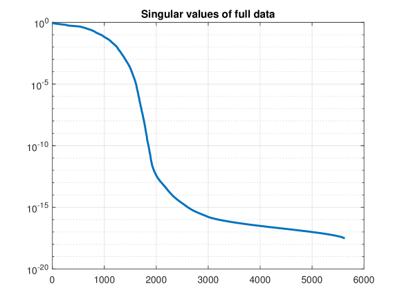
Figure 2.2: Singular values of the Lead field matrix on a logarithmic scale. The Lead field matrix uses $110\times 120=13200$ measurements for $75^{2}=5625$ unknowns. The rapid decay of the singular values is due to the severe ill-conditioning of the matrix. Increasing the number of measurements results in a similar rapid decay which indicates the inherent ill-posedness of the inverse problem.

2.2 Sequential coil activation

In ME-MRX, the volume is (partially) surrounded by an array of excitation coils and sensor arrays (see Figure 2.1). The coils can be steered to generate different types of activation fields. In the following we denote by $\mathbf{H}_{1},\dots,\mathbf{H}_{N_{c}}$ the magnetic fields induced by individual activation of the coils. Further, we write $\mathbf{b}_{c}\triangleq\mathbf{b}^{\mathbf{H}_{c}}\in\mathbb{R}^{N_{s}}$ and $\mathcal{L}_{c}\triangleq\mathcal{L}^{\mathbf{H}_{c}}\in\mathbb{R}^{N_{s}\times N_{v}}$ for the data and the Lead field matrix according to (2.2) and (2.3), corresponding to the activation field $\mathbf{H}=\mathbf{H}_{c}$. The measurements from all activations can be combined to a single equation of the form

$$\mathbf{b}=\mathcal{L}\,\mathbf{n}\in\mathbb{R}^{N_{c}N_{s}}\,,$$ (2.4)

where

$$\mathbf{b}\triangleq\begin{bmatrix}\mathbf{b}_{1}\\ \rule{10.00002pt}{0.5pt}\\ \vdots\\ \rule{15.00002pt}{0.5pt}\\ \mathbf{b}_{N_{c}}\end{bmatrix}\in\mathbb{R}^{N_{c}N_{s}}\quad\text{ and }\quad\;\mathcal{L}\triangleq\begin{bmatrix}\mathcal{L}_{1}\\ \rule{10.00002pt}{0.5pt}\\ \vdots\\ \rule{10.00002pt}{0.5pt}\\ \mathcal{L}_{N_{c}}\end{bmatrix}\in\mathbb{R}^{N_{c}N_{s}\times N_{v}}\,.$$ (2.5)

We will refer to $\mathbf{b}$ in (2.4) as full activation data. Evaluating (2.4) constitutes the forward model of ME-MRX. The corresponding inverse problem consists in determining the MNP distribution $\mathbf{n}\in\mathbb{R}^{N_{v}}$ from the data vector $\mathbf{b}$ that is additionally corrupted by noise. Note that Eq. (2.4) is known to be severely ill-conditioned as its singular values are rapidly decreasing (see [2]; an analysis in the infinite-dimensional setting has been performed in [13]). In Figure 2.2 we plot the singular values of the forward matrix for full data. The singular values decay rapidly. This reflects the severe ill-conditioning and implies that only a small number of singular components can be robustly reconstructed.

The multiple coil setup has been realized in [1, 30] and shown to significantly improve the spatial resolution compared to a single coil activation [30]. However, consecutive activations lead to a more time consuming measurement process. In order to accelerate data acquisition and to improve imaging resolution, we use CS techniques and develop a Douglas-Rachford based sparse reconstruction algorithm.

2.3 Compressive coil activations

The basic idea to employ CS for ME-MRX is to use $m$ specific coil activations, with $m\ll N_{c}$, instead of activating all $N_{c}$ coils in a sequential manner. Because of linearity, the data corresponding to the $j$th random activation pattern are given by

$$\mathbf{y}_{j}=\sum_{c=1}^{N_{c}}a_{j,c}\mathbf{b}_{c}=\sum_{c=1}^{N_{c}}a_{j,c}(\mathcal{L}\mathbf{n})_{c}+\boldsymbol{\xi}_{j}\quad\text{ for }j=1,\dots,m\,.$$ (2.6)

Here $\boldsymbol{\xi}_{j}$ models the error in the data and $a_{j,c}$ is the contribution of coil $N_{c}$ to the $j$th activation pattern. The measurement matrix

$$\mathbf{A}\triangleq\begin{pmatrix}a_{1,1}&\cdots&a_{1,N_{c}}\\ \vdots&&\vdots\\ a_{m,1}&\dots&a_{m,N_{c}}\end{pmatrix}\in\mathbb{R}^{m\times N_{c}}$$ (2.7)

represents all activation patters. Typical choices for $\mathbf{A}$ are Bernoulli or Gaussian matrices, since they are known to guarantee stable recovery of sparse signals [14]. Such kind of measurements can be naturally realized for ME-MRX, by simultaneous activation of several coils. The corresponding image reconstruction problem consists in recovering the MNP distribution $\mathbf{n}$ from the data in (2.6).

2.4 Matrix formulation of the reconstruction problem

In order to write the reconstruction problem in a compact form we introduce some additional notation. First, we define the CS measurement vector as

$$\mathbf{y}\triangleq\begin{bmatrix}\mathbf{y}_{1}\\ \rule{15.00002pt}{0.5pt}\\ \vdots\\ \rule{15.00002pt}{0.5pt}\\ \mathbf{y}_{m}\end{bmatrix}\in\mathbb{R}^{mN_{s}}\,.$$ (2.8)

Second, we introduce the vectorization or reshaping operator $\operatorname{vec}_{N_{c}}$, that takes a matrix to a vector whose block entries are equal to the transposes of the rows of the matrix:

$$\operatorname{vec}_{N_{c}}\colon\mathbb{R}^{N_{c}\times N_{s}}\to\mathbb{R}^{N_{c}N_{s}}\colon\mathbf{X}\mapsto\begin{bmatrix}\mathbf{X}_{1,-}^{\mathsf{T}}\\ \rule{15.00002pt}{0.5pt}\\ \vdots\\ \rule{15.00002pt}{0.5pt}\\ \mathbf{X}_{N_{c},-}^{\mathsf{T}}\end{bmatrix}\,.$$ (2.9)

We denote by $\operatorname{mat}_{N_{c}}$ the inverse reshaping operation that maps a vector in $\mathbb{R}^{N_{c}N_{s}}$ to a matrix in $\mathbb{R}^{N_{c}\times N_{s}}$. Further, we write $\mathbf{Y}\triangleq\operatorname{mat}_{m}\mathbf{y}$ and $\mathbf{B}\triangleq\operatorname{mat}_{N_{c}}\mathbf{b}$.

With the above notations, the CS data in (2.6) can be written in the compact form

$$\mathbf{Y}=\mathbf{A}\,\mathbf{L}\,\mathbf{n}+\boldsymbol{\Xi}\in\mathbb{R}^{m\times N_{s}}\,,$$ (2.10)

where $\mathbf{L}$ is the reshaped Lead field matrix defined by the property $\mathbf{L}\mathbf{n}=\operatorname{mat}_{N_{c}}(\mathcal{L}\mathbf{n})$ and $\boldsymbol{\Xi}$ denotes the noise matrix. With the Kronecker (or tensor) product $\mathcal{A}\triangleq\mathbf{A}\otimes\mathcal{I}\in\mathbb{R}^{(mN_{s})\times(N_{c}N_{s})}$ between the CS activation matrix $\mathbf{A}$ and the identity matrix $\mathcal{I}\in\mathbb{R}^{N_{s}\times N_{s}}$, equation (2.10) can further be rewritten in the form

$$\mathbf{y}=\mathcal{A}\,\mathcal{L}\,\mathbf{n}+\boldsymbol{\xi}\in\mathbb{R}^{mN_{s}}\,.$$ (2.11)

The image reconstruction task in CS ME-MRX consists in recovering the MNP distribution $\mathbf{n}$ from equation (2.10) or, equivalently, from equation (2.11).

3 Douglas-Rachford algorithm for CS MRX imaging

In order to recover the MNP distribution, the inverse problem (2.10) (or (2.11)) has to be solved which is known to be severely ill-posed, see Figure 2.2. We note that no standard approach for image reconstruction combining compressive measurements and severely ill-posed problems exist. This section is also of interest from a general perspective on CS for inverse problems.

3.1 Sparse Tikhonov regularization

We consider (2.11) as a single inverse problem with system matrix $\mathcal{M}=\mathcal{A}\mathcal{L}$. To address instability and non-uniqueness and to incorporate prior knowledge, we use a sparse regularization approach. For that purpose, we minimize the generalized Tikhonov functional [28]

$$\mathcal{T}_{\alpha,\beta}^{\mathcal{M}}(\mathbf{n})\triangleq\frac{1}{2}\|\mathbf{y}-\mathcal{M}\mathbf{n}\|_{2}^{2}+\alpha\|\boldsymbol{\Psi}\mathbf{n}\|_{1}+\beta\mathcal{R}(\mathbf{n})\,.$$ (3.1)

Here $\boldsymbol{\Psi}\colon\mathbb{R}^{N_{v}}\to\mathbb{R}^{d}$ is a transform that sparsifies the MNP concentration (with the $d\in\mathbb{N}$ the dimension of the transformed domain), $\mathcal{R}\colon\mathbb{R}^{N_{v}}\to[0,\infty)$ is an additional regularizer that incorporates additional prior knowledge about the MNP distribution (such as positivity and other convex constraints) and $\|\,\cdot\,\|_{p}$ is the standard $\ell^{p}$-norm defined by

$$\|\mathbf{x}\|_{p}\triangleq\sqrt[p]{\sum_{i=1}^{d}|x_{i}|^{p}}\quad\text{ for }\mathbf{x}=(x_{1},\dots,x_{d})\in\mathbb{R}^{d}\,.$$

The non-negative parameters $\alpha$ and $\beta$ allow to balance between the data consistency term $\frac{1}{2}\|\mathbf{y}-\mathcal{M}\mathbf{n}\|_{2}^{2}$, the sparsity prior $\|\boldsymbol{\Psi}\mathbf{n}\|_{1}$ and the additional regularizer $\mathcal{R}(\mathbf{n})$.

We call $\boldsymbol{\Psi}$ a sparsifying transform if $\boldsymbol{\Psi}\mathbf{n}$ can well be approximated by $k$-sparse vectors $\mathbf{x}$, defined by the property that $\{i\mid x_{i}\neq 0\}$ has at most $k$ elements. This approximation be can be quantified using the $k$-term approximation error,

$$\sigma_{k}(\mathbf{n})\triangleq\inf\{\|\mathbf{n}-\mathbf{n}_{k}\|_{1}\mid\mathbf{n}_{k}\textnormal{ is $k$-sparse}\}.$$ (3.2)

The $k$-term approximation error $\sigma_{k}(\mathbf{n})$ appears as additive term in standard error estimates in compressed sensing theory. For a mathematically precise discussion of the $k$-term approximation error we refer to [14].

Remark 1 (Recovery theory for (3.1)).

The $k$-restricted isometry property ($k$-RIP) of $\mathcal{M}=\mathcal{A}\mathcal{L}$ (after appropriate scaling) is defined as the smallest number $\delta_{k}$ such that for all $k$-sparse vectors $\boldsymbol{\Psi}\mathbf{n}$ we have

$$(1-\delta_{k})\|\mathbf{n}\|_{2}^{2}\leq\|\mathcal{M}\mathbf{n}\|_{2}^{2}\leq(1+\delta_{k})\|\mathbf{n}\|_{2}^{2}\,.$$ (3.3)

Roughly spoken, CS theory [5, 14] predicts uniform stable recovery with (3.1) for $\beta=0$ and in the sense that it stably recovers any $s$-sparse vector provided that the $s$-RIP constant of $\mathcal{M}$ is sufficiently small.

Due to the severe ill-conditioning of the Lead field matrix $\mathcal{L}$, the $s$-RIP is expected to be at most satisfied when the number $N_{v}$ of voxels is small. Figure 2.2 shows that the singular values of $\mathcal{L}$ with $N_{v}=5625$ are rapidly decaying and therefore the estimate $(1-\delta_{k})\|\mathbf{n}\|_{2}^{2}\leq\|\mathcal{M}\mathbf{n}\|_{2}^{2}$ for reasonable $\delta_{k}$ can only be satisfied for signals mainly formed by the first singular vectors. This implies that even in the case of full measurement data, where $\mathcal{A}$ is the identity matrix, uniform stable reconstruction of all sparse vectors is impossible. To obtain quantitative error estimates for (3.1), stable recovery results for individual elements [15, 16, 17] are a promising alternative. Such theoretical investigations are beyond the scope of this paper and an interesting line of future research.

Standard CS theory requires orthogonality of the sparsifying transform, which means that $\boldsymbol{\Psi}^{\mathsf{T}}\boldsymbol{\Psi}$ equals the identity matrix. Total variation (TV)-regularization [29] uses the gradient as sparsifying transform which is non-orthogonal. As in other compressed sensing imaging applications [21, 26] we observed TV to outperform orthogonal sparsifying transforms. We will therefore focus on TV and, due to space limitations, no results for orthogonal bases like wavelets are included.

3.2 Douglas-Rachford algorithm

In order to minimize (3.1), we propose using the Douglas-Rachford minimization algorithm, which is a backward-backward type splitting method for minimizing the sum $F+G$ of two functionals $F$ and $G$. For our purpose we take

$$F(\mathbf{n}) \triangleq\frac{1}{2}\|\mathbf{y}-\mathcal{M}\mathbf{n}\|_{2}^{2}$$ (3.4)

$$G(\mathbf{n}) \triangleq\alpha\|\boldsymbol{\Psi}\mathbf{n}\|_{1}+\beta\mathcal{R}(\mathbf{n})\,.$$ (3.5)

Minimizing (3.1) by the Douglas-Rachford algorithm, generates a sequence $(\mathbf{n}_{k})_{k\in\mathbb{N}}$ of estimated MNP distributions and auxiliary sequences $(\mathbf{z}_{k})_{k\in\mathbb{N}}$, $(\tilde{\mathbf{z}}_{k})_{k\in\mathbb{N}}$ as described in Algorithm A. See Section 4.1, for a discussion of the role of the parameter $\mu$.

Algorithm A Proposed sparse reconstruction algorithm for CS ME-MRX.

1:  Select $s\in(0,2)$, and $\mu>0$

2:  Initialize $\mathbf{z}_{0}=0$

3:  for  $k=1,\dots,N_{\rm iter}$ do

4:     $\mathbf{n}_{k}\leftarrow(\mathcal{M}^{\mathsf{T}}\mathcal{M}+\mu\mathcal{I})^{-1}(\mathcal{M}^{\mathsf{T}}\mathbf{y}+\mu\mathbf{z}_{k})$

5:     $\tilde{\mathbf{z}}_{k}\leftarrow\mathrm{argmin}_{\tilde{\mathbf{z}}}\frac{\mu}{2}\|(2\mathbf{n}_{k}-\mathbf{z}_{k})-\tilde{\mathbf{z}}\|_{2}^{2}+G(\tilde{\mathbf{z}})$

6:     $\mathbf{z}_{k+1}\leftarrow\mathbf{z}_{k}+s(\tilde{\mathbf{z}}_{k}-\mathbf{n}_{k})$

7:  end for

The Douglas-Rachford algorithm is a splitting type algorithm for minimizing $F+G$ which alternately performs updates according for $F$ (in our case, the residual functional or data fitting term) and $G$ (in our case, the regularizer). Because the regularizing term is non-smooth, standard methods such as Newton type methods cannot be applied. Splitting type methods are a natural choice in this case, and the implicit step in line 5 in Algorithm A accounts for the non-smoothness of $G$. Other splitting algorithms that are well suited to treat the non-smooth regularizer are the forward-backward splitting algorithm [10] and the Chambolle-Pock algorithm [6]. These algorithms use explicit gradient updates for the data fitting term requiring a matrix inversion. Therefore, they are not applicable to ME-MRX imaging. The Douglas-Rachford algorithm performs an implicit update for the data fitting term (line 4 Algorithm A), which is recognized as quadratic Tikhonov regularization step for the given equation and potentially accelerates the iteration.

For our numerical experiments, we take $\boldsymbol{\Psi}=\nabla$ as the discrete gradient operator as appropriate sparsifying transform for piecewise smooth MNP distributions. The additional regularizer is taken as the indicator function $\mathcal{R}=I_{C}$ of the convex set

$$C\triangleq\{\mathbf{n}\mid\forall\mathbf{r}_{v}\colon 0\leq n(\mathbf{r}_{v})\leq n_{\rm max}\}\quad\text{ for some bound }n_{\rm max}\,,$$

defined by $I_{C}(\mathbf{n})=0$ if $\mathbf{n}\in C$ and $I_{C}(\mathbf{n})=\infty$. It guarantees non-negativity and boundedness. With the above choices, the Tikhonov functional (3.1) reduces to total variation (TV) regularization with positivity constraint. The minimization of $\frac{\mu}{2}\|\mathbf{n}-\mathbf{z}\|_{2}^{2}+\|\nabla\mathbf{z}\|_{1}+i_{C}(\mathbf{z})$ required for implementing Algorithm A is a TV denoising step and again performed by the Douglas-Rachford algorithm using the decomposition in $F(\mathbf{z})=\frac{\mu}{2}\|\mathbf{n}-\mathbf{z}\|_{2}^{2}+\|\nabla\mathbf{z}\|_{1}$ and $G(\mathbf{z})=i_{C}(\mathbf{z})$.

Under the reasonable assumptions that the regularizer $G$ is lower semicontinuous and convex, and that the sparse Tikhonov functional $\mathcal{T}_{\alpha,\beta}^{\mathcal{M}}$ is coercive, the sequence $(\mathbf{n}_{k})_{k\in\mathbb{N}}$ generated by Algorithm A is known to converge to a minimizer of (3.1); see [10, 31]. Recall that the functional $G$ is called lower semicontinuous if $G(\mathbf{n})\leq\lim_{k\to\infty}G(\mathbf{n}_{k})$ for any $\mathbf{n}$ and any sequence $(\mathbf{n}_{k})_{k\in\mathbb{N}}$ converging to $\mathbf{n}$. Note that Algorithm A performs implicit steps with respect to the residual functional $F=\frac{1}{2}\|\mathcal{M}\mathbf{n}-\mathbf{y}\|_{2}^{2}$, which we found to have much faster convergence than forward-backward splitting algorithm [10]

$$\mathbf{z}_{k} \triangleq\mathbf{n}_{k}-\mathcal{M}^{\mathsf{T}}(\mathcal{M}\mathbf{n}_{k}-\mathbf{y})$$ (3.6)

$$mnp_{k} \triangleq\mathrm{argmin}_{\mathbf{n}}\frac{\mu}{2}\|\mathbf{z}_{k}-\mathbf{n}\|_{2}^{2}+G(\mathbf{n})\,$$ (3.8)

where $\mathbf{z}_{k}$ are auxiliary quantities and $\mathbf{n}_{k}$ the reconstructed MNPs.

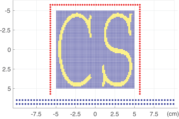
Figure 3.1: Full data setup for the numerical simulations. The phantom is contained in a square region of interest, the sensors are arranged in two parallel layers (blue dots), and the coils for full activation are arranged around the phantom in U-form (red dots).

4 Numerical results

For the following numerical simulations, we use a data setup similar to the realization in [1]. For simplification, we consider a two-dimensional setup representing one voxel plane, containing two parallel arrays of detector elements (one measuring the horizontal $(1,0)$ and one measuring the vertical $(0,1)$ component) located outside a quadratic region of interest. Circular shaped activation coils are arranged in U-form around the region of interest, all having the same normal vector $(0,1)$. The used arrangement of sensor and coil locations for the full measurement data setup is shown in Figure 3.1. For our simulations, we choose a discretization of imaging space into $N_{v}=75^{2}$ voxels covering a region of interest of $[-5,5]\times[-5,5]$ $\mathrm{c}\mathrm{m}^{2}$. The data are generated for $N_{s}=110$ positions and full measurement data correspond to $N_{c}=120$ activation coils outside the region of interest.

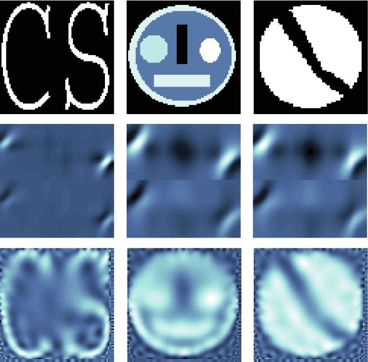
Figure 4.1: Phantoms, data and full measurement data reconstruction. Top row: CS-phantom (left), smiley-phantom (middle) and tumor-phantom mimicking cancerous tissue with included blood vessel (right). Middle row: Corresponding full measurement data. Bottom row: Reconstructions from full measurement data using standard quadratic Tikhonov regularization.

4.1 Forward computations

To set up the forward model (2.2), (2.4), (2.5), we first have to compute the magnetic fields generated by each coil. For that purpose, we follow the approach of [3, 1], where any circular activation coil is approximated by short line segments, each carrying the same current $I_{0}$. Every coil is modeled by 45 line segments for numerical calculations of the magnetic field. This is considered to be a sufficiently accurate approximation since the deviation of only 36 line segments from the analytical solution was shown to be already below $1\text{\,}\mathrm{\char 37\relax}$ in [22]. Using this approximation, the induced magnetic field at the voxel center $\mathbf{r}_{v}$ can be computed by (see [20])

$$\mathbf{H}(\mathbf{r}_{v})\simeq\frac{1}{4\pi}\sum_{i=1}^{45}\frac{|\mathbf{r}_{1,v,i}|+|\mathbf{r}_{2,v,i}|}{|\mathbf{r}_{1,v,i}|\,|\mathbf{r}_{2,v,i}|}\cdot\frac{\mathbf{r}_{1,v,i}\times\mathbf{r}_{2,v,i}}{|\mathbf{r}_{1,v,i}|\,|\mathbf{r}_{2,v,i}|+\mathbf{r}_{1,v,i}\mathchoice{\mathbin{\vbox{\hbox{\scalebox{0.6}{$\displaystyle\bullet$}}}}}{\mathbin{\vbox{\hbox{\scalebox{0.6}{$\textstyle\bullet$}}}}}{\mathbin{\vbox{\hbox{\scalebox{0.6}{$\scriptstyle\bullet$}}}}}{\mathbin{\vbox{\hbox{\scalebox{0.6}{$\scriptscriptstyle\bullet$}}}}}\mathbf{r}_{2,v,i}}\;I_{0}\,,$$ (4.1)

where $\mathbf{r}_{1,v,i}$ and $\mathbf{r}_{2,v,i}$ are the distance vectors between the voxel center $\mathbf{r}_{v}$ and the beginning and end points of the $i$th line segment, respectively. For the presented numerical computations, we use a coil diameter of $1\text{\,}\mu\mathrm{m}$, illustrating an almost point like coil. Having computed the activation field $\mathbf{H}(\mathbf{r}_{v})$, we compute the entries of the Lead field matrix according to (2.3). By activating the coils sequentially, we obtain the full measurement data Lead field matrix.

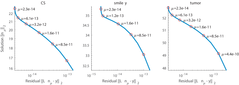
Figure 4.2: Selection of the regularization parameter by the L-curve method. Each image shows a log-log plot of the residual functionals versus the solution norm in dependence of the regularization parameter. The L-curve method predicts an L-shaped curve and advices to select a regularization parameter close to the corner of the L-curve. In our results we empirically found that taking the regularization parameter slightly smaller than advised by the L-curve method yield more accurate results.

For the presented results, we use three different magnetic particle distributions which, together with the corresponding measurements full data, are shown in Figure 4.1. Any column in the measurement data (in Figure 4.1 and below) corresponds to a single activation pattern and contains the data of all detectors. The phantoms are rescaled to have maximum value 1 and the forward operator $\mathcal{L}$ is rescaled to have matrix norm $\|\mathcal{L}\|_{2}=1$. To all data we have added additive Gaussian noise amounting to a signal-to-noise (SNR) of $80\text{\,}\mathrm{d}\mathrm{B}$. The corresponding reconstructions

$$\mathbf{n}_{\mu}=(\mathcal{L}^{\mathsf{T}}\mathcal{L}+\mu\mathcal{I})^{-1}\mathcal{L}^{\mathsf{T}}\mathbf{b}$$ (4.2)

with standard quadratic Tikhonov regularization (penalized least squares) using regularization parameter $\mu=10^{-12}$ are shown in the bottom row of Figure 4.1. Recall that $\mathcal{L}\in\mathbb{R}^{N_{c}N_{s}\times N_{v}}$ is the full Lead field matrix and $\mathbf{b}\in\mathbb{R}^{N_{c}N_{s}}$ the full activation data. Reconstructions with (4.2) can be seen as benchmark for the more sophisticated CS reconstructions applied to less data presented below. The regularization parameter has been chosen empirically as the trade-off between stability and smoothing. Taking a smaller regularization parameter would not suppress the noise (amplification) well enough, whereas a larger regularization parameter yields to overshooting. There are many strategies for selecting the regularization parameter analytically [19]. An example is the L-curve method, where the residual $\|\mathcal{L}\mathbf{n}_{\mu}-\mathbf{y}\|_{2}^{2}$ is plotted against the solution norm $\|\mathbf{n}_{\mu}\|$ both on a logarithmic scale. The L-curve method predicts the graph to be an L-shaped curve and the regularization parameter should be taken close to the corner of the L-shaped curve. The L-curves for the considered phantoms are plotted in Figure 4.2. Indeed, the selected $\mu=10^{-12}$ are close to the corner in each case. Strictly taken, the L-curve method predicts a larger regularization which we however found to yield to a slight over-smoothing and a larger reconstruction error.

The CS forward matrix $\mathcal{M}=\mathcal{A}\mathcal{L}$ is computed by multiplying the full Lead field matrix with $\mathcal{A}$. CS measurements have been generated in two random ways and one deterministic way. In the random case, $\mathbf{A}$ is taken either as Bernoulli matrix having entries $\pm 1$ appearing with equal probability, or a Gaussian matrix consisting of i.i.d. $\mathcal{N}(0,1)$-Gaussian random variables in each entry. The deterministic sparse sampling is performed by choosing $m$ equispaced coil activations.

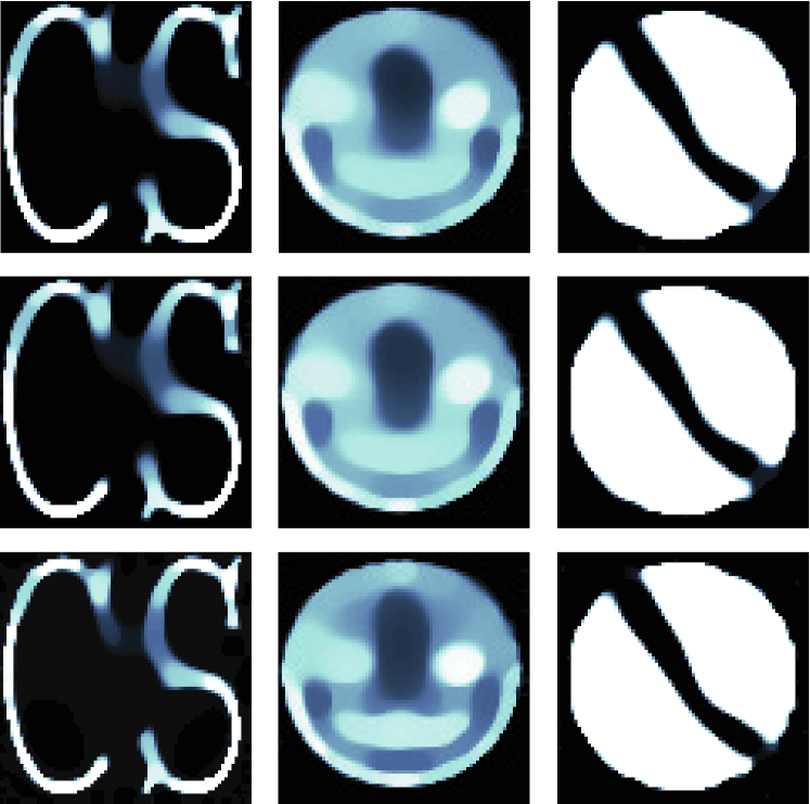
Figure 4.3: Reconstruction results with Algorithm A from 40 coil activations. Top row: Gaussian activation matrix. Middle row: Bernoulli activation matrix. Bottom row: Deterministic activation pattern.

	relative RMSE $(\%)$	SNR (dB)	correlation
40 Gaussian activations (proposed algorithm)
CS-phantom	0.75	2.51	0.92
smiley-phantom	0.40	8.05	0.87
tumor-phantom	0.16	15.69	0.98
40 Bernoulli activations (proposed algorithm)
CS-phantom	0.78	2.15	0.88
smiley-phantom	0.39	8.11	0.87
tumor-phantom	0.17	15.56	0.98
40 deterministic activations (proposed algorithm)
CS-phantom	0.66	3.59	0.92
smiley-phantom	0.35	9.16	0.90
tumor-phantom	0.17	15.38	0.98
120 activations (Tikhonov regularization)
CS-phantom	1.20	-1.59	0.69
smiley-phantom	0.47	6.45	0.80
tumor-phantom	0.35	8.99	0.89

Table 1: Evaluation metrics for Gaussian measurements (row 1) Bernoulli measurements (row 2) and deterministic activation pattern (row 3) using 40 activation patterns. The bottom row shows the same evaluation metrics for Tikhonov regularization for full activations.

4.2 Reconstruction results

The system matrix $\mathcal{M}$ is rescaled to have matrix norm 1 and we use the parameter setting $\mu=4\cdot 10^{-13}$, $\alpha=10^{-14}$, $s=1$, $n_{\rm max}=1$ and $N_{\rm iter}=50$. Note that the parameter $\mu$ has a similar role for each iterative step as in quadratic Tikhonov regularization (4.2). Choosing it too small causes noise amplification. Choosing it too large causes oversmoothing, which however will be reduced during the iteration. Therefore, taking it somewhat larger than the value found in Tikhonov case seems reasonable. The regularization parameter $\alpha$ has been selected empirically to yield good numerical performance.

We observed that after 50 iterations the reconstructed MNP stagnates which indicates that the iterates are close to the minimizer of the Tikhonov functional. The reconstructed MNP distributions using Algorithm A from 40 coil activations are shown in Figure 4.3. Each reconstruction takes about 50 seconds in Matlab R 2017a on a MacBook Pro (2016) with 2.9 GHz Intel Core i7 processor.

To quantitatively evaluate the reconstruction results, we compute the relative root mean squared error (RMSE) $\|\mathbf{n}-\mathbf{n}_{\rm rec}\|/\|\mathbf{n}\|$, the SNR $20\lg(\|\mathbf{n}\|/\|\mathbf{n}-\mathbf{n}_{\rm rec}\|)$, and the Pearson correlation coefficient $\operatorname{cov}(\mathbf{n},\mathbf{n}_{\rm rec})/\sqrt{\operatorname{var}(\mathbf{n})\operatorname{var}(\mathbf{n}_{\rm rec})}$ with $\operatorname{cov}$ denoting the covariance and $\operatorname{var}$ the variance. The results are shown in Table 1. For all phantoms and for any evaluation metric, the proposed algorithm clearly outperforms quadratic Tikhonov regularization. More specifically, the RSME for the proposed algorithm applied with 40 activations yields half of the RSME compared to quadratic Tikhonov regularization with 120 activations. For the CS-phantom and the smiley-phantom, the deterministic scheme performs best and decreases the reconstruction error by more than $10\text{\,}\mathrm{\char 37\relax}$ compared to the random schemes. For the tumor phantom, all sampling schemes yield comparable performance.

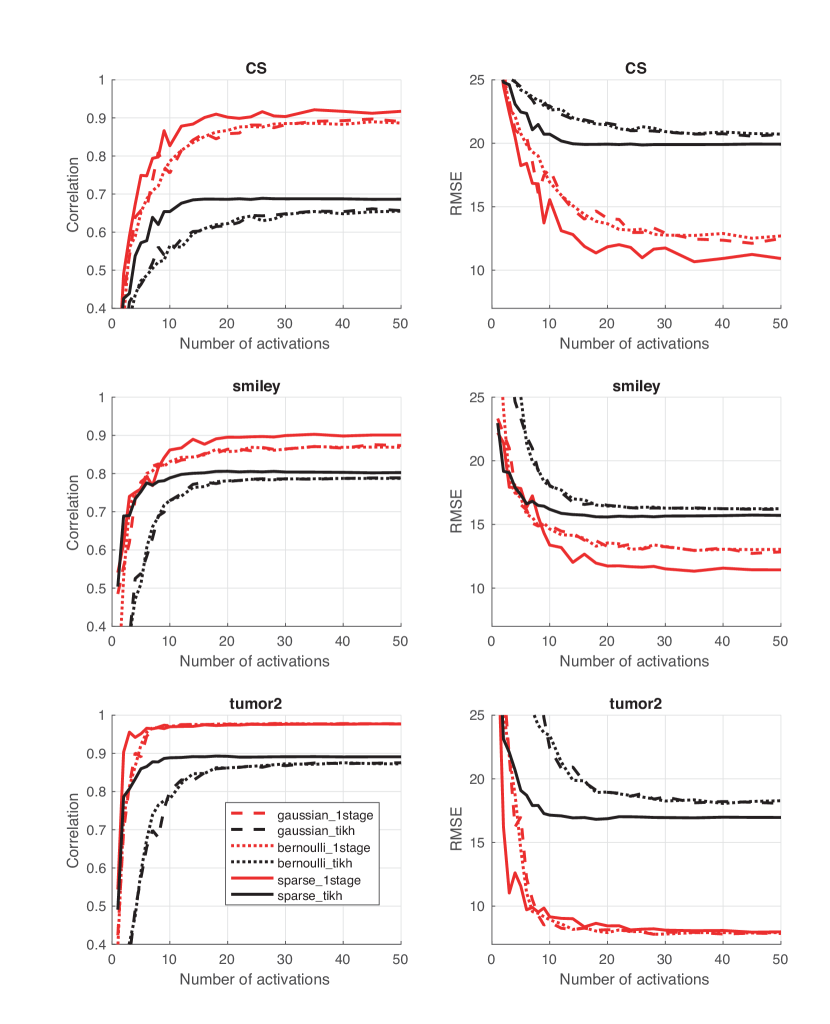
Figure 4.4: Quality evaluation in dependence of the number of coil activations. Left: correlation between reconstructions and the true phantoms. Right: RMSE of the reconstructions.

Figure 4.4 shows a convergence study (for the correlation and the RMSE) in dependence of the number of activations. We see that the Douglas-Rachford algorithm constantly outperforms Tikhonov regularization and significantly reduces the RSME and increases the correlation. For the CS and the smiley phantom, the deterministic sampling pattern has a significantly smaller RMSE than the random schemes. We address this behavior to the strong smoothing effect of the forward operator, which removes most high frequency components in the data. In the full forward matrix $\mathbf{A}\,\mathbf{L}$, the incoherence contained in the measurements matrix $\mathbf{A}$ is annihilated by the smoothing effect of $\mathbf{A}$. Finding particular activation patterns that outperform the sparse sampling scheme is a nontrivial issue and will be investigated in future work.

5 Conclusion

The use of multiple coil activation patterns in magnetorelaxometry imaging is time consuming and requires performing several consecutive measurements. It is therefore desirable to make the number of coil activations as small as possible, while keeping high spatial resolution. For that purpose, we investigated CS strategies in this paper. We compared Gaussian random activations, Bernoulli activations and deterministic sparse sampling schemes. For actual image reconstruction, we applied Douglas-Rachford splitting to the sparse Tikhonov functional; see Algorithm A. For a small number of coil activations, the random schemes slightly outperform the deterministic scheme for the smiley-phantom and tumor phantom. For a large number of activations, the deterministic sampling scheme clearly performed better than the random sampling patterns. We explain this behavior by the severe ill-conditioning of the Lead field matrix, which is more severe for a large number of activations. Only for a small number of activations, where the resolution is poor anyway, the incoherence at the low frequencies is not destroyed by the smoothing effect of the Lead field matrix. The reconstruction results clearly demonstrate the proposed Algorithm A significantly outperforms standard algorithms such as Tikhonov regularization. Depending on the complexity of the phantom between 6 (tumor) and 30 activations (CS) are sufficient for the used framework and further increasing the number of activations only decreases the RMSE by a few percent; see Figure 4.4.

Several interesting research directions following this work are possible. First, we can replace the inner TV minimization in the single-stage approach by a different algorithm which should accelerate Algorithm A. Second, the derivation of theoretical error estimates for the single-stage approach is of significant interest. Results in that direction can advise which type of MRX measurements are best to obtain accurate results for certain phantom classes. Moreover, the derivation of adaptive compressed sensing strategies for online monitoring is of significant interest. Advising optimal coil activations given previous activations is a practically important challenge that will benefit from theoretical error estimates, numerical simulations as well as real-world experiments. Such issues will be addressed in future work. In this paper, we investigated standard random compressed sensing schemes (using Gaussian and Bernoulli activation patterns and sparse sampling). Using more problem adapted and task oriented measurement design we expect to derive improved coil activation schemes.

References

- [1] D. Baumgarten, F. Braune, E. Supriyanto, and J. Haueisen. Plane-wise sensitivity based inhomogeneous excitation fields for magnetorelaxometry imaging of magnetic nanoparticles. J. Magn. Magn. Mater., 380:255–260, 2015.
- [2] D. Baumgarten, R. Eichardt, G. Crevecoeur, E. Supriyanto, and J. Haueisen. Magnetic nanoparticle imaging by random and maximum length sequences of inhomogeneous activation fields. In 35th Annual International Conference of the IEEE Engineering in Medicine and Biology Society (EMBC), pages 3258–3260, 2013.
- [3] D. Baumgarten and J. Haueisen. A spatio-temporal approach for the solution of the inverse problem in the reconstruction of magnetic nanoparticle distributions. IEEE Trans. Magn., 46(8):3496–3499, 2010.
- [4] D. Baumgarten, M. Liehr, F. Wiekhorst, U. Steinhoff, P. Münster, P. Miethe, L. Trahms, and J. Haueisen. Magnetic nanoparticle imaging by means of minimum norm estimates from remanence measurements. Med. Biol. Eng. Comput., 46(12):1177–1185, 2008.
- [5] E. J. Candès, J. K. Romberg, and T. Tao. Stable signal recovery from incomplete and inaccurate measurements. Comm. Pure Appl. Math., 59(8):1207–1223, 2006.
- [6] A. Chambolle and T. Pock. A first-order primal-dual algorithm for convex problems with applications to imaging. J. Math. Imaging Vision, 40(1):120–145, 2011.
- [7] G.-H. Chen, J. Tang, and S. Leng. Prior image constrained compressed sensing (PICCS): a method to accurately reconstruct dynamic CT images from highly undersampled projection data sets. Med. Phys., 35(2):660–663, 2008.
- [8] A. Coene, G. Crevecoeur, and L. Dupre. Adaptive control of excitation coil arrays for targeted magnetic nanoparticle reconstruction using magnetorelaxometry. IEEE Trans. Magn., 48(11):2842–2845, 2012.
- [9] A. Coene, J. Leliaert, M. Liebl, N. Loewa, U. Steinhoff, G. Crevecoeur, L. Dupré, and F. Wiekhorst. Multi-color magnetic nanoparticle imaging using magnetorelaxometry. Phys. Med. Biol., 62(8):3139, 2017.
- [10] P. L. Combettes and J.-C. Pesquet. Proximal splitting methods in signal processing. In Fixed-point algorithms for inverse problems in science and engineering, pages 185–212. Springer, 2011.
- [11] G. Crevecoeur, D. Baumgarten, U. Steinhoff, J. Haueisen, L. Trahms, and L. Dupré. Advancements in magnetic nanoparticle reconstruction using sequential activation of excitation coil arrays using magnetorelaxometry. IEEE Trans. Magn., 48(4):1313–1316, 2012.
- [12] D. L. Donoho. Compressed sensing. IEEE Trans. Inf. Theory, 52(4):1289–1306, 2006.
- [13] J. Föcke, D. Baumgarten, and M. Burger. The inverse problem of magnetorelaxometry imaging, 2018. arXiv:1802.05937.
- [14] S. Foucart and H. Rauhut. A mathematical introduction to compressive sensing. Birkhäuser Basel, 2013.
- [15] J. J. Fuchs. Recovery of exact sparse representations in the presence of bounded noise. IEEE Trans. Inf. Theory, 51(10):3601–3608, 2005.
- [16] M. Grasmair, M. Haltmeier, and O. Scherzer. Necessary and sufficient conditions for linear convergence of -regularization. Comm. Pure Appl. Math., 64(2):161–182, 2011.
- [17] M. Haltmeier. Stable signal reconstruction via -minimization in redundant, non-tight frames. IEEE Trans. Signal Process., 61(2):420–426, 2013.
- [18] M. Haltmeier, T. Berer, S. Moon, and P. Burgholzer. Compressed sensing and sparsity in photoacoustic tomography. J. Opt., 18(11):114004 (12 pages), 2016.
- [19] P. C. Hansen. Rank-Deficient and Discrete Ill-Posed Problems. SIAM Monographs on Mathematical Modeling and Computation. SIAM, Philadelphia, PA, 1998.
- [20] J. D. Hanson and S. P. Hirshman. Compact expressions for the Biot–Savart fields of a filamentary segment. Phys. Plasmas, 9(10):4410–4412, 2002.
- [21] F. Krahmer and R. Ward. Stable and robust sampling strategies for compressive imaging. IEEE Trans. Image Process., 23(2):612–622, 2014.
- [22] M. Liebl. Bildgebung von magnetischen nanopartikelverteilungen mit einem zylindrischen magnetisch geschirmten squid-system, 2011. Master’s thesis, Ilmenau University of Technology, Germany.
- [23] M. Liebl, U. Steinhoff, F. Wiekhorst, J. Haueisen, and L. Trahms. Quantitative imaging of magnetic nanoparticles by magnetorelaxometry with multiple excitation coils. Phys. Med. Biol., 59(21):6607, 2014.
- [24] M. Liebl, F. Wiekhorst, D. Eberbeck, P. Radon, D. Gutkelch, D. Baumgarten, U. Steinhoff, and L. Trahms. Magnetorelaxometry procedures for quantitative imaging and characterization of magnetic nanoparticles in biomedical applications. Biomed. Tech., 60(5):427–443, 2015.
- [25] M. Lustig, D. L. Donoho, J. M. Santos, and J. M. Pauly. Compressed sensing mri. IEEE Sig. Proc. Mag., 25(2):72–82, 2008.
- [26] C. Poon. On the role of total variation in compressed sensing. SIAM J. Imaging Sci., 8(1):682–720, 2015.
- [27] H. Richter, M. Kettering, F. Wiekhorst, U. Steinhoff, I. Hilger, and L. Trahms. Magnetorelaxometry for localization and quantification of magnetic nanoparticles for thermal ablation studies. Phys. Med. Biol., 55(3):623–633, 2010.
- [28] O. Scherzer, M. Grasmair, H. Grossauer, M. Haltmeier, and F. Lenzen. Variational methods in imaging, volume 167 of Applied Mathematical Sciences. Springer, New York, 2009.
- [29] O. Scherzer, M. Grasmair, H. Grossauer, M. Haltmeier, and F. Lenzen. Variational methods in imaging, volume 167 of Applied Mathematical Sciences. Springer, New York, 2009.
- [30] U. Steinhoff, F. Wiekhorst, D. Baumgarten, J. Haueisen, and L. Trahms. Imaging of magnetic nanoparticles based on magnetorelaxometry with sequential activation of inhomogeneous magnetization fields. Biomed. Tech., 55:22–25, 2010.
- [31] B. F. Svaiter. On weak convergence of the Douglas–Rachford method. SIAM J. Control Optim., 49(1):280–287, 2011.
- [32] F. Wiekhorst, C. Seliger, R. Jurgons, U. Steinhoff, D. Eberbeck, L. Trahms, and C. Alexiou. Quantification of magnetic nanoparticles by magnetorelaxometry and comparison to histology after magnetic drug targeting. J. Nanosci. Nanotechnol., 6(9-10):3222–3225, 2006.
- [33] F. Wiekhorst, U. Steinhoff, D. Eberbeck, and L. Trahms. Magnetorelaxometry assisting biomedical applications of magnetic nanoparticles. Pharm. Res., 29(5):1189–1202, 2012.