A Laminar Model for the Magnetic Field Structure in Bow-Shock Pulsar Wind Nebulae

Abstract

Bow Shock Pulsar Wind Nebulae are a class of non-thermal sources, that form when the wind of a pulsar moving at supersonic speed interacts with the ambient medium, either the ISM or in a few cases the cold ejecta of the parent supernova. These systems have attracted attention in recent years, because they allow us to investigate the properties of the pulsar wind in a different environment from that of canonical Pulsar Wind Nebulae in Supernova Remnants. However, due to the complexity of the interaction, a full-fledged multidimensional analysis is still laking. We present here a simplified approach, based on Lagrangian tracers, to model the magnetic field structure in these systems, and use it to compute the magnetic field geometry, for various configurations in terms of relative orientation of the magnetic axis, pulsar speed and observer direction. Based on our solutions we have computed a set of radio emission maps, including polarization, to investigate the variety of possible appearances, and how the observed emission pattern can be used to constrain the orientation of the system, and the possible presence of turbulence.

1 Introduction

Pulsars are rapidly rotating and strongly magnetized neutron stars (Gold, 1968; Pacini, 1967). Due to the interplay of a fast rotation and a strong magnetic field, a large induced electric field forms at their surface, capable of pulling electrons out of the crust (Goldreich & Julian, 1969), and driving a pair creation cascade process, that leads to the formation of a pair dominated outflow, known as pulsar wind (Ruderman & Sutherland, 1975; Arons & Scharlemann, 1979; Hibschman & Arons, 2001; Timokhin & Arons, 2013). This wind is accelerated beyond the Light Cylinder to high Lorentz factors. While the mechanism responsible of such acceleration is still poorly understood (Michel, 1973; Bogovalov, 1999; Kirk & Skjæraasen, 2003; Mochol, 2017), there is no doubt that at the typical distances where this wind is seen to interact with the environment, it is cold and likely endowed with a toroidal magnetic field, wound up around the pulsar spin-axis, and carrying a non-negligible fraction of the pulsar spin-down luminosity (Melatos, 1998).

The interaction of the pulsar wind with the surrounding environment gives rise to a Pulsar Wind Nebula (PWN) (Gaensler & Slane, 2006; Bucciantini, 2008; Olmi et al., 2016). A bubble of relativistic pairs and magnetic field, that shines with a non-thermal broad band spectrum, extending from radio to X-rays and $\gamma$-rays, via synchrotron and inverse Compton emission. The Crab nebula is the prototype of PWNe inside the parent Supernova Remnant (SNR) (Hester, 2008). Given that the typical pulsar speed at birth, the so called kick velocity, is usually of the order of $100-400$ km s^-1 (Cordes & Chernoff, 1998; Arzoumanian, Chernoff & Cordes, 2002; Sartore et al., 2010; Verbunt, Igoshev & Cator, 2017), much smaller than the expansion speed of young SNRs [typically a few thousands km s^-1 (Truelove & McKee, 1999; Hughes, 1999, 2000; DeLaney & Rudnick, 2003; Borkowski et al., 2013; Tsuji & Uchiyama, 2016)], for the first few thousands of years, the PWN is going to remain confined within the parent SNR (van der Swaluw et al., 2003; van der Swaluw, Downes & Keegan, 2004; Temim et al., 2015). However the SNR expansion speed will drop in time as the expansion proceeds (Cioffi, McKee & Bertschinger, 1988; Leahy, Green & Tian, 2014; Sánchez-Cruces et al., 2018), sweeping up more and more ISM material, such that on a typical timescale of a few tens of thousands of years, the pulsar can escape from the SNR, and begin to interact directly with the ISM. Given the typical sound speed of the ISM, the pulsar motion is highly supersonic, and the ram pressure balance between the pulsar wind and the ISM flow gives rise to a cometary-like nebula (Wilkin, 1996) known as Bow-Shock Pulsar Wind Nebula (BSPWN), of shocked pulsar and ISM material (Bucciantini & Bandiera, 2001; Bucciantini, 2002b). If the ISM is cold and its neutral fraction is high, these nebulae can be observed in H_α emission (Kulkarni & Hester, 1988; Cordes, Romani & Lundgren, 1993; Bell et al., 1995; van Kerkwijk & Kulkarni, 2001; Jones, Stappers & Gaensler, 2002; Brownsberger & Romani, 2014; Romani, Slane & Green, 2017), due to charge exchange and collisional excitation, taking place in the shocked ISM downstream of the forward bowshock (Chevalier, Kirshner & Raymond, 1980; Hester, Raymond & Blair, 1994; Bucciantini & Bandiera, 2001; Ghavamian et al., 2001), or alternatively in the UV (Rangelov et al., 2016), and IR (Wang et al., 2013). On the other hand the shocked pulsar material is expected to emit non-thermal synchrotron radiation, and indeed many such systems have been identified in recent years either in radio or in X-rays (Arzoumanian et al., 2004; Kargaltsev et al., 2017, 2008; Gaensler et al., 2004; Yusef-Zadeh & Gaensler, 2005; Li, Lu & Li, 2005; Gaensler, 2005; Chatterjee et al., 2005; Ng et al., 2009; Hales et al., 2009; Ng et al., 2010; De Luca et al., 2011; Marelli et al., 2013; Jakobsen et al., 2014; Misanovic, Pavlov & Garmire, 2008; Posselt et al., 2017; Klingler et al., 2016; Ng et al., 2012). There is also an interesting dichotomy between H_α emitting systems and synchrotron emitting ones, suggesting that energetic pulsars, more likely to drive bright synchrotron nebulae, might pre-ionize the incoming ISM suppressing line emission from neutral hydrogen.

Despite the fact that the study of BSPWNe dates back to almost two decades ago (Cordes, Romani & Lundgren, 1993; Bucciantini & Bandiera, 2001; Bucciantini, Amato & Del Zanna, 2005), in recent years there has been a renewed interest in these systems. In part due to an increasing number of discoveries in radio and X-rays, that have enlarged our sample and shown us the large variety of morphologies characterizing them, in part because pulsars are perhaps the most efficient antimatter factories in the Galaxy, and BSPWNe have been suggested as one of the major contributors to the positron excess observed by PAMELA (Adriani et al., 2009; Hooper, Blasi & Dario Serpico, 2009; Blasi & Amato, 2011; Adriani et al., 2013; Aguilar et al., 2013), in competition with dark matter (Wang, Pun & Cheng, 2006). In recent years the discovery of peculiar X-ray outflows in BSPWNe (Hui et al., 2012; Pavan et al., 2014) has also put into question or current understanding of pulsar winds (Spitkovsky, 2006; Tchekhovskoy, Spitkovsky & Li, 2013; Tchekhovskoy, Philippov & Spitkovsky, 2016), and the canonical MHD paradigm of PWNe (Rees & Gunn, 1974; Kennel & Coroniti, 1984a, b; Begelman & Li, 1992; Komissarov & Lyubarsky, 2004; Del Zanna, Amato & Bucciantini, 2004; Bogovalov et al., 2005; Volpi et al., 2008b; Porth, Komissarov & Keppens, 2014; Olmi et al., 2016; Del Zanna & Olmi, 2017). BSPWNe offer the unique opportunity to study the characteristic of pulsar injection in an environment where the typical flow timescales are short, compared to synchrotron cooling times, even in radio, such that one can safely assume that they trace the instantaneous injection conditions of the pulsar, as opposed to younger PWNe inside SNRs, where the contribution to the emission by particles injected during the entire lifetime of the system makes it harder to disentagle secular effects from instantaneous properties.

Unfortunately, once the structure of magnetized winds is included, the dynamics in BSPWNe will turn out to depend on a variety of different parameters: the anisotropy of the pulsar wind energy flux (Bandiera, 1993; Wilkin, 2000; Vigelius et al., 2007), the inclination of the spin axis with respect to the pulsar kick velocity (Johnston et al., 2005; Ng & Romani, 2007; Johnston et al., 2007; Noutsos et al., 2012, 2013), the magnetization of the pulsar wind (Bucciantini, Amato & Del Zanna, 2005), the presence and fate of a striped wind region (Mochol, 2017; Cerutti & Philippov, 2017; Porth, Komissarov & Keppens, 2014; Komissarov, 2013; Pétri & Lyubarsky, 2007; Del Zanna, Amato & Bucciantini, 2004), not to mention the conditions in the ISM, like its neutral fraction (Bucciantini, 2002c; Morlino, Lyutikov & Vorster, 2015). On top of this, if one wishes to model the observed properties, also the orientation of the observer’s direction needs to be taken into account, as well as the acceleration properties of the emitting particles (Olmi et al., 2014, 2015; Sironi & Spitkovsky, 2011, 2009). All of this makes a complete sampling of the possible parameter space, via brute force numerical simulations in the proper relativistic MHD regime, quite challenging. However, if one gives up capturing all the complexity of the dynamics of the flow, and retains only those key features that are supposed to characterize the average properties of the system, it is then possible to develop extremely simplified models, that can at least try to address the 3D structure of the magnetic field, and the expected non-thermal emission properties. These might serve both as a benchmark, with respect to full fledged numerical models, and as a starting point, to select those configurations that appear to be more interesting in the light of specific observables.

In this work we develop a formalism to transport the 3D magnetic field on a given stationary hydrodynamical configuration, and we apply it to the development of models of the magnetic field geometry for BSPWNe, which we then use to build emission maps, including polarization, in orded to understand the typical patterns one might observe in synchrotron emission.

This work is structured as follows: in Sect. 2 we introduce and describe the formalism we adopt to solve the induction equation for magnetic field evolution; in Sect. 3, we present the simplified flow structure that we have adopted for BSPWNe; in Sect 4 we detail how to relate the magnetic field structure in the nebula to the one in the pulsar wind, which is our injection site; in Sect 5 we present and discuss our results. Finally we conclude in Sect. 6.

2 Transport of a Solenoidal Vector Field

The equation that describes the evolution of the magnetic field $\boldsymbol{B}$, measured in the observer frame, in Ideal MHD is the induction equation:

$$\frac{\partial\boldsymbol{B}}{\partial t}=-\nabla\times\boldsymbol{E}=\nabla\times[\boldsymbol{v}\times\boldsymbol{B}]/c$$ (1)

where $\boldsymbol{E}$ is the electric field in the observer frame and $\boldsymbol{v}$ is the flow speed. Together with the solenoidal condition, $\nabla\cdot\boldsymbol{B}=0$, this equation can be written as:

$$\frac{D\boldsymbol{B}}{Dt}=\frac{\partial\boldsymbol{B}}{\partial t}+(\boldsymbol{v}\cdot\nabla)\boldsymbol{B}=(\boldsymbol{B}\cdot\nabla)\boldsymbol{v}-(\nabla\cdot\boldsymbol{v})\boldsymbol{B}$$ (2)

where $D/Dt$ represents the Lagrangian derivative of the field along the trajectory of a fluid element. This equation allows one to evolve the magnetic field along the flow, once the velocity field and its derivatives are known, and it is commonly adopted in Lagrangian schemes (Price & Monaghan, 2004; Rosswog & Price, 2007; Price, 2011). This equation however is not suitable when the velocity field develops strong discontinuities, like shocks, where the flow velocity is not properly defined, and local derivatives diverge. One can solve this problem either introducing some viscosity, and smoothing the shock jumps, or resorting to an integral version for the evolution of the magnetic field, which is the approach we adopt in this work.

The flux-freezing condition of Ideal MHD relates the evolution of the magnetic field to the way nearby fluid elements move with respect to one another, and in particular to the way their relative displacements evolve (see Fig. 1). Let us call $\boldsymbol{P}(t,\boldsymbol{P}_{o})$ the trajectory of a fluid element (the position of a fluid element that at $t=0$ was located in $\boldsymbol{P}_{o}$), and $\boldsymbol{B}(t,\boldsymbol{P}_{o})$ the magnetic field along the trajectory $\boldsymbol{P}(t,\boldsymbol{P}_{o})$ of that same fluid element at time $t$.

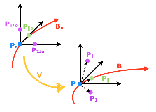
Figure 1: Schematic evolution of a fluid elements and its nearby fluid elements displaced either in the parallel or perpendicular directions. $\boldsymbol{P}=\boldsymbol{P}(t,\boldsymbol{P}_{o})$, $\boldsymbol{P}_{\parallel}=\boldsymbol{P}(t,\boldsymbol{P}_{\parallel o})$, $\boldsymbol{P}_{1\perp}=\boldsymbol{P}(t,\boldsymbol{P}_{1\perp o})$, $\boldsymbol{P}_{2\perp}=\boldsymbol{P}(t,\boldsymbol{P}_{2\perp o})$, and $\boldsymbol{B}_{o}=\boldsymbol{B}(0,\boldsymbol{P}_{o})$

Let us consider a point $\boldsymbol{P}_{\parallel\;0}=\boldsymbol{P}_{o}+\epsilon\boldsymbol{e}_{B}(0,\boldsymbol{P}_{o})$, where $\boldsymbol{e}_{B}(0,\boldsymbol{P}_{o})$ is a unitary vector parallel to the direction of the magnetic field at position $\boldsymbol{P}_{o}$ and time $t=0$. In the limit $\epsilon\rightarrow 0$, $\boldsymbol{P}_{\parallel\;0}$ represents a fluid element displaced by an amount $\epsilon$ from $\boldsymbol{P}_{o}$ along the local magnetic field. Ideal MHD ensures that the two fluid elements remain on the same magnetic field line. Then, to first order in $\epsilon$, the direction of the magnetic field in $\boldsymbol{P}(t,\boldsymbol{P}_{o})$ will be simply given by:

$$\boldsymbol{e}_{B}(t,\boldsymbol{P}_{o})=\frac{\boldsymbol{P}(t,\boldsymbol{P}_{\parallel\;o})-\boldsymbol{P}(t,\boldsymbol{P}_{o})}{|\boldsymbol{P}(t,\boldsymbol{P}_{\parallel\;o})-\boldsymbol{P}(t,\boldsymbol{P}_{o})|}$$ (3)

One can even define a second order accurate estimate of the magnetic field direction, by taking also a negative displacement by $-\epsilon$, and using a centered definition of the positional derivative:

$$\boldsymbol{e}_{B}(t,\boldsymbol{P})=\frac{\boldsymbol{P}(t,\boldsymbol{P}_{+\parallel\;o})-\boldsymbol{P}(t,\boldsymbol{P}_{-\parallel\;o})}{|\boldsymbol{P}(t,\boldsymbol{P}_{+\parallel\;o})-\boldsymbol{P}(t,\boldsymbol{P}_{-\parallel\;o})|}$$ (4)

where $\pm\parallel$ refers to an initial displacement of $\pm\epsilon$ respectively. Given an initial magnetic field loop, this equation allows one to trace the evolution of the loop in time, and to trace the related magnetic surface. The values of $\epsilon$ must be chosen in order to preserve in time the accuracy of the estimate. For example, it is well known that the displacement will diverge exponentially in a turbulent flow (Yamada & Ohkitani, 1987; Biferale et al., 2005; Yamada & Ohkitani, 1998; Salazar & Collins, 2009; Berera & Ho, 2018), while in a laminar flow it will likely remain bound.

On the other hand, in Ideal MHD, the evolution of the strength of the magnetic field $\boldsymbol{B}(t,\boldsymbol{P}_{o})$ along the fluid element trajectory $\boldsymbol{P}(t,\boldsymbol{P}_{o})$ is related to the evolution of the cross section of an infinitesimal magnetic flux tube centered on the same fluid element, $\Phi(t,\boldsymbol{P}_{o})$:

$$\frac{|\boldsymbol{B}(t,\boldsymbol{P}_{o})|}{|\boldsymbol{B}(0,\boldsymbol{P}_{o})|}=\frac{\Phi(0,\boldsymbol{P}_{o})}{\Phi(t,\boldsymbol{P}_{o})}$$ (5)

To trace the evolution of the cross section of an infinitesimal magnetic flux tube, one can follow the evolution of two fluid elements originally (at $t=0$) displaced in directions perpendicular to the magnetic field. Let $\boldsymbol{e}_{1\perp}$ and $\boldsymbol{e}_{2\perp}$ be unitary vectors such that:

$$\boldsymbol{e}_{1\perp}\cdot\boldsymbol{e}_{2\perp}=0,\quad\boldsymbol{e}_{1\perp}\cdot\boldsymbol{e}_{B}(0,\boldsymbol{P}_{o})=0,\quad\boldsymbol{e}_{2\perp}\cdot\boldsymbol{e}_{B}(0,\boldsymbol{P}_{o})=0,\!$$ (6)

then one can define two fluid elements originally displaced perpendicular to the local magnetic field as:

$$\boldsymbol{P}_{1\perp\;o}=\boldsymbol{P}_{o}+\epsilon\boldsymbol{e}_{1\perp}\quad\boldsymbol{P}_{2\perp\;o}=\boldsymbol{P}_{o}+\epsilon\boldsymbol{e}_{2\perp}$$ (7)

and the initial (at $t=0$) infinitesimal cross section of the flux tube at $\boldsymbol{P}_{o}$ as:

$$\Phi(0,\boldsymbol{P}_{o})=|(\boldsymbol{P}_{1\perp\;o}-\boldsymbol{P}_{o})\times(\boldsymbol{P}_{2\perp\;o}-\boldsymbol{P}_{o})|=\epsilon^{2}$$ (8)

In general, depending on the shear of the velocity field, the evolution of fluid elements originally displaced perpendicular to the magnetic field, will not keep them perpendicularly displaced. One however can redefine a perpendicular projection as:

$$\boldsymbol{\xi}_{1} =\boldsymbol{P}(t,\boldsymbol{P}_{1\perp\;o})-\boldsymbol{P}(t,\boldsymbol{P}_{o})+$$

$$\quad\quad-[(\boldsymbol{P}(t,\boldsymbol{P}_{1\perp\;o})-\boldsymbol{P}(t,\boldsymbol{P}_{o}))\cdot\boldsymbol{e}_{B}(t,\boldsymbol{P}_{o})]\boldsymbol{e}_{B}(t,\boldsymbol{P}_{o})$$ (9)

and similarly for $\boldsymbol{\xi}_{2}$. Then the infinitesimal flux tube cross section will be given by $\Phi(t,\boldsymbol{P}_{o})=|\boldsymbol{\xi}_{1}\times\boldsymbol{\xi}_{2}|$. Again it is possible to define a second order estimate for the evolution of the cross section of the flux tube, using displacements in both the positive and negative direction, and taking central differences in the definition of the $\boldsymbol{\xi}$ projections.

Given that the evolution of the trajectory of a fluid element, and of nearby displaced fluid elements, is simply given by the velocity field, and does not involve its derivatives, one can use this approach to trace the evolution of the magnetic field in the presence of discontinuities in the velocity as those expected in the case of shocks. Note moreover that this approach makes no assumption on the velocity field, excluding only those highly turbulent flows where nearby fluid elements rapidly drift apart. We have verified that on smooth differentiable flow fields this approach, based on displacments, gives equivalent results to direct integration of Eq. 2.

3 A Laminar Flow Model

In this section we describe the velocity field we used to model the transport of magnetic field in BSPWNe. We begin by briefly reviewing the key characteristics of BSPWNe. Let us place ourself in a reference frame centered on the PSR, with the $z-$axis aligned with the pulsar speed. In this reference frame the ISM is seen moving in the negative $z-$direction. Given the typical values of the pulsars’ velocity $\sim 100-400$ km s^-1, and the typical temperatures of the ISM $\sim 10^{4}-10^{5}$ K, such flow will be highly supersonic. The interaction of the relativistic pulsar wind with the incoming ISM, produces a cometary-like nebula of shocked pulsar wind and ISM material. Four regions can be identified in this system. With reference to Fig. 2, moving from the pulsar outward one finds:

• In inner region (A), containing the relativistic, magnetized and cold pulsar wind, which moves with high Lorentz factor in the radial direction.

• A cometary-like region (B) of pulsar wind material, which has been shocked, heated and slowed down to sub-relativistic speeds in a bullet shaped termination shock (TS). It is this region that is seen in non-thermal radio and X-rays synchrotron emission.

• A region (C) of ISM material shocked in a forward bow-shock, and separated from the former region B by a contact discontinuity (CD). This is the region usually observed in H_α emission.

• An outer region (D) occupied by the supersonic ISM flow.

Each one of these regions is separated from the other by sharp transitions, either a shock or a CD. Due to the balance between the ram pressure of the pulsar wind and the one of the incoming ISM, material in region B is forced to flow into a collimated tail. While in the head, the flow speed of region B is strongly subsonic, and just a small fraction of the speed of light, as it moves sideways toward the tail, it accelerates, becoming supersonic and reaching a speed as high as $0.7-0.8c$. Downstream of the Mach Disk that forms the back side of the wind termination shock, a low velocity inner channel develops. It is found in numerical simulations that this low velocity inner channel can extend up to twice the distance of the Mach Disk, where, due to the interaction with the faster surrounding flow, it finally accelerates to supersonic speeds. On the other hand typical flow velocities in region C are much smaller (of the order of a typical pulsar speed in the ISM). This leads to the development of a strong shear layer at the CD. In principle the CD is highly prone to the development of Kelvin-Helmholtz instability, which might mix ISM and pulsar wind material. This instability was not observed in earlier numerical simulations of these systems (Bucciantini, 2002a; Gaensler et al., 2004), due to low resolution. It is not clear if the presence of a strong magnetic field can stabilize the CD, or if it introduces further channels for instabilities. Magnetized simulations carried in the fully axisymmetric regime (Bucciantini, Amato & Del Zanna, 2005), where the stabilizing effect of magnetic tension is absent, cannot be used to address this issue. In principle the growth of instabilities at the CD can lead to the formation of internal waves/shocks that can also affect the shape of the termination and forward shocks, making these systems highly dynamical. Unfortunately, despite the fact that such variability is expected to have typical timescales of the order of the bow-shock light crossing time, no repeated follow up campaign for these systems has yet been carried out, to assess this problem.

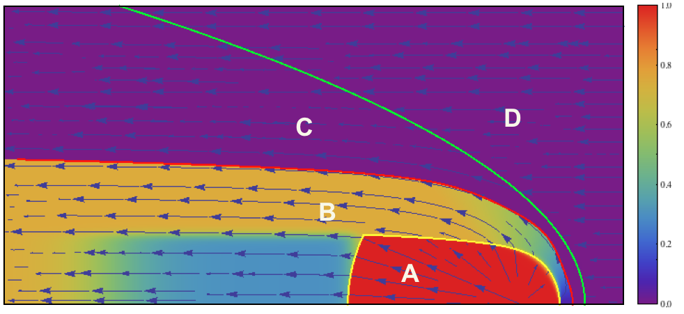
Figure 2: Upper panel: the color image represents the density structure of a bow-shock taken from an axisymmetric relativistic hydrodynamical simulation. The superimposed curves are the location of the termination shock (yellow), the contact discontinuity (red) and the forward bowshock (green) of our analytical steady state model. Middle panel: the color image represents the velocity magnitude of the bow-shock taken from the same axisymmetric relativistic hydrodynamical simulation, at the same time. Lower panel: the flow structure assumed in out model. The color map represents the magnitude of the velocity field, while the arrows indicate its direction. The colored curves are the same as in the upper panel. Labels refer to: A unshocked pulsar wind, B shocked pulsar wind, C shocked ISM material, D unshocked ISM.

However, we are here interested in developing a simplified model, capable of capturing the key properties of the flow, without all the complexity that only full fledged 3D high resolution numerical simulations can handle. We therefore chose to assume a steady state, axisymmetric laminar flow structure, representative of typical average flow conditions, as can be derived from existing simulations. Based on hydrodynamical 2D axisymmetric numerical simulations we have derived analytical formulas for the shape of the termination shock and of the forward bow-shock. The size of the various regions is scaled such that the CD along the $z-$direction is located at a unitary distance from the pulsar. This is equivalent to normalizing the lengths of the model to the stand-off distance defined as:

$$d_{o}=\sqrt{\frac{L}{4\pi c\rho_{o}V^{2}}}$$ (10)

where $L$ is the pulsar spin-down luminosity, $\rho_{o}$ is the ISM density, and $V$ is the relative speed of the pulsar with respect to the ISM. The flow is moving radially at the speed of light within the termination shock (in region A), $\boldsymbol{v}=c\boldsymbol{e}_{r}$, while matter in the outer ISM (region D) is moving with a speed $-V$ along the $z-$ axis, $\boldsymbol{v}=-V\boldsymbol{e}_{z}$. To define the direction of the flow field in both region B and C we adopt the same analytical formula. The only difference in the two regions is the velocity magnitude. The use of the same analytical formula for the flow direction, ensures that the contact discontinuity is mathematically well defined (if one had used two different prescriptions for the direction of the flow speed in region B and C, then it would have been necessary to enforce the correct matching at the supposed CD). The analytical prescription for the flow field in region B and C is chosen in order to reproduce at best the typical location of the CD (see App. A). This (together with the decision to adopt simple analytical prescriptions) implies that, at the two shocks, the jump conditions are not satisfied. This however affects the flow only locally. The magnitude of the velocity in region B and C is chosen in order to reproduce the typical trend found in numerical simulations. In region B (the one we are interested in for non-thermal emission) the velocity is seen to rise linearly, from very small values in the head, to values $\sim 0.75-0.85c$ in the tail. We therefore assume a linear trend with angular displacement from the $z-$axis. We also include the presence a slowly moving inner channel downstream of the Mach Disk. Fig. 2 illustrates the velocity field and magnitude we have adopted, to be compared with existing numerical simulations (see for example Fig. 1 of Bucciantini, Amato & Del Zanna (2005)). Despite its simplicity the flow field encapsulates all the key properties found in more sophisticated 2D axisymmetric simulations. In our simplified model we assume that the energy flux in the pulsar wind is isotropic. However numerical simulations of pulsar magnetospheres (Spitkovsky, 2006; Tchekhovskoy, Spitkovsky & Li, 2013; Tchekhovskoy, Philippov & Spitkovsky, 2016) show that the wind has likely a higher equatorial energy flux. This has consequences on the shape of the TS, which partly reflects the energy flux of the wind (Del Zanna, Amato & Bucciantini, 2004), and on the post shock flow, creating flow channels that can trigger the developement of turbulence and affect the overall variability of the system (Camus et al., 2009).

4 Magnetic Field Injection

The use of a laminar steady-state flow field ensures that each point of the BSPWN system can be associated one to one to an injection location. For the ISM the injection can be placed anywhere in region D. For the pulsar material injection can be placed at any radius in region A, where one can use standard predictions for the structure and geometry of the magnetic field in pulsar winds. In particular we set our injection boundary for the pulsar magnetic field on a sphere with radius $R_{o}=0.5d_{o}$. We are interested in modeling the non-thermal emission from region B so we assume the ISM material to be unmagnetized. In general the pulsar spin axis will be inclined by and angle $\theta_{\rm i}$ with respect to the $z-$axis, as shown in Fig. 3. The magnetic field in the pulsar wind is assumed to be purely toroidal, and symmetric with respect to the spin axis. In principle the magnetic field strength will depend on the latitude $\psi$ with respect to the spin axis. Many existing numerical models for example assume a sin-like dependence (Komissarov & Lyubarsky, 2004; Volpi et al., 2008a; Porth, Komissarov & Keppens, 2014; Olmi et al., 2015, 2016), and possibly the presence of en equatorial unmagnetized region, to account for dissipation of a striped wind.

In a cartesian reference frame centered on the pulsar with the $x-$ axis chosen such that the pulsar spin axis lays on the $x-z$ plane (Fig. 3), the magnetic field $\boldsymbol{B}_{o}$ at a point $\boldsymbol{P}_{o}=[x_{o},y_{o},z_{o}]$ in the wind will be given, in terms of cartesian components, by:

$$\boldsymbol{B}_{o}\propto\frac{F(\psi)}{r_{o}\mathcal{R}}\begin{cases}y_{o}\cos{\theta_{\rm i}}\boldsymbol{e}_{x}\\ (z_{o}\sin{\theta_{\rm i}}-x_{o}\cos{\theta_{\rm i}})\boldsymbol{e}_{y}\\ -y_{o}\sin{\theta_{\rm i}}\boldsymbol{e}_{z}\end{cases}$$ (11)

where $r_{o}=\sqrt{x_{o}^{2}+y_{o}^{2}+z_{o}^{2}}$, $\mathcal{R}^{2}=y_{o}^{2}+x_{o}^{2}\cos^{2}{\theta_{\rm i}}+z_{o}^{2}\sin^{2}{\theta_{\rm i}}-x_{o}z_{o}\sin{2\theta_{\rm i}}$. $\psi$ represents the angular distance of a point from the pulsar spin axis, $\cos{\psi}=[x_{o}\cos{\theta_{\rm i}}+z_{o}\sin{\theta_{\rm i}}]/r_{o}$, and $F(\psi)$ parametrizes the latitudinal dependence of the magnetic field strength.

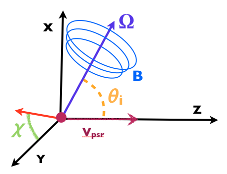
Figure 3: Geometry of the magnetic field in the pulsar wind. The $z-$axis is aligned to the pulsar speed $\boldsymbol{v}_{\rm psr}$ with respect to the ISM (or equivalently the ISM speed in the reference frame of the pulsar). $\boldsymbol{\Omega}$ is the pulsar spin axis, around which the pulsar wind magnetic field $\boldsymbol{B}$ is wound-up, which lays in the $x-z$ plane and is inclined $\theta_{\rm i}$ with respect to the $z-$ axis. $\chi$ indicates the inclination angle of the direction pointing toward the observer, which is assumed to be perpendicular to the $z-$axis (the pulsar velocity is in the plane of the sky).

5 Results

We present here the results of a serie of models done using various inclinations of the pulsar spin axis $\theta_{\rm i}$ and various orientation $\chi$ of the observer. We are mostly interested in modeling the magnetic field structure and simulating the non-thermal radio emission, including polarization, in oder to obtain an understanding of the basic features one might expect to see in these systems. In the following, in line with the standard assumptions on the magnetic field distribution in pulsar winds, we assume $F(\psi)=\sin{\psi}$, unless otherwise stated. Moreover we assume that the velocity field is independent on the magnetic field strength. This is formally correct only as long as the magnetic field energy is sub-equipartition.

5.1 Magnetic surfaces

In a steady state laminar flow, magnetic loops, coming from the wind, will retain their coherence and trace, during their evolution, the location of the magnetic surface to which they belong. A set of nested magnetic surfaces will then arise as a consequence of the flow. In Fig. 4 we show the shape of magnetic field surfaces, for various inclinations of the pulsar spin axis. In the co-aligned case, $\theta_{\rm i}=0$, the magnetic surfaces are axisymmetric, while for other inclinations, a magnetic chimney forms on the front side, with magnetic loops strongly stretched, and piled-up. It is evident that the flow structure tends to concentrate the magnetic surfaces toward the contact discontinuity. This effect was already observed in earlier axisymmetric simulations (Bucciantini, Amato & Del Zanna, 2005). This will lead to the formation of a magnetopause, where the magnetic field strength can rise above equipartition. Magnetopauses are a common feature in magnetically confined flows, and are sites of possible violent reconnection and dissipation (Mozer et al., 1978; Galeev, 1983; Alexeev & Kalegaev, 1995). In the axisymmetric case, the structure of the magnetic surfaces ensures that there will be no polarity inversion close to the CD, suppressing in principle reconnection events. On the contrary, in the magnetic chimney that form for other values of $\theta_{\rm i}$, field lines of different polarity are brought close together, in principle creating the conditions for fast reconnection and dissipation. It is then possible that the magnetic chimney behaves as a highly dissipative structure. On the other hand, the magnetic surfaces are quite open on the back side, downstream of the Mach Disk, suggesting that low values of the magnetic field might be characteristic of the inner flow channel. Indeed the backward magnetic chimney shows no sign of stretching or compression.

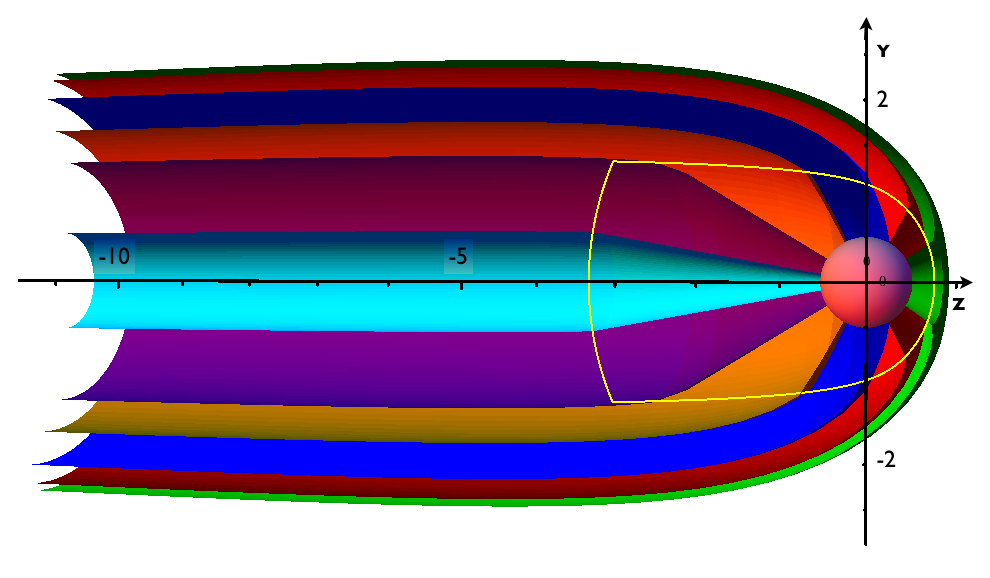
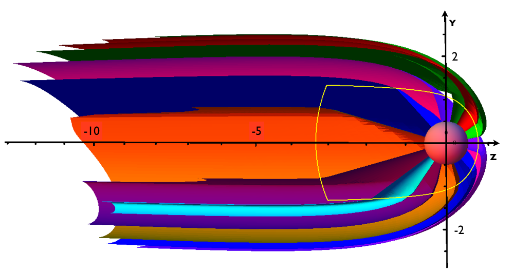
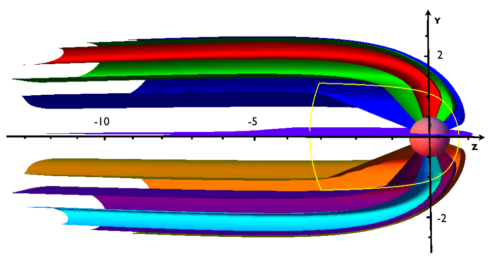
Figure 4: Sections of magnetic field surfaces, for various inclination of the pulsar spin axis. From top to bottom $\theta_{\rm i}=0,45^{\circ},90^{\circ}$. Magnetic surfaces have been selected to sample as best as possible the distribution of magnetic loops in the nebula. The yellow curve is a section of the pulsar wind TS.

5.2 Emission maps

Let us recall that we are interested in radio emission, and radio emitting particles have synchrotron lifetime longer that the flow time in the nebula. Following Del Zanna et al. (2006), if we assume that the emitting pairs are distributed in energy $\epsilon$, according to a power-law $n(\epsilon)=K\epsilon^{-(2\alpha+1)}$, then their local synchrotron emissivity at frequency $\nu$, toward the observer will be:

$$j(\nu,\boldsymbol{n})=C|\boldsymbol{B}^{\prime}\times\boldsymbol{n}^{\prime}|^{\alpha+1}D^{\alpha+2}\nu^{-\alpha}$$ (12)

where $\boldsymbol{B}^{\prime}$ and $\boldsymbol{n}^{\prime}$ are the magnetic field and the observer direction measured in the frame comoving with the flow, and $C$ is a normalization constant dependent on $K$. $D$ is the Doppler boosting coefficient

$$D=\frac{\sqrt{1-\beta^{2}}}{1-\boldsymbol{\beta}\cdot\boldsymbol{n}}=\frac{1}{\gamma(1-\boldsymbol{\beta}\cdot\boldsymbol{n})}$$ (13)

where $\gamma$ is the Lorentz factor of the flow, $\boldsymbol{\beta}$ and $\boldsymbol{n}$ respectively the flow speed normalized to $c$ and the observer direction, both measured in the observer frame. Now, in terms of quantities measured in the observer frame (unprimed), one has

$$|\boldsymbol{B}^{\prime}\times\boldsymbol{n}^{\prime}|=\frac{1}{\gamma}\sqrt{B^{2}-D^{2}(\boldsymbol{B}\cdot\boldsymbol{n})^{2}+2\gamma D(\boldsymbol{B}\cdot\boldsymbol{n})(\boldsymbol{B}\cdot\boldsymbol{\beta})}$$ (14)

One can also compute the polarization angle $\xi$, that enters into the definition of the Stoke’s parameters $Q$ and $U$. Choosing a Cartesian reference frame with the observer in the $X$ direction, one finds

$$\cos{2\xi}=\frac{q_{Y}^{2}-q_{Z}^{2}}{q_{Y}^{2}+q_{Z}^{2}},\quad\quad\sin{2\xi}=-\frac{q_{Y}q_{Z}}{q_{Y}^{2}+q_{Z}^{2}},$$ (15)

where

$$q_{Y}=(1-\beta_{X})B_{Y}+\beta_{Y}B_{X}\quad\quad q_{Z}=(1-\beta_{X})B_{Z}+\beta_{Z}B_{X}$$ (16)

In principle the local emissivity also depends on the local density of emitting particles ($K$). This, as well as the power-law index $\alpha$, will in principle be a function of the injection location along the TS (different locations being characterized by different physical conditions in terms of wind magnetization, presence of a striped component, wind Lorentz factor etc….). In our Lagrangian formalism, we can trace the injection location along the TS for each fluid element in the BSPWN. However, given that there is no consensus on how particles are accelerated at a relativistic termination shock, that current models provide little hint on possible injection recipes, and that observations do not have enough resolution to assess possible variations of the spectral index, one can assume that the particle power-law index $\alpha$ is uniform in the nebula. Furthermore, we also assume, for simplicity, that the normalization constant $K$ is also uniform. This is equivalent to the assumption of a uniform density for the emitting particles. Given that the divergence of the flow field we use in our model is small (at most a factor 2 between the head and the tail), this is roughly equivalent to the assumption of uniform injection at the TS. In all of the following, to limit the possible parameter space, we consider only the case where the observer’s direction is perpendicular to the pulsar velocity (the pulsar velocity is in the plnae of the sky). In this case, the observer direction is parametrized only by the viewing angle $\chi$ (see Fig. 3).

In the axisymmetric case, $\theta_{\rm i}=0^{\circ}$, the emission pattern is independent of the viewing angle $\chi$. In Fig. 5 we show the expected synchrotron intensity for a flat radio spectrum, $\alpha=0$, and for three different choices of magnetic field distribution in the wind. Given that we are interested in the polarimetric signatures associated to the magnetic field geometry, we opted for a flat spectrum in accordance with the typical radio spectral indexes of PWNe (Gaensler & Slane, 2006), and radio bow-shocks (Predehl & Kulkarni, 1995; Ng et al., 2010, 2012). In the same figure the polarization pattern is also shown. In all cases the intensity peaks in the very head. This is due to Doppler boosting, given that it is the only location in the nebula where the flow velocity points toward the observer. What distinguishes the various cases, is how narrow the intensity peak is. Obviously, this depends on the strength of the magnetic field at the pole, with respect to the one at the equator (the level of magnetic anisotropy in the wind), which is maximal for $F(\psi)=\sin{(\psi)}$, and minimal for $F(\psi)=const$. The other interesting common feature, also connected to Doppler boosting, is the high brightness region located between $Z=-8$ and $Z=-3$ that corresponds to the slow inner channel that forms downstream of the Mach Disk. Being the velocity in this channel smaller than in the surrounding region, the emission is less de-boosted. The brightness contrast again depends on the magnetic anisotropy, being maximal for $F(\psi)=const$. In general, in the case $F(\psi)=\sin{(\psi)}$, the brightness contrast among the various features, is so attenuated that on average the surface brightness looks more uniform, in the volume of the nebula.

In the same Fig. 5, we also show for the same configurations the polarization angle (orthogonal to the electric field). Given that the magnetic field is, in the axisymmetric case, always orthogonal to the pulsar kick velocity, one would have naively expected the polarization to be everywhere orthogonal to the $Z$-axis. However, it is well known that relativistic motion leads to polarization angle swing (Bjornsson, 1982; Qian & Zhang, 2003; Bucciantini et al., 2005, 2017), and this becomes dominant in the outer fast flow channel. In Fig. 6 we show the polarized intensity. The same considerations discussed previously for the level of brightness contrast, and its dependence on the magnetic anisotropy of the wind, apply also for polarized emission. The polarization angle swing leads to a depolarized region between the inner slow channel and the CD. Interestingly the inner slow channel is more evident in polarized light than in total light. The polarized intensity in the inner channel ranges from 40% to 60% of the maximum total intensity, while the bulk of the nebula has in general a much lower level of polarization, less than 30% of the maximum. The polarized fraction for the case $F(\psi)=\sin{(\psi)}$ is shown in Fig. 7. The polarized fraction reaches the theoretical maximum on axis, where, because of the symmetry of the configuration, there are no depolarization effects. It then drops to zero as one approaches the region where the relativistic polarization angle swing appears, and then rises again toward the CD, where however the luminosity vanishes. The other cases have a similar pattern.

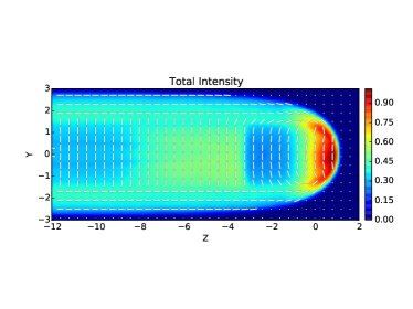
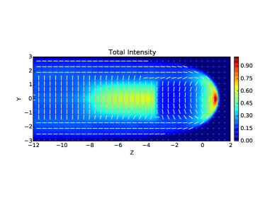
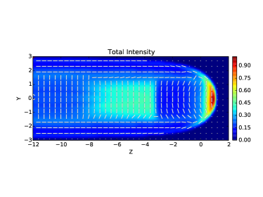
Figure 5: Total synchrotron intensity in the completely axysymmetric case $\theta_{\rm i}=0$ for different choices of the magnetic field distribution in the wind: upper panel $F(\psi)=\sin{(\psi)}$, middle panel $F(\psi)=const$, lower panel $F(\psi)=\sin{(\psi)}\tanh{(\Pi/2-\psi)}$ (representative of a large striped wind). Intensity is normalized to the maximum. Dashes indicate the orientation of the polarization vector (not its amplitude). The pulsar is located in $Y=0$ $Z=0$.

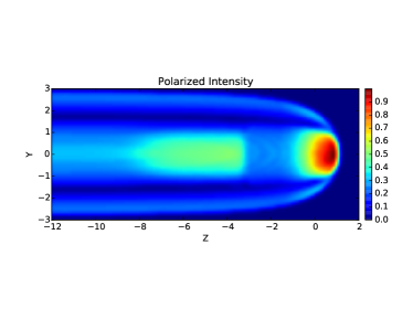
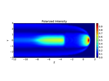
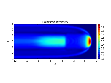
Figure 6: Same as Fig. 5 but for polarized intensity. Maps are normalized to the maximum of the total intensity.

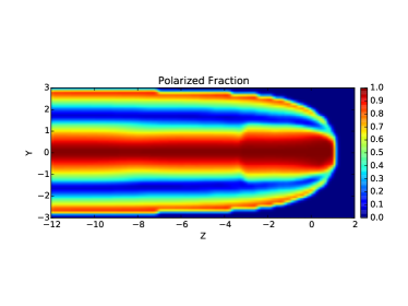
Figure 7: Polarized fraction for the case $\theta_{\rm i}=0$, $F(\psi)=\sin{(\psi)}$.

In Fig.s 8 and 9 we show the total surface brightness, polarization angle and polarized intensity, for the fully orthogonal case $\theta_{\rm i}=90^{\circ}$. We limit our model to the canonical $F(\psi)=\sin{(\psi)}$ profile for the magnetic field distribution in the wind, and investigate the appearance of the nebula at three different viewing angles $\chi=0,45$ and $90$ degrees. For $\theta_{\rm i}=90^{\circ}$ the system is symmetric with respect to the direction transverse to the $Z$-axis both for $\chi=0^{\circ}$ and $\chi=90^{\circ}$. With respect to the axisymmetric case $\theta_{\rm i}=0^{\circ}$ we note immediately that the region corresponding to the inner slow channel downstream of the Mach Disk, is brighter, while the outer parts of the nebula are far weaker. The brightness profile in the head is now strongly dependent of the viewing orientation, becoming very arcuate for $\chi=90^{\circ}$, while at intermediate viewing angles it shows a clear asymmetry, as expected. In practice we are observing how the emission from the magnetic chimney changes, depending on orientation. Even the orientation of the polarization angle is as expected. Interestingly for $\chi=90^{\circ}$ the observed polarization angle follows the shape of the CD in the head. In this case, the inclination of the polarization in the tail maps the relative angle between the observer and the pulsar spin axis. On the other hand major differences are evident in the map of polarized intensity. For $\chi=0^{\circ}$ the polarized intensity in the region corresponding to the slow inner flow channel can reach values up to 70% of the total brightens maximum, significantly larger than in the axisymmetric $\theta_{\rm i}=0^{\circ}$ case, and even in the asymptotic tail polarizations of 40% of the maximum are possible. In this case the pattern of polarized fraction is similar (because of symmetry) to the one shown in Fig. 7. For other viewing angles instead, the polarized intensity can be quite smaller. For $\chi=45^{\circ}$ the inner slow channel appears weak in polarized light. For $\chi=90^{\circ}$ the polarized intensity in the inner flow channel is still high (comparable to the axysymmetric case). Note that the regions with high polarized intensity located in the tail at $Y=\pm 1.3$ are due to the local strong shear between the inner slow channel and the outer fast flow, that leads to a strong distortion of the local magnetic field. In terms of polarized fraction the results for $\chi=45^{\circ}$ and $\chi=90^{\circ}$ are shown in Fig. 10. The tail tends to become progressively more polarized, and at $\chi=90^{\circ}$ results uniformly in excess of 70% of the theoretical maximum.

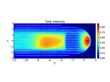
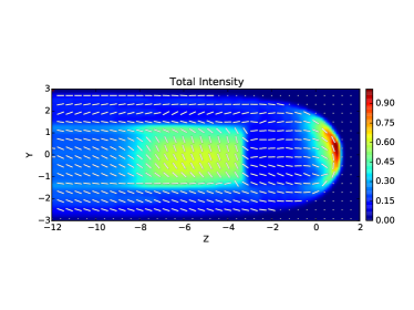
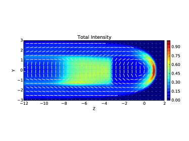
Figure 8: Total synchrotron intensity in the completely orthogonal case $\theta_{\rm i}=90^{\circ}$ with $F(\psi)=\sin{(\psi)}$, but for different choices of the observer viewing angle: upper panel $\chi=0^{\circ}$, middle panel $\chi=45^{\circ}$, lower panel $\chi=90^{\circ}$. Intensity is normalized to the maximum. Dashes indicate the orientation of the polarization vector (not its amplitude). The pulsar is located in $Y=0$ $Z=0$.

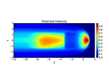
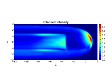
Figure 9: Same as Fig. 8 but for polarized intensity. Maps are normalized to the maximum of the total intensity.

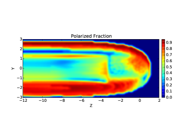
Figure 10: Polarized fraction for the case $\theta_{\rm i}=0$, $F(\psi)=\sin{(\psi)}$, and two different values of the viewing angle: upper panel $\chi=45^{\circ}$, lower panel $\chi=0^{\circ}$.

In Fig.s 11 and 12 we show the total surface brightness, polarization angle and polarized intensity, for the intermediate case $\theta_{\rm i}=45^{\circ}$. We limit again our model to the canonical $F(\psi)=\sin{(\psi)}$ profile for the magnetic field distribution in the wind, and investigate the appearance of the nebula at five different viewing angles $\chi=0,45,90,135,180$ degrees. In this case, in fact, the presence of an inclined magnetic chimney defines a privileged orientation breaking the up-down symmetry of the orthogonal case. It is evident that the major differences due to the observer inclination $\chi$ are in the brightness profile of the head that changes from arch-like to more concentrated. It is also evident that the level of asymmetry is maximal when the magnetic chimney points toward the observer than when it points away. Also the polarization angle experiences a similar change from orthogonal to quasi-parallel to the $Z$-axis. Looking at the polarized intensity we see that, in the tail the region corresponding to the inner slow flow channel in the cases $\chi=0^{\circ}$ and $\chi=180^{\circ}$, it shows a high level of polarized intensity $\sim 60$% of the total brightness maximum, less than in the orthogonal case but higher that for the completely axisymmetric case. However, for other inclinations the polarized intensity drops substantially and the tails looks almost uniform in polarized emission for $\chi=90^{\circ}$. In terms of polarized fraction we find that for $\chi=0^{\circ}$ and $\chi=180^{\circ}$ the polarized fraction on axis reaches its theoretical maximum (as expected given that at this observer inclination there are no depolarization effects on axis). It also reaches values close to 70-80% of the theoretical maximum close to the CD. For $\chi=90^{\circ}$ instead the polarized fraction in the tail appears uniform at about 50-60% of the theoretical maximum.

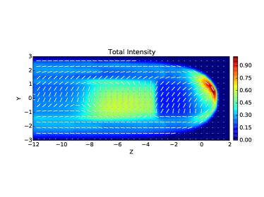
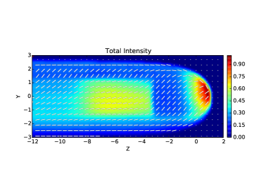
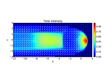
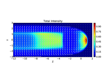
Figure 11: Total synchrotron intensity in the inclined case $\theta_{\rm i}=45^{\circ}$ with $F(\psi)=\sin{(\psi)}$, but for different choices of the observer viewing angle: from the upper panel to the lower one $\chi=90,45,0,-45,-90$ degrees. Intensity is normalized to the maximum. Dashes indicate the orientation of the polarization vector (not its amplitude). The pulsar is located in $Y=0$ $Z=0$.

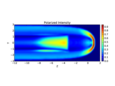
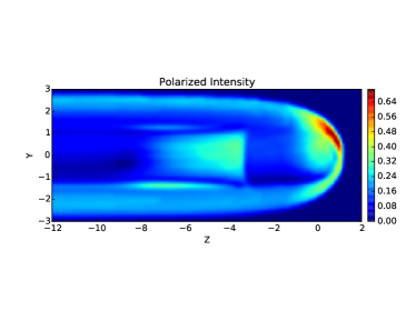
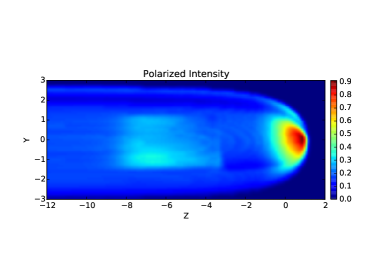
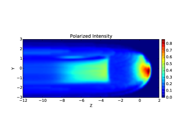
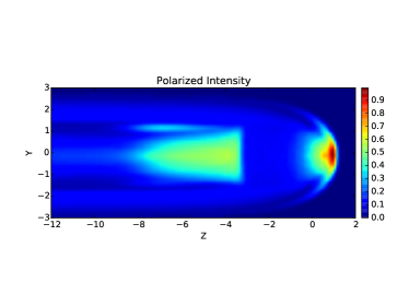
Figure 12: Same as Fig. 11 but for polarized intensity. Maps are normalized to the maximum of the total intensity.

5.3 The role of the spectral index

We briefly illustrate here how the emission maps change, varying the spectral index $\alpha$. Observations suggest that the radio spectral index should be quite flat. In Fig. 13 we show the total intensity map corresponding to the case $\alpha=0.6$, for a few selected geometries. It is immediately evindent that, a steeper spectral index, produces maps of total intensity (the same hold for the polarized intensity), where the contrast between brighter and fainter regions is enhanced, and the presence of a brighter region in the tail, corresponding to the slow inner channel, is much less evident. The reason for this behaviour can be understood by looking at Eq. 12, where is it evident that a higher value of $\alpha$ will increase the emissivity toward the observer from the regions of stronger field (the head) and the regions of higher Doppler boosting (again in the head where the flow points toward the observer), with respect to the tail. The first panel of Fig. 13, shows a map in a configuration analogous to the low magnetization case of Bucciantini, Amato & Del Zanna (2005), which also shows a stronger emission in the head, with no evidence for a brighter region in the tail corresponding to the slow moving channel. However a direct comparison is not possible, because Bucciantini, Amato & Del Zanna (2005), being mostly interested in the X-ray properties, adopt a pressure normalization in the emissivity, and include the effect of synchrotron cooling. These two extra terms enhance even more the head to tail brightness ratio. Interestingly the choice of spectral index does not affect the polarization structure.

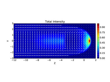
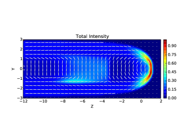
Figure 13: Total intensity maps for a spectral index $\alpha=0.6$. Upper panel: completely axisymmetric case $\theta_{\rm i}=0$, with $F(\psi)=const$ (see middle panel of Fig. 5 for comparison). Middle panel: inclined case $\theta_{\rm i}=45^{\circ}$ with $F(\psi)=\sin{(\psi)}$ and $\chi=90$ ( see top panel of Fig. 11 for comparison). Bottom panel: inclined case $\theta_{\rm i}=45^{\circ}$ with $F(\psi)=\sin{(\psi)}$ and $\chi=45$ ( see second panel of Fig. 11 for comparison).

6 Conclusions

We have introduced here a method based on Lagrangian tracers to compute the structure and geometry of the magnetic field for a given velocity field in 3D, and we have applied it to compute the structure of the magnetic field expected inside a Bow Shock Pulsar Wind Nebula. This approach allowed us to compute the full magnetic structure of the nebula on a single CPU in just a few hours as opposed to full multidimensional numerical models that require hundreds of hours on large scale multiprocessor machines. A simple analytical steady-state laminar flow pattern has been adopted to describe the properties of the flow of the material injected by the pulsar, and responsible for the non-thermal emission that is observer. Despite the simplicity of this assumption we have shown that a rich morphology in terms of radio emission maps and polarized properties can arise due to the combination of different inclinations of the pulsar spin axis, different distributions of the magnetic field in the pulsar wind, and different orientations of the observer. We caution the reader however, that more complex flow structures can arise, if an energy flux anisotropy of the wind is assumed, as suggested by magnetospheric moldels of pulsars.

We have shown that major asymmetries due to the orientation of the spin axis or the observer are preferentially confined in the very head, where the emission pattern can change substantially, while the region of the tail shows generally a quite similar appearance, with major differences being related to the intensity of the slow flow channel that is expected to arise downstream of the Mach Disk. This shows that bright regions downstream of the termination shock are likely associated to slowly moving material (bright spots in the tail of known radio BSPWNe could then be associated to shocks that slow down the flow). Given that the laminar assumption, that for simplicity we have introduced, might not be correct in the presence of strong shear, at the CD, one can in principle use the brightness ratio of the tail vs the head as a proxy for the flow speed. Nebulae that show no major brightness contrast are likely to be characterized by slow flow speed in the tail, that could be the consequence either of shear and turbulence developed at the CD or of mixing with the denser and slower ISM material. However, we have also show that the brightness contrast is strongly dependent on the spectal index: a steeper spectrum enhancing the head to tail brightness ratio. So one should take care in interpreting observational results. We have also investigated the polarization properties of the BSPWNe, and verified that with a good approximation the orientation of the polarization in the tail can be used as a good proxy for the orientation of the magnetic axis, with polarization pattern that ranges from aligned to the pulsar speed to orthogonal. The polarized fraction is found to be in general quite high, with depolarization being limited only to certain specific configurations. This could also be used to constrain the level of turbulence in observed systems, by comparing the observed polarized fraction with the expectation of a fully laminar model. For example the Frying Pan G315.78-0.23 (Ng et al., 2012) has a very ordered magnetic field aligned with the tail (as in the upper panel of Fig. 8), with a polarized fraction of 40-50%, and extending for several parsecs. Using the subgrid model by Bandiera & Petruk (2016) recently applied to PWNe (Bucciantini et al., 2017; Bucciantini & Olmi, 2018), we can estimate a typical turbulence with $\delta B/B\sim 0.3$. On the other hand low polarization systems like the Mouse G359.23-0.82 (Yusef-Zadeh & Gaensler, 2005), with polarized fraction below 10% are likely characterized by strong turbulence, in part already evident in the rapid change of polarization pattern. Intermediate cases with polarization $\sim$30% (Ng et al., 2010) on the other hand suggest a turbulence with $\delta B/B\sim 1$.

Our model does not include dissipation, however it is evident from the shape of the magnetic surfaces, that the magnetic chimney can be strongly compressed and distorted in the head of a BSPWN, leading to the formation of a region where the current density is high. This region might be prone to reconnection and dissipation, leading to a local heating and acceleration of particles. We cannot exclude that bright thin non-symmetric features might form close to the CD. This could be the case of the hard tails observed for example in Geminga (Posselt et al., 2017).

In this paper we have limited our study to the emission properties of the BSPWNe. However the method we have introduced can be used to model also the structure of the magnetic field of the ISM. We plan in the future to extend this model to include the ambient magnetic field, in order to evaluate which configurations, in terms of relative orientation of the pulsar spin axis and ISM magnetic field, could be promising for reconnection of the internal and external magnetic field. This process has been invoked (Bandiera, 2008) in order to explain bright X-ray features observed in the Guitar and Lighthouse nebulae (Hui & Becker, 2007; Pavan et al., 2014) that emerge almost orthogonally from the head of the bow shock, far beyond the supposed position of the CD. The general idea is that particles can diffuse from the BSPWN to the ISM via loci at the CD of preferential reconnection.

Appendix A Flow field

We provide here the analytical expression for the direction of the velocity field used in region B and C of the nebula, in a cylindrical reference frame $(R,Z)$. with the $Z$-axis pointing along the pulsar speed. The pulsar speed into the ISM has norm $V$.

$$\frac{v_{Z}}{v} =\frac{\frac{Z}{\left(R^{2}+Z^{2}\right)^{3/2}}-\frac{V}{c}}{\sqrt{\left(\frac{Z}{\left(R^{2}+Z^{2}\right)^{3/2}}-\frac{V}{c}\right)^{2}+\frac{\left(R^{3/10}+1\right)^{2}R^{2}}{\left(R^{2}+Z^{2}\right)^{3}}}}$$ (17)

$$\frac{v_{R}}{v} =\frac{\left(R^{3/10}+1\right)R}{\left(R^{2}+Z^{2}\right)^{3/2}\sqrt{\left(\frac{Z}{\left(R^{2}+Z^{2}\right)^{3/2}}-\frac{V}{c}\right)^{2}+\frac{\left(R^{3/10}+1\right)^{2}R^{2}}{\left(R^{2}+Z^{2}\right)^{3}}}}$$ (18)

References

- Adriani et al. (2009) Adriani O. et al., 2009, Nature, 458, 607
- Adriani et al. (2013) —, 2013, Soviet Journal of Experimental and Theoretical Physics Letters, 96, 621
- Aguilar et al. (2013) Aguilar M. et al., 2013, Physical Review Letters, 110, 141102
- Alexeev & Kalegaev (1995) Alexeev I. I., Kalegaev V. V., 1995, J. Geophys. Res., 100, 19267
- Arons & Scharlemann (1979) Arons J., Scharlemann E. T., 1979, ApJ, 231, 854
- Arzoumanian, Chernoff & Cordes (2002) Arzoumanian Z., Chernoff D. F., Cordes J. M., 2002, ApJ, 568, 289
- Arzoumanian et al. (2004) Arzoumanian Z., Cordes J., Van Buren D., Corcoran M., Safi-Harb S., Petre R., 2004, in Bulletin of the American Astronomical Society, Vol. 36, AAS/High Energy Astrophysics Division #8, p. 951
- Bandiera (1993) Bandiera R., 1993, A&A, 276, 648
- Bandiera (2008) —, 2008, A&A, 490, L3
- Bandiera & Petruk (2016) Bandiera R., Petruk O., 2016, MNRAS, 459, 178
- Begelman & Li (1992) Begelman M. C., Li Z.-Y., 1992, ApJ, 397, 187
- Bell et al. (1995) Bell J. F., Bailes M., Manchester R. N., Weisberg J. M., Lyne A. G., 1995, ApJLett, 440, L81
- Berera & Ho (2018) Berera A., Ho R. D. J. G., 2018, Physical Review Letters, 120, 024101
- Biferale et al. (2005) Biferale L., Boffetta G., Celani A., Devenish B. J., Lanotte A., Toschi F., 2005, Physics of Fluids, 17, 115101
- Bjornsson (1982) Bjornsson C.-I., 1982, ApJ, 260, 855
- Blasi & Amato (2011) Blasi P., Amato E., 2011, Astrophysics and Space Science Proceedings, 21, 624
- Bogovalov (1999) Bogovalov S. V., 1999, A&A, 349, 1017
- Bogovalov et al. (2005) Bogovalov S. V., Chechetkin V. M., Koldoba A. V., Ustyugova G. V., 2005, MNRAS, 358, 705
- Borkowski et al. (2013) Borkowski K. J., Reynolds S. P., Hwang U., Green D. A., Petre R., Krishnamurthy K., Willett R., 2013, ApJLett, 771, L9
- Brownsberger & Romani (2014) Brownsberger S., Romani R. W., 2014, ApJ, 784, 154
- Bucciantini (2002a) Bucciantini N., 2002a, in Astronomical Society of the Pacific Conference Series, Vol. 271, Neutron Stars in Supernova Remnants, P. O. Slane & B. M. Gaensler, ed., pp. 109–+
- Bucciantini (2002b) —, 2002b, A&A, 387, 1066
- Bucciantini (2002c) —, 2002c, A&A, 393, 629
- Bucciantini (2008) —, 2008, Advances in Space Research, 41, 491
- Bucciantini, Amato & Del Zanna (2005) Bucciantini N., Amato E., Del Zanna L., 2005, A&A, 434, 189
- Bucciantini & Bandiera (2001) Bucciantini N., Bandiera R., 2001, A&A, 375, 1032
- Bucciantini et al. (2017) Bucciantini N., Bandiera R., Olmi B., Del Zanna L., 2017, MNRAS, 470, 4066
- Bucciantini et al. (2005) Bucciantini N., del Zanna L., Amato E., Volpi D., 2005, A&A, 443, 519
- Bucciantini & Olmi (2018) Bucciantini N., Olmi B., 2018, MNRAS, 475, 822
- Camus et al. (2009) Camus N. F., Komissarov S. S., Bucciantini N., Hughes P. A., 2009, MNRAS, 400, 1241
- Cerutti & Philippov (2017) Cerutti B., Philippov A. A., 2017, A&A, 607, A134
- Chatterjee et al. (2005) Chatterjee S., Gaensler B. M., Vigelius M., Cordes J. M., Arzoumanian Z., Stappers B., Ghavamian P., Melatos A., 2005, in Bulletin of the American Astronomical Society, Vol. 37, American Astronomical Society Meeting Abstracts, p. 1470
- Chevalier, Kirshner & Raymond (1980) Chevalier R. A., Kirshner R. P., Raymond J. C., 1980, ApJ, 235, 186
- Cioffi, McKee & Bertschinger (1988) Cioffi D. F., McKee C. F., Bertschinger E., 1988, ApJ, 334, 252
- Cordes & Chernoff (1998) Cordes J. M., Chernoff D. F., 1998, ApJ, 505, 315
- Cordes, Romani & Lundgren (1993) Cordes J. M., Romani R. W., Lundgren S. C., 1993, Nature, 362, 133
- De Luca et al. (2011) De Luca A. et al., 2011, ApJ, 733, 104
- Del Zanna, Amato & Bucciantini (2004) Del Zanna L., Amato E., Bucciantini N., 2004, A&A, 421, 1063
- Del Zanna & Olmi (2017) Del Zanna L., Olmi B., 2017, in Astrophysics and Space Science Library, Vol. 446, Modelling Pulsar Wind Nebulae, Torres D. F., ed., p. 215
- Del Zanna et al. (2006) Del Zanna L., Volpi D., Amato E., Bucciantini N., 2006, A&A, 453, 621
- DeLaney & Rudnick (2003) DeLaney T., Rudnick L., 2003, ApJ, 589, 818
- Gaensler (2005) Gaensler B. M., 2005, Advances in Space Research, 35, 1116
- Gaensler & Slane (2006) Gaensler B. M., Slane P. O., 2006, ARA&A, 44, 17
- Gaensler et al. (2004) Gaensler B. M., van der Swaluw E., Camilo F., Kaspi V. M., Baganoff F. K., Yusef-Zadeh F., Manchester R. N., 2004, ApJ, 616, 383
- Galeev (1983) Galeev A. A., 1983, Space Sci. Rev., 34, 213
- Ghavamian et al. (2001) Ghavamian P., Raymond J., Smith R. C., Hartigan P., 2001, ApJ, 547, 995
- Gold (1968) Gold T., 1968, Nature, 218, 731
- Goldreich & Julian (1969) Goldreich P., Julian W. H., 1969, ApJ, 157, 869
- Hales et al. (2009) Hales C. A., Gaensler B. M., Chatterjee S., van der Swaluw E., Camilo F., 2009, ApJ, 706, 1316
- Hester (2008) Hester J. J., 2008, ARA&A, 46, 127
- Hester, Raymond & Blair (1994) Hester J. J., Raymond J. C., Blair W. P., 1994, ApJ, 420, 721
- Hibschman & Arons (2001) Hibschman J. A., Arons J., 2001, ApJ, 554, 624
- Hooper, Blasi & Dario Serpico (2009) Hooper D., Blasi P., Dario Serpico P., 2009, JCAP, 1, 025
- Hughes (1999) Hughes J. P., 1999, ApJ, 527, 298
- Hughes (2000) —, 2000, ApJLett, 545, L53
- Hui & Becker (2007) Hui C. Y., Becker W., 2007, A&A, 467, 1209
- Hui et al. (2012) Hui C. Y., Huang R. H. H., Trepl L., Tetzlaff N., Takata J., Wu E. M. H., Cheng K. S., 2012, ApJ, 747, 74
- Jakobsen et al. (2014) Jakobsen S. J., Tomsick J. A., Watson D., Gotthelf E. V., Kaspi V. M., 2014, ApJ, 787, 129
- Johnston et al. (2005) Johnston S., Hobbs G., Vigeland S., Kramer M., Weisberg J. M., Lyne A. G., 2005, MNRAS, 364, 1397
- Johnston et al. (2007) Johnston S., Kramer M., Karastergiou A., Hobbs G., Ord S., Wallman J., 2007, MNRAS, 381, 1625
- Jones, Stappers & Gaensler (2002) Jones D. H., Stappers B. W., Gaensler B. M., 2002, A&A, 389, L1
- Kargaltsev et al. (2008) Kargaltsev O., Misanovic Z., Pavlov G. G., Wong J. A., Garmire G. P., 2008, ApJ, 684, 542
- Kargaltsev et al. (2017) Kargaltsev O., Pavlov G. G., Klingler N., Rangelov B., 2017, Journal of Plasma Physics, 83, 635830501
- Kennel & Coroniti (1984a) Kennel C. F., Coroniti F. V., 1984a, ApJ, 283, 694
- Kennel & Coroniti (1984b) —, 1984b, ApJ, 283, 710
- Kirk & Skjæraasen (2003) Kirk J. G., Skjæraasen O., 2003, ApJ, 591, 366
- Klingler et al. (2016) Klingler N. et al., 2016, ApJ, 833, 253
- Komissarov (2013) Komissarov S. S., 2013, MNRAS, 428, 2459
- Komissarov & Lyubarsky (2004) Komissarov S. S., Lyubarsky Y. E., 2004, MNRAS, 349, 779
- Kulkarni & Hester (1988) Kulkarni S. R., Hester J. J., 1988, Nature, 335, 801
- Leahy, Green & Tian (2014) Leahy D., Green K., Tian W., 2014, MNRAS, 438, 1813
- Li, Lu & Li (2005) Li X. H., Lu F. J., Li T. P., 2005, ApJ, 628, 931
- Marelli et al. (2013) Marelli M. et al., 2013, ApJ, 765, 36
- Melatos (1998) Melatos A., 1998, Mem. SAIt, 69, 1009
- Michel (1973) Michel F. C., 1973, ApJ, 180, 207
- Misanovic, Pavlov & Garmire (2008) Misanovic Z., Pavlov G. G., Garmire G. P., 2008, ApJ, 685, 1129
- Mochol (2017) Mochol I., 2017, in Astrophysics and Space Science Library, Vol. 446, Modelling Pulsar Wind Nebulae, Torres D. F., ed., p. 135
- Morlino, Lyutikov & Vorster (2015) Morlino G., Lyutikov M., Vorster M., 2015, MNRAS, 454, 3886
- Mozer et al. (1978) Mozer F. S., Torbert R. B., Fahleson U. V., Falthammar C.-G., Gonfalone A., Pedersen A., 1978, Space Sci. Rev., 22, 791
- Ng et al. (2012) Ng C.-Y., Bucciantini N., Gaensler B. M., Camilo F., Chatterjee S., Bouchard A., 2012, ApJ, 746, 105
- Ng et al. (2009) Ng C. Y. et al., 2009, in Bulletin of the American Astronomical Society, Vol. 41, American Astronomical Society Meeting Abstracts #213, p. 307
- Ng et al. (2010) Ng C.-Y., Gaensler B. M., Chatterjee S., Johnston S., 2010, ApJ, 712, 596
- Ng & Romani (2007) Ng C.-Y., Romani R. W., 2007, ApJ, 660, 1357
- Noutsos et al. (2012) Noutsos A., Kramer M., Carr P., Johnston S., 2012, MNRAS, 423, 2736
- Noutsos et al. (2013) Noutsos A., Schnitzeler D. H. F. M., Keane E. F., Kramer M., Johnston S., 2013, MNRAS, 430, 2281
- Olmi et al. (2014) Olmi B., Del Zanna L., Amato E., Bandiera R., Bucciantini N., 2014, MNRAS, 438, 1518
- Olmi et al. (2015) Olmi B., Del Zanna L., Amato E., Bucciantini N., 2015, MNRAS, 449, 3149
- Olmi et al. (2016) Olmi B., Del Zanna L., Amato E., Bucciantini N., Mignone A., 2016, Journal of Plasma Physics, 82, 635820601
- Pacini (1967) Pacini F., 1967, Nature, 216, 567
- Pavan et al. (2014) Pavan L. et al., 2014, A&A, 562, A122
- Pétri & Lyubarsky (2007) Pétri J., Lyubarsky Y., 2007, A&A, 473, 683
- Porth, Komissarov & Keppens (2014) Porth O., Komissarov S. S., Keppens R., 2014, MNRAS, 438, 278
- Posselt et al. (2017) Posselt B. et al., 2017, ApJ, 835, 66
- Predehl & Kulkarni (1995) Predehl P., Kulkarni S. R., 1995, A&A, 294, L29
- Price (2011) Price D. J., 2011, in IAU Symposium, Vol. 270, Computational Star Formation, Alves J., Elmegreen B. G., Girart J. M., Trimble V., eds., pp. 169–177
- Price & Monaghan (2004) Price D. J., Monaghan J. J., 2004, MNRAS, 348, 123
- Qian & Zhang (2003) Qian S.-J., Zhang X.-Z., 2003, Chinese Journal of Astronomy & Astrophysics, 3, 75
- Rangelov et al. (2016) Rangelov B., Pavlov G. G., Kargaltsev O., Durant M., Bykov A. M., Krassilchtchikov A., 2016, ApJ, 831, 129
- Rees & Gunn (1974) Rees M. J., Gunn J. E., 1974, MNRAS, 167, 1
- Romani, Slane & Green (2017) Romani R. W., Slane P., Green A. W., 2017, ApJ, 851, 61
- Rosswog & Price (2007) Rosswog S., Price D., 2007, MNRAS, 379, 915
- Ruderman & Sutherland (1975) Ruderman M. A., Sutherland P. G., 1975, ApJ, 196, 51
- Salazar & Collins (2009) Salazar J. P. L. C., Collins L. R., 2009, Annual Review of Fluid Mechanics, 41, 405
- Sánchez-Cruces et al. (2018) Sánchez-Cruces M., Rosado M., Fuentes-Carrera I., Ambrocio-Cruz P., 2018, MNRAS, 473, 1705
- Sartore et al. (2010) Sartore N., Ripamonti E., Treves A., Turolla R., 2010, A&A, 510, A23
- Sironi & Spitkovsky (2009) Sironi L., Spitkovsky A., 2009, ApJ, 698, 1523
- Sironi & Spitkovsky (2011) —, 2011, ApJ, 741, 39
- Spitkovsky (2006) Spitkovsky A., 2006, ApJLett, 648, L51
- Tchekhovskoy, Philippov & Spitkovsky (2016) Tchekhovskoy A., Philippov A., Spitkovsky A., 2016, MNRAS, 457, 3384
- Tchekhovskoy, Spitkovsky & Li (2013) Tchekhovskoy A., Spitkovsky A., Li J. G., 2013, MNRAS, 435, L1
- Temim et al. (2015) Temim T., Slane P., Kolb C., Blondin J., Hughes J. P., Bucciantini N., 2015, ApJ, 808, 100
- Timokhin & Arons (2013) Timokhin A. N., Arons J., 2013, MNRAS, 429, 20
- Truelove & McKee (1999) Truelove J. K., McKee C. F., 1999, ApJS, 120, 299
- Tsuji & Uchiyama (2016) Tsuji N., Uchiyama Y., 2016, PASJ, 68, 108
- van der Swaluw et al. (2003) van der Swaluw E., Achterberg A., Gallant Y. A., Downes T. P., Keppens R., 2003, A&A, 397, 913
- van der Swaluw, Downes & Keegan (2004) van der Swaluw E., Downes T. P., Keegan R., 2004, A&A, 420, 937
- van Kerkwijk & Kulkarni (2001) van Kerkwijk M. H., Kulkarni S. R., 2001, A&A, 380, 221
- Verbunt, Igoshev & Cator (2017) Verbunt F., Igoshev A., Cator E., 2017, A&A, 608, A57
- Vigelius et al. (2007) Vigelius M., Melatos A., Chatterjee S., Gaensler B. M., Ghavamian P., 2007, MNRAS, 374, 793
- Volpi et al. (2008a) Volpi D., Del Zanna L., Amato E., Bucciantini N., 2008a, A&A, 485, 337
- Volpi et al. (2008b) —, 2008b, in American Institute of Physics Conference Series, Vol. 983, 40 Years of Pulsars: Millisecond Pulsars, Magnetars and More, C. Bassa, Z. Wang, A. Cumming, & V. M. Kaspi, ed., pp. 216–218
- Wang, Pun & Cheng (2006) Wang W., Pun C. S. J., Cheng K. S., 2006, A&A, 446, 943
- Wang et al. (2013) Wang Z., Kaplan D. L., Slane P., Morrell N., Kaspi V. M., 2013, ApJ, 769, 122
- Wilkin (1996) Wilkin F. P., 1996, ApJLett, 459, L31
- Wilkin (2000) —, 2000, ApJ, 532, 400
- Yamada & Ohkitani (1987) Yamada M., Ohkitani K., 1987, Journal of the Physical Society of Japan, 56, 4210
- Yamada & Ohkitani (1998) —, 1998, Phys. Rev. E, 57, R6257
- Yusef-Zadeh & Gaensler (2005) Yusef-Zadeh F., Gaensler B. M., 2005, Advances in Space Research, 35, 1129