Abstract

In this paper, Hermite interpolation by parametric spline surfaces on triangulations is considered. The splines interpolate points, the corresponding tangent planes and normal curvature forms at domain vertices and approximate tangent planes at midpoints of domain edges. Two variations of the scheme are studied: $C^{1}$ quintic and $G^{1}$ octic. The latter is of higher polynomial degree but can approximate surfaces of arbitrary topology. The construction of the approximant is local and fast. Some numerical examples of surface approximation are presented.

1 Introduction

In Computer-Aided Geometric Design, one of the fundamental problems is to construct a parametric spline surface that interpolates prescribed spatial data. The data are usually geometric: points, tangent planes, curvature forms, etc. When considering Lagrange geometric interpolation problem, not much is known on existence or construction of interpolation surfaces [15].

A standard approach is to impose $G^{1}$ smoothness conditions between adjacent triangular patches (see [7, 23, 10, 8] and references therein). Most interpolating schemes of this type are local and can form surfaces of arbitrary topology. One of the main concerns in spline surface construction is how to satisfy nonlinear geometric continuity conditions. The complexity of the problem increases at interior vertices where the smoothness conditions interlace (the vertex enclosure/the twist compatibility problem). Algorithms usually consist of two steps: construction of a wireframe of interpolation boundary curves and computation of interior control points of the patches [7, 10, 24, 13]. The schemes are generally fairly complex, usually involving additional subdivision processes (each macro patch consists of a few micro patches), degree raising or blending techniques. In [18], it was pointed out that many algorithms produce surfaces with unpleasing shapes, e.g., with poor curvature distribution or shape defects. Undesirable shapes are often a result of inappropriate boundary curves of the patches.

One of the most well known and relatively simple $G^{1}$ interpolation schemes on triangular patches was introduced by Shirman and Séquin [21, 22] and follows a similar procedure as the one introduced by Farin [7]. The method interpolates points and tangent planes at the vertices, and consists of quartic patches on Clough–Tocher split. A method by Hahmann and Bonneau solves the vertex enclosure problem by introducing the so-called 4-split [10]. Although the construction is focused on obtaining good approximation surface, it is not clear how to properly set shape parameters and the number of control points is relatively big considering that the scheme interpolates only points at triangle vertices. In [23], the authors Tong and Kim consider interpolation of points, tangent planes and normal curvatures. However, they presume that the approximated surface is given in the implicit form and so additional approximation points are extracted and used in a least squares data fitting.

An alternative to geometric continuity is to construct splines satisfying stricter $C^{r}$ continuity conditions [9, 8, 25, 2]. The advantage of this approach is that the smoothness conditions are linear and they imply a simple geometric construction of control points. The main drawbacks are that the schemes cannot approximate a surface of arbitrary topology [11] and that for the most interesting low degrees the dimension of the spline space is still unknown [17, 12].

Macro-elements are a special type of $C^{r}$ smooth interpolation splines, defined on triangulated domains [17, 16, 1, 5]. Their structure overcomes the problems with the spline space dimension. Furthermore, the shape of the spline depends only on local data. The approximants are obtained in a closed form and have the optimal approximation order.

In this paper, we present an interpolation scheme for parametric surfaces that is based on the $C^{1}$ polynomial macro-element, known as (quintic) Argyris element [4, 26, 19, 17]. Two variants of the scheme are derived: $C^{1}$ quintic and $G^{1}$ octic scheme. The approximants interpolate given geometric data: points, tangent planes and normal curvature forms. The interpolation conditions do not fully determine the shape of the spline. Thus an approach for computing appropriate free shape parameters is introduced.

As a first step of the scheme, a referential linear interpolating surface is constructed. To improve the quality of the surface, one step of the improved Butterfly scheme that can handle arbitrary topology is applied on the control points of the linear spline [27, 6].

In order to satisfy interpolation conditions, referential control points are projected onto the corresponding tangent planes. To overcome the twist compatibility problem when enforcing smoothness conditions between the patches, $C^{2}$ smoothness conditions are imposed at every patch vertex. Corrections of the control points are computed as the solution of a small least squares minimization problem that enforces $C^{2}$ smoothness.

The construction of the interpolants is local. The wireframe of boundary curves is constructed using referential control points that better represent the basic shape characteristics of the resulting surface. Higher polynomial degrees are needed to satisfy the smoothness conditions. The parametric scheme requires degree $8$ to enforce $G^{1}$ cross-boundary smoothness. The polynomial degree can be reduced to 7 (or lower) if certain geometric conditions on the interpolation data are satisfied.

The paper is organized as follows. In Section 2, basic notation is introduced. $C^{r}$ continuity conditions across a common edge of adjacent patches and at a vertex are recalled in Section 3. In Section 4, $G^{1}$ smoothness conditions across edges are examined in detail. Geometric conditions for reducing the polynomial degree 8 are derived. Construction of control points imposed by three types of interpolation conditions is analyzed in Section 5. The construction is split into: interpolation of tangent planes at the vertices, interpolation of normal curvature forms at the vertices and approximation of tangent planes at edge midpoints. In Section 6, some numerical examples of surface approximation are presented. At the end, main conclusions are emphasized.

2 Notation

Let $\triangle$ be a triangulation of a given domain $\Omega\subset\mathbb{R}^{2}$. Every edge $e$ and triangle $\tau$ of $\triangle$ is described as a list of vertices $v$: $e=(v_{0},v_{1})$ and $\tau=(v_{0},v_{1},v_{2})$, respectively. Let the set of all vertices be denoted by $\mathcal{V}$. In our $G^{1}$ approximation scheme we will construct only local domain triangulations around interpolation points in order to apply $C^{2}$ smoothness conditions at the vertices.

Let $\tau\in\triangle$ be a non-degenerate triangle. Every point $v\in\mathbb{R}^{2}$ can be written in barycentric coordinates with respect to $\tau$ as $v:=v(\tau):=(\alpha,\beta,\gamma)$, $\alpha+\beta+\gamma=1$. The Bernstein basis polynomials of total degree $d$ are defined as

$$B_{\boldsymbol{i}}^{d}(v):=B_{ijk}^{d}(\alpha,\beta,\gamma):=\frac{d!}{i!j!k!}\,\alpha^{i}\beta^{j}\gamma^{k},\qquad|\boldsymbol{i}|=d.$$

A parametric polynomial $\boldsymbol{p}$ of total degree $d$ can be represented in the Bézier form

$$\boldsymbol{p}=\sum_{|\boldsymbol{i}|=d}\boldsymbol{c}_{\boldsymbol{i}}B_{\boldsymbol{i}}^{d},$$

where $\boldsymbol{c}_{\boldsymbol{i}}=\boldsymbol{c}_{ijk}\in\mathbb{R}^{3}$ are its control points.

Disk $\mathcal{D}_{\ell}(v)$, $\ell\geq 0$, is a set of control points of a spline that are at most $\ell$ indices away from the origin $v\in\mathcal{V}$ (see Fig. 1). Ring is defined as $\mathcal{R}_{\ell}(v):=\mathcal{D}_{\ell}(v)\backslash\mathcal{D}_{\ell-1}(v)$ for $\ell\geq 1$. We will always presume $C^{0}$ continuity.

For a vector of scalars $\boldsymbol{a}=(a_{\ell})_{\ell=1}^{r}$ and a vector $\boldsymbol{b}=(b_{\ell})_{\ell=1}^{r}$, consisting of scalars or points, we define a scalar product as

$$\langle\boldsymbol{a},\boldsymbol{b}\rangle:=\sum_{\ell=1}^{r}a_{\ell}\,b_{\ell}.$$

Before constructing our spline interpolant, a referential spline surface that interpolates given data points is constructed. In our scheme we presume that a spatial triangulation (i.e., a linear spline interpolant) passing through the interpolation points is already given. After that, one step of the modified Butterfly scheme is applied on control points of the linear spline [27]. That way we obtain a better starting approximation surface that combines data also from the neighbouring patches. The symbol $\bullet^{\bowtie}$ will be used to indicate different objects (patches, control points, sets) that correspond to the referential interpolant. Polynomial degree of the obtained quadratic patches needs to be raised to 5 for the $C^{1}$ and to 8 for the $G^{1}$ scheme.

\begin{overpic}[width=170.71652pt]{Dv_v4-eps-converted-to} \put(50.5,29.25){\small$\boldsymbol{P}$} \put(41.5,37.0){\small$\mathcal{D}_{1}(v)$} \put(41.5,49.5){\small$\mathcal{D}_{2}(v)$} \end{overpic}

Figure 1: Set $\mathcal{D}_{0}(v)=\{\boldsymbol{P}\}$ consists of the control point in the center $v$. Sets $\mathcal{D}_{1}(v)$ and $\mathcal{D}_{2}(v)$ are represented with black dots in red and red+blue area, respectively.

3 $C^{r}$ smooth splines

A spline $\boldsymbol{s}$ consists of patches $\boldsymbol{p}^{[\tau]}$, $\boldsymbol{s}|_{\tau}=:\boldsymbol{p}^{[\tau]}=\sum\boldsymbol{c}_{\boldsymbol{i}}^{[\tau]}B_{\boldsymbol{i}}^{d}$, for $\tau\in\triangle$. Let $\boldsymbol{e}_{1},\,\boldsymbol{e}_{2},\,\boldsymbol{e}_{3}$ be $(1,0,0)$, $(0,1,0)$ and $(0,0,1)$, respectively. The intermediate de Casteljau points for parameter $v=(\alpha,\beta,\gamma)$ are defined as

$$\boldsymbol{c}_{\boldsymbol{i}}^{(k)}:=\boldsymbol{c}_{\boldsymbol{i}}^{(k)}(v):=\left\langle v,\left(\boldsymbol{c}_{\boldsymbol{i}+\boldsymbol{e}_{1}}^{(k-1)},\boldsymbol{c}_{\boldsymbol{i}+\boldsymbol{e}_{2}}^{(k-1)},\boldsymbol{c}_{\boldsymbol{i}+\boldsymbol{e}_{3}}^{(k-1)}\right)\right\rangle,\qquad|\boldsymbol{i}|=d-k,$$

and $\boldsymbol{c}_{\boldsymbol{i}}^{(0)}:=\boldsymbol{c}_{\boldsymbol{i}}$.

The following two well known theorems state the $C^{r}$ continuity conditions across an adjoining edge and at a vertex [17, 8].

Theorem 1.

Let $\boldsymbol{p}^{[\tau_{1}]}$ and $\boldsymbol{p}^{[\tau_{2}]}$ be adjacent patches, defined on triangle $\tau_{1}=(v_{0},v_{1},v_{2})$ and $\tau_{2}=(v_{0},v_{2},v_{3})$, respectively (see Fig. 2(a)). For $0\leq r\leq d$, the patches join with $C^{r}$ continuity across the edge $e=(v_{0},v_{2})$ if

$$\boldsymbol{c}_{ijk}^{[\tau_{2}]}=\left(\boldsymbol{c}_{i0j}^{[\tau_{1}]}\right)^{(k)}(v_{3}(\tau_{1})),\qquad k\leq r,\;|\boldsymbol{i}|=d.$$

\begin{overpic}[width=113.81102pt]{2triang-eps-converted-to} \put(22.0,1.0){\small$v_{0}$} \put(102.0,1.0){\small$v_{1}$} \put(71.0,47.5){\small$v_{2}$} \put(-4.0,42.0){\small$v_{3}$} \put(43.0,24.0){\small$e$} \put(64.0,18.0){\small$\tau_{1}$} \put(28.0,31.0){\small$\tau_{2}$} \end{overpic}

(a) Two adjacent triangles

\begin{overpic}[width=142.26378pt]{cellTriang-eps-converted-to} \put(28.0,31.0){\small$v_{0}$} \put(102.0,31.0){\small$v_{1}$} \put(65.0,47.0){\small$\tau_{1}$} \put(73.0,76.0){\small$v_{2}$} \put(33.0,55.0){\small$\tau_{2}$} \put(-7.0,61.0){\small$v_{3}$} \put(17.0,30.0){\small$\tau_{3}$} \put(72.0,1.0){\small$v_{n}$} \put(65.0,20.0){\small$\tau_{n}$} \end{overpic}

(b) Domain cell with center $v_{0}$

Figure 2: Two sets of adjacent triangles relevant for smoothness conditions.

Theorem 2.

Let $\triangle$ be a triangulation with triangles $\{\tau_{\ell}=(v_{0},v_{\ell},v_{\ell+1})\}_{\ell=1}^{n}$ (Fig. 2(b)). If $v_{0}$ is interior vertex, $v_{n+1}\equiv v_{1}$. For $0\leq r\leq d$, the patches $\boldsymbol{p}^{[\tau_{\ell}]}$ join with $C^{r}$ continuity at the vertex $v_{0}$ if

$$\boldsymbol{c}_{ijk}^{[\tau_{\ell+1}]}=\left(\boldsymbol{c}^{[\tau_{\ell}]}_{i0j}\right)^{(k)}(v_{\ell+2}(\tau_{\ell})),\qquad j+k\leq r,\;\;|\boldsymbol{i}|=d,\;\;1\leq\ell\leq n-1.$$

We call a set of triangles in Fig. 2(b) a domain cell.

4 $G^{1}$ geometric smoothness

To construct $G^{1}$ octic interpolant, first we need to analyze geometric smoothness conditions across common boundary curves of the adjacent patches. Let $\tau_{1}$ and $\tau_{2}$ be adjacent triangles as in Fig. 2(a) and let $v(t)=(1-t)\,v_{0}+t\,v_{2}$ for $t\in[0,1]$. Let $\boldsymbol{b}(t):=D_{v_{2}-v_{0}}\boldsymbol{p}^{[\tau_{1}]}(v(t))$ be a directional derivative of $\boldsymbol{p}^{[\tau_{1}]}$ along the common boundary curve and let $\boldsymbol{v}$ be an unknown transversal vector function. The patches $\boldsymbol{p}^{[\tau_{1}]}$ and $\boldsymbol{p}^{[\tau_{2}]}$ join with $G^{1}$ geometric continuity if there exist connecting functions $\lambda,\mu,\nu,\xi$ and $\boldsymbol{v}$ such that

$$D_{v_{3}-v_{0}}\boldsymbol{p}^{[\tau_{2}]}(v) =\lambda(t)\boldsymbol{b}(t)+\mu(t)\boldsymbol{v}(t),$$

$$t\in[0,1].$$ (1)

$$D_{v_{1}-v_{0}}\boldsymbol{p}^{[\tau_{1}]}(v) =\nu(t)\boldsymbol{b}(t)+\xi(t)\boldsymbol{v}(t),$$

The transversal vector function $\boldsymbol{v}$ and the boundary vector function $\boldsymbol{b}$ span the tangent plane of $\boldsymbol{p}^{[\tau_{1}]}$ and $\boldsymbol{p}^{[\tau_{2}]}$ at vertex $v$. In practice, the connecting functions and $\boldsymbol{v}$ are (parametric) polynomials of prescribed degree. If all of the connecting functions $\lambda,\mu,\nu,\xi$ are constant we obtain $C^{1}$ smoothness conditions.

Let the connecting functions be of degree $r$. The functions can be expressed in Bézier form using univariate Bernstein polynomials $B_{m}^{r}$:

$$\lambda=:\sum_{m=0}^{r}\lambda_{m}B_{m}^{r},\quad\mu=:\sum_{m=0}^{r}\mu_{m}B_{m}^{r},\quad\nu=:\sum_{m=0}^{r}\nu_{m}B_{m}^{r},\quad\xi=:\sum_{m=0}^{r}\xi_{m}B_{m}^{r}.$$

Similarly, let us express the parametric polynomials:

$$D_{v_{3}-v_{0}}\boldsymbol{p}^{[\tau_{2}]} =:\sum_{\ell=0}^{d-1}\boldsymbol{d}_{\ell}B_{\ell}^{d-1}=\sum_{\ell=0}^{d-1+r}\boldsymbol{d}^{\prime}_{\ell}B_{\ell}^{d-1+r}, \boldsymbol{b} =:\sum_{\ell=0}^{d-1}\boldsymbol{b}_{\ell}B_{\ell}^{d-1},$$

$$D_{v_{1}-v_{0}}\boldsymbol{p}^{[\tau_{1}]} =:\sum_{\ell=0}^{d-1}\boldsymbol{e}_{\ell}B_{\ell}^{d-1}=\sum_{\ell=0}^{d-1+r}\boldsymbol{e}^{\prime}_{\ell}B_{\ell}^{d-1+r}, \boldsymbol{v} =:\sum_{\ell=0}^{d-1}\boldsymbol{v}_{\ell}B_{\ell}^{d-1}.$$

The control points $\boldsymbol{d}^{\prime}_{\ell},\boldsymbol{e}^{\prime}_{\ell}$ are obtained from $\boldsymbol{d}_{\ell},\boldsymbol{e}_{\ell}$ after raising the polynomial degree $r$ times. An example of vectors $\boldsymbol{d}_{\ell},\boldsymbol{e}_{\ell},\boldsymbol{b}_{\ell},\boldsymbol{v}_{\ell},\boldsymbol{d}^{\prime}_{\ell},\boldsymbol{e}^{\prime}_{\ell}$ for $d=5$ and $r=3$ is depicted in Fig. 3.

\begin{overpic}[trim=0.0pt 106.69783pt 0.0pt 106.69783pt,clip={true},width=170.71652pt]{g1_pog-eps-converted-to} \put(13.0,35.0){\small$\boldsymbol{b}_{0}$} \put(32.0,35.0){\small$\boldsymbol{b}_{1}$} \put(51.0,35.0){\small$\boldsymbol{b}_{2}$} \put(70.0,35.0){\small$\boldsymbol{b}_{3}$} \put(89.0,35.0){\small$\boldsymbol{b}_{4}$} \par\put(1.0,43.0){\small$\boldsymbol{d}_{0}$} \put(20.0,43.0){\small$\boldsymbol{d}_{1}$} \put(39.0,43.0){\small$\boldsymbol{d}_{2}$} \put(59.0,43.0){\small$\boldsymbol{d}_{3}$} \put(78.0,43.0){\small$\boldsymbol{d}_{4}$} \par\put(1.0,18.0){\small$\boldsymbol{e}_{0}$} \put(20.0,18.0){\small$\boldsymbol{e}_{1}$} \put(39.0,18.0){\small$\boldsymbol{e}_{2}$} \put(59.0,18.0){\small$\boldsymbol{e}_{3}$} \put(78.0,18.0){\small$\boldsymbol{e}_{4}$} \end{overpic}

\begin{overpic}[width=199.16928pt]{g1_pog2_v2-eps-converted-to} \put(8.0,45.0){\small$\boldsymbol{v}_{0}$} \put(30.0,42.0){\small$\boldsymbol{v}_{1}$} \put(50.0,46.0){\small$\boldsymbol{v}_{2}$} \put(77.0,40.0){\small$\boldsymbol{v}_{3}$} \put(95.0,42.0){\small$\boldsymbol{v}_{4}$} \par\put(-2.0,26.0){\small$\boldsymbol{d}^{\prime}_{0}$} \put(12.0,26.0){\small$\boldsymbol{d}^{\prime}_{1}$} \put(24.0,26.0){\small$\boldsymbol{d}^{\prime}_{2}$} \put(35.0,26.0){\small$\boldsymbol{d}^{\prime}_{3}$} \put(47.0,26.0){\small$\boldsymbol{d}^{\prime}_{4}$} \put(60.0,26.0){\small$\boldsymbol{d}^{\prime}_{5}$} \put(71.0,26.0){\small$\boldsymbol{d}^{\prime}_{6}$} \put(83.0,26.0){\small$\boldsymbol{d}^{\prime}_{7}$} \par\put(-2.0,15.0){\small$\boldsymbol{e}^{\prime}_{0}$} \put(12.0,15.0){\small$\boldsymbol{e}^{\prime}_{1}$} \put(24.0,15.0){\small$\boldsymbol{e}^{\prime}_{2}$} \put(35.0,15.0){\small$\boldsymbol{e}^{\prime}_{3}$} \put(47.0,15.0){\small$\boldsymbol{e}^{\prime}_{4}$} \put(60.0,15.0){\small$\boldsymbol{e}^{\prime}_{5}$} \put(71.0,15.0){\small$\boldsymbol{e}^{\prime}_{6}$} \put(83.0,15.0){\small$\boldsymbol{e}^{\prime}_{7}$} \end{overpic}

Figure 3: Vectors $\boldsymbol{d}_{\ell},\boldsymbol{e}_{\ell},\boldsymbol{b}_{\ell},\boldsymbol{v}_{\ell},\boldsymbol{d}^{\prime}_{\ell},\boldsymbol{e}^{\prime}_{\ell}$ for two adjoining patches.

By comparing the coefficients on both sides of the system (4) we obtain the following $d+r$ vector equations:

$$\boldsymbol{d}^{\prime}_{\ell} =\sum_{m=0}^{r}\frac{\binom{d-1}{\ell-m}\binom{r}{m}}{\binom{d-1+r}{\ell}}\left(\lambda_{m}\boldsymbol{b}_{\ell-m}+\mu_{m}\boldsymbol{v}_{\ell-m}\right),$$ (2)

$$\ell=0,1,\dots,d-1+r.$$

$$\boldsymbol{e}^{\prime}_{\ell} =\sum_{m=0}^{r}\frac{\binom{d-1}{\ell-m}\binom{r}{m}}{\binom{d-1+r}{\ell}}\left(\nu_{m}\boldsymbol{b}_{\ell-m}+\xi_{m}\boldsymbol{v}_{\ell-m}\right),$$ (3)

To reduce the number of different cases we would need to examine, we presume a common geometrical situation that the vectors $\boldsymbol{e}_{\ell}\times\boldsymbol{b}_{\ell}$ and $\boldsymbol{b}_{\ell}\times\boldsymbol{d}_{\ell}$ point in the same direction:

$$\frac{1}{\|\boldsymbol{e}_{\ell}\times\boldsymbol{b}_{\ell}\|}\boldsymbol{e}_{\ell}\times\boldsymbol{b}_{\ell}=\frac{1}{\|\boldsymbol{b}_{\ell}\times\boldsymbol{d}_{\ell}\|}\boldsymbol{b}_{\ell}\times\boldsymbol{d}_{\ell},\qquad\ell=0,d-1.$$ (4)

To maintain orientation of the surface, the conditions $\mu>0$ and $\xi<0$ must be fulfilled.

4.1 Conditions on the connecting functions

From now on let us consider only the case $d=5$. Let us also presume that sets of control points $\mathcal{D}_{2}(v_{0})$ and $\mathcal{D}_{2}(v_{2})$ satisfy $C^{2}$ conditions (Thm. 2). Therefore, control points $\boldsymbol{d}^{\prime}_{\ell},\,\boldsymbol{e}^{\prime}_{\ell}$ in (2) and (3) are fixed for $\ell=0,1,3+r,4+r$. All of the control points $\boldsymbol{b}_{\ell}$ are also fixed. Let us show that in order to solve (2) and (3) it is sufficient that $\lambda,\mu,\nu,\xi$ are cubic polynomials, i.e., $r=3$. Hence the polynomial degree of the quintic patches is raised to 8.

Theorem 3.

Let $r=3$ and points in $\mathcal{D}_{2}(v_{0})$ and $\mathcal{D}_{2}(v_{2})$ be fixed and satisfy $C^{2}(v_{0})$ and $C^{2}(v_{2})$ smoothnesses. For $\lambda_{m}\in\mathbb{R},\,\mu_{m}>0$, $m=0,1,2,3$, and $\boldsymbol{v}_{2}\in\mathbb{R}^{3}$ there exist unique $\nu$, $\xi$ and $\boldsymbol{v}$ that satisfy conditions (2) and (3). Control coefficients of the functions $\xi$ and $\nu$ are

$$\xi_{0}=f_{0}\,\mu_{0}, \nu_{0}=f_{0}\,\lambda_{0}+g_{0},$$

$$\xi_{1}=f_{0}\,\mu_{1}, \nu_{1}=f_{0}\,\lambda_{1}+g_{0},$$

$$\xi_{2}=f_{4}\,\mu_{2}, \nu_{2}=f_{4}\,\lambda_{2}+g_{4},$$

$$\xi_{3}=f_{4}\,\mu_{3}, \nu_{3}=f_{4}\,\lambda_{3}+g_{4},$$

with the following parameters

$$f_{0}:=\frac{\langle\boldsymbol{b}_{0}\times\boldsymbol{d}_{0},\boldsymbol{b}_{0}\times\boldsymbol{e}_{0}\rangle}{\|\boldsymbol{b}_{0}\times\boldsymbol{d}_{0}\|^{2}}, g_{0}:=-\frac{5}{8}\frac{\langle\boldsymbol{b}_{0}\times\boldsymbol{d}_{0},\boldsymbol{d}_{0}\times\boldsymbol{e}_{0}\rangle}{\|\boldsymbol{b}_{0}\times\boldsymbol{d}_{0}\|^{2}},$$

$$f_{4}:=\frac{\langle\boldsymbol{b}_{4}\times\boldsymbol{d}_{4},\boldsymbol{b}_{4}\times\boldsymbol{e}_{4}\rangle}{\|\boldsymbol{b}_{4}\times\boldsymbol{d}_{4}\|^{2}}, g_{4}:=-\frac{5}{8}\frac{\langle\boldsymbol{b}_{4}\times\boldsymbol{d}_{4},\boldsymbol{d}_{4}\times\boldsymbol{e}_{4}\rangle}{\|\boldsymbol{b}_{4}\times\boldsymbol{d}_{4}\|^{2}}.$$

To ensure that the patches lie on the correct side of the half-space, extra conditions $\mu>0$, $\xi<0$ must hold true. The next proposition simplifies the verification of these conditions.

Proposition 4.

$\mu_{\ell}>0$ if and only if $\xi_{\ell}<0$, $\ell=0,1,2,3$.

Proposition 4 simplifies the conditions on $\boldsymbol{v}$ since it is enough to check the sign of only one out of the two connecting functions $\mu,\xi$. For example, a simple heuristic way to set the vectors $\boldsymbol{v}_{\ell}$:

$$\boldsymbol{v}_{\ell}:={\boldsymbol{d}}_{\ell}-{\boldsymbol{e}}_{\ell},\qquad\ell=0,1,3,4,$$ (7)

satisfies conditions (2) and (3). For this case, the conditions on connecting functions simplify considerably and the following relations are obtained

$$\lambda_{0}=\lambda_{1},\;\lambda_{2}=\lambda_{3},\quad\mu_{0}=\mu_{1},\;\mu_{2}=\mu_{3},\quad\nu_{0}=\nu_{1},\;\nu_{2}=\nu_{3},\quad\xi_{0}=\xi_{1},\;\xi_{2}=\xi_{3}.$$

The remaining vector $\boldsymbol{v}_{2}$ does not affect the smoothness conditions and remains as an additional parameter. It can be used as a shape parameter or to approximate additional data at the interior of the edge. Details of how to set $\boldsymbol{v}_{2}$ so that the patches approximate tangent planes at the middle of the edges are explained in Section 5.3.

4.2 Reducing the degree of the connecting functions

Till now the considered connecting functions $\lambda,\mu,\nu,\xi$ were cubic polynomials. A natural question arises: Can we reduce the polynomial degree, since we had several free parameters in the cubic case? The answer is in the affirmative and the functions can be quadratic under certain geometric conditions. This implies that we can employ patches of degree 7 rather than 8 while preserving the same boundary curves and the amount of approximation data.

If $f_{0}\neq f_{4}$, the following family of solutions exists:

$$\mu_{1}=\frac{1}{3}\mu_{0},\quad\mu_{2}=\frac{1}{3}\mu_{3},\quad\lambda_{1}=\frac{1}{3}\lambda_{0}-\frac{2(g_{0}-g_{4})}{3(f_{0}-f_{4})},\quad\lambda_{2}=\frac{1}{3}\lambda_{3}-\frac{2(g_{0}-g_{4})}{3(f_{0}-f_{4})}.$$

When $f_{0}=f_{4}$ a solution exists only if $g_{0}=g_{4}$:

$$\mu_{0}-3\mu_{1}+3\mu_{2}-\mu_{3}=0,\qquad\lambda_{0}-3\lambda_{1}+3\lambda_{2}-\lambda_{3}=0.$$ (8)

If $f_{0}=f_{4}$ and $g_{0}\neq g_{4}$ both functions $\lambda,\nu$ can not be simultaneously quadratic. When $|g_{0}-g_{4}|/|f_{0}-f_{4}|\gg 1$ it is better to avoid using the solution since big oscillations of the connecting functions can lead to undesired shape defects of the patches.

Geometrically, the conditions $f_{0}=f_{4}$, $g_{0}=g_{4}$ hold true if there exists an underlying domain triangulation. In this case constant connecting functions satisfy conditions (8) and we get $C^{1}$ smoothness conditions.

5 Interpolation conditions and minimizing rings

In this section we focus on the construction of control points of the sought interpolant, separated into three subproblems:

• interpolation of tangent planes at vertices (Section 5.1),

• interpolation of normal curvature forms at vertices (Section 5.2),

• approximation of tangent planes at edge midpoints (Section 5.3).

Control points influenced by the interpolation conditions are depicted in Fig. 4. Algorithms in Sections 5.1 and 5.2 determine boundary control points of the patches and control points near the triangle vertices (control points in red area in Fig. 4). In Section 5.3 it is explained how to set the remaining control points that influence $C^{1}$/$G^{1}$ contacts between patches (control points in blue area in Fig. 4).

\begin{overpic}[height=128.0374pt]{S5_triangle-eps-converted-to} \end{overpic}

(a) $C^{1}$ quintic patch

\begin{overpic}[height=128.0374pt]{S8_triangle-eps-converted-to} \end{overpic}

(b) $G^{1}$ octic patch

Figure 4: Control points determined by the interpolation conditions for two different types of patches are depicted with black dots. Control points determined from procedures in Section 5.1 and Section 5.2 lie in red area, the ones determined in Section 5.3 lie in blue area.

Since the geometric interpolation conditions would not set the control points $\boldsymbol{c}_{\boldsymbol{i}}$ uniquely, we use the remaining degrees of freedom to obtain well distributed control points by employing control points $\boldsymbol{c}_{\boldsymbol{i}}^{\bowtie}$ of the referential spline approximant.

In all three cases control points $\boldsymbol{c}_{\boldsymbol{i}}^{\bowtie}$ will be projected onto tangent planes. To achieve $C^{1}$ smoothness at the vertices, a correction of points will be computed (Section 5.1). The correction will only be needed in the case of $C^{1}$ quintic patches since in $G^{1}$ octic case the smoothness conditions are not directly connected to the underlying triangulation. To achieve $C^{2}$ smoothness conditions at the vertices, a similar correction of points will be applied (Section 5.2). In this case the correction will also be enforced for the $G^{1}$ approximant (the projected points in Section 5.1 define a local triangulation that needs to be put into consideration when dealing with $C^{2}$ conditions).

5.1 Tangent plane interpolation and minimizing ring of $\mathcal{R}_{1}(v)$

At every patch vertex $v$ we would like to interpolate a prescribed point $\boldsymbol{P}$ and the associated tangent plane $\Pi$, defined by the point $\boldsymbol{P}$ and a normal vector $\boldsymbol{n}$. To satisfy the first condition we set $\mathcal{D}_{0}(v)=\{\boldsymbol{P}\}$. To interpolate the plane $\Pi$, the constraints

$$\langle\boldsymbol{c}_{\boldsymbol{i}}-\boldsymbol{P},\boldsymbol{n}\rangle=0,\qquad\boldsymbol{c}_{\boldsymbol{i}}\in\mathcal{R}_{1}(v),$$ (9)

must be satisfied. The points in $\mathcal{D}_{1}(v)$ are connected by smoothness conditions (see Thm. 2). Hence if we assign positions of the two control points in $\mathcal{R}_{1}(v)$ for one patch, then the remaining ones in $\mathcal{R}_{1}(v)$ are uniquely determined by the $C^{1}$ continuity conditions. Therefore, the above restrictions give a 4-parametric family of control points.

Since the interpolation conditions are not sufficient to uniquely determine the set $\mathcal{D}_{1}(v)$, the remaining degrees of freedom will be used so that the points $\mathcal{D}_{1}(v)$ will be close to projected points, obtained from the referential points $\mathcal{D}_{1}^{\bowtie}(v)$.

Presume that points in the sets $\mathcal{R}_{1}(v)$ and $\mathcal{R}_{1}^{\bowtie}(v)$ are denoted by $\boldsymbol{c}_{\ell}$ and $\boldsymbol{c}_{\ell}^{\bowtie}$ for $\ell=1,2,\dots,n$, respectively. Let the elements in both sets have the same ordering that corresponds to ordering of vertices around the central vertex in the domain cell (see Fig. 2(b) and Fig. 5).

\begin{overpic}[trim=14.22636pt 99.58464pt 14.22636pt 56.9055pt,clip={true},width=256.0748pt]{ordering_v2-eps-converted-to} \put(73.0,1.0){\small$\boldsymbol{c}_{1}^{\bowtie}$} \put(80.0,22.0){\small$\boldsymbol{c}_{2}^{\bowtie}$} \put(64.0,46.0){\small$\boldsymbol{c}_{3}^{\bowtie}$} \put(21.0,33.0){\small$\boldsymbol{c}_{4}^{\bowtie}$} \put(33.0,17.0){\small$\boldsymbol{c}_{5}^{\bowtie}$} \put(42.0,25.0){\small$\boldsymbol{P}$} \put(44.0,36.0){\small$\boldsymbol{n}$} \par \put(8.0,23.0){\small \leavevmode\hbox to18.26pt{\vbox to8.23pt{\text{[drawing]}}}} \end{overpic}

Figure 5: Control points in $\mathcal{R}_{1}^{\bowtie}(v)$. Red arrows indicate orthogonal projections of the points onto the plane $\Pi$.

Furthermore, let us presume geometric restrictions

$$(\boldsymbol{c}_{\ell}^{\bowtie}-\boldsymbol{P})\nparallel\boldsymbol{n},\qquad\ell=1,2,\dots,n.$$ (10)

The points $\{\boldsymbol{c}_{\ell}^{\bowtie}\}$ are projected onto $\Pi$ in the direction $\boldsymbol{n}$ – they will be denoted by $\big{\{}\boldsymbol{c}_{\ell}^{\rm(p)}\big{\}}$.

If we would set $\boldsymbol{c}_{\ell}:=\boldsymbol{c}_{\ell}^{(\rm p)}$, $\ell=1,2,\dots,n$, the spline $\boldsymbol{s}$ would interpolate the plane $\Pi$ but would not be $C^{1}$ smooth in the neighbourhood of the point $\boldsymbol{P}$. Therefore, let us find an admissible set of control points $\boldsymbol{c}_{\ell}$ with respect to the smoothness conditions that is relatively close to the projected points $\boldsymbol{c}_{\ell}^{(\rm p)}$. We would like to solve the least squares minimization problem

$$\min_{\{\boldsymbol{c}_{1},\,\boldsymbol{c}_{2}\}}\varphi((\boldsymbol{c}_{\ell})_{\ell=1}^{n}),$$ (11)

where the functional $\varphi$ measures relative distances between the two sets of points,

$$\varphi((\boldsymbol{c}_{\ell})_{\ell=1}^{n}):=\sum_{\ell=1}^{n}\frac{\left\|\boldsymbol{c}_{\ell}-\boldsymbol{c}_{\ell}^{(\rm p)}\right\|^{2}}{\left\|\boldsymbol{c}_{\ell}^{(\rm p)}-\boldsymbol{P}\right\|^{2}}.$$ (12)

Note that by Thm. 2 the control points $\boldsymbol{c}_{\ell}$ are connected by $C^{1}$ smoothness conditions at the vertex,

$$\boldsymbol{c}_{\ell}=\left\langle v_{\ell}(\tau_{\ell-2}),(\boldsymbol{P},\boldsymbol{c}_{\ell-2},\boldsymbol{c}_{\ell-1})\right\rangle,\qquad\ell\geq 3.$$ (13)

Here $v_{\ell}$ is the vertex that corresponds to the point $\boldsymbol{c}_{\ell}$ and $\tau_{\ell}$ the triangle that corresponds to the points $\boldsymbol{c}_{\ell},\,\boldsymbol{c}_{\ell+1}$. The problem (11) can be written as a normal equation and it has a unique solution. We call the optimal set of points $\mathcal{R}_{1}(v)$ a minimizing ring. An example is shown in Fig. 6.

\begin{overpic}[width=199.16928pt]{minCell-eps-converted-to} \par\put(45.0,28.5){\small$\boldsymbol{P}$} \par\put(80.0,41.5){\small$\boldsymbol{c}_{1}$} \put(52.0,61.0){\small$\boldsymbol{c}_{2}$} \put(71.0,11.0){\small$\boldsymbol{c}_{n}$} \par\put(101.0,30.5){\small$\boldsymbol{c}_{1}^{(\rm p)}$} \put(72.0,60.0){\small$\boldsymbol{c}_{2}^{(\rm p)}$} \put(73.0,1.0){\small$\boldsymbol{c}_{n}^{(\rm p)}$} \par\put(1.0,1.0){\small$\Pi$} \par\par\end{overpic}

Figure 6: Points $\boldsymbol{c}_{\ell}$ of the minimizing ring are determined in such a way that they are as close to points $\boldsymbol{c}_{\ell}^{(\rm p)}$ as possible, i.e., they minimize the functional $\varphi$ in (12).

The control points of the minimizing ring satisfy the tangent plane conditions (9).

Proposition 5.

Let $\mathcal{M}:=\{\boldsymbol{c}_{\ell}\}_{\ell=1}^{n}$ be the minimizing ring of $\mathcal{R}_{1}(v)$. Then the points of $\mathcal{M}$ lie on the plane $\Pi$.

If no underlying domain triangulation is given when constructing the $G^{1}$ smooth approximant the procedure to correct the positions of control points $\boldsymbol{c}_{\ell}^{\rm(p)}$ by computing the minimizing ring is omitted. The points $\boldsymbol{c}_{\ell}^{\rm(p)}$ themselves define a local domain triangulation which will be used in Section 5.2.

5.2 Normal curvature interpolation and minimizing ring of $\mathcal{R}_{2}(v)$

In this subsection we presume that the set of points $\mathcal{D}_{1}(v)$, $v\in\mathcal{V}$, is already fixed (e.g., it is determined by the procedure in Section 5.1) so that the spline $\boldsymbol{s}$ interpolates a point $\boldsymbol{P}$ and a tangent plane, defined by a normal $\boldsymbol{n}$, at $v$. The remaining points in $\mathcal{D}_{2}(v)$ will be used to interpolate a given normal curvature form at $v$. The form is described by a set

$$\{\boldsymbol{u}_{1}^{*},\boldsymbol{u}_{2}^{*},\kappa_{1},\kappa_{2}\},$$ (14)

where $\boldsymbol{u}_{\ell}^{*}$ and $\kappa_{\ell}$ are the principal directions and the corresponding normal curvatures of a surface at $v$. A well known property from differential geometry states that the normal curvature $\kappa_{\textrm{n}}(\boldsymbol{u})$ of the spline $\boldsymbol{s}$ in direction $\boldsymbol{u}$, $\|\boldsymbol{u}\|=1$, is

$$\kappa_{\textrm{n}}(\boldsymbol{u})=\kappa_{1}\langle\boldsymbol{u},\boldsymbol{u}_{1}^{*}\rangle^{2}+\kappa_{2}\langle\boldsymbol{u},\boldsymbol{u}_{2}^{*}\rangle^{2}.$$

The presumption $\boldsymbol{s}\in C^{2}(v)$ ensures the consistency of the curvature form of the neighbouring patches. Before dealing with the construction of control points, we need the following lemma that states the connection between the normal curvatures and the control points.

The points in $\mathcal{R}_{2}(v)$ are connected by $C^{2}$ smoothness conditions (see Thm. 2). Note that $\mathcal{D}_{1}(v)$ defines a local domain triangulation needed for $C^{2}$ conditions if no underlying domain triangulation is given. If we fix the three control points of one of the surrounding patches in $\mathcal{R}_{2}(v)$, then the rest in $\mathcal{R}_{2}(v)$ are uniquely determined by $C^{2}$ continuity constraints. The above conditions define a 6-parametric family of control points (3 out of 9 degrees of freedom are determined from the normal curvature form).

The remaining 6 parameters will be obtained from the minimizing ring. Let us presume that the control points $\mathcal{R}_{1}(v)=:\{\boldsymbol{c}_{\ell}\}_{\ell=1}^{n}$ of $\boldsymbol{s}$ are ordered as in Section 5.1. Let points in $\mathcal{R}_{2}(v)=:\{\boldsymbol{c}_{\ell}\}_{\ell=n+1}^{n+n^{\prime}}$ and $\mathcal{R}_{2}^{\bowtie}(v)=:\{\boldsymbol{c}^{\bowtie}_{\ell}\}_{\ell=n+1}^{n+n^{\prime}}$ be indexed with the same ordering as $\mathcal{R}_{1}(v)$ (see Fig. 7). Here, $n^{\prime}=2n$ if $v$ is interior and $n^{\prime}=2n-1$, otherwise.

\begin{overpic}[width=199.16928pt]{minCell2-eps-converted-to} \par\put(30.0,36.5){\small$\boldsymbol{P}$} \par\put(58.0,39.0){\small$\boldsymbol{c}_{1}$} \put(63.0,39.0){\scriptsize$=\boldsymbol{c}_{\eta(n+1)}$} \put(43.0,51.3){\small$\boldsymbol{c}_{2}$} \put(49.0,51.3){\scriptsize$=\boldsymbol{c}_{\eta(n+3)}$} \put(52.0,21.5){\small$\boldsymbol{c}_{n}$} \par\put(100.5,32.5){\small$\boldsymbol{c}_{n+1}$} \put(84.0,48.5){\small$\boldsymbol{c}_{n+2}$} \put(68.5,64.5){\small$\boldsymbol{c}_{n+3}$} \par\put(83.5,17.0){\small$\boldsymbol{c}_{n+n^{\prime}}$} \par\end{overpic}

Figure 7: Points in $\mathcal{R}_{1}(v)$ and $\mathcal{R}_{2}(v)$ are indexed with the same ordering.

The points $\boldsymbol{c}_{\ell}^{\bowtie}$ are projected in the direction of $\boldsymbol{n}$,

$$\boldsymbol{c}_{\ell}^{(\rm p)}:=\boldsymbol{c}_{\ell}^{\bowtie}-(\langle\boldsymbol{c}_{\ell}^{\bowtie}-\boldsymbol{P},\boldsymbol{n}\rangle-k_{\ell})\,\boldsymbol{n},\qquad\ell=n+1,n+2,\dots,n+n^{\prime},$$ (15)

where

$$k_{\ell}:=\left\{\begin{array}[]{ll}\displaystyle\frac{d}{d-1}\left\|\boldsymbol{c}_{\eta(\ell)}-\boldsymbol{P}\right\|^{2}\kappa_{\textrm{n}}(\boldsymbol{u}_{\ell}),&\textrm{if }\ell-n\textrm{ is odd},\\ \displaystyle\frac{2d}{d-1}\left\|\frac{1}{2}(\boldsymbol{c}_{\eta(\ell-1)}+\boldsymbol{c}_{\eta(\ell+1)})-\boldsymbol{P}\right\|^{2}\kappa_{\textrm{n}}(\boldsymbol{u}_{\ell})\\ \;\qquad-\displaystyle\frac{1}{2}\left\langle\boldsymbol{c}_{\ell-1}^{(\rm p)}-\boldsymbol{c}_{\eta(\ell-1)}+\boldsymbol{c}_{\ell+1}^{(\rm p)}-\boldsymbol{c}_{\eta(\ell+1)},\boldsymbol{n}\right\rangle,&\textrm{if }\ell-n\textrm{ is even},\end{array}\right.$$ (19)

and

$$\boldsymbol{c}_{\eta(\ell)}:=\boldsymbol{c}_{(\ell-n+1)/2},\qquad\boldsymbol{u}_{\ell} :=\frac{1}{\|\boldsymbol{c}_{\eta(\ell)}-\boldsymbol{P}\|}(\boldsymbol{c}_{\eta(\ell)}-\boldsymbol{P}).$$

In (15) we first need to compute the points $\boldsymbol{c}_{\ell}^{(\rm p)}$ where $\ell-n$ is odd.

Setting $\boldsymbol{c}_{\ell}:=\boldsymbol{c}_{\ell}^{(\rm p)}$, $\ell=n+1,n+2,\dots,n+n^{\prime}$, would result in a spline $\boldsymbol{s}$ that interpolates the normal curvature form at $v$ but is not $C^{2}$ smooth at $v$. Therefore, we need to find a set of points that satisfies the smoothness constraints and is close to the points $\boldsymbol{c}_{\ell}^{(\rm p)}$. Hence, we use the functional $\varphi$, introduced in (12), and solve the minimization problem

$$\min_{\{\boldsymbol{c}_{n+1},\,\boldsymbol{c}_{n+2},\,\boldsymbol{c}_{n+3}\}}\varphi\left((\boldsymbol{c}_{\ell})_{\ell=n+1}^{n+n^{\prime}}\right).$$ (20)

The control points $\boldsymbol{c}_{\ell}$, $\ell>n+3$, are uniquely set from $\boldsymbol{c}_{n+1},\boldsymbol{c}_{n+2},\boldsymbol{c}_{n+3}$ by the corresponding $C^{2}$ smoothness conditions at $v$ (see Thm. 2).

As in the tangent plane interpolation problem, we are left to verify that the control points in the minimizing ring satisfy the normal curvature interpolation conditions. Let $\Pi_{\ell}$ denote a plane defined by a point $\boldsymbol{c}_{\ell}^{(\rm p)}$ and the normal vector $\boldsymbol{n}$. Then the curvature constraints are transformed to

$$\boldsymbol{c}_{\ell}\in\Pi_{\ell},\qquad\ell=n+1,n+2,\dots,n+n^{\prime}.$$ (21)

Lemma 6.

Let points in the set $\mathcal{D}_{2}(v)$ satisfy $C^{2}$ smoothness conditions at $v$. If there exists $k\in 2(\mathbb{N}\cup\{0\})$ such that $\boldsymbol{c}_{\ell}\in\Pi_{\ell}$ for $\ell=n+k+1,n+k+2,n+k+3$ (i.e., a triple of points $\boldsymbol{c}_{\ell}$ that correspond to the same patch), then (21) holds true.

Proposition 7.

Let $\mathcal{M}:=\{\boldsymbol{c}_{\ell}\}_{\ell=n+1}^{n+n^{\prime}}$ be the minimizing ring for (20). Then the points of $\mathcal{M}$ satisfy conditions (21).

5.3 Tangent plane approximation at midpoint of an edge

In the last part of the section we will analyze the problem on how to determine the remaining control point $\boldsymbol{v}_{2}$ of the transversal vector function $\boldsymbol{v}$ in order to approximate a given tangent plane.

Let us presume that steps in Sections 5.1 and 5.2 are already applied and that control points $\boldsymbol{v}_{\ell}$, $\ell=0,1,3,4$, are appropriately chosen (see Fig. 3).

Let $\boldsymbol{n}_{\Pi}$ denote the normal vector of the plane $\Pi$ that we would like to approximate at the edge midpoint $\boldsymbol{p}^{[\tau_{2}]}(v_{0}/2+v_{2}/2)$. Since the tangent vector $\boldsymbol{b}(1/2)$ already fixes one direction of the tangent plane of patches at the boundary, we can only approximate $\Pi$. To obtain the best approximating tangent plane of $\Pi$ (denoted by $\Pi^{\star}$), the tangent plane normal $\boldsymbol{n}$ of the patch should be set in such a way that $\|\boldsymbol{n}-\boldsymbol{n}_{\Pi}\|$ is minimal. Thus, $\boldsymbol{n}$ is set as orthogonal projection of $\boldsymbol{n}_{\Pi}$ onto plane defined by the point $\boldsymbol{p}^{[\tau_{2}]}(v_{2}/2+v_{0}/2)$ and the normal in the direction of $\boldsymbol{b}(1/2)$.

Let us decompose $\boldsymbol{v}$ and its control points into two parts $\boldsymbol{v}=:\boldsymbol{v}^{(\boldsymbol{n})}+\boldsymbol{v}^{(\Pi^{\star})}$, the first part is a component in the direction of the normal $\boldsymbol{n}$, the other components is orthogonal to $\boldsymbol{n}$. The interpolation of the tangent plane $\Pi^{\star}$ thus reads $\left\langle\boldsymbol{v}(1/2),\boldsymbol{n}\right\rangle=0$, hence

$$\boldsymbol{v}_{2}^{(\boldsymbol{n})}=\left\langle\boldsymbol{v}_{2},\boldsymbol{n}\right\rangle=-\left\langle\sum_{\ell=0,1,3,4}\boldsymbol{v}_{\ell}\,\frac{B_{\ell}^{4}(1/2)}{B_{2}^{4}(1/2)},\boldsymbol{n}\right\rangle=-\sum_{\ell=0,1,3,4}\boldsymbol{v}_{\ell}^{(\boldsymbol{n})}\,\frac{B_{\ell}^{4}(1/2)}{B_{2}^{4}(1/2)}.$$ (22)

Components of $\boldsymbol{v}$ orthogonal to $\boldsymbol{n}$ do not influence the interpolation conditions. We set $\boldsymbol{v}_{2}^{(\Pi^{\star})}$ so that $\boldsymbol{v}^{(\Pi^{\star})}$ is a cubic polynomial:

$$\boldsymbol{v}_{2}^{(\Pi^{\star})}=\frac{1}{6}\left(-\boldsymbol{v}_{0}^{(\Pi^{\star})}+4\,\boldsymbol{v}_{1}^{(\Pi^{\star})}+4\,\boldsymbol{v}_{3}^{(\Pi^{\star})}-\boldsymbol{v}_{4}^{(\Pi^{\star})}\right).$$ (23)

Once the vector function $\boldsymbol{v}$ is fixed the remaining control points that influence $C^{1}$/$G^{1}$ conditions (control points in the blue region in Fig. 4) are determined via computing vectors $\boldsymbol{d}^{\prime}_{\ell},\boldsymbol{e}^{\prime}_{\ell}$ from (2) and (3).

6 Numerical examples

Let us conclude the paper by some numerical examples. Our $C^{1}$ quintic and $G^{1}$ octic schemes are tested by approximating a torus and a more general free-form surface. The results are compared against three $G^{1}$ interpolation schemes. The first one is a scheme by Shirman and Séquin (SS), a quartic 3-splitting scheme, which interpolates points and the corresponding tangent planes at the vertices [21, 22]. The scheme by Hahmann and Bonneau (HB) is a quintic 4-splitting method, which interpolates points at the vertices [10]. In our tests we use shape parameters that were also used by the authors and seem to produce the best results: $\alpha=1,\beta=0.1,\gamma_{0}=-3.7,\gamma_{1}=4.6,\gamma_{2}=0.1$. The third method is by Tong and Kim (TK) [23]. The patches of degree 7 interpolate points, tangent planes and normal curvatures at the vertices. The remaining degrees of freedom are used to minimize a particular energy functional and the distance to the original surface by applying subsequent data fitting procedures. A basic quantitative comparison between the methods is presented in Tab. 1.

	$C^{1}$ quintic	$G^{1}$ octic	SS	HB	TK
Polynomial degree	5	8	4	5	7
Micro patches	1	1	3	4	1
Control points	21	45	45	84	36
Approximation data	27	27	15	9	81

Table 1: Basic comparison of $G^{1}$ approximation splines. Number of micro patches, control points and scalar approximation data are counted on a macro patch.

In the third numerical example, our scheme is tested against the standard functional Argyris element by approximating a nonparametric surface. Short numerical test of the approximation order is done at the end of the paper.

In all the examples, we fix the transversal vector $\boldsymbol{v}$ in our interpolation schemes to satisfy conditions (7). The remaining six interior control points $\mathcal{C}_{\rm i}:=\{\boldsymbol{c}_{ijk}:i,j,k\geq 2\}$ on every $G^{1}$ octic spline patch (see unmarked control points in Fig. 4(b)) are determined by applying a linear combination of all the other control points $\mathcal{C}_{\rm b}:=\{\boldsymbol{c}_{\boldsymbol{i}}:|\boldsymbol{i}|=8\}\backslash\mathcal{C}_{\rm i}$ on the same patch. More precisely, control points $\mathcal{C}_{\rm i}$ are defined in such a way that control points $\{\boldsymbol{c}_{\boldsymbol{i}}:|\boldsymbol{i}|=8\}$ represent a quintic patch if the other control points $\mathcal{C}_{\rm b}$ are also obtained from that same patch. An alternative that is not explored in this paper would be to use the remaining six points to minimize particular energy functionals (see [3], e.g.) or to interpolate additional points in the interior - such interpolation problems are unisolvent [14, 17].

6.1 Torus approximation

In the first example we approximate a torus with a major radius $R=2$ and a minor radius $r=1$. By identifying boundary vertices and edges of the domain triangulation, we construct a triangulation suitable for approximating a torus with $C^{1}$ smooth splines (Fig. 8).

\begin{overpic}[trim=0.0pt 11.38092pt 0.0pt 8.5359pt,clip={true},width=156.49014pt]{torusDomain2-eps-converted-to} \put(-2.0,71.0){\small$1$} \put(20.0,71.0){\small$2$} \put(40.0,71.0){\small$3$} \put(57.0,71.0){\small$4$} \put(78.0,71.0){\small$5$} \put(99.0,71.0){\small$1$} \par\put(-2.0,-4.0){\small$1$} \put(20.0,-4.0){\small$2$} \put(40.0,-4.0){\small$3$} \put(57.0,-4.0){\small$4$} \put(78.0,-4.0){\small$5$} \put(99.0,-4.0){\small$1$} \par\put(-4.0,55.0){\small$6$} \put(-4.0,38.5){\small$7$} \put(-4.0,22.5){\small$8$} \par\put(100.0,55.0){\small$6$} \put(100.0,38.5){\small$7$} \put(100.0,22.5){\small$8$} \end{overpic}

Figure 8: Domain triangulation for the torus, where vertices with the same indices and the corresponding edges are identified.

The torus is approximated by the introduced $C^{1}$ quintic and $G^{1}$ octic splines (see Fig. 9). Referential surface – an intermediate step to construct the interpolation surface – is also depicted. To test the quality of the approximants, a comparison is made with SS, HB and TK scheme. All the interpolants approximate torus better at the right-hand side segments since the interpolation data are denser in that area. Both of our approximants have smaller Hausdorff errors than the other three schemes. This can be partially justified by the fact that our approximants interpolate more data than SS and HB scheme. Furthermore the surface curvature is apparently better distributed along the spline patches. For smaller patches TK scheme produces a surface with small Hausdorff error. Undesired intersections of boundary curves can be observed on the top part of the surface. We have also noticed that the method is sensitive to the input data and to the parameters used in the minimizing processes of the algorithm.

(a) Referential surface

(b) $C^{1}$ quintic approximant, $E_{H}$: 0.13

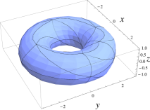
(c) $G^{1}$ octic approximant, $E_{H}$: 0.13

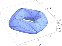
(d) SS approximant, $E_{H}$: 0.45

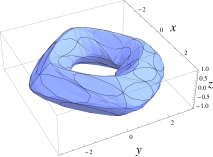
(e) HB approximant, $E_{H}$: 0.59

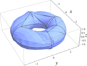
(f) TK approximant, $E_{H}$: 0.26

Figure 9: Approximation of the torus by different interpolation schemes. Hausdorff errors ($E_{H}$) are shown next to the plots.

6.2 Free-form surface approximation

In the next example, we approximate an open free-form surface defined by a vector function $\boldsymbol{f}$,

$$\boldsymbol{f}:[-3,\,3]^{2}\to\mathbb{R}^{3},\quad \boldsymbol{f}(u,\,v):=\left(u+\frac{v^{2}}{12},\,v-\cos(u),\,\frac{1}{3}u^{2}+\sin(v)\right).$$

Again, we approximate the surface by different interpolation schemes. Plots are shown in Fig. 10. As in the first test, our two schemes give smaller Hausdorff distance error than SS and HB methods. The referential surface gives a very accurate estimate of the final shape of our two interpolants. To construct an open surface HB approximant, the spline is constructed on a bigger domain and only relevant patches of the surface are presented.

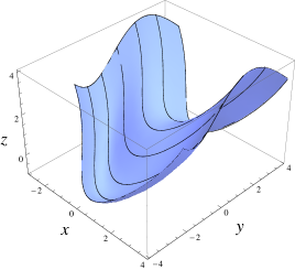
(a) Surface defined by $\boldsymbol{f}$

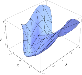
(b) Referential surface

(c) $C^{1}$ quintic scheme, $E_{H}$: 0.051

(d) $G^{1}$ octic scheme, $E_{H}$: 0.050

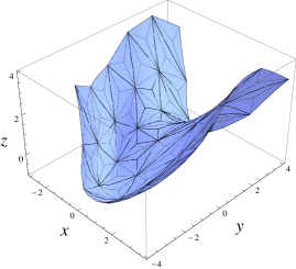
(e) SS scheme, $E_{H}$: 0.14

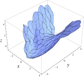
(f) HB scheme, $E_{H}$: 0.36

Figure 10: Approximation of parametric function $\boldsymbol{f}$ by different interpolation schemes. Hausdorff errors ($E_{H}$) are shown next to the plots.

6.3 Approximation of a scalar function

In the following example our scheme is compared against functional Argyris interpolant. We approximate a function $f$,

$$f:[-2,\,2]^{2}\to\mathbb{R},\quad f(u,\,v):=1/2\,\sin(u\,v).$$

The resulting interpolants are visually almost indistinguishable (Fig. 11). Better accuracy of the Argyris element is expected since it interpolates a much larger set of scalar data that are related to the parameterization, whereas the $C^{1}$ quintic element interpolates only geometric data.

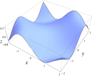
(a) Surface defined by $f$

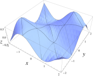
(b) $C^{1}$ quintic approximant, $E_{\max}:~{}0.060$

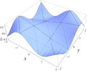
(c) Argyris approximant, $E_{\max}:~{}0.015$

Figure 11: Approximation of function f by the parametric $C^{1}$ quintic scheme and the functional Argyris interpolant. Maximal z-errors ($E_{\max}$) are shown next to the plots.

6.4 Numerical test of the approximation order

Since not all of the control points in our scheme are used for approximation, we cannot expect the optimal convergence rate in the general case. The scheme reproduces linear functions, hence the approximation order is at least 2. On each patch 27 scalar data are used for approximation, a number which is close to 30 scalar degrees of freedom of a cubic parametric patch. Therefore, we can speculate that our scheme will approximate well cubic patches and the order of approximation should be 4 in the majority of cases. This observation is confirmed with two numerical tests. In the first one we approximate a unit sphere and in the second function $f=1/2\,\sin(u\,v)$ from the previous example. For the unit sphere case we compare the radial distance error and in the latter case the Hausdorff distance error against the size of triangles in a triangulation. Convergence plots are depicted in Fig. 12.

(a) Convergence: sphere approximation

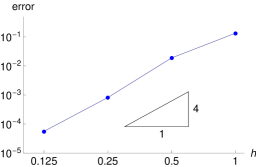
(b) Convergence: approximation of function $f$

Figure 12: Convergence plots: error versus the size of triangles ($h$) in triangulation.

7 Conclusions

In the paper we present a novel Hermite parametric interpolation scheme on triangulations. To construct the interpolant, small local systems of equations need to be solved. Two variants of the scheme are derived: $C^{1}$ quintic and $G^{1}$ octic. The first has fewer degrees of freedom but needs an explicitly given underlying domain triangulation. The second is of higher polynomial degree but can approximate surfaces of arbitrary topology. The scheme focuses on the geometrical construction of good boundary curves - an important feature to obtain a good approximation surface. $C^{2}$ smoothness conditions are imposed at the triangle vertices to overcome the twist compatibility problem.

Numerical examples show that our schemes produce approximants with small distance errors and visually satisfying shapes, even when a small number of patches is used. On a denser grid of interpolation data, the parametric patches visually resemble the functional patches of Argyris elements.

Shape parameters of the interpolant are defined from a referential surface that is based on one step of the Butterfly subdivision scheme. The referential surface gives a basic outline of control points in the space. In the future, the shape parameters could be additionally optimized by applying some energy minimization technique. In that case, control points obtained from the referential surface can be treated as a good starting set of parameters for the optimization procedure. Proper exploitation of the additional six interior control points in $G^{1}$ octic patches remains an open problem for future work. Combining both scheme variations would results in an adaptive and robust scheme with small number of degrees of freedom. For example, $G^{1}$ continuity could be applied only around extraordinary vertices. Another interesting but challenging problem would be to modify parts of the scheme to get the optimal (or near optimal) convergence order while maintaining robustness and desired geometric properties of the scheme.

References

• [1] P. Alfeld, L. L. Schumaker, Smooth macro-elements based on Powell-Sabin triangle splits, Adv. Comp. Math. 16 (1) (2002) 29–46. doi:10.1023/A:1014299228104.
• [2] V. Baramidze, Minimal energy spherical splines on Clough-Tocher triangulations for Hermite interpolation, Appl. Numer. Math. 62 (9) (2012) 1077–1088.
• [3] A. Bobenko, P. Schröder, Discrete willmore flow, in: M. Desbrun, H. Pottmann (Eds.), Eurographics Symposium on Geometry Processing, Eurographics Association, Vienna, 2005, pp. 101–110.
• [4] P. G. Ciarlet, The Finite Element Method for Elliptic Problems, North-Holland, Amsterdam, 1978.
• [5] R. W. Clough, J. L. Tocher, Finite element stiffness matrices for analysis of plates in bending, in: Proceedings of the Conference on Matrix Methods in Structural Mechanics, Wright Patterson A.F.B, Ohio, 1965, pp. 515–545.
• [6] N. Dyn, D. Levin, J. Gregory, A butterfly subdivision scheme for surface interpolation with tension control, ACM Trans. Graph. 9 (2) (1990) 160–169.
• [7] G. Farin, Smooth interpolation to scattered $3$D data, in: R. Barnhill, W. Boehm (Eds.), Surfaces in computer aided geometric design (Oberwolfach, 1982), North-Holland, Amsterdam, 1983, pp. 43–63.
• [8] G. Farin, Curves and surfaces for computer-aided geometric design, 5th Edition, Computer Graphics and Geometric Modeling, Academic Press Inc., San Diego, CA, 2002.
• [9] G. E. Fasshauer, L. L. Schumaker, Minimal energy surfaces using parametric splines, Comput. Aided Geom. Design 13 (1) (1996) 45–79. doi:10.1016/0167-8396(95)00006-2.
• [10] S. Hahmann, G.-P. Bonneau, Triangular ${G}^{1}$ interpolation by 4-splitting domain triangles, Comput. Aided Geom. Design 17 (8) (2000) 731–757.
• [11] G. Herron, Smooth closed surfaces with discrete triangular interpolants, Comput. Aided Geom. Design 2 (4) (1985) 297–306.
• [12] G. Jaklič, On the dimension of the bivariate spline space $S_{3}^{1}(\Delta)$, Int. J. Comput. Math. 82 (11) (2005) 1355–1369.
• [13] G. Jaklič, T. Kanduč, Hermite interpolation by triangular cubic patches with small Willmore energy, Int. J. Comput. Math. 90 (9) (2013) 1881–1898.
• [14] G. Jaklič, T. Kanduč, On positivity of principal minors of bivariate Bézier collocation matrix, Appl. Math. Comput. 227 (2014) 320–328.
• [15] G. Jaklič, J. Kozak, M. Krajnc, V. Vitrih, E. Žagar, On geometric Lagrange interpolation by quadratic parametric patches, Comput. Aided Geom. Design 25 (6) (2008) 373–384.
• [16] M.-J. Lai, L. L. Schumaker, Macro-elements and stable local bases for splines on Clough-Tocher triangulations, Numer. Math. 88 (1) (2001) 105–119. doi:10.1007/PL00005435.
URL http://dx.doi.org/10.1007/PL00005435
• [17] M.-J. Lai, L. L. Schumaker, Spline functions on triangulations, Vol. 110 of Encyclopedia of Mathematics and its Applications, Cambridge University Press, Cambridge, 2007. doi:10.1017/CBO9780511721588.
URL http://dx.doi.org/10.1017/CBO9780511721588
• [18] S. Mann, M. Lounsbery, C. Loop, D. Meyers, J. Painter, T. DeRose, K. Sloan, A survey of parametric scattered data fitting using triangular interpolants, in: G. E. Farin, R. E. Barnhill, H. Hagen (Eds.), Curve and Surface Design, SIAM, 1992, pp. 145–172.
• [19] J. Morgan, R. Scott, A nodal basis for ${C}^{1}$ piecewise polynomials of degree $n\geq 5$, Math. Comp. 29 (131) (1975) 736–740.
• [20] L. Ramshaw, Blossoms are polar forms, Comput. Aided Geom. Design 6 (4) (1989) 323–358.
• [21] L. Shirman, C. Séquin, Local surface interpolation with Bézier patches, Comput. Aided Geom. Design 4 (4) (1987) 279–295.
• [22] L. Shirman, C. Séquin, Local surface interpolation with Bézier patches: errata and improvements, Comput. Aided Geom. Design 8 (3) (1991) 217–221.
• [23] W.-H. Tong, T.-W. Kim, High-order approximation of implicit surfaces by ${G}^{1}$ triangular spline surfaces, Comput. Aided Design 41 (6) (2009) 441–455.
• [24] D. J. Walton, D. S. Meek, A triangular ${G}^{1}$ patch from boundary curves, Comput. Aided Design 28 (2) (1996) 113–123.
• [25] T. Zhou, D. Han, M.-J. Lai, Energy minimization method for scattered data Hermite interpolation, Appl. Numer. Math. 58 (5) (2008) 646–659. doi:10.1016/j.apnum.2007.02.006.
URL http://dx.doi.org/10.1016/j.apnum.2007.02.006
• [26] M. Zlámal, On the finite element method, Numer. Math. 12 (5) (1968) 394–409.
• [27] D. Zorin, P. Schröder, W. Sweldens, Interpolating subdivision for meshes with arbitrary topology, in: Computer Graphics Proceedings (SIGGRAPH 96), ACM, New York, 1996, pp. 189–192.