Generalised Dining Philosophers as Feedback Control

Abstract

We revisit the Generalised Dining Philosophers problem through the perspective of feedback control. The result is a modular development of the solution using the notions of system and system composition (the latter due to Tabuada) in a formal setting that employs simple equational reasoning. The modular approach separates the solution architecture from the algorithmic minutiae and has the benefit of simplifying the design and correctness proofs.

Three variants of the problem are considered: N=1, and N > 1 with centralised and distributed topology. The base case (N=1) reveals important insights into the problem specification and the architecture of the solution. In each case, solving the Generalised Dining Philosophers reduces to designing an appropriate feedback controller.

1 Introduction: The Dining Philosophers problem

Resource sharing amongst concurrent, distributed processes is at the heart of many computer science problems, specially in operating, distributed embedded systems and networks. Correct sharing of resources amongst processes must not only ensure that a single, non-sharable resource is guaranteed to be available to only one process at a time (safety), but also starvation-freedom – a process waiting for a resource should not have to wait forever. Other complexity metrics of interest in a solution are average or worst case waiting time, throughput, etc. Distributed settings introduce other concerns: synchronization, faults, etc.

The Dining Philosophers problem, originally formulated by Edsger Dijkstra in 1965 and subsequently published in 1971[9] is a celebrated thought experiment in concurrency control: Five philosophers are seated around a table. Adjacent philosophers share a fork. A philosopher may either eat or think, but can also get hungry in which case he/she needs the two forks on either side to eat. Clearly, this means adjacent philosophers do not eat simultaneously, the exclusion condition. Each philosopher denotes a process running continuously and forever that is either waiting (hungry) for a resource (like a file to write to), or using that resource (eating), or having relinquished the resource (thinking). The problem consists of designing a protocol by which no philosopher remains hungry indefinitely, the starvation-freeness condition, assuming each eating session lasts only for a finite time. In addition, the progress condition means that there should be no deadlock: at any given time, at least one philosopher that is hungry should move to eating after a bounded period of time. Note that starvation-freedom implies progress.

The generalisation of the Dining Philosophers involves N philosophers with an arbitrary, non-reflexive neighbourhood. Neighbours can not be eating simultaneously. The generalised problem was suggested and solved by Dijsktra himself[10]. The Generalised Dining Philosophers problem is discussed at length in Chandy and Misra’s book[6]. The Dining Philosophers problem and its generalisation have spawned several variants and numerous solutions throughout its long history and is now staple material in many operating system textbooks.

Individual Philosopher dynamics: Consider a single philosopher who may be in one of three states: thinking, hungry and eating. At each step, the philosopher may choose to either continue to be in that state, or switch to the next state (from thinking to hungry, from hungry to eating, or from eating to thinking again). The dynamics of the single philosopher is shown in Fig. 1. Note that the philosophers run forever.

Figure 1: Philosopher states and transitions

We now consider the Generalised Dining Philosophers problem.

Definition 1.1 (Generalised Dining Philosophers problem).

N philosophers are arranged in a connected conflict graph $G=\mbox{$\langle V,E\rangle$}$ where $V$ is a set of $N=|V|$ philosophers and $E$ is an irreflexive adjacency relation between them.

If each of the N philosophers was to continue to evolve according to the dynamics in Fig. 1, two philosophers sharing an edge in $E$ could be eating together, violating safety. The Generalised Dining Philosophers problem is the following:

Problem: Assuming that no philosopher eats forever in a single stretch, construct a protocol that ensures

1. Safety: No two adjacent philosophers eat at the same time.

2. Starvation-freedom: A philosopher that is hungry eventually gets to eat.

3. Non-intrusiveness: A philosopher that is thinking or eating continues to behave according to the dynamics of Fig. 1.

A “protocol” is usually interpreted as an algorithm or a computer program that runs as part of the process. The protocol defines the interaction between the actors mentioned (philosophers in the generalised problem, and in the 5-diners problem, the forks as well) in the problem that may be needed to solve the problem.

The main actors in this problem are the philosophers. The dynamics of the philosophers’ transitions as shown in Fig. 1 are governed by their choice to either remain in the same state or move to a new state. This choice manifests as non-determinism in the dynamics. The first observation is that the philosopher dynamics as shown in Fig. 1 is inadequate to ensure safety. As noted above, nothing prevents two adjacent and hungry philosophers to both move to eating.

One way of solving the Generalised Dining Philosophers problem is to define a more complex dynamics that each of the N philosophers implements so that the safety and starvation freedom conditions hold. Yet another way, that hints at the control approach, is to consider additional actors that restrain the philosophers’ original actions in some specific and well-defined way so as to achieve safety and starvation freedom. The additional actors needed to restrict the philosophers’ actions are called controllers. The role of the controller is to issue commands that may involve overriding the philosopher’s own choice to move to a new state. For example, a hungry philosopher who wishes to eat in the next cycle may find his/her wish overridden by a command issued by the controller to continue to remain hungry in the interest of preserving the safety invariant. However, in any solution to the problem, the controller should eventually promote a hungry philosopher to eating so as to preserve the starvation freedom invariant. It is this approach that we wish to explore in this paper.

Any control on the philosophers should be not overly restrictive: a philosopher who is either thinking or eating should be allowed to exercise his/her choice about what to do next; only a hungry philosopher may be commanded by the controller either to continue to remain hungry or switch to eating, overriding the philosopher’s own choice of whether to stay hungry or switch to eating.

Solutions to the Generalised Dining Philosophers may be broadly classified as either centralised or distributed. The centralised approach assumes a central controller that commands the philosophers on what to do next. The distributed approach assumes no such centralised authority; the philosophers are allowed to communicate to arrive at a consensus on what each can do next.

The objective of this paper is to formulate the Generalised Dining Philosophers problem using the idea of control, particularly that which involves feedback. Feedback control, also called supervisory control, is the foundation of much of engineering science and is routinely employed in the design of embedded systems. However, its value as a software architectural design principle is only insufficiently captured by the popular “model-view-controller” (MVC) design pattern[13], usually found in the design of user and web interfaces. For example, MVC controllers implement open loop instead of feedback control.

The starting point is a more precise statement of the problem by employing the formalism of discrete state transition systems with output, also called Moore machines. We then borrow the notion of system composition due to Tabuada[33]. Composition is defined with respect to an interconnect that relates the states and inputs of the two systems being composed. Viewed from this perspective, the Generalised Dining Philosophers form a system consisting of interconnected subsystems. A special case of the interconnect which relates inputs and outputs yields modular composition and allows the Generalised Dining Philosophers to be treated as an instance of feedback control. The solution then reduces to designing two types of components - the philosophers and the controllers - and their interconnections (the system architecture), followed by definitions of the transition functions of the philosophers and the controllers. The transition function of the controller is called a control law.

The compositional approach encourages us to think of the system in a modular way, emphasising the interfaces between components and their interconnections. One benefit of this approach is that it allows us to define multiple types of controllers (N=1, N>1 centralised and N>1 local) that interface with a fixed philosopher system. The modularity in architecture also leads to modular correctness proofs of safety and starvation freedom. For example, the proof of the distributed case is reduced to showing that the centralised controller state is reconstructed by the union of the states of the distributed local controllers. That said, however, subtle issues arise even in the simplest variants of the problem. These have to do with non-determinism, timing and feedback, but equally, from trying to seek a precise definition of the problem itself.

Paper roadmap

The rest of the paper is an account on how to solve the Generalised Dining Philosophers problem in a step-by-step manner, varying both the complexity of the problem from N=1 to N>1 and from centralised to distributed. We begin with a short review of the fundamental concept of systems, their behaviour and composition (Section 2) and the role of time. We then turn our attention to the simplest variant of the Generalised Dining Philosophers: the 1 Diner problem (Section 3) and explore a series of architectures for the single philosopher, the controller and their composition. The architecture identifies the boundaries and interfaces of each subsystem and the “wiring” of the subsystems, in this case, the one philosopher and the controller, with each other. Next we consider N Diners (Section 4), where the problem reduces to designing a controller and (a) defining a data structure internal to the controller’s state and an algorithm to manipulate it and, (b) computing the set of control inputs. After proving the correctness of the centralised solution, we consider distributed control (Section 5). The problem here reduces to distributing the effort of the centralised controller to N different local controllers, each controlling the behaviour of its corresponding philosopher. A clear interconnect boundary between each component defines exactly which part of the state is shared between the components. We compare the feedback control based solution with other approaches (Section 6) and conclude with some pointers to future work (Section 7).

No prior background in control theory is assumed; relevant concepts from control systems are explained in the next section.

2 Systems Approach

The main idea in control theory is that of a system. Systems have state and exhibit behaviour governed by a dynamics. A system’s state undergoes change due to input. Dynamics is the unfolding of state over time, governed by laws that relate input with the state. A system’s dynamics is thus expressed as a relation between the current state, the current input and the next state. Its output is a function of the state. Thus inputs and outputs are connected via state. The system’s state is usually considered hidden, and is inaccessible directly. The observable behaviour of a system is available only via its output. A schematic diagram of a system is shown in Figure 2.

Figure 2: System with input and output

In control systems, we are given a system, often identified as the plant. The plant is also referred to as model in the literature and we shall use the two terms interchangeably. The plant exhibits a certain observable behaviour. The behaviour may be informally described as an infinite sequence of input-output pairs. In addition to the plant, we are also given a target behaviour that is usually a restriction of the plant’s behaviour.

There are many ways of realising the target behaviour. The first is to attach another system, an output filter, that takes the output of the plant and suitably modifies it, so that the resulting output now conforms to the behaviour specified in the problem. A second way is to have a system, input filter, that intercepts the inputs to the plant, suitably modifies (or restricts) them and then feeds the results to the plant. In both cases, the architecture of the plant is left untouched. The dynamics of the plant too remains unaffected. Restricting the input is, however, not always possible.

There is a third way to influence the plant to achieve the specified behaviour, which is usually what is referred to as control. The control problem is, very roughly, the following: what additional input(s) should be supplied to the plant, such that the resulting dynamics as determined by a new relation between states and inputs now exhibits output behaviour that is either equal or approximately equal to the target behaviour specified in the problem? The additional input is usually called the forced or control input. Notice that the additional inputs may require altering the interface and the dynamics of the plant. The plant’s altered dynamics need to take into account the combined effect of the original input and the control input.

The second design question is how should the control input be computed. Often the control input is computed as a function of the output of the plant (now extended with the control input). Thus we have another system, the controller, (one of) whose inputs is the output of the plant and whose output is (one of) the inputs to the plant. This architecture is called feedback control. The relation between the controller’s input and its state and output is called a control law.

Figure 3 is a schematic diagram representing a system with feedback control.

Figure 3: Feedback Control System

The principle of feedback control is well studied and is used extensively in building large-scale engineering systems of wide variety. A modern introduction to the subject is the textbook by Åström and Murray[2] which motivates the subject by illustrating the use of feedback control in various engineering and scientific domains: electrical, mechanical, chemical, and biological and also computing.

In the rest of this section, we present the formal notion of a system and system composition as defined by Tabuada[33].

2.1 Specification, instance and behaviour

A system specification (or type) is a tuple with six fields:

$$S=\mbox{$\langle x:X,x^{0}:X^{0},u:U,\stackrel{{\scriptstyle[}}{{S}}]{}{\longrightarrow},y:Y,h\rangle$}$$

$X$, a set of states is called the state space of the system $S$. $X^{0}\subseteq X$ is the set of initial states. $U$ is the input space. $\stackrel{{\scriptstyle[}}{{]}}{}{\longrightarrow}\subseteq X\times\ U\times X$ is the input-state transition relation describing the set of possible transitions, that is the dynamics. $Y$ is the output space, and $h:X\longrightarrow Y$ is the output function that maps states to outputs. We elide the component $X^{0}$ if $X^{0}=X$. $U$ is unitary if it is a singleton $\{*\}$. We elide $U$, $Y$ or $h$ if $U$ is unitary, $Y=X$ or $h$ is identity, respectively.

Notation 2.1.

$S$ is to be seen as a record with canonical field names $X$, $U$, $X^{0}$, $\stackrel{{\scriptstyle[}}{{S}}]{}{\longrightarrow}$, $Y$ and $h$. These names are associated with values when a system is defined. When a system is defined, we indicate the values in place, say if $X$ equals $A$, we write $S=\mbox{$\langle X=A,\ldots\rangle$}$. The lowercase names $x$,$x^{0}$,$u$ and $y$ denote system variables that range over $X$, $X^{0}$, $U$ and $Y$ respectively. Their values define the configuration of the system at any point in its evolution: the value of the state, the initial state, input, and output. A field or system variable like $X$ or $x$ of a system $S$ is written $X_{S}$, alternatively $S.X$. When $S$ is clear from the context, the subscript is omitted. Often, additional variable names (aliases) are used. E.g., in the philosopher system $Q$ defined later, the name $x$ denoting the state system variable is aliased to $a$. We write $S=\mbox{$\langle a:X=A,\ldots,\rangle$}$ to denote that the state space field $X$ has the value $A$, and the variable name $a$ is an alias to the (default) state variable $x$.

$S$ is deterministic if the relation $\stackrel{{\scriptstyle[}}{{S}}]{}{\longrightarrow}$ is a partial function, non-deterministic otherwise. The transition relation in a deterministic system is usually denoted by a transition function $f:X\times U\rightarrow X$. A system is autonomous if $U_{S}$ is unitary, non-autonomous otherwise. A system is transparent, or white box if its output function $h$ is identity.

A system instance $s$ of type $S$, denoted $s:S$, is a record consisting of three fields $\langle x:X_{S},u:U_{S},y:Y_{S}\rangle$. The fields of $s$ are accessed via the dot notation. E.g., $s.x$, etc. We also write $s.X$ to mean $S.X$ where $s:S$, etc. Often times, we overload a system specification $S$ to also denote its instance. Thus $x_{S}$ denotes the state of the system instance of type $S$, etc.

2.2 System composition

A complex system is best described as a composition of interconnected subsystems. We employ the key idea of an interconnect due to Tabuada[33]. An interconnect between two systems is a relation that relates the states and the inputs of two systems.

Let $S_{c}=\mbox{$\langle X_{c},X_{c}^{0},U_{c},\stackrel{{\scriptstyle[}}{{c}}]{}{\longrightarrow},Y_{c},h_{c}\rangle$}$ and $S_{a}=\mbox{$\langle X_{a},X_{a}^{0},U_{a},\stackrel{{\scriptstyle[}}{{a}}]{}{\longrightarrow},Y_{a},h_{a}\rangle$}$ be two systems, then ${\cal{I}}\subseteq X_{c}\times X_{a}\times U_{c}\times U_{a}$ is called an interconnect relation. Informally, an interconnect specifies the architecture of the composite system.

The composition $S_{c}\times_{{\cal{I}}}S_{a}$ of $S_{c}$ and $S_{a}$ with respect to the interconnect ${\cal{I}}$ is defined as the system $S_{ca}=\mbox{$\langle X_{ca},X_{ca}^{0},U_{ca},\stackrel{{\scriptstyle[}}{{c}}a]{}{\longrightarrow},Y_{ca},h_{ca}\rangle$}$, where

1. $X_{ca}=\mbox{$\{(x_{c},x_{a})\ |\ \exists u_{c},u_{a}.(x_{c},x_{a},u_{c},u_{a})\in{\cal{I}}\}$}$

2. $X^{0}_{ca}=X_{ca}\cap(X^{0}_{c}\times X^{0}_{a})$

3. $U_{ca}=U_{c}\times U_{a}$

4. $(x_{c},x_{a})\stackrel{{\scriptstyle[}}{{c}}a]{u_{c},u_{a}}{\longrightarrow}(x^{\prime}_{c},x^{\prime}_{a})$ iff

   1. $x_{c}\stackrel{{\scriptstyle[}}{{c}}]{u_{c}}{\longrightarrow}x^{\prime}_{c}$,

   2. $x_{a}\stackrel{{\scriptstyle[}}{{a}}]{u_{a}}{\longrightarrow}x^{\prime}_{a}$, and

   3. $(x_{c},x_{a},u_{c},u_{a})\in{\cal{I}}$

5. $Y_{ca}=Y_{c}\times Y_{a}$

6. $h_{ca}(x_{c},x_{a})=(h_{c}(x_{c}),h_{a}(x_{a}))$.

Notation 2.2 (Components of a composite).

If $D=C\times_{{\cal{I}}}A$ then $D.C$ and $D.A$ refer to the projections of the respective subsystems. The individual values e.g., $D.C.x$ and $D.A.x$ are abbreviated $D.x_{C}$ and $D.x_{A}$. When the composition $D$ is clear from the context, we continue to use $x_{C}$ and $x_{A}$, etc.

The restrictions of systems $A$ and $C$ are embedded as subsystems in the composite system. The interconnected system $A$ is different from the $A$ that is unconnected. The former’s dynamics is governed by the additional constraints imposed by the interconnect. Often we will define a system $A$, and then its composition with another system. Subsequent references to $A$ and its behaviour refer to the interconnected (and hence constrained) subsystem of the composite system. This could occasionally lead to some ambiguity, specially when the interconnect is not clear from the context. In such a case, the context will be made clear.

Second, since the interconnect completely defines the composite system, we will limit our description of the composite system to the individual subsystems and the interconnect relation and rarely write down the components of the composite systems.

The notion of Tabuada composition subsumes several other notions of composition.

Example 2.1 (Synchronous Composition).

The synchronous composition [16, 25], also called “parallel composition with shared actions” [24], is one in which two systems have input alphabets with possibly non-empty intersection. The two systems simultaneously transition on any input that is in the intersection; otherwise, each system transition to the input that is in its input space, the other process does not advance.

The synchronous composition $S_{c}\times_{H}S_{a}$ of two white box systems $S_{c}$ and $S_{a}$ is given by

$$S_{c}\times_{H}S_{a}=\mbox{$\langle X_{c}\times X_{a},X^{0}_{c}\times X^{0}_{a},U_{c}\cup U_{a},\stackrel{{\scriptstyle[}}{{H}}]{}{\longrightarrow}\rangle$}$$

where

1. $(x_{c},x_{a})\stackrel{{\scriptstyle[}}{{H}}]{u}{\longrightarrow}(x^{\prime}_{c},x^{\prime}_{a})$ if $u\in U_{c}\cap U_{a}$, $x_{c}\stackrel{{\scriptstyle[}}{{c}}]{u}{\longrightarrow}x^{\prime}_{c}$ and $x_{a}\stackrel{{\scriptstyle[}}{{a}}]{u}{\longrightarrow}x^{\prime}_{a}$

2. $(x_{c},x_{a})\stackrel{{\scriptstyle[}}{{H}}]{u}{\longrightarrow}(x^{\prime}_{c},x_{a})$ if $u\in U_{c}\setminus U_{a}$, $x_{c}\stackrel{{\scriptstyle[}}{{c}}]{u}{\longrightarrow}x^{\prime}_{c}$

3. $(x_{c},x_{a})\stackrel{{\scriptstyle[}}{{H}}]{u}{\longrightarrow}(x_{c},x^{\prime}_{a})$ if $u\in U_{a}\setminus U_{c}$, $x_{a}\stackrel{{\scriptstyle[}}{{a}}]{u}{\longrightarrow}x^{\prime}_{a}$

This may be expressed as a Tabuada composition over systems whose input spaces are lifted by a fresh element $\bot$, distinct from elements in $U_{c}\cup U_{a}$.

$$S_{c^{\prime}}=\mbox{$\langle X_{c},X^{0}_{c},U_{c}\cup\mbox{$\{\bot\}$},\stackrel{{\scriptstyle[}}{{c}}^{\prime}]{}{\longrightarrow}\rangle$}$$

$$S_{a^{\prime}}=\mbox{$\langle X_{a},X^{0}_{a},U_{a}\cup\mbox{$\{\bot\}$},\stackrel{{\scriptstyle[}}{{a}}^{\prime}]{}{\longrightarrow}\rangle$}$$

where

1. $\stackrel{{\scriptstyle[}}{{c}}^{\prime}]{}{\longrightarrow}=\stackrel{{\scriptstyle[}}{{c}}]{}{\longrightarrow}\cup\mbox{$\{x\stackrel{{\scriptstyle[}}{{c}}^{\prime}]{\bot}{\longrightarrow}x\ |x\in X_{c}\}$}$

2. $\stackrel{{\scriptstyle[}}{{a}}^{\prime}]{}{\longrightarrow}=\stackrel{{\scriptstyle[}}{{a}}]{}{\longrightarrow}\cup\mbox{$\{x\stackrel{{\scriptstyle[}}{{a}}^{\prime}]{\bot}{\longrightarrow}x\ |x\in X_{a}\}$}$

The interconnect ${\cal{I}}_{H}$ is defined as ${\cal{I}}_{H}\subseteq X_{c}\times X_{a}\times(U_{c}\cup{\bot})\times(U_{a}\cup{\bot})$, where

$$(x_{c},x_{a},u_{c},u_{a})\in{\cal{I}}_{H}\ \mbox{iff}$$

any of the following hold:

$$u_{a}=u_{c} \quad\mbox{and}\quad u_{a}\in U_{a}\cap U_{c},\ \mbox{or}$$

$$u_{a}=\bot \quad\mbox{and}\quad u_{c}\in U_{c}\setminus U_{a},\ \mbox{or}$$

$$u_{c}=\bot \quad\mbox{and}\quad u_{a}\in U_{a}\setminus U_{c}$$

It is a simple exercise to verify that $(x_{c},x_{a})\stackrel{{\scriptstyle[}}{{H}}]{u}{\longrightarrow}(x^{\prime}_{c},x^{\prime}_{a})$ iff $(x_{c},x_{a})\stackrel{{\scriptstyle[}}{{{\cal{I}}}}_{H}]{(u_{c},u_{a})}{\longrightarrow}(x^{\prime}_{c},x^{\prime}_{a})$.

2.3 Modular interconnects

While interconnects can, in general, relate states, the interconnects designed in this paper are modular: they relate inputs and outputs. Defining a modular interconnect is akin to specifying a wiring diagram between two systems. Modular interconnects drive modular design.

2.4 Time

The Generalised Dining Philosophers problem refers to time in the assumption (“forever”) and the safety (at the “same time”) and starvation freedom requirements (“eventually”). Therefore, any solution to the Generalised Dining Philosophers problem will need to be based on a model of time that addresses both simultaneity and eternity.

It is useful to interpret $x\stackrel{{\scriptstyle[}}{{]}}{u}{\longrightarrow}x^{\prime}$ happening over time: the system is first in state $x$, and then as a result of input $u$, it comes into the state $x^{\prime}$. Nothing, however is mentioned about when that transition happens in the formal definition of a system. It is therefore, necessary to introduce an explicit notion of time as part of the system’s dynamics. There are several models of time, but the modelling of time in systems is subtle[20, 21]. Models range from ordinal time which denotes the number of transitions made by the system, to physical time as a non-negative positive real number. We assume that the reference to time in the Generalised Dining Philosophers problem is to physical time and not ordinal time because the Philosophers represent processes executing in physical time. Given this assumption, the Generalised Dining Philosophers is a good example of the inadequacy of ordinal time. Consider two adjacent philosophers $A$ and $B$ and their trajectories in real time (Table 1). Each philosopher, after the second step is in the eating state. But these steps are disjoint in physical time: $A$ is eating from 2.0 to 7.0 seconds, whereas $B$ doesn’t start eating till 8.0 seconds. Although $A[2]={\sf{e}}=B[2]$, these states do not coincide in physical time. The converse may also happen: $A$ and $B$’s states do not coincide in ordinal time, but coincide in physical time ($t=12.0s$ onward in Table 1). See Fig. 4.

Table 1: Trajectories of states of two philosophers over physical time. Note that ordinal time $i$ of the two philosophers need not correspond to the same continuous time. This table illustrates why it is necessary to account for continuous (real) time rather than logical time for the Generalised Dining Philosophers problem.

Time (sec)	Event	$A$’s state	$B$’s state
0		$A[0]={\sf{t}}$	$B[0]={\sf{t}}$
1.0	$A1:{\sf{t}}\stackrel{{\scriptstyle[}}{{]}}{}{\longrightarrow}{\sf{h}}$	$A[1]={\sf{h}}$
2.0	$A2:{\sf{h}}\stackrel{{\scriptstyle[}}{{]}}{}{\longrightarrow}{\sf{e}}$	$A[2]={\sf{e}}$
5.0	$B1:{\sf{t}}\stackrel{{\scriptstyle[}}{{]}}{}{\longrightarrow}{\sf{h}}$		$B[1]={\sf{h}}$
7.0	$A3:{\sf{e}}\stackrel{{\scriptstyle[}}{{]}}{}{\longrightarrow}{\sf{t}}$	$A[3]={\sf{t}}$
8.0	$B2:{\sf{h}}\stackrel{{\scriptstyle[}}{{]}}{}{\longrightarrow}{\sf{e}}$		$B[2]={\sf{e}}$
11.0	$A4:{\sf{t}}\stackrel{{\scriptstyle[}}{{]}}{}{\longrightarrow}{\sf{h}}$	$A[4]={\sf{h}}$
12.0	$A5:{\sf{t}}\stackrel{{\scriptstyle[}}{{]}}{}{\longrightarrow}{\sf{e}}$	$A[5]={\sf{e}}$

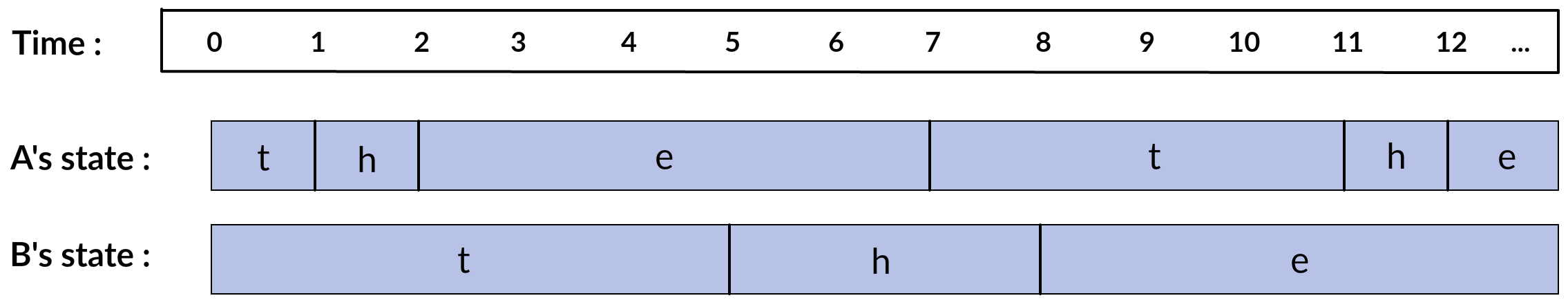
Figure 4: Trajectories of two processes $A$ and $B$ over ordinal and physical time.

We employ the idea from time triggered architecture [19] which is based on a global clock with fixed time period against which all subsystems transitions are synchronised, much like in a hardware circuit. The global clock ticks with a fixed time period $\tau>0$. All systems share the global clock and transitions are synchronised to occur in step with the clock. Values exist over continuous time, but are polled at regular fixed intervals. If $t\in\mathbb{N_{0}}$, $x[t]$ means the value of $x$ at physical time $t\tau$. Furthermore, the transitions of all subsystems are synchronised: the $t$th transition of each subsystem is transacted at exactly the same physical time for each subsystem. Transitions are assumed to not be instantaneous. If input is available at clock cycle $t$, then the output of the new state as a result of the transition is available only one clock cycle later.

With clocked time, the composite system’s dynamics may be described as evolving over the same clock time as that of the subsystems’ dynamics. Furthermore, since transitions are not instantaneous but incur a delay, feedback becomes easier to model. Such a model has already been successfully adopted by the family of synchronous reactive languages like Esterel, Lustre and Signal[12, Chap 2]. Furthermore, extracting asynchronous behaviour becomes a matter of making assumptions on the relative time periods between input events and the computation of outputs.

2.5 Clocked Systems

The notion of a system is general enough to be able to model a clock and also a system whose transitions are synchronised with the ticks of the clock.

Notation 2.3.

Let

$$B=\mbox{$\{0,1\}$}$$

denote a set of binary values and let $b$ range over $B$.

2.5.1 Clock as a system

A clock ticking every $\tau$ units of time may be modelled as a system $K$ whose state is time and whose input is an arbitrary non-negative interval of time. A state $x$ relates to $x^{\prime}$ via time interval $u$ if $x^{\prime}=x+u$. The tick is modelled as an impulse occurring at multiples of $\tau$.

$$K(\tau)=\mbox{$\langle X,X^{0},U,f:X,U\rightarrow X,Y,h\rangle$}$$

where

• $X={\mathbb{R}}^{\geq 0}$

• $X^{0}=\mbox{$\{0\}$}$

• $U={\mathbb{R}}^{>0}$

• $f(x,u)=x+u$

• $Y=B$

• $h(x)=1$ if $x=n\tau$ for some $n\in\mathbb{N_{0}}$, $0$ otherwise.

2.5.2 Extending a system interface to accommodate a clock

To synchronise a system $S$ with a clock, it is first necessary to extend the interface of the system to accommodate an additional input of type $B$. The extension $S^{K}$ of $S$ is $S^{K}=\mbox{$\langle X,X^{0},U,\stackrel{{\scriptstyle[}}{{S}}^{K}]{}{\longrightarrow},Y,h\rangle$}$ where

• $X=X_{S}$

• $X^{0}=X^{0}_{S}$

• $U=U_{S}\times B$

• $x\stackrel{{\scriptstyle[}}{{S}}^{K}]{u_{S},b}{\longrightarrow}x^{\prime}$ iff $x\stackrel{{\scriptstyle[}}{{S}}]{u_{S}}{\longrightarrow}x^{\prime}$ and $b=1$.

• $Y=Y_{S}$

• $h=h_{S}$

$S^{K}$ makes a transition only if it is admissible by the underlying system $S$ and its second input is 1.

2.5.3 Synchronising a system with a clock

The interconnect ${\cal{I}}$ wires the clock’s output as the second input of $S^{K}$:

$${\cal{I}}=\mbox{$\{(x_{K},x_{S},u_{K},u_{S},b)\ |\ h_{K}(x_{K})=b\}$}$$

In the composite system $T=K\times_{{\cal{I}}}S^{K}$, the transitions of a system $S^{K}$ are now synchronised to occur at each clock tick. That is, the component $x_{S^{K}}$ of $x_{T}$ is constant during the semi-open interval $[i\tau,(i+1)\tau)$ and changes only at multiples of $\tau$. Thus we may now treat $x_{S^{K}}$ (and $y_{S^{K}}$) as functions over $\mathbb{N_{0}}$, the set of naturals. Furthermore, inputs occurring at other than instances of the clock ticks effect no change of state.

From here on, we will not explicitly model the clock or its composition with systems. Instead, we assume that all systems we design are implicitly clocked and there is one global clock that drives all the subsystems of a system.

The dynamics of a system $S=\mbox{$\langle X,X^{0},U,\stackrel{{\scriptstyle[}}{{S}}]{}{\longrightarrow},Y,h\rangle$}$ suitably extended and interconnected with a clock may now be described as a discrete dynamical system:

$$x[i]\stackrel{{\scriptstyle[}}{{S}}]{u[i]}{\longrightarrow}x[i+1]$$ (1)

$$y[i]=h(x[i])$$ (2)

where $i\in\mathbb{N_{0}}$ denotes the $i$th clock cycle and $x$, $u$ and $y$ are functions from $\mathbb{N_{0}}$ to $X$, $U$, and $Y$ respectively.

Notation 2.4.

For the sake of convenience, but at the risk of introducing some ambiguity, we use the notation $x$ to mean $x[i]$ and $x^{\prime}$ to mean $x[i+1]$, the value at the next clock cycle. Likewise for other variables.

3 The One Dining Philosopher problem

We start with N=1, the simplest case of the problem. The 1 Diner problem is simple, but not trivial. Indeed, as we shall see, it reveals important insights about both the problem structure and its solution for the general (N>1) case.

We now systematise the formal construction of philosopher system connected to a controller via feedback. We start with a philosopher model $Q$ that is completely unconstrained in its behaviour, then build a deterministic model $P$, identical in behaviour with $Q$, but in which $Q$’s non-determinism is encoded as choice input. $P$’s interface is not quite suitable for participating in feedback control. That requires three more steps: First, extending $P$ to the model $M$ which accommodates an additional control input. Second, defining a controller $C$ that generates control input (Section 3.4). Third, wiring the controller with the system $M$ to build a feedback system $R$ (Section 3.5). Timing analysis reveals that because of delays introduced in the feedback, the control input may not arrive in time for it to be useful (Section 3.6). A new input type where the signal is present or absent and a plant $S$ working with this input (Section 3.7) need to be composed with the controller in such a way that the rate at which choice input arrives is synchronised with the rate at which the controller computes its output to yield the system $T$ (Section 3.8).

3.1 Philosopher as an autonomous non-deterministic system

An unconstrained philosopher (free to switch or stay) may be modelled as an autonomous, non-deterministic, transparent system

$$Q=\mbox{$\langle a:X=\mbox{\it Act},a^{0}:X^{0}=\mbox{$\{\sf{t}\}$},\stackrel{{\scriptstyle[}}{{Q}}]{}{\longrightarrow}\rangle$}$$

where $\stackrel{{\scriptstyle[}}{{Q}}]{*}{\longrightarrow}$ is defined via the edges in Fig. 1:

$${\sf{t}}\stackrel{{\scriptstyle[}}{{Q}}]{*}{\longrightarrow}{\sf{t}},\quad \quad{\sf{t}}\stackrel{{\scriptstyle[}}{{Q}}]{*}{\longrightarrow}{\sf{h}}$$

$${\sf{h}}\stackrel{{\scriptstyle[}}{{Q}}]{*}{\longrightarrow}{\sf{h}},\quad \quad{\sf{h}}\stackrel{{\scriptstyle[}}{{Q}}]{*}{\longrightarrow}{\sf{e}}$$

$${\sf{e}}\stackrel{{\scriptstyle[}}{{Q}}]{*}{\longrightarrow}{\sf{e}},\quad \quad{\sf{e}}\stackrel{{\scriptstyle[}}{{Q}}]{*}{\longrightarrow}{\sf{t}}$$

Notation 3.1.

We use the identifier $a$ to range over Act.

3.2 Choice deterministic philosopher

The non-determinism of $Q$ may be externalised by capturing the choice at a state as binary input $b$ of type $B$ to the system.

The resultant system is deterministic with respect to the choice input. On choice $b=0$ the system stays in the same state; on $b=1$ it switches to the new state. This is shown below in the construction of a non-autonomous, deterministic system

$$P=\mbox{$\langle a:X=\mbox{\it Act},a^{0}:X^{0}=\mbox{$\{{\sf{t}}\}$},b:U=B,f_{P}\rangle$}$$

where $f_{P}:\mbox{\it Act}\times B\rightarrow\ \mbox{\it Act}$ is defined as

$$f_{P}(a,0)=\mbox{\it stay}(a)$$ (3)

$$f_{p}(a,1)=\mbox{\it switch}(a)$$ (4)

and $\mbox{\it stay}:\mbox{\it Act}\rightarrow\mbox{\it Act}$ and $\mbox{\it switch}:\mbox{\it Act}\rightarrow\mbox{\it Act}$ are given by

$$\mbox{\it stay}(a) =a$$

$$\mbox{\it switch}({\sf{t}}) ={\sf{h}}$$

$$\mbox{\it switch}({\sf{h}}) ={\sf{e}}$$

$$\mbox{\it switch}({\sf{e}}) ={\sf{t}}$$

The two systems $P$ and $Q$ are equivalent in behaviour.

Proposition 3.1.

${\cal{B}}^{\omega}(Q)={\cal{B}}^{\omega}(P)$.

Proof.

For both systems, the output space and state space are identical and the output functions are identity functions. Thus state and output traces are identical.

${\cal{B}}^{\omega}(Q)\subseteq{\cal{B}}^{\omega}(P)$: For each state trace $\overline{x}$ in ${\cal{B}}^{\omega}(Q)$, we construct an input-state trace in $P$ and show that the corresponding state trace in $P$ is $\overline{x}$.

For each $i\in\mathbb{N_{0}}$, let $a_{i}$ be the $i$th state in the trace $\overline{a}$. Then there is an input-state transition $a\stackrel{{\scriptstyle[}}{{Q}}]{*}{\longrightarrow}a^{\prime}$. If $a=a^{\prime}$, then we construct the transition $a\stackrel{{\scriptstyle[}}{{P}}]{0}{\longrightarrow}a^{\prime}$ of $P$. If $a\neq a^{\prime}$, then we construct the transition $a\stackrel{{\scriptstyle[}}{{P}}]{1}{\longrightarrow}a^{\prime}$.

${\cal{B}}^{\omega}(P)\subseteq{\cal{B}}^{\omega}(Q)$: For the input-state transition $a\stackrel{{\scriptstyle[}}{{P}}]{u}{\longrightarrow}a^{\prime}$, we construct a transition $a\stackrel{{\scriptstyle[}}{{Q}}]{*}{\longrightarrow}a^{\prime}$ in $Q$.

∎

3.3 Interfacing control

The Philosopher $P$ needs to be extended to admit control input. Control is accomplished through control input or command:

$$\mbox{\it Cmd}=\mbox{$\{{\sf{pass}},{\sf{!0}},{\sf{!1}}\}$}$$

Notation 3.2.

We use the identifier $c:\mbox{\it Cmd}$ to denote a command.

The dynamics of a philosopher subject to a choice input combined with a control input may be described as follows. With command $c$ equal to ${\sf{pass}}$, the philosopher follows the choice input $b$. With the command equal to $!\;b$, the input is ignored, and the command prevails in determining the next state of the philosopher according to the value of $b$: stay if $b=0$, switch if $b=1$.

The philosopher system extended with a control input plays the role of a model and is given by the transparent deterministic system

$$M=\mbox{$\langle a:X=\mbox{\it Act},a^{0}:X^{0}=\mbox{$\{{\sf{t}}\}$},(b,c):(U_{P}\times U_{F})=B\times\mbox{\it Cmd},f_{M}\rangle$}$$

where $U_{P}$ denotes the preference (choice) and $U_{F}$ defines the forced (control) input and $f_{M}:\mbox{\it Act}\times(B\times\mbox{\it Cmd})\rightarrow\mbox{\it Act}$ is given by

$$f_{M}(a,b,{\sf{pass}}) =f_{P}(a,b)$$

$$f_{M}(a,\_,!\;b) =f_{P}(a,b)$$

(In the second case, $\_$ indicates an unnamed formal parameter whose name is not relevant because it is never used subsequently.)

3.4 Controller

A controller is a transparent deterministic system $C$ whose input is an activity and whose output is a control signal of type Cmd. The controller’s role is to examine its input and compute an output command based on the following control law: if its input is ${\sf{h}}$, then the output is ${\sf{!1}}$, otherwise it is ${\sf{pass}}$. The controller’s state space is Cmd with initial state ${\sf{pass}}$ and its input $a$ is an activity.

$$C=\mbox{$\langle c:X=\mbox{\it Cmd},c^{0}:X^{0}=\mbox{$\{{\sf{pass}}\}$},a:U=\mbox{\it Act},f_{C}\rangle$}$$

and $f_{C}:\mbox{\it Cmd}\times\mbox{\it Act}\rightarrow\mbox{\it Cmd}$ is defined as

$$f_{C}(c,a) =g_{C}(a)$$

$$g_{C}({\sf{h}}) ={\sf{!1}}$$

$$g_{C}({\sf{e}}) ={\sf{pass}}$$

$$g_{C}({\sf{t}}) ={\sf{pass}}$$

3.5 Feedback composition

Consider the interconnect ${\cal{I}}_{R}\subseteq X_{C}\times X_{M}\times U_{C}\times U_{M}$, between the controller $C$ and the model $M$

$${\cal{I}}_{R}=\mbox{$\{(C.y,M.y,C.u,(M.b,M.c))|M.y=C.u,C.y=M.c\}$}$$

${\cal{I}}_{R}$ specifies feedback composition since it connects the philosopher’s output $M.a$ to the input of the controller $C.a$ and the controller’s output $C.c$ to the control input $M.c$ of the plant. The composition $R=C\times_{{\cal{I}}_{R}}M$ is a deterministic system whose definition follows from the definition of system composition. We write $a$, $b$ and $c$ to denote the variables $R.M.a$, $R.M.b$ and $R.C.c$.

Figure 5 shows a schematic of the system $R$.

Figure 5: Feedback Control System $R$ for the 1 Diner problem

3.6 Delays, Race conditions and Input rate

A simple example prefix run reveals a problem in the design of the composite system $R$. Table 2 compares the desired and actual behaviour of $R$ for the input choice sequence $\langle 1,0,0,0\rangle$. One expects that the philosopher in state ${\sf{t}}$ at $t=1$, is commanded at $t=2$ to switch to ${\sf{e}}$ by the controller. However, the controller’s output ${\sf{pass}}$ at $t=2$ is computed based on the previous philosopher state at $t=1$, which was ${\sf{t}}$. It takes one time step to compute the control input, so the control input computed is out of sync with the choice input.

Table 2: Computations of state variables for the prefix $\langle 1,0,0,0\rangle$ of choice input $b$. The column labeled desired shows the expected value of the activity of the Philosopher constrained under the influence of a controller. $R.a$ denotes the computed output of the subsystem when $M$ coupled with the output $R.c$ of the controller subsystem $C$. Note that the computed behaviour $R.a$ does not match the desired behaviour. (The first mismatch is at clock cycle 2.)

$t$	$b$	desired	$a^{\prime}=f_{M}(a,b,c)$	$c^{\prime}=g_{C}(a)$
0	$b^{0}=1$	${\sf{t}}$	${\sf{t}}=a^{0}$	$c^{0}={\sf{pass}}$
1	0	${\sf{h}}$	${\sf{h}}=f_{M}({\sf{t}},1,{\sf{pass}})$	$g_{C}({\sf{t}})={\sf{pass}}$
2	0	${\sf{e}}$	${\sf{h}}=f_{M}({\sf{h}},0,{\sf{pass}})$	$g_{C}({\sf{h}})={\sf{!1}}$
3	0	${\sf{e}}$	${\sf{e}}=f_{M}({\sf{h}},0,{\sf{!1}})$	$g_{C}({\sf{h}})={\sf{!1}}$
4	0	${\sf{e}}$	${\sf{t}}=f_{M}({\sf{e}},0,{\sf{!1}})$	$g_{C}({\sf{e}})={\sf{pass}}$

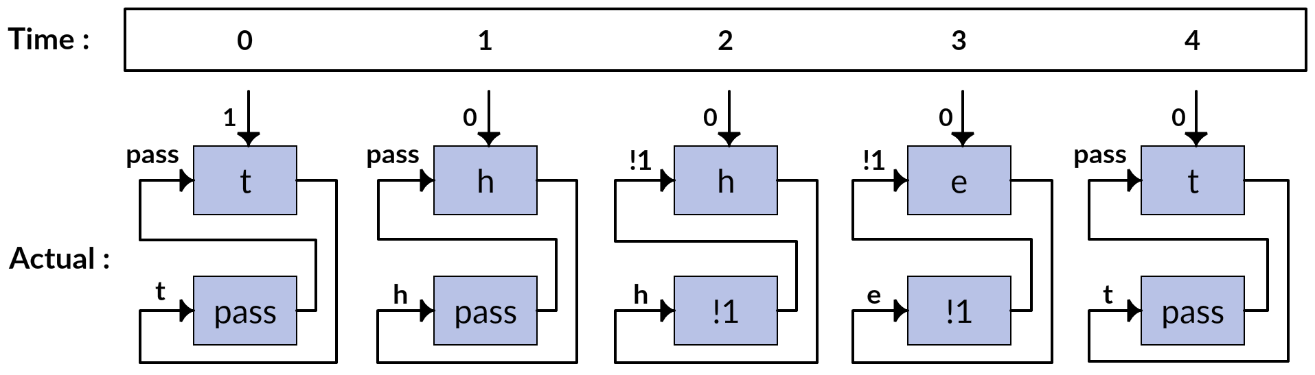
Figure 6: Graphical representation of trajectories in Table 2.

3.7 Philosopher system with slower choice input

In designing the controller and the new dynamics of the philosopher, one needs to take into account the fact that the controller needs one time step to compute its control input. During this step, no new input should arrive. In other words, the choice input should arrive slow enough so that it synchronises with the arrival of the control input.

Keeping this in mind, we redesign the choice type to include a $\bot$ (read “bottom”) input that denotes the absence of choice. This lifted input choice domain

$$B_{\bot}=\mbox{$\{\bot\}$}\cup B$$

is now used to define the absence of input ($\bot$) or the presence of a choice input (either 0 or 1). We let the variable $b_{\bot}$ range over elements of $B_{\bot}$.

A new deterministic and transparent philosopher system $S$ (for slower) may then be defined as follows:

$$S=\mbox{$\langle a:X=\mbox{\it Act},a^{0}:X^{0}=\mbox{$\{{\sf{t}}\}$},(b_{\bot},c):U=B_{\bot}\times\mbox{\it Cmd},f_{S}\rangle$}$$

where $f_{S}:\mbox{\it Act}\times B_{\bot}\times\mbox{\it Cmd}\rightarrow\mbox{\it Act}$ is defined as

$$f_{S}(a,\bot,c) =a$$ (5)

$$f_{S}(a,b,c) =f_{M}(a,b,c),\ \mbox{otherwise}$$ (6)

Expanding the definition of $f_{M}$, we have

$$f_{S}(a,\bot,c) =a$$ (7)

$$f_{S}(a,b,{\sf{pass}}) =f_{P}(a,b)$$ (8)

$$f_{S}(a,\_,!\;b) =f_{P}(a,b)$$ (9)

If the choice input is $\bot$, the model $S$’s next state stays the same as the previous state, irrespective of the control input. Otherwise, the $S$’s behaviour is just like that of $M$: its next state is governed by the function $f_{M}$, which expands to the two clauses $f_{P}$ shown above.

3.8 System $T$: feedback control system solving the 1 Diner problem

The new composite system $T=C\times_{{\cal{I}}_{T}}S$ is defined with respect to the interconnect

$${\cal{I}}_{T}=\mbox{$\{(C.c,S.a,C.a,S.b_{\bot},S.c)|S.a=C.a,C.c=S.c\}$}$$

which is similar to the interconnect ${\cal{I}}_{R}$. We write $a$, $b_{\bot}$ and $c$ to denote $S.a$, $S.b_{\bot}$ and $S.c$.

In composing the system $S$ with the controller $C$, we assume that the choice input to the philosopher alternates between absent ($\bot$) and present (0 or 1). In other words, we assume that the choices are expressed slowly (with one cycle of inactivity in between) so that the controller has enough time to compute the control input. (Another way of achieving this is to drive the philosopher system with a clock of time period of two units.)

Example Consider the prefix of $T$’s behaviour on an input choice stream with prefix

$$\langle\bot,\ 1,\ \bot,\ 0,\ \bot,\ 0,\ \bot,\ 0,\ \bot,\ 1,\ \bot\rangle$$

Note that each choice input is interspersed with one $\bot$. The trace of $T$ shown in Table 3 demonstrates that the discrepancy in Table 2 is avoided.

Table 3: Computations of state variables in the system $T$ for the prefix $\langle\bot,\ 1,\ \bot,\ 0,\ \bot,\ 0,\ \bot,\ 0,\ \bot,\ 1,\ \bot\rangle$ of choice $u_{P^{\prime}}$.

$t$	$b_{\bot}$	desired	$a$	$c$
0	$\bot$	t	t	pass
1	1	t	t	pass
2	$\bot$	h	h	pass
3	0	h	h	!1
4	$\bot$	e	e	!1
5	0	e	e	pass
6	$\bot$	e	e	pass
7	0	e	e	pass
8	$\bot$	e	e	pass
9	1	e	e	pass
10	$\bot$	t	t	pass

3.9 Dynamics of the 1 Diner system

We examine dynamics of the composite system $T$ with philosopher subsystem $S$ interconnected with the controller $C$. Let $t\in\mathbb{N_{0}}$ denote the number of clock cycles of the global clock whose time period is assumed one unit. We assume that each subsystem takes one clock cycle to compute its next state given its input. We also assume that $b_{\bot}[t]=\bot$ if $t$ is even, and equal to choice $b$, where $b\in B$, if $t$ is odd.

The following system of equations define the dynamics of the 1 Diner system:

Initialisation:

$$a[0] ={\sf{t}}$$

$$b_{\bot}[0] =\bot$$

$$c[0] =pass$$

Next state functions:

$$a[t+1] =f_{S}(a[t],b_{\bot}[t],c[t])$$ (10)

$$c[t+1] =g_{C}(a[t])$$ (11)

Using the prime (’) notation, these may be rewritten as

$$a^{\prime} =f_{S}(a,b_{\bot},c)$$ (12)

$$c^{\prime} =g_{C}(a)$$ (13)

Given $b_{\bot}[0]=\bot$, it is easy to verify that

$$c[1] =c[0]={\sf{pass}}$$

$$a[1] =a[0]={\sf{t}}$$

Tracing the dynamics from time $2t$ to $2t+3$, we have:

$$a[2t+1] =f_{S}(a[2t],b_{\bot}[2t],c[2t])$$

$$=f_{S}(a[2t],\bot,c[2t]) b_{\bot}[2t]$$ From the defn. of

$$=a[2t]$$ (14)

$$c[2t+1] =g_{C}(a[2t])$$

$$=g_{C}(a[2t+1])$$ From Eq. 14 (15)

$$a[2t+2] =f_{S}(a[2t+1],b_{\bot}[2t+1],c[2t+1])$$

$$=f_{S}(a[2t+1],b[2t+1],c[2t+1]) b_{\bot}[2t+1]$$ From the defn. of (16)

$$c[2t+2] =g_{C}(a[2t+1])$$

$$=g_{C}(a[2t])$$ From Eq. 14

$$=c[2t+1]$$ (17)

$$a[2t+3] =f_{S}(a[2t+2],b_{\bot}[2t+2],c[2t+2])$$

$$=f_{S}(a[2t+2],\bot,c[2t+2])$$

$$=a[2t+2] f_{S}$$ From the defn. of (Eq. 7) (18)

$$=f_{S}(a[2t+1],b[2t+1],c[2t+1])$$ From Eq. 16 (19)

$$c[2t+3] =g_{C}(a[2t+2])$$

$$=g_{C}(a[2t+3])$$ From Eq. 18

From this we conclude the following, for $t\in\mathbb{N_{0}}$.

$$a[2t+3] =f_{S}(a[2t+1],b[2t+1],c[2t+1])$$ Ref. Eq. 19

$$b_{\bot}[2t+1] =b[2t+1]$$ Assumption

$$c[2t+1] =g_{C}(a[2t+1])$$ Ref. Eq. 15

3.10 Simplified dynamics by polling

The dynamics may be reduced to a simpler system of equations if we consider polling the system once every two clock cycles. We define a step to be two clock cycles, with the $i$th step corresponding to the $2i+1$ clock cycle. The relation between the new set of variables $[a_{2},b_{2},c_{2}]$ and the previous variables is shown below:

$$a_{2}[0] =a[1]={\sf{t}}$$

$$c_{2}[0] =c[1]={\sf{pass}}$$

$$b_{2}[0] =b_{\bot}[1]=b[1]$$

and

$$a_{2}[i] =a[2i+1]$$

$$b_{2}[i] =b_{\bot}[2i+1]$$

$$c_{2}[i] =c[2i+1]$$

To continue using the old variables, we abuse notation and write $a$ etc., to refer to $a_{2}$, etc. Thus the polled dynamics, indexed over steps $i$ reduces to:

$$a[0] ={\sf{t}}$$

$$c[0] ={\sf{pass}}$$

$$c[i] =g_{C}(a[i])$$

$$a[i+1] =f_{S}(a[i],b[i],c[i])$$

We simplify notation further by making the indexing with $i$ implicit and writing $a$ to mean $a[i]$ and $a^{\prime}$ to denote $a[i+1]$. Thus

$$a^{0} =t$$ (20)

$$c^{0} ={\sf{pass}}$$ (21)

$$c =g_{C}(a)$$ (22)

$$a^{\prime} =f_{S}(a,b,c)$$ (23)

Equations 20 to 23 completely capture the ’polled dynamics’ of the composite system consisting of the controller with the philosopher. Note that $\bot$ is no longer relevant to the polled dynamics.

3.11 Correctness of the solution for the 1 Diner problem

Proposition 3.2.

Consider the composite system $T=C\times_{{\cal{I}}}S$ working under the assumption that choice inputs arrive only at odd cycles. Then, the system correctly implements the starvation freedom constraint of the 1 Diner problem which states that the philosopher doesn’t remain hungry forever. It defers to the philosopher’s own choice (stay at the same state or switch to the next) when the philosopher is not hungry.

Proof.

The result follows from the following propositions, which are simple consequences of the polled dynamics:

1. if $a={\sf{h}}$, then $a^{\prime}={\sf{e}}$.

2. if $a\neq{\sf{h}}$, then $a^{\prime}=f_{P}(a,b)$.

∎

4 N Dining Philosophers with Centralised control

We now look at the Generalised Dining Philosophers problem. We are given a graph $G=\mbox{$\langle V,E\rangle$}$, with $|V|=N$ and with each of the N vertices representing a philosopher and $E$ representing an undirected, adjacency relation between vertices. The vertices are identified by integers from 1 to N.

Each of the N philosophers are identical and modeled as the instances of the system $S$ described in the 1 Diner case. These N vertices are all connected to a single controller (called the hub) which reads the activity status of each of the philosophers and then computes a control input for that philosopher. The control input, along with the choice input to each philosopher computes the next state of that philosopher.

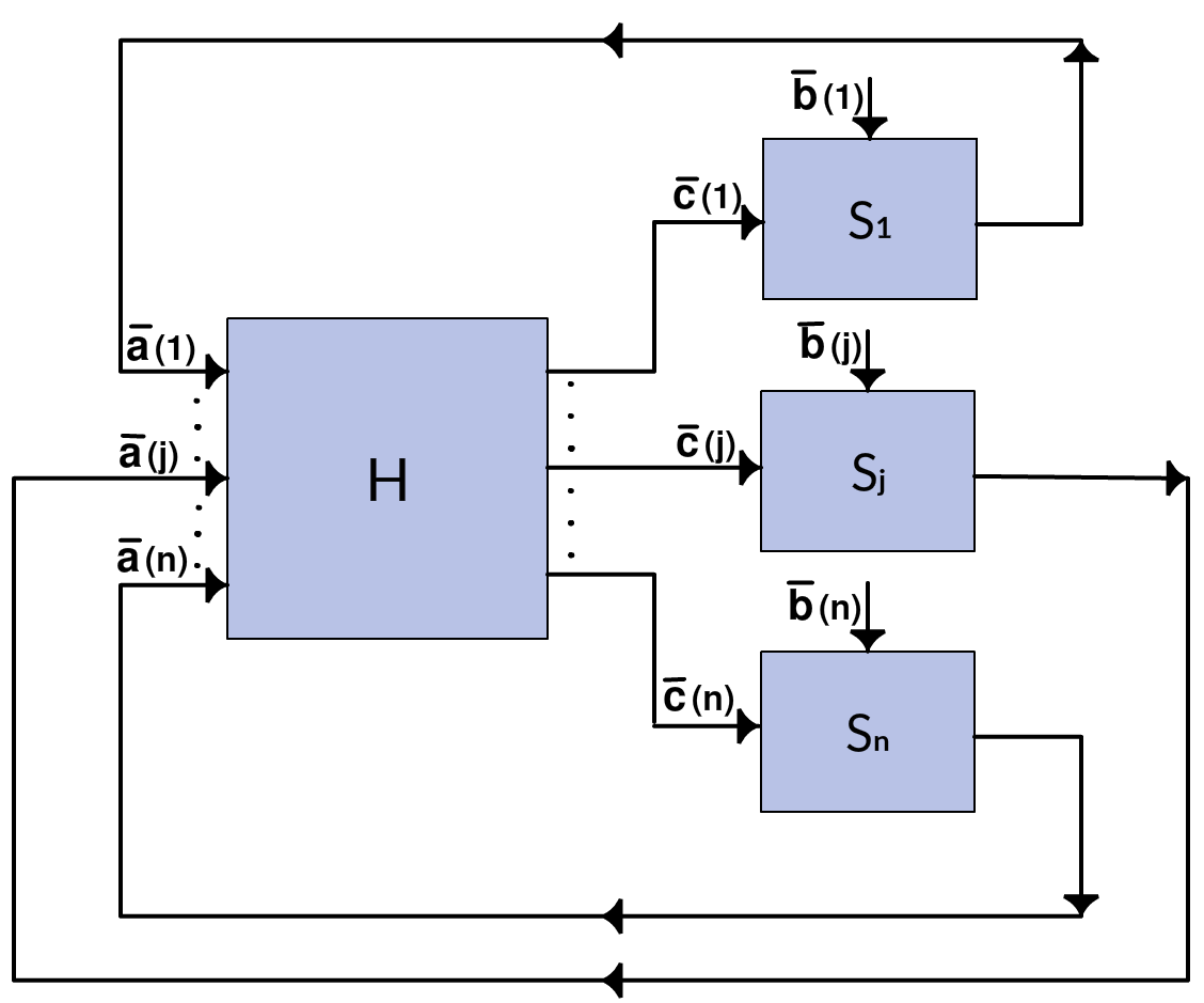
Figure 7: Wiring diagram describing the architecture of centralised controller.

Notation 4.1.

Identifiers $j,k,l\in V$ denote vertices.

An activity map $\overline{a}:V\rightarrow A$ maps vertices to their status, whether hungry, eating or thinking.

A choice map $\overline{b}:V\rightarrow B$ maps to each vertex a choice value.

A maybe choice map $\overline{m}:V\rightarrow B_{\bot}$ maps to each vertex a maybe choice value (nil or a choice).

A command map $\overline{c}:V\rightarrow\mbox{\it Cmd}$ maps to each vertex a command.

If $v$ is a constant, then $\overline{v}$ denotes a function that maps every vertex to the constant $v$.

The data structures and notation used in the solution are described below:

1. $G=(V,E)$, the graph of vertices $V$ and their adjacency relation $E$. $G$ is part of the hub’s internal state. $G$ is constant throughout the problem.

   We write $\mbox{$\{j,k\}$}\in E$, or $E(j,k)$ to denote that there is an undirected edge between $j$ and $k$ in $G$. We write $E(j)$ to denote the set of all neighbours of $j$.

2. $\overline{a}:V\rightarrow\mbox{$\{{\sf{t}},{\sf{h}},{\sf{e}}\}$}$, an activity map. This is input to the hub controller.

3. $D:(j,k)\in E\rightarrow\mbox{$\{j,k\}$}$, is a directed relation derived from $E$. $D$ is called a dominance map or priority map. For each edge $\{j,k\}$ of $E$ it returns the source of the edge. The element $\mbox{$\{j,k\}$}\mapsto j$ of $D$ is indicated $j\mapsto k$ ($j$ dominates $k$) whereas $\mbox{$\{j,k\}$}\mapsto k$ is indicated $k\mapsto j$ ($j$ is dominated by $k$). If $\mbox{$\{j,k\}$}\in E$, then exactly one of $j\mapsto k\in D$ or $k\mapsto j\in D$ is true.

   $D(j)$ is the set of vertices dominated by $j$ in $D$ and is called the set of subordinates of $j$. $D^{-1}(j)$ denotes the set of vertices that dominate $j$ in $D$ and is called the set of dominators of $j$.

4. $\mbox{\it top}(D)$, the set of maximal elements of $D$. $\mbox{\it top}(D)(j)$ means that $j\in\mbox{\it top}(D)$. This is a derived internal state of the hub controller.

5. $\overline{c}:V\rightarrow\mbox{\it Cmd}$, the command map. This is part of the internal state of the hub controller and also its output.

Additional Notation

Let $s\in A$, and $\overline{a}$ be an activity map. Then $E_{s}(\overline{a})(j)$ denotes the set of neighbours of $j$ whose activity value is $s$. Likewise $D_{s}(\overline{a})(j)$ denotes the set of vertices in the subordinate set of $j$ whose activity status is $s$.

4.1 Informal introduction to the control algorithm

Initially, at cycle $t=0$, all vertices in $G=(V,E)$ are thinking, so $\overline{a}[0]=\overline{{\sf{t}}}$. Also, $D[0]$ is $D^{0}$, $\mbox{\it top}(D)[0]=\{j\ |\ D^{0}(j)=E(j)\}$ and $\overline{c}[0]=\overline{{\sf{pass}}}$.

Upon reading the activity map, the controller performs the following sequence of computations:

1. (Step 1): Updates $D$ so that (a) a vertex that is eating is dominated by all its neighbours, and (b) any hungry vertex also dominates its thinking neighbours.

2. (Step 2): Computes top, the set of top vertices.

3. (Step 3): Computes the new control input for each philosopher vertex: A thinking or eating vertex is allowed to pass. A hungry vertex that is at the top and has no eating neighbours is commanded to switch to eating. Otherwise, the vertex is commanded to stay hungry.

4.2 Formal structure of the Hub controller

The centralised or hub controller is a deterministic system $H=\mbox{$\langle X,X^{0},U,f,Y,h\rangle$}$, where

1. $X_{H}=(E\rightarrow\mathbb{B})\times(V\rightarrow\mbox{\it Cmd})$ is the cross product of the set of all priority maps derived from $E$ with the set of command maps on the vertices of $G$. Each element $x_{H}:X_{H}$ is a tuple $(D,\overline{c})$ consisting of a priority map $D$ and a command map $\overline{c}$.

2. $X^{0}_{H}=(D^{0},\overline{c}^{0})$ where $D^{0}(\mbox{$\{j,k\}$})=j\mapsto k$ if $j>k$ and $k\mapsto j$ otherwise for $\mbox{$\{j,k\}$}\in E$, and $\overline{c}^{0}(j)=\overline{{\sf{pass}}}$. Note that $D^{0}$ is acyclic.

3. $U_{H}$ is the set of activity maps. $\overline{a}:U_{H}$ represents the activity map that is input to the hub $H$.

4. $f_{H}:X,U\rightarrow X$ takes a priority map $D$, a command map $\overline{c}$, and an activity map $\overline{a}$ as input and returns a new priority map $D^{\prime}$ and a new command map.

   $f_{H}((D,\overline{c}),\overline{a})=(D^{\prime},g_{H}(D^{\prime},\overline{a}))$ where

   $$D^{\prime} =d_{H}(D,\overline{a})$$ (24)

   $$d_{H}(D,\overline{a}) \stackrel{{\scriptstyle{\sf def}}}{{=}}\mbox{$\{d_{H}(d,\overline{a})\ |\ d\in D\}$}$$ (25)

   $$d_{H}(j\mapsto k,\overline{a}) \stackrel{{\scriptstyle{\sf def}}}{{=}}(k\mapsto j),\quad\mbox{if $\overline{a}(j)={\sf{e}}$}$$ (26)

   $$\stackrel{{\scriptstyle{\sf def}}}{{=}}(k\mapsto j),\quad\mbox{if $\overline{a}(j)={\sf{t}}$\ and\ $\overline{a}(k)={\sf{h}}$}$$ (27)

   $$\stackrel{{\scriptstyle{\sf def}}}{{=}}(j\mapsto k),\quad\mbox{otherwise}$$ (28)

   Note that the symbol $d_{H}$ is overloaded to work on a directed edge as well as a priority map. $d_{H}$ implements the updating of the priority map $D$ to $D^{\prime}$ mentioned in (Step 1) above. The function $g_{H}$ computes the command map (Step 3). The command is pass if $j$ is either eating or thinking. If $j$ is hungry, then the command is !1if $j$ is ready, i.e., it is hungry, at the top (Step 2), and its neighbours are not eating. Otherwise, the command is !0.

   $$g_{H}(D,\overline{a})(j) \stackrel{{\scriptstyle{\sf def}}}{{=}}{\sf{pass}},\quad\mbox{if $\overline{a}(j)\in\mbox{$\{{\sf{t}},{\sf{e}}\}$}$}$$ (29)

   $$\stackrel{{\scriptstyle{\sf def}}}{{=}}{\sf{!1}},\quad\mbox{if $\mbox{\it ready}(D,\overline{a})(j)$}$$ (30)

   $$\stackrel{{\scriptstyle{\sf def}}}{{=}}{\sf{!0}},\quad\mbox{otherwise}$$ (31)

   $$\mbox{\it ready}(D,\overline{a})(j)\stackrel{{\scriptstyle{\sf def}}}{{=}}{\sf{true}},\quad\mbox{if } \overline{a}(j)={\sf{h}}\ \land$$ (32)

   $$j\in\mbox{\it top}(D)\ \land$$

   $$\forall k\in E(j):\ \overline{a}(k)\neq{\sf{e}}$$

   $$\mbox{\it top}(D) \stackrel{{\scriptstyle{\sf def}}}{{=}}\mbox{$\{j\in V\|\forall k\in E(j):j\mapsto k\}$}$$ (33)

5. $Y_{H}=V\rightarrow\mbox{\it Cmd}$: The output is a command map.

6. $h_{H}:X_{H}\rightarrow Y_{H}$ simply projects the command map from its state: $h_{H}(D,\overline{c})\stackrel{{\scriptstyle{\sf def}}}{{=}}\overline{c}$.

Note that an existing priority map $D$ when combined with the activity map results in a new priority map $D^{\prime}$. The new map $D^{\prime}$ is then passed to $g_{H}$ in order to compute the command map.

The first important property concerns the priority map update function.

Lemma 4.1 ($d_{H}$ is idempotent).

$d_{H}(D,\overline{a})=d_{H}(d_{H}(D,\overline{a}),\overline{a})$.

Proof.

The proof is a simple consequence of the definition of $d_{H}$. ∎

4.3 Composing the hub controller with the Philosophers

Consider the interconnect ${\cal{I}}$ between the hub $H$ and the $N$ philosopher instances $s_{j}$, $1\leq j\leq N$.

$${\cal{I}}\subseteq X_{H}\times U_{H}\times\Pi_{j=1}^{N}s_{j}.X\times s_{j}.U$$

that connects the output of each philosopher to the input of the hub, and connects the output of the hub to control input of the corresponding philosopher.

$${\cal{I}}= \{(x_{H},u_{H},s_{1}.x,s_{1}.u\ldots s_{n}.x,s_{n}.u)\ |$$

$$u_{H}(j)=h_{S}(s_{j}.x)\ \land\ h_{H}(x_{H})(j)=s_{j}.u,$$

$$1\leq j\leq N\}$$

The composite N Diners system is the product of the N+1 systems.

We assume that the composite system is synchronous and driven by a global clock. At time $i$, the activity map $\overline{a}[i]$ holds the $j$th philosopher’s activity at $\overline{a}[i](j)$. All the philosophers make their choice inputs at the same instant and the choice inputs alternate with the $\bot$ inputs. Without loss of generality, we assume that the controller takes one clock cycle to compute the control input.

The dynamics of the entire system may be described by the following system of equations:

Initialisation:

$$D[0] =D^{0}$$

$$\overline{c}[0] =\overline{{\sf{pass}}}$$

$$\overline{a}[0] =\overline{{\sf{t}}}$$

$$\overline{b_{\bot}}[0] =\overline{\bot}$$

Next state functions:

$$D[t+1] =d_{H}(D[t],\overline{a}[t])$$ (34)

$$\overline{c}[t+1] =g_{H}(D[t+1],\overline{a}[t])$$ (35)

$$\overline{a}[t+1] =f_{S}(\overline{a}[t],\overline{b_{\bot}}[t],\overline{c}[t])$$ (36)

Using the prime (’) notation, these may be rewritten as

$$D^{\prime} =d_{H}(D,\overline{a})$$ (37)

$$\overline{c}^{\prime} =g_{H}(D^{\prime},\overline{a})$$ (38)

$$\overline{a}^{\prime} =f_{S}(\overline{a},\overline{b_{\bot}},\overline{c})$$ (39)

The input to the system, the lifted choice map $\overline{b_{\bot}}$ alternates between $\overline{\bot}$ at time $2t$ and a choice map $\overline{b}$ at time $2t+1$.

Given $\overline{b_{\bot}}[0]=\overline{\bot}$, it is easy to verify that

$$D[1] =D[0]=D^{0}$$

$$\overline{c}[1] =\overline{c}[0]=\overline{{\sf{pass}}}$$

$$\overline{a}[1] =\overline{a}[0]=\overline{{\sf{t}}}$$

Tracing the dynamics from time $2t$ to $2t+3$, we have:

$$\overline{a}[2t+1] =f_{S}(\overline{a}[2t],\overline{b_{\bot}}[2t],\overline{c}[2t])$$

$$=f_{S}(\overline{a}[2t],\overline{\bot}[2t],\overline{c}[2t]) \overline{b_{\bot}}[2t]$$ From the defn. of

$$=\overline{a}[2t]$$ (40)

$$D[2t+1] =d_{H}(D[2t],\overline{a}[2t])$$ (41)

$$\overline{c}[2t+1] =g_{H}(D[2t+1],\overline{a}[2t])$$

$$=g_{H}(D[2t+1],\overline{a}[2t+1])$$ From Eq. 40 (42)

$$\overline{a}[2t+2] =f_{S}(\overline{a}[2t+1],\overline{b_{\bot}}[2t+1],\overline{c}[2t+1])$$

$$=f_{S}(\overline{a}[2t+1],\overline{b}[2t+1],\overline{c}[2t+1]) \overline{b_{\bot}}[2t+1]$$ From the defn. of (43)

$$D[2t+2] =d_{H}(D[2t+1],\overline{a}[2t+1])$$

$$=d_{H}(D[2t+1],\overline{a}[2t])$$ From Eq. 40

$$=D[2t+1] d_{H}$$ From 41 and idempotence of (44)

$$\overline{c}[2t+2] =g_{H}(D[2t+2],\overline{a}[2t+1])$$

$$=g_{H}(D[2t+2],\overline{a}[2t])$$ From Eq. 40

$$=g_{H}(D[2t+1],\overline{a}[2t])$$ From Eq. 44

$$=\overline{c}[2t+1]$$ (45)

$$\overline{a}[2t+3] =f_{S}(\overline{a}[2t+2],\overline{b_{\bot}}[2t+2],\overline{c}[2t+2])$$

$$=f_{S}(\overline{a}[2t],\overline{\bot},\overline{c}[2t+1])$$

$$=\overline{a}[2t+2] f_{S}$$ From the defn. of (Eq. 7) (46)

$$=f_{S}(\overline{a}[2t+1],\overline{b}[2t+1],\overline{c}[2t+1])$$ From Eq. 43 (47)

$$D[2t+3] =d_{H}(D[2t+2],\overline{a}[2t+2])$$

$$=d_{H}(D[2t+1],\overline{a}[2t+3])$$ From Eq. 46

$$\overline{c}[2t+3] =d_{H}(D[2t+3],\overline{a}[2t+2])$$

$$=d_{H}(D[2t+3],\overline{a}[2t+3])$$ From Eq. 46

From this we conclude the following, for $t\in\mathbb{N_{0}}$.

$$\overline{b_{\bot}}[2t+1] =\overline{b}[2t+1]$$ Assumption

$$\overline{c}[2t+1] =g_{H}(D[2t+1],\overline{a}[2t+1])$$ Ref. Eq. 51

$$\overline{a}[2t+3] =f_{S}(\overline{a}[2t+1],\overline{b}[2t+1],\overline{c}[2t+1])$$ Ref. Eq. 47

$$D[2t+3] =d_{H}(D[2t+1],\overline{a}[2t+3])$$ Ref. Eq. 46

4.4 Simplified dynamics by polling

The dynamics may be reduced to a simpler system of equations if we consider polling the system once every two clock cycles. We consider a new clock of twice the time period. The index variable $i$ refers to the newer clock. The relation between the new set of variables $[\overline{a}_{2},\overline{b}_{2},\overline{c}_{2},D_{2}]$ and the previous variables is shown below:

$$\overline{a}_{2}[i] =\overline{a}[2i+1]$$

$$\overline{b}_{2}[i] =\overline{b_{\bot}}[2i+1]$$

$$\overline{c}_{2}[i] =\overline{c}[2i+1]$$

$$D_{2}[i] =D[2i+1]$$

and

$$\overline{a}_{2}[0] =\overline{a}[1]=\overline{{\sf{t}}}$$

$$\overline{c}_{2}[0] =\overline{c}[1]=\overline{{\sf{pass}}}$$

$$D_{2}[0] =D[1]=D^{0}$$

$$\overline{b}_{2}[0] =\overline{b_{\bot}}[1]=\overline{b}[1]$$

To continue using the old variables, we abuse notation and write $\overline{a}$ etc., to refer to $\overline{a}_{2}$, etc. Thus the dynamics based on the new clock with ticks indicated by $i$ is shown below:

$$\overline{a}[0] =\overline{{\sf{t}}}$$

$$D[0] =D^{0}$$

$$\overline{c}[0] =\overline{{\sf{pass}}}$$

$$\overline{c}[i] =g_{H}(D[i],\overline{a}[i])$$

$$\overline{a}[i+1] =f_{S}(\overline{a}[i],\overline{b}[i],\overline{c}[i])$$

$$D[i+1] =d_{H}(D[i],\overline{a}[i+1])$$

We simplify notation further by making the indexing with $i$ implicit and writing $\overline{a}$ to mean $\overline{a}[i]$ and $\overline{a}^{\prime}$ to denote $\overline{a}[i+1]$. Thus

$$\overline{a}^{0} =\overline{{\sf{t}}}$$ (48)

$$\overline{c}^{0} =\overline{{\sf{pass}}}$$ (49)

$$D^{0} =\mbox{$\{j\mapsto k\ |\ E(j,k)\land j>k\}$}$$ (50)

$$\overline{c} =g_{H}(D,\overline{a})$$ (51)

$$\overline{a}^{\prime} =f_{S}(\overline{a},\overline{b},\overline{c})$$ (52)

$$D^{\prime} =d_{H}(D,\overline{a}^{\prime})$$ (53)

Equations 48 to 53 completely capture the ’polled dynamics’ of the composite system consisting of the hub controller with the N Diners. This dynamics is obtained by polling all odd instances of the clock, which is precisely when and only when the choice input is present. With the polled dynamics, we are no longer concerned with $\bot$ as as a choice input.

It is worth comparing the polled dynamics with the basic clocked dynamics of Eqs. 37 to 39. Note, in particular, the invariant that relates $\overline{a}$, $\overline{c}$ and $D$ in Eq. 51 of the polled dynamics. There is no such invariant in the basic clocked dynamics. Equation 52 of the polled dynamics may be seen as a specialisation of the corresponding Eq. 39 of the basic clocked dynamics. However, while Eq. 53 of the polled dynamics relates $D^{\prime}$ ($D$ in the next step) with $D$ and $\overline{a}^{\prime}$, its counterpart Eq. 37 in the basic clocked dynamics relates $D^{\prime}$ ($D$ in the next cycle) with $D$ and $\overline{a}$.

4.5 Asynchronous interpretation of the dynamics

It is worth noting that the equations we obtained in the polled dynamics of the system can be interpreted as asynchronous evolution of the philosopher system. A careful examination of the equations yields temporal dependencies between the computations of the variables involved in the systems. Consider the polled equations, consisting of indexed variables $\overline{a}$, $\overline{c}$ and $D$:

$$\overline{a}[0] =\overline{{\sf{t}}}$$

$$D[0] =D^{0}$$

$$\overline{c}[i] =g_{H}(D[i],\overline{a}[i])$$

$$\overline{a}[i+1] =f_{S}(\overline{a}[i],\overline{b}[i],\overline{c}[i])$$

$$D[i+1] =d_{H}(D[i],\overline{a}[i+1])$$

The asynchronous nature of the system dynamics tells us that the $i^{th}$ value of $\overline{c}$ requires the $i^{th}$ values of $\overline{a}$ and $D$ to be computed before its computation happens, and so on. This implicitly talks about the temporal dependency of the $i^{th}$ value of $\overline{c}$ on the $i^{th}$ values of $\overline{a}$ and $D$. Similarly, the $(i+1)^{th}$ value of $\overline{a}$ depends on the $i^{th}$ values of $\overline{a}$, $\overline{c}$ and $D$, and the $(i+1)^{th}$ value of $D$ depends on the $i^{th}$ value of $D$ and the $(i+1)^{th}$ value of $\overline{a}$. Note that they only talk about the temporal dependencies between variable calculations, and do not talk about the clock cycles, nor when the values are computed in physical time. The following figure depicts the dependencies between the variables.

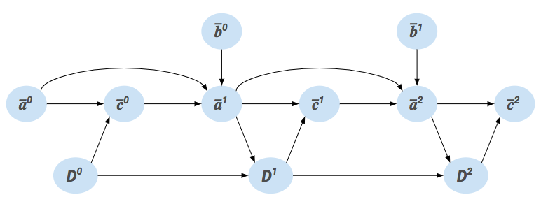
Figure 8: Dependencies between $\overline{a}$, $\overline{c}$ and $D$, along with input $\overline{b}$, shown for three calculations.

4.6 Basic properties of asynchronous dynamics

In the next several lemmas, we study the asynchronous (or polled) dynamics in detail. All of these are simple consequences of the functions $g_{H}$ and $f_{S}$. The first of several lemmas in this effort assures us that the asynchronous dynamics obeys the laws governing the dynamics of basic philosopher activity:

Lemma 4.2 (Asynchronous Dynamics).

Let $k\in V$. The dynamics satisfies the following:

1. If $\overline{a}(k)={\sf{t}}$, then $\overline{a}^{\prime}(k)\in\mbox{$\{{\sf{t}},{\sf{h}}\}$}$.

2. If $\overline{a}(k)={\sf{h}}$, then $\overline{a}^{\prime}(k)\in\mbox{$\{{\sf{h}},{\sf{e}}\}$}$.

3. If $\overline{a}(k)={\sf{e}}$, then $\overline{a}^{\prime}(k)\in\mbox{$\{{\sf{e}},{\sf{t}}\}$}$.

Proof.

This is a consequence of the dynamics $\overline{a}^{\prime}=f_{S}(\overline{a},\overline{b},\overline{c})$ and simply substituting the definitions of $\overline{c}$ and the value of $\overline{a}(k)$. We show the case when $\overline{a}(k)={\sf{t}}$. The others are similar.

$$\overline{a}^{\prime}(k) =f_{S}(\overline{a},\overline{b},\overline{c})(k)$$

$$=f_{S}({\sf{t}},\overline{b}(k),\overline{c}(k))$$

$$=f_{S}({\sf{t}},\overline{b}(k),g_{H}(D,\overline{a})(k))$$

$$=f_{S}({\sf{t}},\overline{b}(k),{\sf{pass}}) g_{H}$$ From the defn. of (Eq. 29)

$$=f_{P}({\sf{t}},\overline{b}(k)) f_{S}$$ From the defn. of (Eq. 8)

$$={\sf{t}}, \overline{b}(k)=0$$ if , or

$$={\sf{h}}, \overline{b}(k)=1$$ if

∎

The next lemma invests meaning to the phrase “priority map”. If $j$ has higher priority than a hungry vertex $k$, irrespective of whether $j$ stays hungry or switches to eating, in the next step, $k$ will continue to wait in the hungry state.

Lemma 4.3 (Priority map).

If $j\mapsto k\in D$ and $\overline{a}(k)={\sf{h}}$, then $\overline{a}^{\prime}(k)={\sf{h}}$.

Proof.

$$\overline{a}^{\prime}(k) =f_{S}({\sf{h}},\overline{b}(k),\overline{c}(k))$$

$$=f_{S}({\sf{h}},\overline{b}(k),g_{H}(D,\overline{a})(k))$$

$$=f_{S}({\sf{h}},\overline{b}(k),{\sf{!0}}) \mbox{\it ready}(D,\overline{a})(k)$$ Since is false

$$=f_{P}({\sf{h}},0) f_{S}$$ From the defn. of (Eq. 9)

$$={\sf{h}} f_{P}$$ From the defn. of (Eq. 3)

∎

The next lemma states that a hungry vertex with an eating neighbour stays hungry in the next step, irrespective of the eating vertex finishing eating in the next step or not. This lemma drives the safety invariant (described later) that ensures that no two adjacent vertices eat at the same time.

Lemma 4.4 (Continue to be hungry if neighbour eating).

If $E(j,k)$, $\overline{a}(j)={\sf{h}}$ and $\overline{a}(k)={\sf{e}}$ then $\overline{a}^{\prime}(j)={\sf{h}}$.

Proof.

$$\overline{a}^{\prime}(j) =f_{S}(\overline{a}(j),\overline{b}(j),\overline{c}(j))$$

$$=f_{S}({\sf{h}},\overline{b}(j),g_{H}(D,\overline{a})(j))$$

$$=f_{S}({\sf{h}},\overline{b}(j),{\sf{!0}}) \mbox{\it ready}(D,\overline{a})(j)$$ Since is false

$$=f_{P}({\sf{h}},0) f_{S}$$ From the defn. of (Eq. 9)

$$={\sf{h}} f_{P}$$ From the defn. of (Eq. 3)

∎

4.7 Safety and other invariants

Theorem 4.1.

The dynamics of the composition of the N philosophers with the hub controller satisfies the following invariants:

1. Eaters are sinks: If $\overline{a}(k)={\sf{e}}$ and $E(j,k)$, then $D(j,k)$.

2. Hungry dominate thinkers: If $\overline{a}(j)={\sf{h}}$ and $\overline{a}(k)={\sf{t}}$, and $E(j,k)$, then $D(j,k)$.

3. Safety: $\mbox{\it safe}(E,\overline{a})$: $\overline{a}(j)={\sf{e}}$ and $E(j,k)$ implies $\overline{a}(k)\neq{\sf{e}}$.

Proof.

The proof is by induction on $i$.

1. Eaters are sinks:

   The base case is vacuously true since $\overline{a}^{0}=\overline{{\sf{t}}}$.

   For the inductive case, assume $\overline{a}^{\prime}(k)={\sf{e}}$ and $E(j,k)$, we need to show that $D^{\prime}(j,k)$. This follows from the definition $D^{\prime}=d_{H}(D,\overline{a}^{\prime})$ and from the definition of $d_{H}$ (clause 26).

2. Hungry dominate thinkers:

   The proof of this claim is similar to that of the previous claim.

   The base case is vacuously true since $\overline{a}^{0}=\overline{{\sf{t}}}$ (there are no hungry nodes).

   For the inductive case, assume $\overline{a}^{\prime}(j)={\sf{h}}$ and $E(j,k)$ and $\overline{a}^{\prime}(k)={\sf{h}}$, we need to show that $D^{\prime}(j,k)$. Now, $D^{\prime}=d_{H}(D,\overline{a}^{\prime})$. From the definition of $d_{H}$ (clause 27), it follows that $j\mapsto k\in D^{\prime}$, i.e., $D^{\prime}(j,k)$.

3. Safety:

   The base case is trivially true since $\overline{a}^{0}=\overline{{\sf{t}}}$, i.e., all vertices are thinking.

   For the inductive case, we wish to show that $\mbox{\it safe}(E,\overline{a})$ implies $\mbox{\it safe}(E,\overline{a}^{\prime})$, where

   $$\overline{a}^{\prime}=f_{P}(\overline{a},\overline{b},\overline{c})$$

   Let $E(j,k)$. Let $\overline{a}^{\prime}(j)={\sf{e}}$. In each case, we prove that $\overline{a}^{\prime}(k)\neq{\sf{e}}$.

   1. $\overline{a}(j)={\sf{t}}$: By Lemma 4.2, $\overline{a}^{\prime}(j)\neq{\sf{e}}$. This violates the assumption that $\overline{a}^{\prime}(j)={\sf{e}}$.

   2. $\overline{a}(j)={\sf{e}}$: There are three cases:

      1. $\overline{a}(k)={\sf{t}}$: Again, by Lemma 4.2, $\overline{a}^{\prime}(k)\neq{\sf{e}}$.

      2. $\overline{a}(k)={\sf{h}}$: $\overline{c}=g_{H}(D,\overline{a})$. $k$ is hungry and it has an eating neighbour $j$. Hence $\overline{c}(k)={\sf{!0}}$. Now

         $$\overline{a}^{\prime}(k) =f_{S}(\overline{a}(k),\overline{b}(k),\overline{c}(k))$$

         $$\overline{a}^{\prime}(k) =f_{S}(\overline{a}(k),\overline{b}(k),{\sf{!0}})$$

         $$\overline{a}^{\prime}(k) =f_{P}(\overline{a}(k),0)$$

         $$=\overline{a}(k)$$

         $$={\sf{h}}$$

         Thus $\overline{a}^{\prime}(k)\neq{\sf{e}}$.

      3. $\overline{a}(k)={\sf{e}}$: This is ruled out by the induction hypothesis because $\overline{a}$ is safe.

   3. $\overline{a}(j)={\sf{h}}$: Again, there are three cases:

      1. $\overline{a}(k)={\sf{t}}$: $\overline{a}^{\prime}(k)\neq{\sf{e}}$ follows from Lemma 4.2.

      2. $\overline{a}(k)={\sf{h}}$: There are two cases:

         1. $j\mapsto k\in D$: From Lemma 4.3, $\overline{a}^{\prime}(k)\neq{\sf{e}}$.

         2. $k\mapsto j\in D$: By identical reasoning, $\overline{a}^{\prime}(j)\neq{\sf{e}}$, which contradicts the assumption that $\overline{a}^{\prime}(j)={\sf{e}}$.

      3. $\overline{a}(k)={\sf{e}}$: By the induction hypothesis (eaters are sinks) applied to $D$ and the fact that $E(j,k)$, it follows that $j\mapsto k\in D$. From Lemma 4.4, it follows that $\overline{a}^{\prime}(j)\neq{\sf{e}}$, which contradicts the assumption that $\overline{a}^{\prime}(j)={\sf{e}}$.

∎

4.8 Starvation freedom

Starvation-freedom means that every hungry vertex eventually eats. The argument for starvation freedom is built over the several lemmas.

The first of these asserts a central property of the priority map, that it is acyclic.

Lemma 4.5 (Priority Map is acyclic).

$D$ is acyclic.

Proof.

The proof is by induction on $i$.

The base case is true because $D^{0}$ is acyclic by construction.

For the inductive case, we need to show that $D^{\prime}$ is acyclic. Assume, for the sake of deriving a contradiction, that $D^{\prime}$ has a cycle. Since $D^{\prime}=d_{H}(D,\overline{a}^{\prime})$ and $D$ is acyclic by the induction hypothesis, the cycle in $D^{\prime}$ must involve an edge $d^{\prime}$ in $D^{\prime}$ but not in $D$.

$d^{\prime}$ is an edge $k\mapsto j$. There are two possibilities based on the first two clauses of the definition of $d_{H}$:

1. $\overline{a}^{\prime}(j)={\sf{e}}$: In that case by Theorem 4.1 1, $j$ is a sink in $D^{\prime}$. If $d^{\prime}$ is part of a cycle in $D^{\prime}$, then $j$ is part of that cycle, but since $j$ is a sink, it can not participate in any cycle. Contradiction.

2. $\overline{a}^{\prime}(j)={\sf{t}}$ and $\overline{a}^{\prime}(k)={\sf{h}}$: Since $k\mapsto j$ is an edge in $D^{\prime}$, there is a path

   $$j\rightarrow l_{1}\mapsto\ldots l_{m}\mapsto l_{m+1}\ldots\mapsto k$$

   in $D^{\prime}$.

   Then it must be the case that for some $m$, $\overline{a}^{\prime}(l_{m})={\sf{t}}$ and $\overline{a}^{\prime}(l_{m+1})={\sf{h}}$ and $D^{\prime}(l_{m},l_{m+1})$. But by Theorem 4.1 2, $D^{\prime}(l_{m+1},l_{m})$. We can not have both $D^{\prime}(l_{m},l_{m+1})$ and $D^{\prime}(l_{m+1},l_{m})$. Contradiction.

∎

The next set of lemmas demonstrate how the function $d_{H}$ transforms the subordinate and dominator set of a hungry vertex that is left unchanged in the next step.

Lemma 4.6 (Monotonicity of subordinate set and Anti-monotonicity of dominator set).

Let $\overline{a}(j)={\sf{h}}$ and $\overline{a}^{\prime}(j)={\sf{h}}$,

1. Subordinate set monotonicity: $D(j)\subseteq D^{\prime}(j)$.

2. Dominator set anti-monotonicity: $D^{\prime-1}(j)\subseteq D^{-1}(j)$.

Proof.

The proof relies on examining the clauses of the definition $d_{H}$:

1. Subordinate set monotonicity: Let $D(j,k)$. We wish to prove that $D^{\prime}(j,k)$.

   Now, $D^{\prime}=d_{H}(D,\overline{a}^{\prime})$. Consider $d_{H}(j\mapsto k,\overline{a}^{\prime})$: Since $\overline{a}^{\prime}(j)={\sf{h}}$, it follows, from the third clause of the definition of $d_{H}$ that $j\mapsto k\in D^{\prime}$, i.e., $D^{\prime}(j,k)$.

2. Dominator set anti-monotonicity: Let $D^{\prime-1}(j,k)$. We wish to show that $D^{-1}(j,k)$. $D^{\prime-1}(j,k)$ means that $D^{\prime}(k,j)$. Similarly, $D^{-1}(j,k)$ means that $D(k,j)$.

   Thus we are given that $D^{\prime}(k,j)$ and we need to show that $D(k,j)$. Now, $D^{\prime}=d_{H}(D,\overline{a}^{\prime})$ and $\overline{a}^{\prime}(k)={\sf{h}}=\overline{a}^{\prime}(j)$. We reason backwards with the definition of $d_{H}$. We are given something in the range $D^{\prime}$ of $d_{H}$, we reason why it also exists in the domain $D$. In the definition of $d_{H}$, only the last clause is applicable, which leaves the edge unchanged. Since $D^{\prime}(k,j)$, it follows that $D(k,j)$.

∎

As a corollary, a hungry vertex that is top and continues to be hungry in the next step also continues to be a top vertex.

Corollary 4.1 (Top continues).

Given that $\overline{a}(j)={\sf{h}}=\overline{a}^{\prime}(j)$, and $\mbox{\it top}(D)(j)$, it follows that $\mbox{\it top}(D^{\prime})(j)$.

Proof.

From Lemma 4.6, part 2, $D^{\prime-1}(j)\subseteq D^{-1}(j)$. Since $\mbox{\it top}(D)(j)$, it means that $D^{-1}(j)=\emptyset$. It follows that $D^{\prime-1}(j)=\emptyset$, i.e., $\mbox{\it top}(D^{\prime})(j)$. ∎

The next lemma examines the set of eating neighbours of a top hungry vertex after a step that leaves the vertex hungry and at the top.

Lemma 4.7 (No new eating neighbours if top continues).

Let $\overline{a}(j)={\sf{h}}=\overline{a}^{\prime}(j)$ and $\mbox{\it top}(D)(j)$. Then $D^{\prime}_{{\sf{e}}}(j)\subseteq D_{{\sf{e}}}(j)$.

Proof.

For the sake of deriving a contradiction, assume that $D^{\prime}_{{\sf{e}}}(j)\not\subseteq D_{{\sf{e}}}(j)$.

Then there is some vertex $k$ such that $k\in D^{\prime}_{{\sf{e}}}(j)$ and $k\not\in D_{{\sf{e}}}(j)$. Since $k\in D^{\prime}_{{\sf{e}}}(j)$, $k$ is a neighbour of $j$. We are given that $\overline{a}^{\prime}(k)={\sf{e}}$ and $\overline{a}(k)\neq{\sf{e}}$.

This leaves us with two possibilities:

1. $\overline{a}(k)={\sf{t}}$: Then, by Lemma 4.2, $k$’s activity cannot be ${\sf{e}}$ in the next step. Therefore $k\not\in E^{\prime}_{{\sf{e}}}(j)$. Contradiction.

2. $\overline{a}(k)={\sf{h}}$: Since $j$ is top in $D$, $j\mapsto k\in D$. Then by Lemma 4.3, $\overline{a}^{\prime}(k)={\sf{h}}$, so $k\not\in E^{\prime}_{{\sf{e}}}(j)$. Contradiction again.

∎

The next lemma generalises the second part of the previous lemma and relates the closure of the dominator set of a hungry vertex going from one step to the next.

Lemma 4.8 (Transitive closure of the dominator set does not grow).

If $\overline{a}(j)={\sf{h}}=\overline{a}^{\prime}(j)$, then $D^{\prime-1+}(j)\subseteq D^{-1+}(j)$.

Proof.

If $\overline{a}(j)={\sf{h}}$, let $P(j)$ denotes the length of the longest path from a top vertex in $D$ to $j$. Note that $P$ is well defined since $D$ is acyclic. Also, if $k\mapsto j\in D$, then, from Theorem 4.1, parts 1 (Eaters are sinks) and 2 (Hungry dominate thinkers), $\overline{a}(k)={\sf{h}}$ and therefore $P(k)$ is well-defined, and furthermore, $P(k)<P(j)$.

The proof is by induction on $P(j)$.

Base case: $P(j)=0$. This implies that $j$ is a top vertex in $D$ and therefore $D^{-1}(j)=\emptyset$. Then from Corollary 4.1, $j$ is a top vertex in $D^{\prime}$ that is hungry. Thus $D^{-1}(j)=\emptyset$ and the result follows.

Inductive case: $P(j)>0$. Now

$$D^{-1+}(j)=D^{-1}(j)\cup\mbox{$\{D^{-1+}(k)\ |\ k\in D^{-1}(j)\}$}$$

and, similarly

$$D^{\prime-1+}(j)=D^{\prime-1}(j)\cup\mbox{$\{D^{\prime-1+}(k)\ |\ k\in D^{\prime-1}(j)\}$}$$

Let $l\in D^{\prime-1+}(j)$. There are two cases:

1. $l\in D^{\prime-1}(j)$: From Lemma 4.6, part 2, it follows that $l\in D^{-1}(j)$ and hence $l\in D^{-1+}(j)$.

2. $l\in D^{\prime-1+}(k)$ for some $k\in D^{\prime-1}(j)$: Then, by another application of Lemma 4.6, part 2, it follows that $k\in D^{-1}(j)$. That is $k\mapsto j\in D$. That means that $P(k)<P(j)$.

   Applying the induction hypothesis on $k$, we have $D^{\prime-1+}(k)\subseteq D^{-1+}(k)$. Hence $l\in D^{-1+}(k)$. From this it follows that $l\in D^{-1+}(j)$.

∎

We now prove that the N Diners with centralised controller exhibits starvation freedom.

Theorem 4.2 (starvation freedom).

The system of N Dining Philosophers meets the following starvation freedom properties:

1. Eater eventually finishes: If $j$ is eating, then $j$ will eventually finish eating.

2. Top eventually eats: If $j$ is a hungry top vertex, then $j$ will eventually start eating.

3. Hungry eventually tops: If $j$ is a hungry vertex that is not top, then $j$ will eventually become a top vertex.

From the above three properties, one may conclude that a hungry vertex eventually eats.

The proof of this theorem hinges on defining an appropriate set of metrics on each behaviour of the Dining Philosophers problem.

Proof.

We define a set of metrics that map a hungry or eating vertex $j$ to a natural number:

1. Let $W_{{\sf{e}}}:V\rightarrow\mathbb{N_{0}}\rightarrow\mathbb{N_{0}}$ be defined as follows:

   $W_{{\sf{e}}}(j)[i]=0$ if $\overline{a}(j)\neq{\sf{e}}$, otherwise $W_{{\sf{e}}}(j)[i]$ is equal to the number of steps remaining before $j$ finishes eating. Clearly, $W_{{\sf{e}}}(j)$ is positive as long as $j$ eats and $0$ otherwise.

2. Let $W_{{\sf{top}}}:V\rightarrow\mathbb{N_{0}}\rightarrow\mathbb{N_{0}}$ be defined as follows:

   $$W_{{\sf{top}}}(j)[i] =\Sigma_{k\in D_{{\sf{e}}}[i](j)}W_{{\sf{e}}}(k)[i],\quad\mbox{if $\mbox{\it top}(D,j)$ and $\overline{a}(j)={\sf{h}}$}$$

   Note that $W_{{\sf{top}}}(j)[i]$ is positive as long as $j$ is a hungry top vertex that is not ready, and $0$ otherwise.

3. If $\overline{a}(j)={\sf{h}}$:

   $$W_{{\sf{h}}}(j) \stackrel{{\scriptstyle{\sf def}}}{{=}}[|D^{-1+}(j)|,$$

   $$\quad\quad\Sigma\mbox{$\{W_{{\sf{top}}}(k)\ |\ k\in D^{-1+}(j)\ \land\mbox{\it top}(D)(k)\}$}]$$

$W_{{\sf{h}}}$ is a pair $[v_{1},v_{2}]$. $W_{{\sf{h}}}$ is well defined since $D$ is acyclic. The ordering is lexicographic: $[v^{\prime}_{1},v^{\prime}_{2}]<[v_{1},v_{2}]$ iff $v^{\prime}_{1}<v_{1}$ or $v^{\prime}_{1}=v_{1}$ and $v^{\prime}_{2}<v_{2}$. $D^{-1+}(j)$ denotes the transitive closure of $\{j\}$ with respect to $D^{-1}$. If $j$ is is not at the top, then $D^{-1+}(j)\neq\emptyset$ and therefore $v_{1}>0$. If $j$ is at the top then $W_{{\sf{h}}}(j)=[0,0]$.

We prove the following:

1. $W_{{\sf{e}}}$ is a decreasing function: If $\overline{a}(j)={\sf{e}}=\overline{a}^{\prime}(j)$, then $W^{\prime}_{{\sf{e}}}(j)<W_{{\sf{e}}}(j)$. The proof is obvious from the definition of $W_{{\sf{e}}}$.

2. $W_{{\sf{top}}}$ is a decreasing function: If $\overline{a}(j)={\sf{h}}=\overline{a}^{\prime}(j)$, then $W_{{\sf{top}}}^{\prime}(j)<W_{{\sf{top}}}(j)$. Since $j$ is a hungry top vertex in $D$ and hungry in $D^{\prime}$, it follows from Corollary 4.1 (Top continues) that $j$ is a top vertex in $D^{\prime}$.

   $$W^{\prime}_{{\sf{top}}}(j) =\Sigma_{k\in D^{\prime}_{{\sf{e}}}(j)}W_{{\sf{e}}}^{\prime}(k)$$

   $$<\Sigma_{k\in D_{{\sf{e}}}(j)}W_{{\sf{e}}}(k)$$

   $$=W_{{\sf{top}}}(j)$$

   The penultimate inequality holds because of the following two reasons: From Lemma 4.7, $D^{\prime}_{{\sf{e}}}(j)\subseteq D_{{\sf{e}}}(j)$. Second, from the definition of $W_{{\sf{e}}}$, for each $k\in D^{\prime}_{{\sf{e}}}$, $W^{\prime}_{{\sf{e}}}(k)<W_{{\sf{e}}}(k)$.

   The last step holds because $j$ is top in $D$.

3. $W_{{\sf{h}}}$ is a decreasing function: If $\overline{a}(j)={\sf{h}}=\overline{a}^{\prime}(j)$, $j$ is not top in $D$, then $W^{\prime}_{{\sf{h}}}(j)<W_{{\sf{h}}}(j)$.

   To prove this, consider the definition of $W_{{\sf{h}}}(j)$:

   $$W^{\prime}_{{\sf{h}}}(j) =[|D^{\prime-1+}(j)|,$$

   $$\quad\quad\Sigma\mbox{$\{W^{\prime}_{{\sf{top}}}(k)\ |\ k\in D^{\prime-1+}(j)\ \land\mbox{\it top}(D^{\prime})(k)\}$}]$$

   From Lemma 4.8, $D^{\prime-1+}(j)\subseteq D^{-1+}(j)$. There are two cases:

   1. $D^{\prime-1+}(j)\subset D^{-1+}(j)$: Clearly, $W^{\prime}_{{\sf{h}}}(j)<W_{{\sf{h}}}(j)$.

   2. $D^{\prime-1+}(j)=D^{-1+}(j)$: Again, there are two cases:

      1. $D^{-1+}(j)=\emptyset$: then $j$ is a hungry top vertex $D$. This violates the assumption that $j$ is not top in $D$.

      2. $D^{-1+}(j)\neq\emptyset$: Then, for each top vertex $k$ in $D^{-1+}(j)$ and $D^{\prime-1+}(j)$, $k$ is in the domain of $W_{{\sf{top}}}$ and $W^{\prime}_{{\sf{top}}}$. Furthermore, from part 2, $W^{\prime}_{{\sf{top}}}(k)<W_{{\sf{top}}}(k)$. The result follows: $W^{\prime}_{{\sf{h}}}(j)<W_{{\sf{h}}}(j)$.

∎

5 Distributed Solution to the N Diners problem

In the distributed version of N Diners, each philosopher continues to be connected to other philosophers adjacent to it according to $E$, but there is no central hub controller. Usually the problem is stated as trying to devise a protocol amongst the philosophers that ensures that the safety and starvation freedom conditions are met. The notion of devising a protocol is best interpreted as designing a collection of systems and their composition.

5.1 Architecture and key idea

The centralised architecture employed the global maps $\overline{a}$, $\overline{b}$, $\overline{c}$ and $D$. While the first three map a vertex $j$ to a value (activity, choice input, or control) the last maps an edge $\{j,k\}$ to one of the vertices $j$ or $k$.

The key to devising a solution for the distributed case is to start with the graph $G=\mbox{$\langle V,E\rangle$}$ and consider its distributed representation. The edge relation $E$ is now distributed across the vertex set $V$. Let $\alpha_{j}$ denote the size of the set of neighbours $E(j)$ of $j$. We assume that the neighbourhood $E(j)$ is arbitrarily ordered as a vector $\vec{E_{j}}$ indexed from $1$ to $\alpha_{j}$. Let $j$ and $k$ be distinct vertices in $V$ and let $\mbox{$\{j,k\}$}\in E$. Furthermore, let the neighbourhoods of $j$ and $k$ be ordered such that $k$ is the $m$th neighbour of $j$ and $j$ is the $n$th neighbour of $k$. Then, by definition, $\vec{E_{j}}(m)=k$ and $\vec{E_{k}}(n)=j$.

In addition, with each vertex $j$ is associated a philosopher system $S_{j}$ and a local controller system $L_{j}$. The philosopher system $S_{j}$ is an instance of the system $S$ defined in Section 3.7. In designing the local controllers, the guiding principle is to distribute the state of the centralised controller to $N$ local controllers. The state of the centralised controller consists of the directed graph $D$ that maps each edge in $E$ to its dominating endpoint and the map $\overline{c}:V\longrightarrow\mbox{\it Cmd}$ which is also the output of the hub controller.

The information about the direction of an edge $\{j,k\}$ is distributed across two dominance vectors $\vec{d_{j}}$ and $\vec{d_{k}}$. Both are boolean vectors indexed from 1 to $\alpha_{j}$ and $\alpha_{k}$, respectively. Assume that $k=\vec{E_{j}}(m)$ and $j=\vec{E_{k}}(n)$. Then, the value of $D(\mbox{$\{j,k\}$})$ is encoded in $\vec{d_{j}}$ and $\vec{d_{k}}$ as follows: If $D(\mbox{$\{j,k\}$})=j$ then $\vec{d_{j}}(m)={\sf{true}}$ and $\vec{d_{k}}(n)={\sf{false}}$. If $D(\mbox{$\{j,k\}$})=k$, then $\vec{d_{j}}(m)={\sf{false}}$ and $\vec{d_{k}}(n)={\sf{true}}$.

In the next subsection we define the local controller as a Tabuada system.

5.2 Local controller system for a vertex $j$

The controller system $L_{j}$ has $\alpha_{j}+1$ input ports of type $A$ which are indexed $0$ to $\alpha_{j}$. The output of $L_{j}$ is of type Cmd.

The local controller $L_{j}$ is a Tabuada system

$$L_{j}=\mbox{$\langle X,X^{0},U,f,Y,h\rangle$}$$

where

1. $X=([1..\alpha_{j}]\longrightarrow\mathbb{B})\times\mbox{\it Cmd}$. Each element of $X$ is a tuple $(\vec{d_{j}},c_{j})$ consisting of a dominance vector $\vec{d_{j}}$ indexed $1$ to $\alpha_{j}$ and a command value $c_{j}$. $\vec{d_{j}}(m)={\sf{true}}$ means that there is a directed edge from $j$ to its $m$th neighbour $k$; ${\sf{false}}$ means that there is an edge from its $m$th neighbour to $j$.

2. $X^{0}$ is defined as follows: $X^{0}=\mbox{$\langle\vec{d^{0}_{j}},c^{0}_{j}\rangle$}$ where $c^{0}_{j}={\sf{pass}}$ and $\vec{d^{0}_{j}}(m)={\sf{true}}$ if $\vec{E_{j}}(m)=k$ and $j>k$, ${\sf{false}}$ otherwise. In other words, there is an edge from $j$ to $k$ if $j>k$.

3. $U=[0..\alpha_{j}]\longrightarrow A$: We denote the input to $L_{j}$ as a vector $\vec{a_{j}}$, the activities of all the neighbours of the $j^{th}$ philosopher, including its own activity. $\vec{a_{j}}(m)$ denotes the value of the $m$th input port.

4. $f_{L}:X,U\longrightarrow X$ defines the dynamics of the controller and is given below.

5. $Y=\mbox{\it Cmd}$, and

6. $h:X\rightarrow Y$ and $h(\vec{d_{j}},c_{j})=c_{j}$. The output of the controller $L_{j}$ is denoted $c_{j}$.

The function $f_{L}$ takes a dominance vector $\vec{d}$ of length $M$, a command $c$ and an activity vector $\vec{a}$ of length $M+1$ and returns a pair consisting of a new dominance vector $\vec{d^{\prime}}$ of length $M$ and a new command $c^{\prime}$. $f_{L}$ first computes the new dominance vector $\vec{d^{\prime}}$ using the function $d_{L}$. The result $\vec{d^{\prime}}$ is then passed along with $\vec{a}$ to the function $g_{L}$, which computes the new command value $c^{\prime}$. The functions $f_{L}$ and $d_{L}$ are defined below:

$$f_{L}((\vec{d},c),\vec{a})=(\vec{d^{\prime}},c^{\prime})\quad\mbox{where}$$

$$\vec{d^{\prime}} =\vec{d_{L}}(\vec{d},\vec{a}),\ \mbox{and}$$ (54)

$$c^{\prime} =g_{L}(\vec{d^{\prime}},\vec{a})$$ (55)

$$\vec{d_{L}}(\vec{d},\vec{a})(m) \stackrel{{\scriptstyle{\sf def}}}{{=}}d_{L}(\vec{d}(m),\vec{a}(0),\vec{a}(m))\quad\mbox{where $m\in[1..M]$}$$ (56)

$d_{L}(d,a_{0},a)$ is defined as

$$d_{L}(d,{\sf{t}},{\sf{t}}) =d$$ (57)

$$d_{L}(d,{\sf{t}},{\sf{h}}) ={\sf{false}}$$ (58)

$$d_{L}(d,{\sf{t}},{\sf{e}}) ={\sf{true}}$$ (59)

$$d_{L}(d,{\sf{h}},{\sf{e}}) ={\sf{true}}$$ (60)

$$d_{L}(d,{\sf{h}},{\sf{h}}) =d$$ (61)

$$d_{L}(d,{\sf{e}},{\sf{h}}) ={\sf{false}}$$ (62)

$$d_{L}(d,{\sf{e}},{\sf{t}}) ={\sf{false}}$$ (63)

$$d_{L}(d,{\sf{h}},{\sf{t}}) ={\sf{true}}$$ (64)

$$d_{L}(d,{\sf{e}},{\sf{e}}) =d$$ (65)

$d_{L}(\vec{d}(m),\vec{a}(0),\vec{a}(m))$ takes the $m$th component of a dominance vector $\vec{d}$ and computes the new value based on the activity values at the $0$th and $m$th input ports of the controller.

The function $g_{L}$ takes a dominance vector $\vec{d}$ of size $M$ and an activity vector $\vec{a}$ of size $M+1$ and computes a command. It is defined as follows:

$$g_{L}(\vec{d},\vec{a}) \stackrel{{\scriptstyle{\sf def}}}{{=}}{\sf{pass}},\quad\quad\mbox{if $\vec{a}(0)\in\mbox{$\{{\sf{t}},{\sf{e}}\}$}$}$$

$$\stackrel{{\scriptstyle{\sf def}}}{{=}}{\sf{!1}},\quad\mbox{if $\mbox{\it ready}_{L}(\vec{d},\vec{a})={\sf{true}}$}$$

$$\stackrel{{\scriptstyle{\sf def}}}{{=}}{\sf{!0}},\quad\mbox{otherwise}$$

$$\mbox{\it ready}_{L}(\vec{d},\vec{a}) \stackrel{{\scriptstyle{\sf def}}}{{=}}{\sf{true}},\quad\mbox{if $\vec{a}(0)={\sf{h}}$ and $\mbox{\it top}_{L}(\vec{d})$ and $\forall m\in[1..M]:\ \vec{a}(m)\neq{\sf{e}}$}$$

$$\stackrel{{\scriptstyle{\sf def}}}{{=}}{\sf{false}},\quad\mbox{otherwise}$$

$$\mbox{\it top}_{L}(\vec{d}) \stackrel{{\scriptstyle{\sf def}}}{{=}}{\sf{true}},\quad\mbox{if $\forall m\in[1..M]:\vec{d}(m)={\sf{true}}$}$$

$$\stackrel{{\scriptstyle{\sf def}}}{{=}}{\sf{false}},\quad\mbox{otherwise}$$

Now we can write down the equations that define the asynchronous dynamics of the philosopher system. Consider any arbitrary philosopher $j$ and its local controller $L_{j}$:

$$a_{j}^{0} ={\sf{t}}$$ (66)

$$\mbox{For $m\in[1..\alpha_{j}]:$}\quad\vec{d_{j}}^{0}(m) ={\sf{true}},\quad\mbox{if $\vec{E_{j}}(m)=k$ and $j>k$}$$ (67)

$$={\sf{false}},\quad\mbox{otherwise}$$

$$c_{j} =g_{L}(\vec{d_{j}},\vec{a_{j}})$$ (68)

$$a_{j}^{\prime} =f_{S}(a_{j},b_{j},c_{j})$$ (69)

$$\vec{d_{j}}^{\prime} =d_{L}(\vec{d_{j}},\vec{a_{j}^{\prime}})$$ (70)

Note from equation 69 that the philosopher dynamics has not changed - it is the same as that of the centralised case. A close examination of the equations help us deduce that the dynamics we obtained in the distributed case are very much comparable to that of the centralised case. This identical nature of the dynamics form the foundation for the correctness proofs which follow later.

5.3 Wiring the local controllers and the philosophers

Each philosopher $S_{j}$ is defined as the instance of the system $S$ defined in Section 3.7. Let the choice input, control input and output of the philosopher system $S_{j}$ be denoted by the variables $S_{j}.c$, $S_{j}.b_{\bot}$ and $S_{j}.a$, respectively. The output of $L_{j}$ is fed as the control input to $S_{j}$. The output $S_{j}$ is fed as $0$th input of $L_{j}$. In addition, for each vertex $j$, if $k$ is the $m$th neighbour of $j$, i.e., $k=\vec{E_{j}}(m)$, then the output of $S_{k}$ is fed as the $m$th input to $L_{j}$. (See Fig. 9).

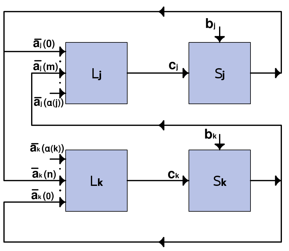
Figure 9: Wiring between the systems of adjacent philosophers $j$ and $k$ where $k$ and $j$ are respectively the $m$th and $n$th neighbour of each other.

The wiring between the $N$ philosopher systems and the $N$ local controllers is the interconnect relation ${\cal{I}}\subseteq\Pi_{j}S_{j}.X\times S_{j}.U\times L_{j}.X\times L_{j}.U$, $1\leq j\leq N$ defined via the following set of constraints:

1. $c_{j}=S_{j}.c$: The output of the local controller $L_{j}$ is equal to the control input of the philosopher system $S_{j}$.

2. $S_{j}.a=\vec{a_{j}}(0)$: the output of the philosopher $S_{j}$ is fed back as the input of the 0th input port of the local controller $L_{j}$.

3. $S_{k}.a=\vec{a_{j}}(m)$, where $1\leq m\leq\alpha_{j}$ and $k=\vec{E_{j}}(m)$: the output of the philosopher $S_{k}$ is connected as the input of the $m$th input port of the local controller $L_{j}$ where $k$ is the $m$th neighbour of $j$.

4. $\vec{d_{j}}(m)=\neg\vec{d_{k}}(n)$, where $k=\vec{E_{j}}(m)$ and $j=\vec{E_{k}}(n)$. The dominance vector at $j$ is compatible with the dominance vectors of the neighbours of $j$.

5.4 Correctness of the solution to the Distributed case

The correctness of the solution for the distributed case rests on the claim that under the same input sequence, the controllers and the philosopher outputs in the distributed and centralised cases are identical. This claim in turn depends on the fact that the centralised state may be reconstructed from the distributed state.

Theorem 5.1 (Correctness of Distributed Solution to N Diners).

Consider the sequence of lifted choice inputs fed to both the centralised and the distributed instances of an N Diners problem. We show that after equal number of computations, for each $j\in V$:

1. $\overline{a}(j)=a_{j}$: The output $\overline{a}(j)$ of the $j$th Philosopher in the centralised architecture is identical to the output $a_{j}$ of the $j$th Philosopher in the distributed architecture.

2. $\overline{c}(j)=c_{j}$: $\overline{c}(j)$, the $j$th output of hub controller in centralised architecture is identical to the output $c_{j}$ of the $j$th local controller in the distributed architecture.

3. For each $k\in E(j)$,

   1. $k=\vec{E_{j}}(m)$ for some $m\in[1..\alpha_{j}]$, and

   2. $j=\vec{E_{k}}(n)$ for some $n\in[1..\alpha_{k}]$, and

   3. $j\mapsto k\in D$ iff $\vec{d_{j}}(m)={\sf{true}}$ and $\vec{d_{k}}(n)={\sf{false}}$.

Proof.

Note that in the last clause it is enough to prove one direction (only if) since, if $k\in E(j)$ and $j\mapsto k\not\in D$ implies $k\mapsto j\in D$; the proof of this case is simply an instantiation of the theorem with $k$ instead of $j$.

The proof for the rest of the conditions is by induction on the number of computations.

For the base case, in the centralised architecture, the initial values for each vertex $j$ are $\overline{a}^{0}(j)={\sf{t}}$, $\overline{c}^{0}(j)={\sf{pass}}$, and for each $k\in E(j)$, $D^{0}(\mbox{$\{j,k\}$})$ is equal to $j$ if $j>k$, and $k$ otherwise.

In the distributed regime, the initial value $a_{j}$ of the output of Philosopher $S_{j}$ is ${\sf{t}}$ by definition of $S_{j}$. The initial value of the output $c_{j}$ of the local controller $L_{j}$ is ${\sf{pass}}$ by definition. Also, note that in the initial state $\vec{d_{j}}(m)={\sf{true}}$ iff $k=\vec{E_{j}}(m)$ and $j>k$, ${\sf{false}}$ otherwise.

Assume, for the sake of the induction hypothesis, the premises above are all true. We wish to show that

1. $\overline{a}^{\prime}(j)=a^{\prime}_{j}$

2. $\overline{c}^{\prime}(j)=c^{\prime}_{j}$

3. For each $k\in D^{\prime}(j)$,

   1. $k=\vec{E_{j}}(m)$ for some $m\in[1..\alpha_{j}]$, and

   2. $j=\vec{E_{k}}(n)$ for some $n\in[1..\alpha_{k}]$, and

   3. $j\mapsto k\in D^{\prime}$ iff $\vec{d^{\prime}_{j}}(m)={\sf{true}}$ and $\vec{d^{\prime}_{k}}(n)={\sf{false}}$.

We start with $D^{\prime}$. Suppose $j\mapsto k\in D^{\prime}$. We need to show that $\vec{d^{\prime}_{j}}(m)={\sf{true}}$ and $\vec{d^{\prime}_{k}}(n)={\sf{false}}$. Based on the definition of $d_{H}$, there are three cases:

1. Case 1 (clause 26 of $d_{H}$):

   $$\overline{a}(k)={\sf{e}}$$ (71)

   $$k\mapsto j\in D$$ (72)

   Note the substitution requires swapping $k$ and $j$ in clause 26.

   From the above two conditions, applying the inductive hypthothesis, we have

   $$\vec{d_{k}}(n) ={\sf{true}}$$ (73)

   $$\vec{d_{j}}(m) ={\sf{false}}$$ (74)

   $$a_{k} ={\sf{e}}$$ (75)

   $\vec{d^{\prime}_{j}}(m)$ may now be computed as follows:

   $$\vec{d^{\prime}_{j}}(m) =d_{L}(\vec{d_{j}}(m),\vec{a_{j}}(0),\vec{a_{j}}(m))$$

   $$=d_{L}({\sf{false}},a_{j},a_{k})$$

   $$=d_{L}({\sf{false}},a_{j},{\sf{e}})$$

   An inspection of the definition of $d_{L}$ reveals three cases that have ${\sf{e}}$ in the third argument: 59, 60, and 65. Of these, the last case is ruled out because of the safety property of the centralised solution; no two adjacent vertices eat at the same time. For each of the other two cases, $\vec{d^{\prime}_{j}}(m)$ yields ${\sf{true}}$.

   Computing $\vec{d^{\prime}_{k}}(n)$,

   $$\vec{d^{\prime}_{k}}(n) =d_{L}(\vec{d_{k}}(n),\vec{a_{k}}(0),\vec{a_{k}}(m))$$

   $$=d_{L}({\sf{true}},a_{k},a_{j})$$

   $$=d_{L}({\sf{true}},{\sf{e}},a_{j})$$

   A similar examination of cases 63, 62 allows us to conclude that $\vec{d^{\prime}_{k}}(n)={\sf{false}}$.

2. Case 2 (clause 27 of $d_{H}$):

   $$\overline{a}(k)={\sf{t}}$$ (76)

   $$\overline{a}(j)={\sf{h}}$$ (77)

   $$k\mapsto j\in D$$ (78)

   Note again that the substitution requires swapping $k$ and $j$, this time in clause 27.

   From the above conditions, applying the induction hypothesis,

   $$\vec{d_{k}}(n)={\sf{true}}$$ (79)

   $$\vec{d_{j}}(m)={\sf{false}}$$ (80)

   $$a_{k}={\sf{t}}$$ (81)

   $$a_{j}={\sf{h}}$$ (82)

   $\vec{d^{\prime}_{j}}(m)$ may now be computed as follows:

   $$\vec{d^{\prime}_{j}}(m) =d_{L}(\vec{d_{j}}(m),\vec{a_{j}}(0),\vec{a_{j}}(m))$$

   $$=d_{L}({\sf{false}},a_{j},a_{k})$$

   $$=d_{L}({\sf{false}},{\sf{h}},{\sf{t}})$$

   $$={\sf{true}}$$

   Computing $\vec{d^{\prime}_{k}}(n)$,

   $$\vec{d^{\prime}_{k}}(n) =d_{L}(\vec{d_{k}}(n),\vec{a_{k}}(0),\vec{a_{k}}(m))$$

   $$=d_{L}({\sf{true}},a_{k},a_{j})$$

   $$=d_{L}({\sf{true}},{\sf{t}},{\sf{h}})$$

   $$={\sf{false}}$$

3. Case 3: From clause 28 of $d_{H}$, it follows that

   $$j\mapsto k\in D$$ (83)

   $$\overline{a}(j)\neq{\sf{e}}$$ (84)

   $$\neg(\overline{a}(j)={\sf{t}}\ \mbox{and}\ \overline{a}(k)={\sf{h}})$$ (85)

   By the induction hypothesis

   $$\vec{d_{j}}(m)={\sf{true}}$$ (86)

   $$\vec{d_{k}}(n)={\sf{false}}$$ (87)

   $$a_{j}\neq{\sf{e}}$$ (88)

   $$\neg(a_{j}={\sf{t}}\ \mbox{and}\ a_{k}={\sf{h}})$$ (89)

   $\vec{d^{\prime}_{j}}(m)$ may now be computed as follows:

   $$\vec{d^{\prime}_{j}}(m) =d_{L}(\vec{d_{j}}(m),\vec{a_{j}}(0),\vec{a_{j}}(m))$$

   $$=d_{L}({\sf{true}},a_{j},a_{k})$$

   The conditions on $a_{j}$ and $a_{k}$ eliminate the possibilities 58, 62, 63, and 65 in the definition of $d_{L}$. Of the remaining five cases, three cases 59, 60 and 64 yield the value ${\sf{true}}$, while the remaining two cases (57 and 61) yield the value $\vec{d_{j}}(m)$, which by induction hypothesis, is also ${\sf{true}}$.

   $\vec{d^{\prime}_{k}}(n)$ may now be computed as follows:

   $$\vec{d^{\prime}_{k}}(n) =d_{L}(\vec{d_{k}}(n),\vec{a_{k}}(0),\vec{a_{k}}(m))$$

   $$=d_{L}({\sf{false}},a_{k},a_{j})$$

   Again, the condition $a_{j}\neq{\sf{e}}$ eliminates the possibilities 59, 60, 65 and 65 in the definition of $d_{L}$. Of the remaining six cases, the impossibility of the condition $a_{k}={\sf{h}}$ and $a_{j}={\sf{t}}$, eliminates the case 64.

   Of the remaining five cases, three of them, 58, 62 and 63 yield the value ${\sf{false}}$, while the remaining two cases (57 and 61) yield the value $\vec{d_{k}}(n)$, which by induction hypothesis, is also ${\sf{false}}$.

The next thing to prove is the claim $\overline{c}(j)=c_{j}$ for all computations. The proof is by induction: Verify that $\overline{c}^{0}(j)=c^{0}_{j}$ and $\overline{c}(j)=c_{j}$ implies $\overline{c}^{\prime}(j)=c^{\prime}_{j}$.

The proof proceeds by first showing that

$$j\in\mbox{\it top}(D)\ \mbox{iff}\ \mbox{\it top}_{L}(\vec{d_{j}})={\sf{true}}$$ (90)

$$\mbox{\it ready}(D,\overline{a})(j)\ \mbox{iff }\mbox{\it ready}_{L}(\vec{d_{j}},\vec{a_{j}})={\sf{true}}$$ (91)

$$g_{H}(D,\overline{a})(j) =g_{L}(\vec{d_{j}},\vec{a_{j}})$$ (92)

The proofs of each of these are straightforward and omitted.

Finally, in both the centralised and distributed architectures, the philosopher system instances are identical and hence they have the same dynamics, they both operate with identical initial conditions ($\overline{a}(j)=a_{j}={\sf{t}}$) and in each case the choice inputs are identical and the control inputs, which are outputs of the respective controllers, are identical as well ($\overline{c}(j)=c_{j}$ as proved above). From this, it follows that $\overline{a}(j)=a_{j}$ for all computations.

∎

This concludes our formal analysis of the Generalised N Diners problem and its solution for centralised and distributed scenarios.

6 Related Work

This section is in two parts: the first is a detailed comparison with Chandy and Misra’s solution, the second is a survey of several other approaches.

6.1 Comparison with Chandy and Misra solution

Chandy and Misra[6] provides the original statement and solution to the Generalised Dining Philosophers problem. There are several important points of comparison with their problem formulation and solution.

The first point of comparison is architecture: in brief, shared variables vs. modular interconnects. Chandy and Misra’s formulation of the problem identifies the division between a user program, which holds the state of the philosophers, and the os, which runs concurrently with the user and modifies variables shared with the user. Our formulation is based on formally defining the two main entities, the philosopher and the controller, as formal systems with clearly delineated boundaries and modular interactions between them. The idea of feedback control is explicit in the architecture, not in the shared variable approach.

Another advantage of the modular architecture that our solution affords is apparent when we move from the centralised solution to the distributed solution. In both cases, the definition of the philosopher remains exactly the same; additional interaction is achieved by wiring a local controller to each philosopher rather than a central controller. We make a reasonable assumption that the output of a philosopher is readable by its neighbours. In Chandy and Misra’s solution, the distributed solution relies on three shared boolean state variables per edge in the user: a boolean variable fork that resides with exactly one of the neighbours, its status clean or dirty, and a request token that resides with exactly one neighbour, adding up to $3|E|$ boolean variables. These variables are not distributed; they reside with the os, which still assumes the role of a central controller. In our solution, the distribution of philosopher’s and their control is evident. Variables are distributed across the vertices: each vertex $j$ with degree $j$ has $\alpha(j)+1$ input ports of type Act that read the neighbours’ plus self’s activity status. In addition, each local controller has, as a boolean vector $\vec{d}_{j}$ of length $\alpha(j)$ as part of its internal state, that keeps information about the direction of each edge with $j$ as an endpoint. A pleasant and useful property of this approach is that the centralised data structure $D$ may be reconstructed by the union of local data structures $\vec{d}$ at each vertex.

The second point of comparison is the algorithm and its impact on reasoning. Both approaches rely on maintaining the dominance graph $D$ as a partial order. As a result, in both approaches, if $j$ is hungry and has priority over $k$, then $j$ eats before $k$. In Chandy and Misra’s algorithm, however, $D$ is updated only when a hungry vertex transits to eating to ensure that eating vertices are sinks. In our solution, $D$ is updated to satisfy an additional condition that hungry vertices always dominate thinking vertices. This ensures two elegant properties of our algorithm, neither of which are true in Chandy and Misra: (a) a top vertex is also a maximal element of the partial order $D$, (b) a hungry vertex that is at the top remains so until it is ready, after which it starts eating. In Chandy and Misra’s algorithm, a vertex is at the top if it dominates only (all of its) hungry neighbours; it could still be dominated by a thinking neighbour. It is possible that a hungry top vertex is no longer at the top if a neighbouring thinking vertex becomes hungry (Table 4). This leads us to the third property that is true in our approach but not in Chandy and Misra’s: amongst two thinking neighbours $j$ and $k$, whichever gets hungry first gets to eat first.

Table 4: Example demonstrating two properties of Chandy and Misra’s algorithm: (a) a top hungry vertex no longer remains top, and (b) In step 3, Vertex 1, which was at the top, is hungry, but no longer at the top.

i	G	D	top	remarks
0	$\{1:{\sf{t}},2:{\sf{t}},3:{\sf{t}}\}$	$\{2\mapsto 1,3\mapsto 1\}$	$\{2,3\}$	initial
1	$\{1:{\sf{h}},2:{\sf{t}},3:{\sf{h}}\}$	ditto	$\{2,3\}$	$3$ at top
2	$\{1:{\sf{h}},2:{\sf{t}},3:{\sf{e}}\}$	$\{2\mapsto 1,1\mapsto 3\}$	$\{1,2\}$	$1$ is at the top
3	$\{1:{\sf{h}},2:{\sf{h}},3:{\sf{e}}\}$	ditto	$\{2\}$	$2$ is at the top, not $1$

6.2 Comparison with other related work

Literature on the Dining Philosophers problem is vast. Our very brief survey is slanted towards approaches that — explicitly or implicitly — address the modularity and control aspects of the problem and its solution. [28] surveys the effectiveness of different solutions against various complexity metrics like response time and communication complexity. Here, we leave out complexity theoretic considerations and works that explore probabilistic and many other variants of the problem.

6.3 Early works

Dijkstra’s Dining Philosophers problem was formulated for the five philosophers seated in a circle. Dijsktra later generalized it to N philosophers. Lynch[22] generalised the problem to a graph consisting of an arbitrary number of philosophers connected via edges depicting resource sharing constraints. Lynch also introduced the notion of an interface description of systems captured via external behaviour, i.e., execution sequences of automata. This idea was popularized by Ramadge and Wonham[29] who advocated that behaviour be specified in terms of language-theoretic properties. They also introduce the idea of control to affect behaviour.

Chandy and Misra[5, 6] propose the idea of a dynamic acyclic graph via edge reversals to solve the problem of fair resolution of contention, which ensures progress. This is done by maintaining an ordering on philosophers contending for a resource. The approach’s usefulness and generality is demonstrated by their introduction of the Drinking Philosophers problem as a generalisation of the Dining Philosophers problem. In the Drinking Philosophers problem, each philosopher is allowed to possess a subset of a set of resources (drinks) and two adjacent philosophers are allowed to drink at the same time as long as they drink from different bottles. Welch and Lynch[37, 23] present a modular approach to the Dining and Drinking Philosopher problems by abstracting the Dining Philosophers system as an I/O automaton. Their paper, however, does not invoke the notion of control. Rhee[30] considers a variety of resource allocation problems, include dining philosophers with modularity and the ability to use arbitrary resource allocation algorithms as subroutines as a means to compare the efficiency of different solutions. In this approach, resource managers are attached to each resource, which is similar in spirit to the local controllers idea.

6.4 Other approaches

Sidhu et al.[32] discuss a distributed solution to a generalised version of the dining philosophers problem. By putting additional constraints and modifying the problem, like the fixed order in which a philosopher can occupy the forks available to him and the fixed number of forks he needs to occupy to start eating, they show that the solution is deadlock free and robust. The deadlock-free condition is assured by showing that the death of any philosopher possessing a few forks does not lead to the failure of the whole network, but instead disables the functioning of only a finite number of philosophers. In this paper, the philosophers require multiple (>2) forks to start eating, and the whole solution is based on forks and their constraints. Also, this paper discusses the additional possibility of the philosophers dying when in possession of a few forks, which is not there in our paper.

Weidman et al.[36] discuss an algorithm for the distributed dynamic resource allocation problem, which is based on the solution to the dining philosophers problem. Their version of the dining philosophers problem is dynamic in nature, in that the philosophers are allowed to add and delete themselves from the group of philosophers who are thinking or eating. They can also add and delete resources from their resource requirements. The state space is modified based on the new actions added: adding/deleting self, or adding/deleting a resource. The main difference from our solution is the extra option available to the philosophers to add/delete themselves from the group of philosophers, as well as add/delete the resources available to them. The state space available to the philosophers is also expanded because of those extra options - there are total 7 states possible now - whereas our solution allows only 3 possible states (thinking, hungry and eating). Also, the notion of a ’controller’ is absent here - the philosophers’ state changes happen depending on the neighbours and the resources availability, but there is no single controller which decides it.

Zhan et al.[39] propose a mathematical model for solving the original version of the dining philosophers problem by modeling the possession of the chopsticks by the philosophers as an adjacency matrix. They talk about the various states of the matrix which can result in a deadlock, and a solution is designed in Java using semaphores which is proven to be deadlock free, and is claimed to be highly efficient in terms of resource usability.

Awerbuch et al.[3] propose a deterministic solution to the dining philosophers problem that is based on the idea of a "distributed queue", which is used to ensure the safety property. The collection of philosophers operate in an asynchronous message-driven environment. They heavily focus on optimizing the "response time" of the system to each job (in other words, the philosopher) to make it polynomial in nature. In our solution, we do not talk about the response time and instead we focus on the modularity of the solution, which is not considered in this solution.

A distributed algorithm for the dining philosophers algorithm has been implemented by Haiyan[14] in Agda, a proof checker based on Martin-Lof’s type theory. A precedence graph is maintained in this solution where directed edges represent precedences between pairs of potentially conflicting philosophers, which is the same idea as the priority graph we have in our solution. But unlike our solution, they also have chopsticks modelled as part of the solution in Agda.

Hoover et al.[17] describe a fully distributed self-stabilizing solution to the dining philosophers problem. An interleaved semantics is assumed where only one philosopher at a time changes its state, like the asynchronous dynamics in our solution. They use a token based system, where tokens keeps circling the ring of philosophers, and the possession of a token enables the philosopher to eat. The algorithm begins with a potentially illegal state with multiple tokens, and later converges to a legal state with just one token. Our solution do not have this self-stabilization property, as we do not have any "illegal" state in our system at any point of time.

The dining philosophers solution mentioned in the work by Keane et al.[18] uses a generic graph model like the generalized problem: edges between processes which can conflict in critical section access. Modification of arrows between the nodes happens during entry and exit from the critical section. They do not focus on aspects like modularity or equational reasoning, but on solving a new synchronization problem (called GRASP).

Cargill[4] proposes a solution which is distributed in the sense that synchronization and communication is limited to the immediate neighbourhood of each philosopher without a central mechanism, and is robust in the sense that the failure of a philosopher only affects its immediate neighbourhood. Unlike our solution, forks are modelled as part of their solution.

You et al.[38] solve the Distributed Dining Philosophers problem, which is the same as the Generalized Dining Philosophers problem, using category theory. The phases of philosophers, priority of philosophers, state-transitions etc. are modelled as different categories and semantics of the problem are explained. They also make use the graph representation of the priorities we have used in our paper.

Nesterenko et al.[27] present a solution to the dining philosophers problem that tolerates malicious crashes, where the failed process behaves arbitrarily and ceases all operations. They talk about the use of stabilization - which allows the program to recover from an arbitrary state - and crash failure locality - which ensures that the crash of a process affects only a finite other processes - in the optimality of their solution.

Chang[7] in his solution tries to decentralise Dijkstra’s solution to the dining philosophers problem by making use of message passing and access tokens in a distributed system. The solution does not use any global variables, and there is no notion of ’controllers’ in the solution like we have in ours. Forks are made use of in the solution.

Datta et al.[8] considers the mobile philosophers problem in which a dynamic network exists where both philosophers and resources can join/leave the network at any time, and the philosophers can connect/disconnect to/from any point in the network. The philosopher is allowed to move around a ring of resources, making requests to the resources in the process. The solution they propose is self-stabilizing and asynchronous.

6.5 Supervisory control

The idea of using feedback (or supervisory) control to solve the Dining Philosophers program is not new. Miremadi et al.[25] demonstrate how to automatically synthesise a supervisory controller using Binary Decision Diagrams. Their paper uses Hoare composition but does not describe the synthesised controller, nor do they attempt to prove why their solution is correct. Andova et al.[1] use the idea of a central controller delegating part of its control to local controllers to solve the problem of self-stabilization: i.e., migrating a deadlock-prone configuration to one that is deadlock-free using distributed adaptation.

Similar to our solution, Vaughan[34] presents centralised and distributed solutions to the dining philosophers problem. The centralised solution does not have a hub controller, but has monitor data structures, which store information like the number of chopsticks available to each philosopher, the claims made by a philosopher on his adjacent chopsticks, etc. In his distributed solution, the chopsticks are viewed as static resources and there are manager processes, like we have controllers, to control them. But unlike our solution, the local manager processes only control the chopsticks (with the help of a distributed queue to sequentialize access to the chopsticks for the philosophers) and not the philosophers, and the access to the resources is scheduled by the philosophers by passing messages between themselves.

Siahaan[31], in his solution, proposes a framework containing an active object called ’Table’ which controls the forks and the state transitions of the philosophers. The other active objects in the framework are the philosophers and the timer controller (which issues timeout instructions to the philosophers to change state). The table manages the state-change requests of the philosophers depending on the state of forks, hence serving a purpose similar to the controllers in our solution. The timer object sends instructions to the philosophers for state change, but our paper does not involve a timer to do so.

Feedback control has been used to solve other problems too. Wang et al.[35] model discrete event systems using Petri nets and synthesise feedback controllers for them to avoid deadlocks in concurrent software. Mizoguchi et al.[26] design a feedback controller of a cyber-physical system by composing several abstract systems, and prove that the controlled system exhibits the desired behaviour. Fu et al.[11] model adaptive control for finite-state transition systems using elements from grammatical inference and game theory, to produce controllers that guarantee that a system satisfies its specifications.

6.6 Synchronous languages

Synchronous languages like Esterel, SIGNAL and Lustre[15] are popular in the embedded systems domain because synchronicity allows simpler reasoning with time. Gamatie[12] discusses the N Dining Philosophers problem with the philosophers seated in a ring. The example is presented in the programming language SIGNAL, whose execution model uses synchronous message passing. The SIGNAL programming language also compiles the specifications to C code. The solution uses three sets of processes: one for the philosophers, one for the forks, and one for the main process used for coordination. Communication between the philosophers and the forks happens via signals that are clocked. In this respect, the solution is similar to the one described in this paper. However, in the solution, each signal has its own clock (polysynchrony), all derived from a single master clock.

7 Conclusion and Future Work

This work has three objectives: first, to apply the idea of feedback control to problems of concurrency; second, to systematically apply the notion of Tabuada systems and composition when constructing the problem statement and its solution, and third, to ensure that the solution is as modular as possible. The additional notion that we have had to rely on is the notion of a global clock for synchronous dynamics, which has considerably simplified the analysis and proofs. In the process, we have also come up with a different solution, one which reveals how the distributed solution is a distribution of the state in the centralised solution.

The solution to Dining Philosophers using this approach leads us to believe that this is a promising direction to explore in the future, the formalisation of software architectures for other sequential and concurrent systems.

References

- [1] Andova, S., Groenewegen, L. P. J., and de Vink, E. P. Distributed adaptation of dining philosophers. In FACS (2012), vol. 6921 of LNCS, Springer, pp. 125–144.
- [2] Åström, K. A., and Murray, R. M. Feedback Systems: An Introduction for Scientists and Engineers. Princeton University Press, 2008. online wiki at http://www.cds.caltech.edu/~murray/amwiki/index.php/Main_Page.
- [3] Awerbuch, B., and Saks, M. A dining philosophers algorithm with polynomial response time. Proc. 31stSymp. Foundations of Computer Science (FOCS) (1990), 65–74.
- [4] Cargill, T. A. A robust distributed solution to the dining philosophers problem. Software: Practice and Experience 12, 10 (1982), 965–969.
- [5] Chandy, K. M., and Misra, J. The drinking philosophers problem. ACM Trans. Program. Lang. Syst. 6, 4 (Oct. 1984), 632–646.
- [6] Chandy, M., and Misra, J. Parallel Program Design: A Foundation. Addison–Wesley, 1988.
- [7] Chang, E. n-philosophers: an exercise in distributed control. Computer Networks (1976) 4, 2 (1980), 71–76.
- [8] Datta, A. K., Gradinariu, M., and Raynal, M. Stabilizing mobile philosophers. Information Processing Letters 95, 1 (2005), 299–306.
- [9] Dijkstra, E. W. Hierarchical ordering of sequential processes. Acta Informatica 1 (1971), 115–138. Also published as EWD 310.
- [10] Dijkstra, E. W. Two starvation-free solutions of a general exclusion problem. circulated privately, 1977.
- [11] Fu, J., Tanner, H. G., Heinz, J., and Chandlee, J. Adaptive symbolic control for finite-state transition systems with grammatical inference. IEEE Transactions on Automatic Control 59, 2 (2014), 505–511.
- [12] Gamatié, A. Designing embedded systems with the Signal programming language: synchronous, reactive specification. Springer Science & Business Media, 2009.
- [13] Gamma, E., Helm, R., Johnson, R., and Visslides, R. Design Patterns: Elements of Reusable Object-Oriented Software. Addisson-Wesley, 1994.
- [14] Haiyan, Q. A Distributed Algorithm in Agda : The Dining Philosophers.
- [15] Halbwachs, N. Synchronous Programming of Reactive Systems. Kluwer Academic, 1993.
- [16] Hoare, C. A. R. Communicating Sequential Processes. Prentice Hall, 1985.
- [17] Hoover, D., and Poole, J. A distributed self-stabilizing solution to the dining philosophers problem. Information Processing Letters 41, 4 (1992), 209–213.
- [18] Keane, P., and Moir, M. A general resource allocation synchronization problem. In Distributed Computing Systems, 2001. 21st International Conference on. (2001), IEEE, pp. 557–564.
- [19] Kopetz, H., and Grünsteidl, G. TTP-a protocol for fault-tolerant real-time systems. Computer 27, 1 (Jan. 1994), 14–23.
- [20] Lee, E. A. Computing needs time. Commun. ACM 52, 5 (May 2009), 70–79.
- [21] Lee, E. A., and Seshia, S. A. Introduction to Embedded Systems, A Cyber-Physical Systems Approach, Second Edition. http://LeeSeshia.org, 2015. ISBN 978-1-312-42740-2.
- [22] Lynch, N. Upper bounds for static resource allocation in a distributed system. Journal of Computer and System Sciences 23 (1981), 254–278.
- [23] Lynch, N. Distributed Algorithms. Morgan Kaufmann, 1996.
- [24] Magee, J., and Kramer, J. Concurrency: State Models and Java Programs, 2nd ed. John Wiley & Sons, 2006.
- [25] Miremadi, S., Akesson, K., Fabian, M., Vahidi, A., and Lennartson, B. Solving two supervisory control benchmark problems in Supremica. In Proc. 9th International Workshop on Discrete Event Systems (2008), IEEE, pp. 131–136.
- [26] Mizoguchi, M., and Ushio, T. Output feedback controller design with symbolic observers for cyber-physical systems. arXiv preprint arXiv:1612.04974 (2016).
- [27] Nesterenko, M., and Arora, A. Dining philosophers that tolerate malicious crashes. In Distributed Computing Systems, 2002. Proceedings. 22nd International Conference on (2002), IEEE, pp. 191–198.
- [28] Papatriantafilou, M. On distributed resource handling: Dining, drinking and mobile philosophers. In In Proceedings of the First International Conference on Principles of Distributed Systems (OPODIS (1997), pp. 293–308.
- [29] Ramadge, P., and Wonham, W. The control of discrete event systems. Proceedings of the IEEE 77, 1 (Jan 1989), 81–98.
- [30] Rhee, I. A fast distributed modular algorithm for resource allocation. In Distributed Computing Systems, 1995., Proceedings of the 15th International Conference on (May 1995), pp. 161–168.
- [31] Siahaan, A. P. U. Synchronization in dining philosophers problem using lock & release algorithm.
- [32] Sidhu, D. P., and Pollack, R. H. A robust distributed solution to the generalized dining philosophers problem. In Data Engineering, 1984 IEEE First International Conference on (1984), IEEE, pp. 483–489.
- [33] Tabuada, P. Verification and Control of Hybrid Systems: A Symbolic Approach. Springer, 2009.
- [34] Vaughan, J. G. The dining philosophers problem and its decentralisation. Microprocessing and Microprogramming 35, 1-5 (1992), 455–462.
- [35] Wang, Y., Kelly, T., Kudlur, M., Mahlke, S., and Lafortune, S. The application of supervisory control to deadlock avoidance in concurrent software. In Discrete Event Systems, 2008. WODES 2008. 9th International Workshop on (2008), IEEE, pp. 287–292.
- [36] Weidman, E. B., Page, I. P., and Pervin, W. J. Explicit Dynamic Exclusion Algorithm.
- [37] Welch, J. L., and Lynch, N. A. A modular drinking philosophers algorithm. Distributed Computing 6, 4 (July 1993), 233–244.
- [38] You, Z., Xue, J., and Ying, S. Categorial semantics of a solution to distributed dining philosophers problem. In Lecture Notes in Computer Science (including subseries Lecture Notes in Artificial Intelligence and Lecture Notes in Bioinformatics) (2010), vol. 6213 LNCS, pp. 172–184.
- [39] Zhan, J., Guo, Y., and Liu, C. A deadlock prevention using adjacency matrix on dining philosophers problem, vol. 121-126. 2012.